correcting density functional theory …d-scholarship.pitt.edu/20538/1/dissertation_ok.pdf ·...
TRANSCRIPT
CORRECTING DENSITY FUNCTIONAL THEORY
METHODS FOR DISPERSION INTERACTIONS USING
PSEUDOPOTENTIALS
by
Ozan Karalti
B.S. Chemistry, Bilkent University, 2002
Submitted to the Graduate Faculty of
the Kenneth P. Dietrich School of Arts and Sciences in partial
fulfillment
of the requirements for the degree of
Doctor of Philosophy
University of Pittsburgh
2014
UNIVERSITY OF PITTSBURGH
KENNETH P. DIETRICH SCHOOL OF ARTS AND SCIENCES
This dissertation was presented
by
Ozan Karalti
It was defended on
July 30, 2014
and approved by
Kenneth D. Jordan, Richard King Mellon Professor of Chemistry
Geoffrey Hutchison, Associate Professor of Chemistry
Sean Garrett–Roe, Assistant Professor of Chemistry
J. Karl Johnson, William Kepler Whiteford Professor of Chemical and Petroleum Engineering
Committee Chair: Kenneth D. Jordan, Richard King Mellon Professor of Chemistry
ii

CORRECTING DENSITY FUNCTIONAL THEORY METHODS FOR DISPERSION
INTERACTIONS USING PSEUDOPOTENTIALS
Ozan Karalti, PhD
University of Pittsburgh, 2014
The development of practical density functional theory (DFT) methods has provided the sci-
ence community with a very important tool for modeling variety of systems such as materials,
molecular and bio–molecular systems. Nonetheless, most practitioners of the method did not give
enough attention to the deficiencies in modeling the dispersion interactions with the commonly
used density functionals until a few years ago. Since then there have been many methods proposed
to solve this problem and it is still a very active research area. I have tested a number of these
dispersion–corrected DFT schemes for various systems that are of interest to our research group
such as a water molecule interacting with a series of acenes and isomers of the water hexamer to
see which of these methods give accurate results. Based on the tests, DFT–D3 of Grimme et al.
and dispersion–corrected atom–centered pseudopotentials (DCACPs) attracted on our attention.
DCACP procedure provided accurate interaction energies for the test cases, but the interaction en-
ergies fall too quickly as the distance between the molecules increases. I further investigated the
effects of DCACPs on the employed density functionals with a detailed study of the interaction
energies of isomers of the water hexamers and determined that with the original implementation
it corrects for limitations of the BLYP functional in describing exchange-repulsion interaction as
well as for dispersion interactions. We propose two different methods, namely DCACP+D and
DCACP2, for improving the problems associated with the DCACP approach. These methods both
provide improvements in the accuracy of the original DCACPs and also correct the quick fall-off
iii

problem of the interaction energies at long–range.
iv

TABLE OF CONTENTS
1.0 INTRODUCTION . . . . . . . . . . . . . . . . . . . . . . . . . . . . . . . . . . . . 1
1.1 THEORY OVERVIEW . . . . . . . . . . . . . . . . . . . . . . . . . . . . . . . . 1
1.1.1 DFT+D . . . . . . . . . . . . . . . . . . . . . . . . . . . . . . . . . . . . . 2
1.1.2 Dispersion–Corrected–Atom–Centered–Pseudopotentials (DCACP’s) . . . . 8
1.1.3 van der Waals density functional (vdW–DF) . . . . . . . . . . . . . . . . . 10
1.1.4 Random phase approximation (RPA) . . . . . . . . . . . . . . . . . . . . . 11
2.0 BENCHMARK CALCULATIONS OF WATER-ACENE INTERACTIONS . . . . 13
2.1 INTRODUCTION . . . . . . . . . . . . . . . . . . . . . . . . . . . . . . . . . . 13
2.2 THEORETICAL METHODS . . . . . . . . . . . . . . . . . . . . . . . . . . . . 16
2.3 RESULTS . . . . . . . . . . . . . . . . . . . . . . . . . . . . . . . . . . . . . . . 19
2.3.1 DFT–SAPT calculations . . . . . . . . . . . . . . . . . . . . . . . . . . . . 19
2.3.2 Dispersion-corrected DFT calculations . . . . . . . . . . . . . . . . . . . . 25
2.3.3 Extrapolation to the DFT–SAPT results to water–graphene . . . . . . . . . . 27
2.4 CONCLUSIONS . . . . . . . . . . . . . . . . . . . . . . . . . . . . . . . . . . . 28
2.5 ACKNOWLEDGEMENTS . . . . . . . . . . . . . . . . . . . . . . . . . . . . . 29
3.0 LINEAR ACENES WITH WATER . . . . . . . . . . . . . . . . . . . . . . . . . . . 30
3.1 INTRODUCTION . . . . . . . . . . . . . . . . . . . . . . . . . . . . . . . . . . 30
3.2 THEORETICAL METHODS . . . . . . . . . . . . . . . . . . . . . . . . . . . . 32
3.2.1 Geometries . . . . . . . . . . . . . . . . . . . . . . . . . . . . . . . . . . . 32
3.2.2 Wavefunction-based methods . . . . . . . . . . . . . . . . . . . . . . . . . 34
v
3.2.3 DF–DFT–SAPT . . . . . . . . . . . . . . . . . . . . . . . . . . . . . . . . 37
3.2.4 DFT-based methods . . . . . . . . . . . . . . . . . . . . . . . . . . . . . . 38
3.2.5 RPA-based methods . . . . . . . . . . . . . . . . . . . . . . . . . . . . . . 40
3.3 RESULTS AND DISCUSSION . . . . . . . . . . . . . . . . . . . . . . . . . . . 40
3.3.1 DF–DFT–SAPT Results . . . . . . . . . . . . . . . . . . . . . . . . . . . . 41
3.3.2 Basis set sensitivity of the interaction energies . . . . . . . . . . . . . . . . 45
3.3.3 Wavefunction-based results . . . . . . . . . . . . . . . . . . . . . . . . . . 47
3.3.4 DFT-based results . . . . . . . . . . . . . . . . . . . . . . . . . . . . . . . 50
3.3.5 RPA-based results . . . . . . . . . . . . . . . . . . . . . . . . . . . . . . . 52
3.3.6 Long-range interactions . . . . . . . . . . . . . . . . . . . . . . . . . . . . 54
3.4 CONCLUSIONS . . . . . . . . . . . . . . . . . . . . . . . . . . . . . . . . . . . 55
3.5 ACKNOWLEDGEMENT . . . . . . . . . . . . . . . . . . . . . . . . . . . . . . 56
4.0 WATER HEXAMER ISOMERS WITH DCACP . . . . . . . . . . . . . . . . . . . 57
4.1 INTRODUCTION . . . . . . . . . . . . . . . . . . . . . . . . . . . . . . . . . . 57
4.2 DISCUSSION . . . . . . . . . . . . . . . . . . . . . . . . . . . . . . . . . . . . 59
4.3 CONCLUSIONS . . . . . . . . . . . . . . . . . . . . . . . . . . . . . . . . . . . 65
5.0 DCACP+D . . . . . . . . . . . . . . . . . . . . . . . . . . . . . . . . . . . . . . . . . 66
5.1 INTRODUCTION . . . . . . . . . . . . . . . . . . . . . . . . . . . . . . . . . . 66
5.2 METHOD . . . . . . . . . . . . . . . . . . . . . . . . . . . . . . . . . . . . . . . 67
5.3 TESTS . . . . . . . . . . . . . . . . . . . . . . . . . . . . . . . . . . . . . . . . 68
5.4 CONCLUSIONS . . . . . . . . . . . . . . . . . . . . . . . . . . . . . . . . . . . 76
6.0 DCACP2 . . . . . . . . . . . . . . . . . . . . . . . . . . . . . . . . . . . . . . . . . . 77
6.1 INTRODUCTION . . . . . . . . . . . . . . . . . . . . . . . . . . . . . . . . . . 77
6.2 METHOD . . . . . . . . . . . . . . . . . . . . . . . . . . . . . . . . . . . . . . . 79
6.3 RESULTS . . . . . . . . . . . . . . . . . . . . . . . . . . . . . . . . . . . . . . . 80
6.4 CONCLUSIONS . . . . . . . . . . . . . . . . . . . . . . . . . . . . . . . . . . . 89
6.5 ACKNOWLEDGMENTS . . . . . . . . . . . . . . . . . . . . . . . . . . . . . . 89
7.0 CONCLUSIONS . . . . . . . . . . . . . . . . . . . . . . . . . . . . . . . . . . . . . 90
vi
APPENDIX A. COMMONLY USED ABBREVIATIONS . . . . . . . . . . . . . . . . . 92
APPENDIX B. SUPPORTING INFORMATION FOR CHAPTER 6 . . . . . . . . . . . 94
APPENDIX C. ADSORPTION OF A WATER MOLECULE ON THE MGO(100) . . . 102
C.1 INTRODUCTION . . . . . . . . . . . . . . . . . . . . . . . . . . . . . . . . . . 102
C.2 COMPUTATIONAL DETAILS . . . . . . . . . . . . . . . . . . . . . . . . . . . 103
C.3 RESULTS . . . . . . . . . . . . . . . . . . . . . . . . . . . . . . . . . . . . . . . 105
C.3.12X2 Cluster model . . . . . . . . . . . . . . . . . . . . . . . . . . . . . . . 105
C.3.24X4 Cluster models . . . . . . . . . . . . . . . . . . . . . . . . . . . . . . 108
C.3.36X6 Cluster model . . . . . . . . . . . . . . . . . . . . . . . . . . . . . . . 110
C.3.4GDMA calculations . . . . . . . . . . . . . . . . . . . . . . . . . . . . . . 113
C.4 CONCLUSIONS . . . . . . . . . . . . . . . . . . . . . . . . . . . . . . . . . . . 119
C.5 ACKNOWLEDGEMENTS . . . . . . . . . . . . . . . . . . . . . . . . . . . . . 119
BIBLIOGRAPHY . . . . . . . . . . . . . . . . . . . . . . . . . . . . . . . . . . . . . . . 120
vii
LIST OF TABLES
2.1 Methods and programs used in Chapter 3 . . . . . . . . . . . . . . . . . . . . . . . 17
2.2 Contributions to the DF–DFT–SAPT water–acene interaction energies . . . . . . . 20
2.3 Interaction energies and ROX values for water–coronene . . . . . . . . . . . . . . . 21
2.4 Multipole moments for benzene, coronene, HBC and DBC . . . . . . . . . . . . . . 22
2.5 Electrostatic interaction energies for water-acenes . . . . . . . . . . . . . . . . . . 23
2.6 Net interaction energies for water–acene systems . . . . . . . . . . . . . . . . . . . 24
3.1 Summary of methods and programs used in the current study. . . . . . . . . . . . . 35
3.2 Contributions to the DF–DFT–SAPT interaction energies (kcal/mol). . . . . . . . . 42
3.3 Electrostatic interaction energies of water–linear acenes . . . . . . . . . . . . . . . 43
3.4 Influence of the basis set on the water–acene interaction energies (kcal/mol). . . . . 46
3.5 Net interaction energies (kcal/mol) for the water–acene systems. . . . . . . . . . . . 48
3.6 Net DFT interaction energies (kcal/mol) for the water–acene systems. . . . . . . . . 51
3.7 Net RPA interaction energies (kcal/mol) for the water–acene systems. . . . . . . . . 53
5.1 Fitted values for the damping function . . . . . . . . . . . . . . . . . . . . . . . . 68
5.2 Mean absolute relative errors (MARE) of binding energies for the S22X5 set. . . . . 70
6.1 Percentage MARE of binding energies for the S22X5 set. (MAEs in kcal/mol) . . . 83
A1 List of commonly used abbreviations . . . . . . . . . . . . . . . . . . . . . . . . . 92
B1 DCACP2 parameters. . . . . . . . . . . . . . . . . . . . . . . . . . . . . . . . . . 95
B2 S22X5 set interaction energies at Req for the corrected PBE functional in kcal/mol. 96
B3 S22X5 set interaction energies at 1.5Req for the PBE functional (kcal/mol). . . . . 97
viii
B4 S22X5 set interaction energies at 2Req for the PBE functional (kcal/mol). . . . . . . 98
B5 S22X5 set interaction energies at Req for the BLYP functional(kcal/mol). . . . . . . 99
B6 S22X5 set interaction energies at 1.5Req for the BLYP functional (kcal/mol). . . . . 100
B7 S22X5 set interaction energies at 2Req for the BLYP functional (kcal/mol). . . . . . 101
C1 DFT–SAPT interaction energies (kcal/mol) for water–MgO (single–layer 4X4). . . . 111
C2 DFT–SAPT interaction energies (kcal/mol) for water–MgO (double–layer 4X4). . . 112
C3 DFT–SAPT interaction energies for water–MgO (6X6) . . . . . . . . . . . . . . . . 115
C4 MP2C–F12 binding energies (kcal/mol) for water interacting with MgO(100) clusters117
C5 Multipole moments (in au) for the Mg and O atoms in the cluster models. . . . . . . 118
C6 Electrostatic interaction energies (kcal/mol) for water/MgO(100) clusters . . . . . . 118
ix

LIST OF FIGURES
1.1 Damped dispersion energy (kcal/mol) between two carbon atoms. . . . . . . . . . . 3
2.1 Acenes used in Chapter 3 . . . . . . . . . . . . . . . . . . . . . . . . . . . . . . . 15
2.2 Water–acene geometry used in Chapter 3 . . . . . . . . . . . . . . . . . . . . . . . 16
2.3 Potential energy curves for water–coronene and water–HBC . . . . . . . . . . . . . 26
3.1 Acenes studied. . . . . . . . . . . . . . . . . . . . . . . . . . . . . . . . . . . . . . 33
3.2 Placement of the water molecule relative to the acene (water–anthracene). . . . . . . 33
3.3 Labeling scheme of the carbon and hydrogen atoms. . . . . . . . . . . . . . . . . . 34
3.4 Differences between Mulliken charges (me) in the presence and absence of the water. 44
3.5 Long-range interactions of water–benzene calculated with various methods. . . . . . 54
4.1 Water hexamers used in the current study. . . . . . . . . . . . . . . . . . . . . . . . 59
4.2 Net interaction energies of isomers of (H2O)6 (kcal/mol) . . . . . . . . . . . . . . 61
4.3 2–Body interaction energies (kcal/mol) . . . . . . . . . . . . . . . . . . . . . . . . 62
4.4 Comparison of the individual contributions to the 2–body energy (kcal/mol) . . . . 63
4.5 2–body BLYP exch-rep + induction + DCACP corr. vs SAPT exch-rep + induction . 64
4.6 3–body energies (kcal/mol) from the BLYP, BLYP/DCACP, and CCSD(T) methods. 65
5.1 (H2O)6 isomer energies in kcal/mol. . . . . . . . . . . . . . . . . . . . . . . . . . . 71
5.2 (H2O)6 isomer energies in kcal/mol. . . . . . . . . . . . . . . . . . . . . . . . . . . 72
5.3 Percentage errors in the (H2O)2 interaction energies relative to CCSD(T) . . . . . . 74
5.4 Percentage errors in the (H2O)2 interaction energies relative to CCSD(T) . . . . . . 75
6.1 Interaction energy of the sandwich form of the benzene dimer. . . . . . . . . . . . . 81
x
6.2 DCACP/BLYP corrections compared to exp. C6R−6 and DFT–SAPT dispersion. . . 82
6.3 Relative energies of (H2O)6 isomers energies (kcal/mol). . . . . . . . . . . . . . . 85
6.4 Relative energies of (H2O)6 isomers energies (kcal/mol). . . . . . . . . . . . . . . . 86
6.5 Percentage error in the (H2O)2 interaction energy relative to the CCSD(T) results. . 87
6.6 Percentage error in the (H2O)2 interaction energy relative to the CCSD(T) results. . 88
B1 Geometries of dimers used for the parametrization . . . . . . . . . . . . . . . . . . 95
C1 Geometry representing a water molecule on a 6X6 (MgO)18. . . . . . . . . . . . . . 104
C2 Potential energy curves for a water molecule approaching to the 2X2 MgO cluster. . 106
C3 Water– 2X2 MgO cluster interaction energy components. . . . . . . . . . . . . . . 107
C4 Potential energy curves of a water molecule to the 2X2 cluster . . . . . . . . . . . . 108
C5 Potential energy curves for approach of a water molecule to the MgO 4X4 cluster. . 109
C6 Potential energy curves of a water molecule to the 4X4 MgO double layer . . . . . . 110
C7 Potential energy curves of a water molecule to the 6X6 layer . . . . . . . . . . . . . 114
C8 Change in the interaction energy with MgO cluster size. . . . . . . . . . . . . . . . 116
C9 Potential energy curves for DMC compared with MP2C-F12 . . . . . . . . . . . . . 117
xi
1.0 INTRODUCTION
The development of density functional theory (DFT) methods provided chemists with a useful tool
for modeling a variety of systems. Although DFT was formally introduced in 1964,1, 2 correcting
the deficiency of the DFT methods in modeling dispersion interactions was not a very active area
of research until a decade ago. Nevertheless, significant progress have been made in including
the dispersion interactions within the DFT framework. I organize my thesis as follows. Chapters
2 and 3 include tests done for the interaction of a water molecule with different types of acenes
using various dispersion–corrected DFT methods. Chapter 4 contains in depth investigation of the
dispersion–corrected atom–centered pseudopotential (DCACP) method using isomers of the water
hexamer. Chapters 5 and 6 provides two different ways of improving the DCACP methodology.
1.1 THEORY OVERVIEW
Non–bonding interactions such as dispersion (van der Waals) and hydrogen-bonding play a
vital role in determining the structure and functionality of many systems including DNA, proteins,
adsorption of molecules on surfaces and the packing of crystals.3–6 However, modeling them with
computational methods is not an easy task. Kohn–Sham density functional theory (DFT)1, 2, 7, 8
emerged as a popular method to investigate the electronic structure of many body systems since
it provides a good balance between the accuracy and computational cost. In principal DFT is ex-
act, however in practice one needs to approximate the unknown form of the exchange–correlation
functional. Until recently, this was done with the local (LDA)2 and semi–local generalized gradient
1
corrected (GGA)9 functionals which fail to correctly describe the long–range dispersion interaction
between molecules.10, 11 Dispersion energy arises from instantaneous charge fluctuations (corre-
lated motion of electrons) such as induced dipoles. The correct asymptotic behavior (−C6R−6)
of these long–range interactions is not described by local and semi-local approximations in DFT
which greatly limits their applicability to systems where dispersion interactions are important. A
vast number of strategies have been introduced to address this problem.12–29 The next sections will
include an overview of these methods used in this thesis.
1.1.1 DFT+D
Atom-atom type Ci j6 R−6
i j (and possibly also Ci j8 R−8
i j ) corrections are the most popular method
for incorporating van der Waals (vdW) interactions in to DFT.18, 20–24, 30, 31 A similar approach
was also used for correcting the Hartree–Fock method for dispersion as early as 1975.32 Although
earlier versions for this type of dispersion correction were proposed18 DFT–D method became
more recognized after the initial work of Grimme.20 In this so–called “DFT+D” method, the DFT
total energy obtained by an XC functional is augmented with a simple dispersion correction in the
form of
Edisp =−s6
N−1
∑i=1
N
∑j=i+1
(Ci j6 R−6
i j ) fd(Ri j), (1.1)
where N is the number of atoms, Ri j is the distance between ith and jth atom pairs, Ci j6 are pairwise
dispersion coefficients, fd is a damping function, and s6 is a global scaling factor which depends
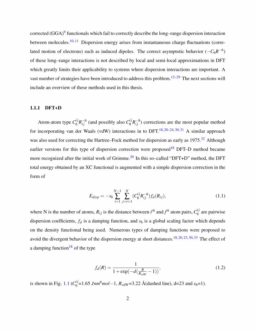
on the density functional being used. Numerous types of damping functions were proposed to
avoid the divergent behavior of the dispersion energy at short distances.18, 20, 23, 30, 33 The effect of
a damping function18 of the type
fd(R) =1
1+ exp(−d( RRvdW−1))
, (1.2)
is shown in Fig. 1.1 (Ci j6 =1.65 Jnm6mol−1, RvdW =3.22 A(dashed line), d=23 and s6=1).
2
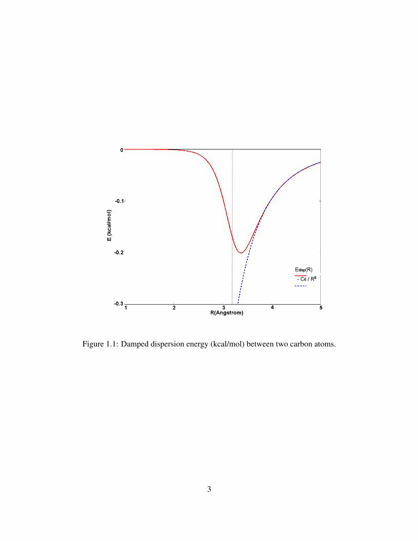
Figure 1.1: Damped dispersion energy (kcal/mol) between two carbon atoms.
3
The dispersion energy correction term is calculated separately from the DFT calculation. Since
it is a long-range effect its influence on the electron densities should be small which allows a
separate calculation for the correction. This method is general and can be combined with any
exchange-correlation functional, with C6 coefficients being determined either empirically18, 20 or
ab-initio methods.22–24 Obtaining an accurate set of coefficients is of vital importance. Next, I will
summarize the methods used in this thesis for dispersion correction namely, DFT–D2, DFT–D3,
vdW–TS, vdW–DF and RPA.
In an earlier version of the DFT–D method Wu et al18 calculated empirical atomic Ci j6 coef-
ficients for by least squares fitting from experimental molecular Ci j6 coefficients obtained by using
dipole oscillator strength distributions (DOSD’s). Grimme20 initially used the Ci j6 coefficients from
Wu et al18 while averaging them over possible hybridization states (for the carbon atom). Later, in
his less empirical DFT–D2 approach21 using DFT/PBE034 calculations of atomic ionization poten-
tials (Iip) and static dipole polarizabilities (α i) he computes the dispersion coefficient for an atom
with the equation:
Ci6 = 0.05NIi
pαi (1.3)
where N has values of 2,10,18,36 and 54 based on the atom’s position in the periodic table (Iip and
α i are in atomic units). Dispersion coefficients for elements up to Xe were made available but in
some cases like the group I and II metals averaged C6 coefficients from the preceding rare gas and
group III element were used. This caused problems such as Na and Mg atoms having the same
dispersion coefficients. A geometric mean combination rule of the form shown in Equation 1.4 is
used to get Ci j6 coefficients from atomic Ci
6 and C j6 coefficients.
Ci j6 =
√Ci
6C j6 (1.4)
Other than the above mentioned C6 averaging issue, two major shortcomings of the DFT–D2
approach are that the Ci j6 coefficients are invariant to chemical environment and the s6 scaling
factor, which is adjusted for each density functional, results in wrong asymptotic energies at long
range even if the C6 coefficients are correct.
4

Grimme and coworkers solved these limitations with the newer DFT–D3 approach.22 DFT-D3
method includes C6 and C8 terms for the 2 body dispersion correction and also an option for the 3
body dispersion correction.
Edisp = ∑AB
∑n=6,8
snCAB
nrn
ABfd,n(rAB) (1.5)
fd,n(rAB) =1
1+6(rAB(sr,nRAB0 ))−αn
(1.6)
The global scaling factor (sn), which depends on the density functional used, is only adjusted
for n > 6 (s6=1) to ensure the correct asymptotic behavior. This (s8 to be precise) is the first
parameter in DFT–D3 that is empirically determined for each different density functional. Along
with this change they have adopted the type of damping function (Eq. 1.6) initially used by Chai
and Head–Gordon33 which is more convenient for higher order dispersion correction. However, in
a more recent paper35 they have replaced this with the Becke–Johnson (BJ) type damping which
gives finite dispersion energies at shorter distances rather than ”zero” dispersion energy. They
have noted that although the BJ damping is the primary choice, overall this only provides a slightly
better (although more physically sound) energies for the tests they have performed.35 I have used
the damping function in Eq. 1.6 for the DFT–D3 calculations in this thesis. The sr,6 is the second
parameter (since sr,8 is set to be equal to 1) that is empirically determined by a least squares fit
to a big dataset of noncovalent interaction energies. The steepness parameters α6 and α8 were
manually set to be 14 and 16, respectively.
Dispersion coefficients are calculated via ab–initio time–dependent (TD) DFT, where C6s are
calculated using the Casimir–Polder equation (Eq. 1.7) with averaged dipole polarizabilities at
imaginary frequencies (α(iω)). α(iω) values were computed not for free atoms but using the
stable hydrides of each element (except the rare gas atoms).
CAB6 =
3π
∫∞
0α
A(iω)αB(iω)dω (1.7)
5
Grimme et al. propose to account for the chemical environment dependence of the dispersion
coefficients by using the number coordination number of the atoms. The idea is that bond for-
mation which induces a quenching in the atomic state that changed the excitation energies (hence
the polarizabilities) is responsible for the change in the dispersion coefficients. As the coordina-
tion number of an atom increases it can be thought of as being squeezed, hence the dispersion
coefficient decreases. The reference CAB6 coefficient calculated by the Casimir–Polder equation
is adjusted by using the coordination number for the atom pair in the system of interest. Higher
order C8 terms are then obtained using recursion relations using the C6 values. The accuracy of
the molecular C6 coefficients obtained theoretically can be tested using the experimentally known
dipole oscillator strength distributions (DOSDs). The DFT–D3 method gives an 8.4% mean abso-
lute error for the accuracy of the molecular C6 coefficients based on the DOSD data reported by
Meath et al.
Two other dispersion correction schemes (Becke–Jonhson and Tkatchenko–Sheffler)23, 24
that depend on the chemical environment of the atoms were proposed before DFT–D3. Around an
electron there is a depletion of density, which is named a exchange–correlation hole. The electron
and its exchange hole has zero charge overall but a non–zero dipole moment. The Becke–Johnson
model (which I have not used in my calculations for this theses, hence it will be summarized
briefly here) proposes the aspherical shape of this exchange-correlation hole which generates a
dipole moment as the source for the dispersion interaction. System dependent inter–atomic disper-
sion coefficients Ci j6 are obtained by using atomic polarizabilities and exchange(only)-hole dipole
moment using the equation 1.8. The dispersion coefficients respond to chemical environment in
two ways. One they are scaled using effective atomic volumes and secondly through the changes of
the exchange–hole which affect the dipole moments that appear in equation 1.8. The molecular C6s
obtained using this method give 12.2% mean absolute error (MAE) based on the data of Meath and
coworkers.22 One disadvantage of the BJ methods is that the computational cost is more expensive
(on the order of a hybrid DFT calculation) compared to other DFT–D methods.36
CAB6 =
αAαB〈d2x 〉A〈d2
x 〉B〈d2
x 〉AαB + 〈d2x 〉BαA
(1.8)
6
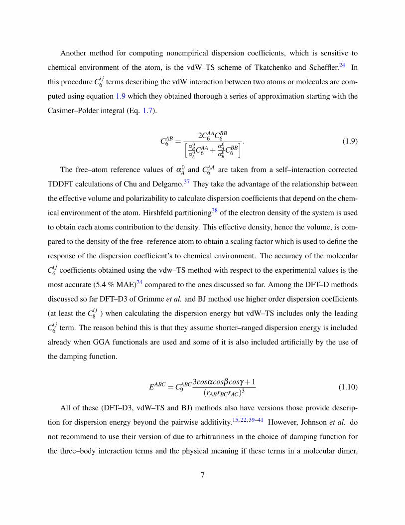
Another method for computing nonempirical dispersion coefficients, which is sensitive to
chemical environment of the atom, is the vdW–TS scheme of Tkatchenko and Scheffler.24 In
this procedure Ci j6 terms describing the vdW interaction between two atoms or molecules are com-
puted using equation 1.9 which they obtained thorough a series of approximation starting with the
Casimer–Polder integral (Eq. 1.7).
CAB6 =
2CAA6 CBB
6[α0
Bα0
ACAA
6 +α0
Aα0
BCBB
6
] . (1.9)
The free–atom reference values of α0A and CAA
6 are taken from a self–interaction corrected
TDDFT calculations of Chu and Delgarno.37 They take the advantage of the relationship between
the effective volume and polarizability to calculate dispersion coefficients that depend on the chem-
ical environment of the atom. Hirshfeld partitioning38 of the electron density of the system is used
to obtain each atoms contribution to the density. This effective density, hence the volume, is com-
pared to the density of the free–reference atom to obtain a scaling factor which is used to define the
response of the dispersion coefficient’s to chemical environment. The accuracy of the molecular
Ci j6 coefficients obtained using the vdw–TS method with respect to the experimental values is the
most accurate (5.4 % MAE)24 compared to the ones discussed so far. Among the DFT–D methods
discussed so far DFT–D3 of Grimme et al. and BJ method use higher order dispersion coefficients
(at least the Ci j8 ) when calculating the dispersion energy but vdW–TS includes only the leading
Ci j6 term. The reason behind this is that they assume shorter–ranged dispersion energy is included
already when GGA functionals are used and some of it is also included artificially by the use of
the damping function.
EABC =CABC9
3cosαcosβcosγ +1(rABrBCrAC)3 (1.10)
All of these (DFT–D3, vdW–TS and BJ) methods also have versions those provide descrip-
tion for dispersion energy beyond the pairwise additivity.15, 22, 39–41 However, Johnson et al. do
not recommend to use their version of due to arbitrariness in the choice of damping function for
the three–body interaction terms and the physical meaning if these terms in a molecular dimer,
7
and Grimme et al. decided to switch it off due to an overestimation of the three–body effects in
overlapping density regions with current density functionals and this leads to deterioration in the
performance of pairwise–additive only DFT–D3.22 For including the three–body terms Axilrod–
Teller–Muto equation (Eq. 1.10 ) has been used in all of the methods22, 39, 40 but the recent version
that was published by Tkatchenko and DiStasio.15, 41 This latest many–body dispersion method
(MBD) includes the long–range screening effects and many–body vdW energy to the all orders
of dipole interactions. In this method atoms are represented by quantum harmonic oscillators
(QHO) with characteristic frequency-dependent polarizabilities obtained with the aforementioned
vdW–TS method and the dispersion energy is obtained by solving the Schrodinger equation cor-
responding to these interacting QHOs within the dipole approximation. I will not go into more
detailed description of the many–body dispersion methods since they are not used in this thesis but
suffice it to say that these are found to be more important in modeling supramolecular systems42
and crystals.39, 43
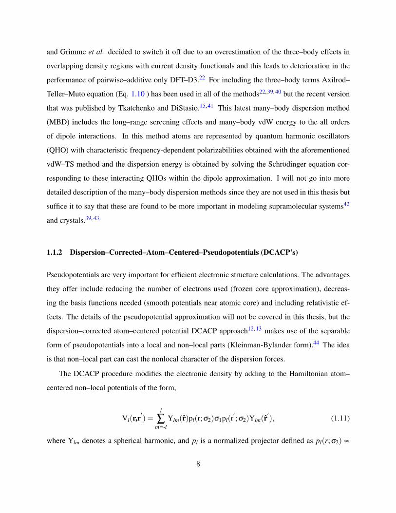
1.1.2 Dispersion–Corrected–Atom–Centered–Pseudopotentials (DCACP’s)
Pseudopotentials are very important for efficient electronic structure calculations. The advantages
they offer include reducing the number of electrons used (frozen core approximation), decreas-
ing the basis functions needed (smooth potentials near atomic core) and including relativistic ef-
fects. The details of the pseudopotential approximation will not be covered in this thesis, but the
dispersion–corrected atom–centered potential DCACP approach12, 13 makes use of the separable
form of pseudopotentials into a local and non–local parts (Kleinman-Bylander form).44 The idea
is that non–local part can cast the nonlocal character of the dispersion forces.
The DCACP procedure modifies the electronic density by adding to the Hamiltonian atom–
centered non–local potentials of the form,
Vl(r,r′) =
l
∑m=-l
Ylm(r)pl(r;σ2)σ1pl(r′;σ2)Ylm(r
′), (1.11)
where Ylm denotes a spherical harmonic, and pl is a normalized projector defined as pl(r;σ2) ∝
8

rlexp[–r2/2σ22 ] . The dispersion correction potentials are of the same functional form as the Gaus-
sian based non–local channels of the Goedecker–Teter–Hutter (GTH) pseudopotentials.45 The an-
alytical form of the GTH type pseudopotentials makes it easier to optimize the parameters needed
in DCACPs. The parameter σ1 scales the magnitude of the pseudopotential, and σ2 tunes the
location of the projector’s maximum from the atom center. In their application of this method,
Roethlisberger and coworkers used the l = 3 channel, and determined the σ1 and σ2 parameters
by use of a penalty function that minimized the differences between the DCACP and full CI or
CCSD(T)46 energies and forces evaluated at the equilibrium and midpoint geometries (the point
where the interaction energy equals half that of the equilibrium value – only for the energy term)
for a small set of dimers. This additional angular momentum dependent non–local part of the
pseudopotential does not interfere with the original pseudopotential since it acts further away from
the core region. The σ2 parameter that determines the location of the projector’s maximum for
the regular GTH atomic pseudopotentials is in the range of 0.2–0.3 A while in DCACP it varies
between 1.8–3.6 A. Also the σ1 which determines the magnitude is much smaller in the DCACP
potential compared to the regular GTH potential terms. The negligible difference in bond lengths
computed with the uncorrected density functional and its DCACP version gives additional support
that the new dispersion channel does not interfere with the atomic psedopotential.
The DCACP method has been implemented for the PBE,9 BLYP47, 48 and Becke-Perdew47, 49
functionals. It adds negligible computational cost to a DFT calculation. However, unlike DFT-
D methods, they permit a self-consistent treatment of electronic effects in a single DFT run and
no extra effort is needed to compute the forces on the ions. Currently these pseudopotentials are
available for a few elements of the periodic table.
Compared to the uncorrected GGA functionals the DCACP approach gives significantly im-
proved interaction energies for a wide range of systems near their equilibrium structures.12, 13, 50–55
However, the DCACP correction to the interaction energy falls off much more rapidly than R−6
with increasing distance between the monomers in a dimer.54–56 In Chapter 4, a study of isomers
of the water hexamer, we concluded that at least when used with the BLYP functional, DCACPs
are correcting for limitations of the functional in describing exchange-repulsion interaction as well
9
as for dispersion interactions.55
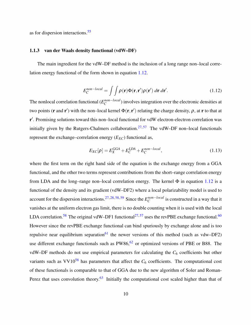
1.1.3 van der Waals density functional (vdW–DF)
The main ingredient for the vdW–DF method is the inclusion of a long range non–local corre-
lation energy functional of the form shown in equation 1.12.
Enon−localC =
∫ ∫ρ(r)Φ(r,r′)ρ(r′) dr dr′. (1.12)
The nonlocal correlation functional (Enon−localC ) involves integration over the electronic densities at
two points (r and r′) with the non–local kernel Φ(r,r′) relating the charge density, ρ , at r to that at
r′. Promising solutions toward this non–local functional for vdW electron-electron correlation was
initially given by the Rutgers-Chalmers collaboration.27, 57 The vdW–DF non–local functionals
represent the exchange–correlation energy (EXC) functional as,
EXC[ρ] = EGGAX +ELDA
C +Enon−localC , (1.13)
where the first term on the right hand side of the equation is the exchange energy from a GGA
functional, and the other two terms represent contributions from the short–range correlation energy
from LDA and the long–range non–local correlation energy. The kernel Φ in equation 1.12 is a
functional of the density and its gradient (vdW–DF2) where a local polarizability model is used to
account for the dispersion interactions.27, 28, 58, 59 Since the Enon−localC is constructed in a way that it
vanishes at the uniform electron gas limit, there is no double counting when it is used with the local
LDA correlation.58 The original vdW–DF1 functional27, 57 uses the revPBE exchange functional.60
However since the revPBE exchange functional can bind spuriously by exchange alone and is too
repulsive near equilibrium separation61 the newer versions of this method (such as vdw–DF2)
use different exchange functionals such as PW86,62 or optimized versions of PBE or B88. The
vdW–DF methods do not use empirical parameters for calculating the C6 coefficients but other
variants such as VV1058 has parameters that affect the C6 coefficients. The computational cost
of these functionals is comparable to that of GGA due to the new algorithm of Soler and Roman-
Perez that uses convolution theory.63 Initially the computational cost scaled higher than that of
10
GGAs and hybrid GGAs. Recent versions of this family of functionals provide very accurate C6
coefficients.25, 58, 64 Self–consistent versions of these methods are implemented in various codes.
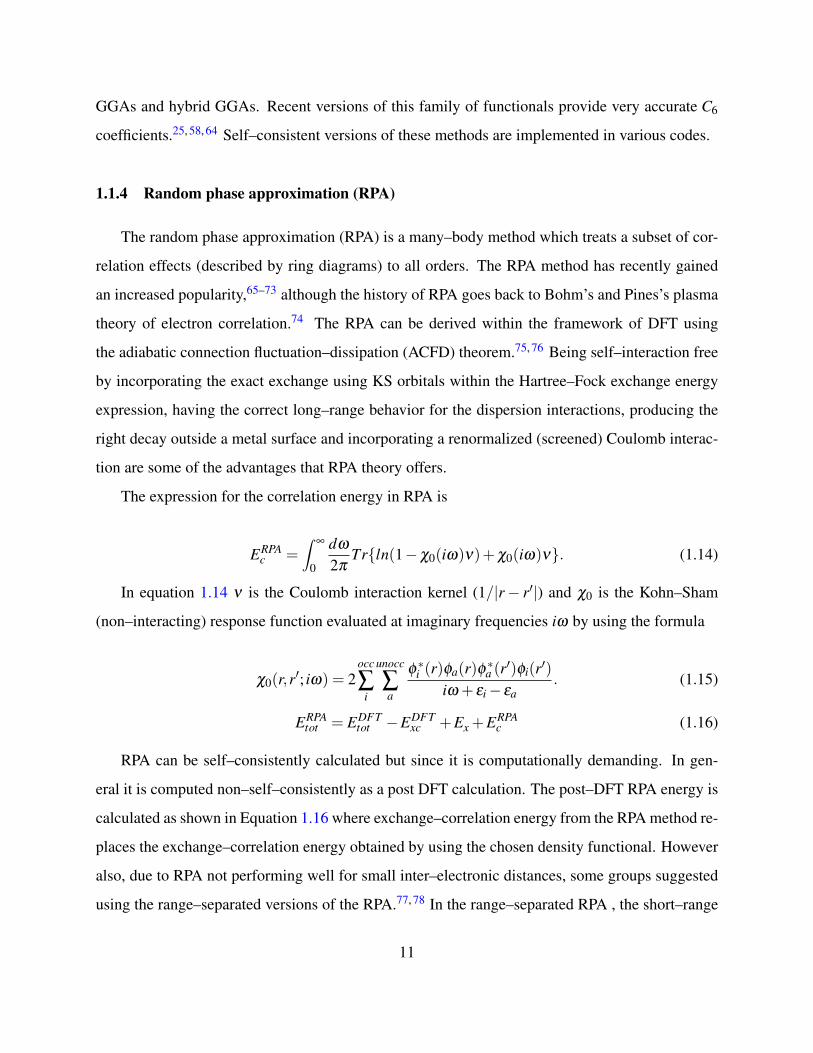
1.1.4 Random phase approximation (RPA)
The random phase approximation (RPA) is a many–body method which treats a subset of cor-
relation effects (described by ring diagrams) to all orders. The RPA method has recently gained
an increased popularity,65–73 although the history of RPA goes back to Bohm’s and Pines’s plasma
theory of electron correlation.74 The RPA can be derived within the framework of DFT using
the adiabatic connection fluctuation–dissipation (ACFD) theorem.75, 76 Being self–interaction free
by incorporating the exact exchange using KS orbitals within the Hartree–Fock exchange energy
expression, having the correct long–range behavior for the dispersion interactions, producing the
right decay outside a metal surface and incorporating a renormalized (screened) Coulomb interac-
tion are some of the advantages that RPA theory offers.
The expression for the correlation energy in RPA is
ERPAc =
∫∞
0
dω
2πTr{ln(1−χ0(iω)ν)+χ0(iω)ν}. (1.14)
In equation 1.14 ν is the Coulomb interaction kernel (1/|r− r′|) and χ0 is the Kohn–Sham
(non–interacting) response function evaluated at imaginary frequencies iω by using the formula
χ0(r,r′; iω) = 2occ
∑i
unocc
∑a
φ∗i (r)φa(r)φ∗a (r′)φi(r′)
iω + εi− εa. (1.15)
ERPAtot = EDFT
tot −EDFTxc +Ex +ERPA
c (1.16)
RPA can be self–consistently calculated but since it is computationally demanding. In gen-
eral it is computed non–self–consistently as a post DFT calculation. The post–DFT RPA energy is
calculated as shown in Equation 1.16 where exchange–correlation energy from the RPA method re-
places the exchange–correlation energy obtained by using the chosen density functional. However
also, due to RPA not performing well for small inter–electronic distances, some groups suggested
using the range–separated versions of the RPA.77, 78 In the range–separated RPA , the short–range
11

interactions are described via an exchange–correlation density functional while long–range ex-
change and correlation are treated by HF and RPA, respectively.
12
2.0 BENCHMARK CALCULATIONS OF WATER-ACENE INTERACTION
ENERGIES: EXTRAPOLATION TO THE WATER-GRAPHENE LIMIT AND
ASSESSMENT OF DISPERSION-CORRECTED DFT METHODS
This work was published as∗: Glen R. Jenness, Ozan Karalti, and Kenneth D. Jordan Physical
Chemistry Chemical Physics, 12, (2010), 6375–6381†
2.1 INTRODUCTION
In a previous study (J. Phys. Chem. C, 2009, 113, 10242–10248) we used density functional
theory based symmetry-adapted perturbation theory (DFT–SAPT) calculations of water interacting
with benzene (C6H6), coronene (C24H12), and circumcoronene (C54H18) to estimate the interac-
tion energy between a water molecule and a graphene sheet. The present study extends this earlier
work by use of a more realistic geometry with the water molecule oriented perpendicular to the
acene with both hydrogen atoms pointing down. We also include results for an intermediate C48H18
acene. Extrapolation of the water–acene results gives a value of −3.0± 0.15 kcal mol−1 for the
binding of a water molecule to graphene. Several popular dispersion-corrected DFT methods are
applied to the water–acene systems and the resulting interacting energies are compared to results
of the DFT–SAPT calculations in order to assess their performance.
The physisorption of atoms and molecules on surfaces is of fundamental importance in a
∗Reproduced by permission of the PCCP Owner Societies†G. R. J. contributed the majority of the numerical data. O. K. contributed the dispersion corrected DFT calcula-
tions.
13
wide range of processes. In recent years, there has been considerable interest in the interaction of
water with carbon nanotube and graphitic surfaces, in part motivated by the discovery that water
can fill carbon nanotubes.79 Computer simulations of these systems requires the availability of
accurate force fields and this, in turn, has generated considerable interest in the characterization of
the water–graphene potential using electronic structure methods.80–84
Density functional theory (DFT) has evolved into the method of choice for much theoretical
work on the adsorption of molecules on surfaces. However, due to the failure of the local density
approximation (LDA) and generalized gradient approximations (GGA) to account for long-range
correlation (hereafter referred to as dispersion or van der Waals) interactions, density functional
methods are expected to considerably underestimate the interaction energies for molecules on
graphitic surfaces. In recent years, several strategies have been introduced for “correcting” DFT
for dispersion interactions. These range from adding a pair-wise Cij6R−6
ij interactions,20, 21, 24, 64
to fitting parameters in functionals so that they better describe long-range dispersion,12, 13, 26, 56
to accounting explicitly for long-range non-locality, e.g., with the vdW–DF functional.27 Al-
though these approaches have been quite successful for describing dispersion interactions between
molecules, it remains to be seen whether they can accurately describe the interactions of water
and other molecules with carbon nanotubes or with graphene, given the tendency of DFT methods
to overestimate charge-transfer interactions85 and to overestimate polarization in extended conju-
gated systems.86 Thus, even if dispersion interactions were properly accounted for, it is not clear
how well DFT methods would perform at describing the interaction of polar molecules with ex-
tended acenes and graphene.
Second-order Moller–Plesset perturbation theory (MP2) does recover long-range two-body
dispersion interactions and has been used in calculating the interaction energies of water with
acenes as large as C96H24.80 However, MP2 calculations can appreciably overestimate two-body
dispersion energies.87, 88 This realization has led to the development of spin-scaled MP2 (SCS–
MP2),89, 90 empirically-corrected MP2,91 and “coupled” MP2 (MP2C)92 methods for better de-
scribing van der Waals interactions. However, it is not clear that even these variants of the MP2
method would give quantitatively accurate interaction energies for water or other molecules ad-
14

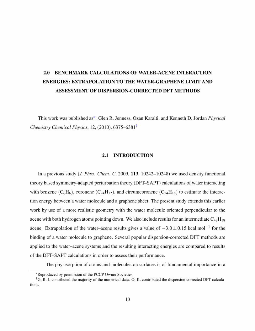
(a) Coronene (b) Hexabenzocoronene (HBC) (c) Dodecabenzocoronene (DBC)
Figure 2.1: Acenes used in the current study.
sorbed on large acenes since the HOMO–LUMO energy gap decreases with the size of the acene.
In addition to these issues, the MP2 method is inadequate for systems with large three-body dis-
persion contributions to the interaction energies.93
Given the issues and challenges described above, we have employed the DFT-based symmetry-
adapted perturbation theory (DFT–SAPT) method of Heßelmann et al.94 to calculate the inter-
action energies between a water molecule and benzene, coronene, hexabenzo[bc,ef,hi,kl,no,qr]-
coronene (referred to as hexabenzocoronene or HBC), and circumcoronene (also referred to as
dodecabenzocoronene or DBC). As will be discussed below, the DFT–SAPT approach has major
advantages over both traditional DFT and MP2 methods. The DFT–SAPT method also provides a
dissection of the net interaction energies into electrostatic, exchange-repulsion, induction, and dis-
persion contributions, which is valuable for the development of classical force fields and facilitates
the extrapolation of the results for the clusters to the water–graphene limit. In the current paper, we
extend our earlier study84 of water–acene systems to include more realistic geometrical structures.
The DFT–SAPT results are also used to assess various methods for including dispersion effects in
DFT calculations.
15
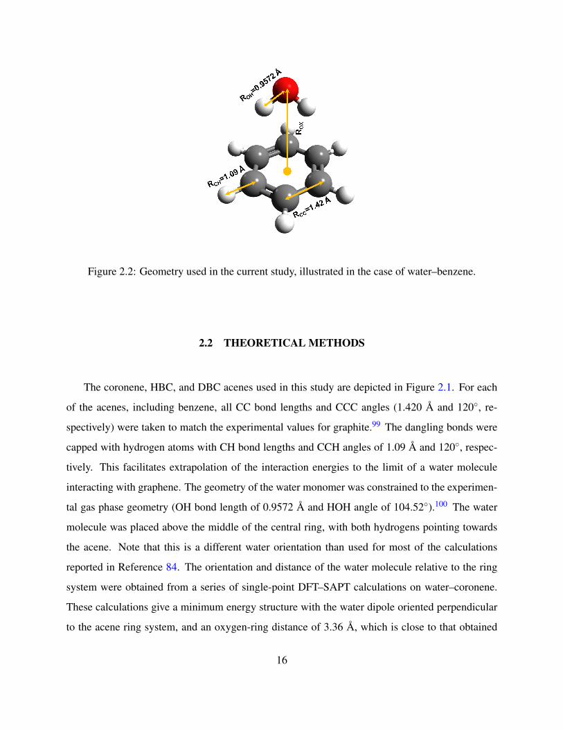
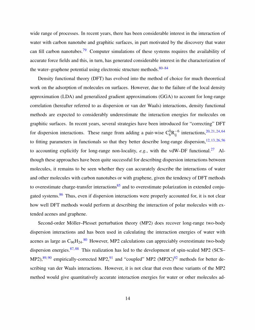
Figure 2.2: Geometry used in the current study, illustrated in the case of water–benzene.
2.2 THEORETICAL METHODS
The coronene, HBC, and DBC acenes used in this study are depicted in Figure 2.1. For each
of the acenes, including benzene, all CC bond lengths and CCC angles (1.420 A and 120◦, re-
spectively) were taken to match the experimental values for graphite.99 The dangling bonds were
capped with hydrogen atoms with CH bond lengths and CCH angles of 1.09 A and 120◦, respec-
tively. This facilitates extrapolation of the interaction energies to the limit of a water molecule
interacting with graphene. The geometry of the water monomer was constrained to the experimen-
tal gas phase geometry (OH bond length of 0.9572 A and HOH angle of 104.52◦).100 The water
molecule was placed above the middle of the central ring, with both hydrogens pointing towards
the acene. Note that this is a different water orientation than used for most of the calculations
reported in Reference 84. The orientation and distance of the water molecule relative to the ring
system were obtained from a series of single-point DFT–SAPT calculations on water–coronene.
These calculations give a minimum energy structure with the water dipole oriented perpendicular
to the acene ring system, and an oxygen-ring distance of 3.36 A, which is close to that obtained
16
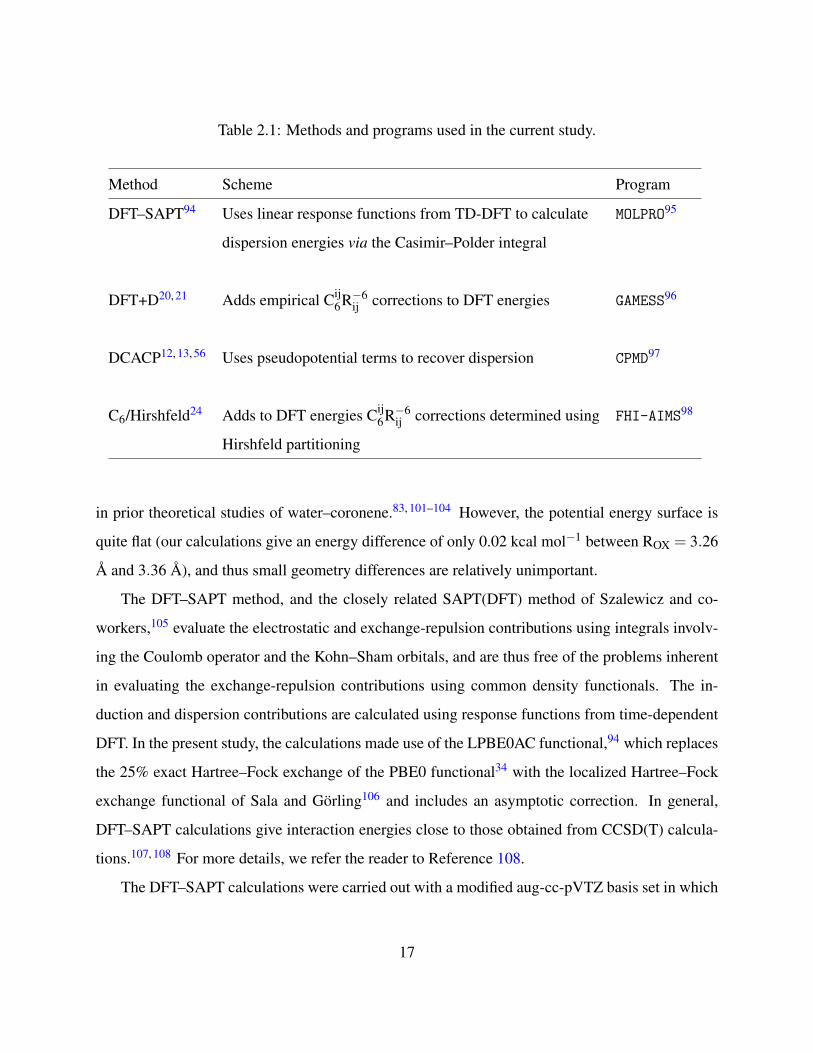
Table 2.1: Methods and programs used in the current study.
Method Scheme Program
DFT–SAPT94 Uses linear response functions from TD-DFT to calculate MOLPRO95
dispersion energies via the Casimir–Polder integral
DFT+D20, 21 Adds empirical Cij6R−6
ij corrections to DFT energies GAMESS96
DCACP12, 13, 56 Uses pseudopotential terms to recover dispersion CPMD97
C6/Hirshfeld24 Adds to DFT energies Cij6R−6
ij corrections determined using FHI-AIMS98
Hirshfeld partitioning
in prior theoretical studies of water–coronene.83, 101–104 However, the potential energy surface is
quite flat (our calculations give an energy difference of only 0.02 kcal mol−1 between ROX = 3.26
A and 3.36 A), and thus small geometry differences are relatively unimportant.
The DFT–SAPT method, and the closely related SAPT(DFT) method of Szalewicz and co-
workers,105 evaluate the electrostatic and exchange-repulsion contributions using integrals involv-
ing the Coulomb operator and the Kohn–Sham orbitals, and are thus free of the problems inherent
in evaluating the exchange-repulsion contributions using common density functionals. The in-
duction and dispersion contributions are calculated using response functions from time-dependent
DFT. In the present study, the calculations made use of the LPBE0AC functional,94 which replaces
the 25% exact Hartree–Fock exchange of the PBE0 functional34 with the localized Hartree–Fock
exchange functional of Sala and Gorling106 and includes an asymptotic correction. In general,
DFT–SAPT calculations give interaction energies close to those obtained from CCSD(T) calcula-
tions.107, 108 For more details, we refer the reader to Reference 108.
The DFT–SAPT calculations were carried out with a modified aug-cc-pVTZ basis set in which
17

the exponents of the diffuse functions were scaled by 2.0 to minimize convergence problems due
to near linear dependency in the basis set. In addition, for the carbon atoms the f functions were
removed and the three d functions were replaced with the two d functions from the aug-cc-pVDZ
basis set. Similarly, for the acene hydrogen atoms the d functions were removed and the three
p functions were replaced with the two p functions from the aug-cc-pVDZ basis set. The full
aug-cc-pVTZ basis set with the diffuse functions scaled by the same amount as the acene carbon
and hydrogen atoms was employed for the water molecule. For water–benzene, the DFT–SAPT
calculations with the modified basis set give an interaction energy only 0.05 kcal mol−1 smaller in
magnitude than that obtained with the full, unscaled, aug-cc-pVTZ basis set. Density fitting (DF)
using Weigend’s cc-pVQZ JK-fitting basis set109 was employed for the first order and the induction
and exchange-induction contributions. For the dispersion and exchange-dispersion contributions,
Weigend and co-worker’s aug-cc-pVTZ MP2-fitting basis set110 was used. The DF–DFT–SAPT
calculations were carried out with the MOLPRO ab initio package.95
We also examined several approaches for correcting density functional calculations for dis-
persion, including the dispersion-corrected atom-centered potential (DCACP) method of Roethlis-
berger,12, 13, 56 the DFT+dispersion (DFT+D) method of Grimme,20, 21 and the C6/Hirshfeld parti-
tioning scheme of Tkatchenko and Scheffler.24 The DCACP procedure uses modified Goedecker
pseudopotentials45 to incorporate dispersion effects. These calculations were carried out using the
CPMD program,97 utilizing a planewave basis set and periodic boundary conditions. These calcula-
tions employed a planewave cutoff of 4082 eV and box sizes of 42×42×28 a.u. for water–benzene
and water–coronene, and 46× 46× 28 a.u. for water–HBC and water–DBC to minimize interac-
tions between unit cells.
The DFT+D method adds damped empirical Cij6R−6
ij atom-atom corrections20, 21 to the “uncor-
rected” DFT energies. The DFT+D calculations were performed with the same Gaussian-type-
orbital basis sets as used in the DFT–SAPT calculations and were carried out using the GAMESS ab
initio package96 (using the implementation of Peverati and Baldridge111). The dispersion correc-
tions were added to the interaction energies calculated using the PBE,9 BLYP,47, 48 and B97–D21
GGA functionals. The B97-D functional is Grimme’s reparameterization of Becke’s B97 func-
18
tional112 for use with dispersion corrections.
The calculations involving the C6/Hirshfeld method of Tkatchenko and Scheffler24 were per-
formed with the FHI-AIMS package.98 The C6/Hirshfeld method, like the DFT+D method, in-
corporates dispersion via atom-atom Cij6R−6
ij terms. However, unlike the DFT+D method, the
C6/Hirshfeld scheme calculates the Cij6 coefficients using frequency-dependent polarizabilities for
the free atoms, scaling these values by ratios of the effective and free volumes, with the former
being obtained from Hirshfeld partitioning38 of the DFT charge density. This procedure results
in dispersion corrections that are sensitive to the chemical bonding environments. The tier 4 nu-
merical atom-centered basis sets113 native to FHI-AIMS were employed. These basis sets provide
a 6s5p4d3f 2g description of the carbon and oxygen atoms, and a 5s3p2d1f description of the
hydrogen atoms. A summary of the theoretical methods employed is given in Table 2.1.
2.3 RESULTS
2.3.1 DFT–SAPT calculations
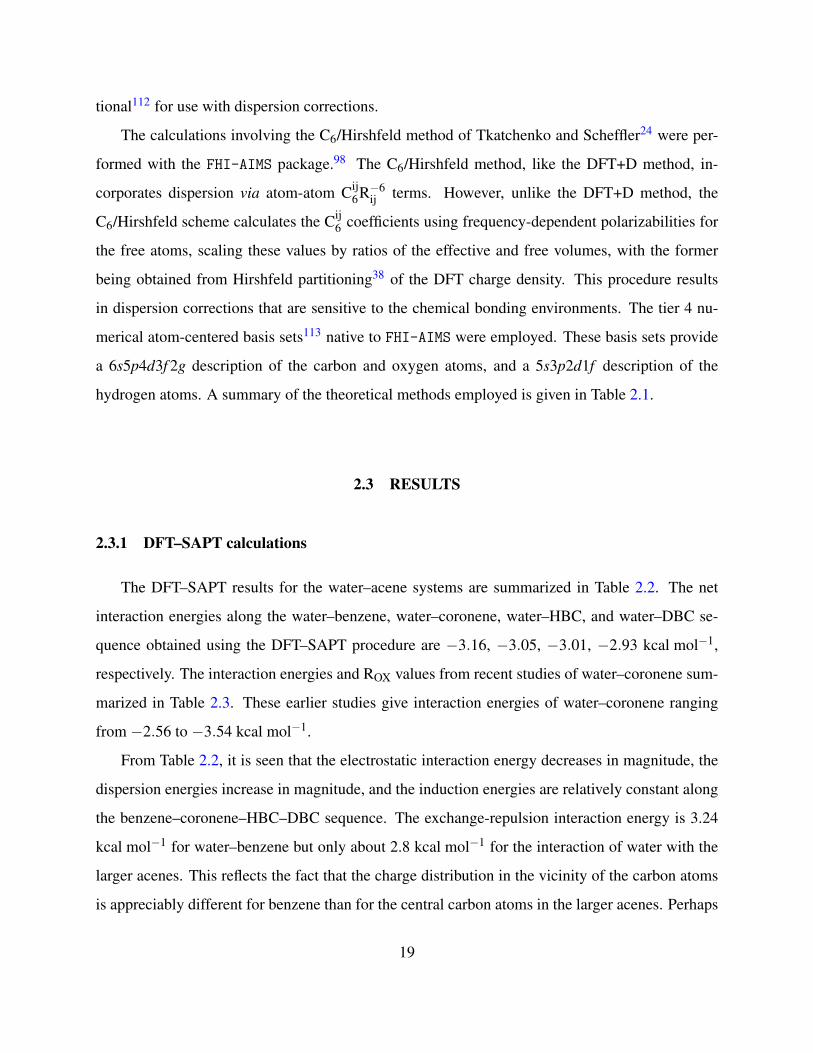
The DFT–SAPT results for the water–acene systems are summarized in Table 2.2. The net
interaction energies along the water–benzene, water–coronene, water–HBC, and water–DBC se-
quence obtained using the DFT–SAPT procedure are −3.16, −3.05, −3.01, −2.93 kcal mol−1,
respectively. The interaction energies and ROX values from recent studies of water–coronene sum-
marized in Table 2.3. These earlier studies give interaction energies of water–coronene ranging
from −2.56 to −3.54 kcal mol−1.
From Table 2.2, it is seen that the electrostatic interaction energy decreases in magnitude, the
dispersion energies increase in magnitude, and the induction energies are relatively constant along
the benzene–coronene–HBC–DBC sequence. The exchange-repulsion interaction energy is 3.24
kcal mol−1 for water–benzene but only about 2.8 kcal mol−1 for the interaction of water with the
larger acenes. This reflects the fact that the charge distribution in the vicinity of the carbon atoms
is appreciably different for benzene than for the central carbon atoms in the larger acenes. Perhaps
19

Table 2.2: Contributions to the DF–DFT–SAPT water–acene interaction energies (kcal mol−1).
Term Benzene Coronene HBC DBC
Electrostatics −2.85 −1.73 −1.54 −1.39
Exchange-repulsion 3.24 2.79 2.85 2.85
Induction −1.28 −1.29 −1.36 −1.37
Exchange-induction 0.82 0.80 0.83 0.84
δ (HF) −0.26 −0.20 −0.23 −0.23
Net induction −0.71 −0.69 −0.75 −0.75
Dispersion −3.28 −3.83 −4.00 (−4.07)a
Exchange-dispersion 0.44 0.42 0.43 (0.43)
Net dispersion −2.84 −3.42 −3.57 (−3.64)a
Total interaction energy −3.16 −3.05 −3.01 (−2.93)b
a Estimated using Edisp(water−DBC) = Edisp(water−HBC) +∑Cij6R−6
ij , where the Cij6R−6
ij terms account for the
dispersion interactions of the water molecule with the twelve additional C atoms of DBC. The C6 coefficients were
determined by fitting the DFT–SAPT water–coronene results.
b Total energy calculated using the estimated dispersion energy, described in footnote a.
20
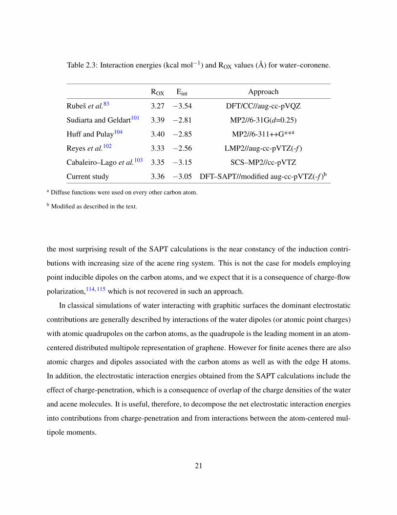
Table 2.3: Interaction energies (kcal mol−1) and ROX values (A) for water–coronene.
ROX Eint Approach
Rubes et al.83 3.27 −3.54 DFT/CC//aug-cc-pVQZ
Sudiarta and Geldart101 3.39 −2.81 MP2//6-31G(d=0.25)
Huff and Pulay104 3.40 −2.85 MP2//6-311++G**a
Reyes et al.102 3.33 −2.56 LMP2//aug-cc-pVTZ(-f )
Cabaleiro–Lago et al.103 3.35 −3.15 SCS–MP2//cc-pVTZ
Current study 3.36 −3.05 DFT–SAPT//modified aug-cc-pVTZ(-f )b
a Diffuse functions were used on every other carbon atom.
b Modified as described in the text.
the most surprising result of the SAPT calculations is the near constancy of the induction contri-
butions with increasing size of the acene ring system. This is not the case for models employing
point inducible dipoles on the carbon atoms, and we expect that it is a consequence of charge-flow
polarization,114, 115 which is not recovered in such an approach.
In classical simulations of water interacting with graphitic surfaces the dominant electrostatic
contributions are generally described by interactions of the water dipoles (or atomic point charges)
with atomic quadrupoles on the carbon atoms, as the quadrupole is the leading moment in an atom-
centered distributed multipole representation of graphene. However for finite acenes there are also
atomic charges and dipoles associated with the carbon atoms as well as with the edge H atoms.
In addition, the electrostatic interaction energies obtained from the SAPT calculations include the
effect of charge-penetration, which is a consequence of overlap of the charge densities of the water
and acene molecules. It is useful, therefore, to decompose the net electrostatic interaction energies
into contributions from charge-penetration and from interactions between the atom-centered mul-
tipole moments.
21
Tabl
e2.
4:M
ultip
ole
mom
ents
a(i
nat
omic
units
)for
the
carb
onan
dhy
drog
enat
oms
inbe
nzen
e,co
rone
ne,H
BC
and
DB
Cb .
Ato
mTy
peq
|µ|
Q20
|Q22
c+
Q22
s|
C6H
6C
24H
12C
42H
18C
54H
18C
6H6
C24
H12
C42
H18
C54
H18
C6H
6C
24H
12C
42H
18C
54H
18C
6H6
C24
H12
C42
H18
C54
H18
C1
−0.
09−
0.01
−0.
010.
000.
110.
010.
000.
00−
1.14
−1.
28−
1.29
−1.
280.
090.
000.
000.
00
C2
−0.
04−
0.01
0.00
0.11
0.02
0.01
−1.
22−
1.28
−1.
280.
090.
010.
01
C3
−0.
07−
0.03
−0.
010.
160.
080.
01−
1.17
−1.
25−
1.28
0.02
0.08
0.01
C4
−0.
08−
0.04
0.16
0.12
−1.
18−
1.22
0.04
0.10
C5
−0.
07−
0.07
0.13
0.16
−1.
13−
1.16
0.08
0.02
C5a
−0.
060.
16−
1.18
0.12
Hac
0.10
0.14
−0.
150.
09
Hbd
0.09
0.10
0.09
0.11
0.14
0.14
0.14
0.15
−0.
13−
0.13
−0.
13−
0.13
0.11
0.08
0.10
0.06
aSp
heri
cal
tens
orno
tatio
nis
empl
oyed
here
.To
conv
ert
into
aC
arte
sian
repr
esen
tatio
n:Θ
XX=−
1 2Q
20+
1 2
√3Q
22c;
ΘY
Y=−
1 2Q
20−
1 2
√3Q
22c;
ΘX
Y=−
1 2
√3Q
22s;
ΘZ
Z=
Q20
;
bB
enze
ne:C
6H6;
Cor
onen
e:C
24H
12;H
BC
:C42
H18
;DB
C:C
54H
18;
cH
ahy
drog
enat
oms
are
conn
ecte
dto
C4
carb
onat
oms.
dH
bhy
drog
enat
oms
are
conn
ecte
dto
C1
carb
ons
inbe
nzen
e,to
C3
carb
ons
inco
rone
ne,a
ndto
C5
carb
ons
inH
BC
and
DB
C.
22
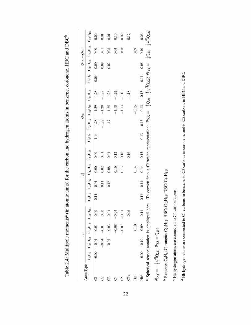
Table 2.5: Electrostatic energies (kcal mol−1) between atomic charges on water and multipoles.
Term Benzene Coronene HBC DBC Graphenea
Charge-Charge −1.36 −2.18 −1.89 −1.57 0.00
Charge-Dipole 1.86 3.20 2.53 2.01 0.00
Charge-Quadrupole −2.30 −2.13 −1.55 −1.22 −0.65b
Total multipole −1.80 −1.11 −0.91 −0.77 −0.65
Charge-penetration −1.05 −0.62 −0.62 −0.62 −0.62c
DFT–SAPT −2.85 −1.73 −1.54 −1.39 (−1.27)d
a Modeled by C216H36 as described in the text.
b Calculated by using atomic quadrupoles of Q20 =−1.28 a.u. on each carbon atom.
c The charge-penetration in the electrostatic interaction between water–graphene is assumed to be the same as between
water and DBC.
d Taken to be the sum of the charge-penetration (from water–DBC) and charge-quadrupole interactions for the water–
C216H36 model.
23
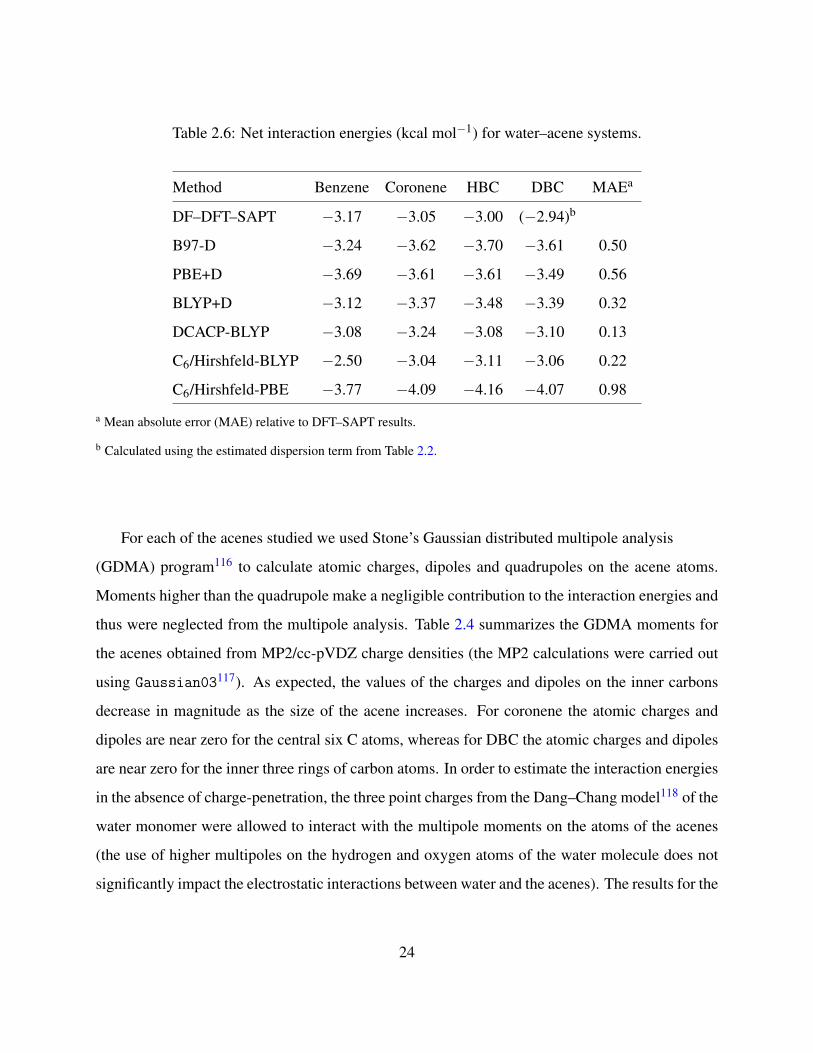
Table 2.6: Net interaction energies (kcal mol−1) for water–acene systems.
Method Benzene Coronene HBC DBC MAEa
DF–DFT–SAPT −3.17 −3.05 −3.00 (−2.94)b
B97-D −3.24 −3.62 −3.70 −3.61 0.50
PBE+D −3.69 −3.61 −3.61 −3.49 0.56
BLYP+D −3.12 −3.37 −3.48 −3.39 0.32
DCACP-BLYP −3.08 −3.24 −3.08 −3.10 0.13
C6/Hirshfeld-BLYP −2.50 −3.04 −3.11 −3.06 0.22
C6/Hirshfeld-PBE −3.77 −4.09 −4.16 −4.07 0.98
a Mean absolute error (MAE) relative to DFT–SAPT results.
b Calculated using the estimated dispersion term from Table 2.2.
For each of the acenes studied we used Stone’s Gaussian distributed multipole analysis
(GDMA) program116 to calculate atomic charges, dipoles and quadrupoles on the acene atoms.
Moments higher than the quadrupole make a negligible contribution to the interaction energies and
thus were neglected from the multipole analysis. Table 2.4 summarizes the GDMA moments for
the acenes obtained from MP2/cc-pVDZ charge densities (the MP2 calculations were carried out
using Gaussian03117). As expected, the values of the charges and dipoles on the inner carbons
decrease in magnitude as the size of the acene increases. For coronene the atomic charges and
dipoles are near zero for the central six C atoms, whereas for DBC the atomic charges and dipoles
are near zero for the inner three rings of carbon atoms. In order to estimate the interaction energies
in the absence of charge-penetration, the three point charges from the Dang–Chang model118 of the
water monomer were allowed to interact with the multipole moments on the atoms of the acenes
(the use of higher multipoles on the hydrogen and oxygen atoms of the water molecule does not
significantly impact the electrostatic interactions between water and the acenes). The results for the
24
various water–acene systems for ROX = 3.36 A are summarized in Table 2.5‡. The charge-charge,
charge-dipole and charge-quadrupole interactions are large in magnitude (≥1.2 kcal mol−1) for all
acenes considered, with the charge-charge and charge-quadrupole contributions being attractive
and the charge-dipole contributions being repulsive. Interestingly, the charge-dipole and charge-
quadrupole contributions roughly cancel for water–HBC and water–DBC. The charge-quadrupole
contribution decreases in magnitude with increasing size of the acene. This is a consequence of the
fact that the short-range electrostatic interactions with the carbon quadrupole moments are attrac-
tive while long-range interactions with the carbon quadrupoles are repulsive. The differences of
the SAPT and GDMA electrostatic energies provide estimates of the charge-penetration contribu-
tions which are found to be −0.62 kcal mol−1 for water–coronene, water–HBC, and water–DBC
for ROX = 3.36 A.
2.3.2 Dispersion-corrected DFT calculations
The interaction energies of the water–acene complexes (at ROX = 3.36 A) obtained using the
various dispersion-corrected DFT methods are reported in Table 2.6. Of the dispersion-corrected
DFT methods investigated, the DCACP method is the most successful at reproducing the DFT–
SAPT values of the interaction energies at ROX = 3.36 A. For water–coronene, water–HBC, and
water–DBC the interaction energies obtained with the C6/Hirshfeld method combined with the
BLYP functional are also in good agreement with the DFT–SAPT values, although this approach
underestimates the magnitude of the interaction energy for water–benzene by about 0.7 kcal mol−1.
Interestingly, with the exception of the PBE+D approach, all the dispersion-corrected DFT meth-
ods predict a larger in magnitude interaction energy for water–coronene than for water–benzene,
opposite from the results of the DFT–SAPT calculations. This could be due to the overestimation
of charge-transfer in the DFT methods, with the overestimation being greater for water–coronene.
Figure 2.3.2 reports the potential energy curves for the water–coronene and water–HBC systems
calculated with the various dispersion-corrected DFT methods. From Figures 3(a) and 3(b) it is
‡Due to a small conversion error, the actual electrostatic interactions for water-DBC in Table 2.5 differ from thosepublished in Reference 53. These values should be replaced with the following (in kcal mol−1): charge-charge=−1.44;charge-dipole=1.97; charge-quadrupole=−1.24; Total multipole=−0.71
25
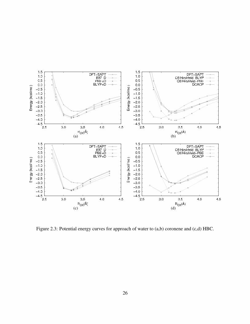
(a) (b)
(c) (d)
Figure 2.3: Potential energy curves for approach of water to (a,b) coronene and (c,d) HBC.
26

seen that the DFT+D methods and C6/Hirshfeld methods both tend to overbind the complexes.
The DFT+D methods with all three functionals considered and the C6/Hirshfeld calculations using
the BLYP functional locate the potential energy minimum at much smaller ROX values than found
in the DFT–SAPT calculations. It is also seen that the potential energy curves calculated using
the DCACP procedure differ significantly from the DFT–SAPT potential for ROX ≥ 4.2 A. This is
on account of the fact that the dispersion corrections in the DCACP method fall off much more
abruptly than R−6 at large R. It appears that part of the success of the DCACP method is actually
due to the pseudopotential terms improving the description of the exchange-repulsion contribution
to the interaction energies.
2.3.3 Extrapolation to the DFT–SAPT results to water–graphene
The exchange-repulsion, induction, exchange-dispersion, and charge-penetration contributions
between water and an acene are already well converged, with respect to the size of the acene,
by water–DBC. The contributions that have not converged by water–DBC are the non-charge-
penetration portion of the electrostatics and the dispersion (although the latter is nearly converged).
The non-charge-penetration contribution to the electrostatic energy for water–graphene was esti-
mated by calculating the electrostatic energy of water–C216H36 using only atomic quadrupoles on
the carbon atoms of the acene. The carbon quadrupole moments were taken to be Q20 =−1.28
a.u., the value calculated for the innermost six carbon atoms of DBC. We note that this value is
about twice as large in magnitude as that generally assumed for graphene.119 This gives an esti-
mate of −0.65 kcal mol−1 for the non-charge-penetration contribution to the electrostatic energy
between a water monomer and graphene.
Finally we estimate, using atomistic Cij6R−6
ij correction terms, that the dispersion energy is
about 0.05 kcal mol−1 larger in magnitude in water–graphene then for water–DBC. Adding the
various contributions we obtain a net interaction energy of −2.85 kcal mol−1 for water–graphene
assuming our standard geometry with ROX = 3.36 A. Rubes et al., extrapolating results obtained
using their DFT/CC method, predicted an interaction energy of −3.17 kcal mol−1 for water–
graphene. Interestingly, while Rubes et al. conclude the ROX is essentially the same for water–
27
coronene, water–DBC, and water–graphene, our DFT–SAPT calculations indicate that ROX in-
creases by about 0.15 A in going from water–coronene to water–HBC, with an energy lowering of
about 0.05 kcal mol−1 accompanying this increase of ROX for water–HBC. We further estimate,
based on calculations on water–benzene, that due to the basis set truncation errors, the DFT–SAPT
energies could be underestimated by as much as 0.1 kcal mol−1. Thus, we estimate that the “true”
interaction energy for water–graphene at the optimal geometry is −3.0±0.15 kcal mol−1, consis-
tent with the result of Rubes et al.83
2.4 CONCLUSIONS
In this study, we have used the DFT–SAPT procedure to provide benchmark results for the
interaction of a water molecule with a sequence of acenes up to C54H18 in size. All results
are for structures with the water molecule positioned above the central ring, with both hydro-
gen atoms down, and with the water–acene separation obtained from geometry optimization of
water–coronene. The magnitude of the interaction energy is found to fall off gradually along the
benzene–coronene–HBC–DBC sequence. This is on account of the fact that the electrostatic con-
tribution falls off more slowly with increasing ring size than the dispersion energy grows. We
combine the DFT–SAPT results with long-range electrostatic contributions calculated using dis-
tributed multipoles and long-range dispersion interactions calculated using Cij6R−6
ij terms to obtain
an estimate of the water–graphene interaction energy. This gives a net interaction energy of −2.85
kcal mol−1 for water–graphene assuming our standard geometry. We estimate that in the limit of
an infinite basis set and with geometry reoptimization, a value of −3.0± 0.15 kcal mol−1 would
result for the binding of a water molecule to a graphene sheet.
We also examined several procedures for correcting DFT calculations for dispersion. Of the
methods examined, the BLYP/DCACP approach gives interaction energies that are in the best
agreement with the results from the DFT–SAPT calculations. In an earlier work, it was shown that
the BLYP functional overestimates exchange-repulsion contributions,85 leading us to conclude that
28
the pseudopotential terms added in the DCACP procedure must also be correcting the exchange-
repulsion contributions.
Although the focus of this work has been on the interaction of a water molecule with a series
of acenes, the strategy employed is applicable for characterizing the interaction potentials of other
species with acenes and for extrapolating to the graphene limit. Although there is a large number
of theoretical papers addressing the interactions of various molecules with benzene, relatively lit-
tle work using accurate electronic structure methods has been carried out on molecules other than
water interacting with larger acenes.
2.5 ACKNOWLEDGEMENTS
This research was supported by the National Science Foundation (NSF) grant CHE-518253.
We would also like to thank Roberto Peverati for advice in using the DFT+D implementation in
GAMESS, Mike Schmidt for providing us with an advanced copy of the R4 release of GAMESS, and
to Wissam A. Al-Saidi for stimulating discussions.
29
3.0 EVALUATION OF THEORETICAL APPROACHES FOR DESCRIBING THE
INTERACTION OF WATER WITH LINEAR ACENES
This work was published as∗: Glen R. Jenness, Ozan Karalti, and Kenneth D. Jordan The
Journal of Physical Chemistry A, 115, (2011), 5955–5964†
3.1 INTRODUCTION
The interaction of a water monomer with a series of linear acenes (benzene, anthracene, pentacene,
heptacene, and nonacene) is investigated using a wide range of electronic structure methods, in-
cluding several “dispersion”-corrected density functional theory (DFT) methods, several variants
of the random phase approximation (RPA), DFT-based symmetry-adapted perturbation theory with
density fitting (DF–DFT–SAPT), MP2, and coupled-cluster methods. The DF–DFT–SAPT calcu-
lations are used to monitor the evolution of the electrostatics, exchange-repulsion, induction, and
dispersion contributions to the interaction energies with increasing acene size, and also provide the
benchmark data against which the other methods are assessed.
Graphene and graphite are prototypical hydrophobic systems.120 Interest in water inter-
acting with graphitic systems has also been motivated by the discovery that water can fill carbon
nanotubes.79 One of the challenges in modeling such systems is that experimental data for char-
acterizing classical force fields are lacking. Even the most basic quantity for testing force fields,
∗Reproduced by permission of the PCCP Owner Societies†O. K. contributed the dispersion corrected DFT and RPA calculations. G. R. J. contributed the calculations with
DFT–SAPT and wave–function methods.
30
the binding energy of a single water molecule to a graphene or graphite surface, is not known
experimentally. Several studies have appeared using electronic structure calculations to help fill
this void.53, 80–84, 101, 103, 104, 121–123 However, this is a very challenging problem since most DFT
methods rely on either local or semi–local density functionals that fail to appropriately describe
long-range dispersion interactions, which are the dominant attractive term in the interaction ener-
gies between a water molecule and graphene (or the acenes often used to model graphene).
In a recent study we applied the DF–DFT–SAPT procedure94 to a water molecule interact-
ing with a series of “circular” acenes (benzene, coronene, hexabenzo[bc,ef,hi,kl,no,qr]coronene,
and circumcoronene).53 These results were used to extrapolate to the binding energy of a water
molecule interacting with the graphene surface and also proved valuable as benchmarks for testing
other more approximate methods. Water–circumcoronene is essentially the limit of the size sys-
tem that can be currently be studied using the DF–DFT–SAPT method together with sufficiently
flexible basis sets to give nearly converged interaction energies. In the present study we consider a
water molecule interacting with a series of “linear” acenes, specifically, benzene, anthracene, pen-
tacene, heptacene, and nonacene, which allows us to explore longer-range interactions than in the
water–circumcoronene case and also explore in more detail the applicability of various theoretical
methods with decreasing HOMO/LUMO gap of the acenes. The theoretical methods considered
include DF–DFT–SAPT, several methods for correcting density functional theory for dispersion,
including the DFT–D2 and DFT–D3 schemes of Grimme and co-workers,21, 22 vdW–TS scheme
of Tkatchenko and Scheffler,24 the van der Waals density functional (vdW–DF) functionals of
Lundqvist, Langreth and co-workers,28, 124 and the dispersion-corrected atom-centered pseudopo-
tential (DCACP) method of Rothlisberger and co-workers.12, 56 Due to computational costs, only
a subset of these methods were applied to water–nonacene.
The results of these methods are compared to those from several wavefunction based methods,
including second-order Moller–Plesset perturbation theory (MP2),125 coupled-cluster with singles,
doubles and perturbative triples [CCSD(T)],46, 126, 127 spin-component-scaled MP2 (SCS–MP2),89
“coupled” MP2 (MP2C),92 and several variants of the random phase approximation (RPA).128–130
For comparative purposes, we also report interaction energies calculated using the recently intro-
31
duced DFT/CC method,83, 131 which combines DFT interaction energies with atom-atom correc-
tions based on coupled-cluster calculations on water–benzene.
3.2 THEORETICAL METHODS
The base DFT calculations for the DFT–D2 and DFT–D3 procedures and the CCSD(T), various
MP2, and DFT–SAPT calculations were performed with the MOLPRO95 ab initio package (version
2009.1). The DFT/CC corrections were calculated using a locally modified version of MOLPRO.
The dispersion corrections for the DFT–D2 and DFT–D3 procedures21, 22 were calculated using
the DFT-D3 program22 of Grimme and co-workers. The DCACP calculations were performed with
the CPMD97 code (version 3.11.1). The vdW–DF energies were computed non-self-consistently
using an in-house implementation of the Roman–Perez and Soler63 methodology and employing
densities from plane-wave DFT calculations carried out using the VASP code.132–135 The RPA and
vdW–TS calculations, including the base DFT (or Hartree–Fock) calculations required for both
methods, were carried out with the FHI-AIMS98 program (version 010110). The calculations with
MOLPRO used Gaussian-type orbital basis sets, those with FHI-AIMS employed numerical atom-
centered basis sets,113 and those with CPMD and VASP used plane-wave basis sets. Details about the
basis sets used are provided below.
3.2.1 Geometries
For the acenes, the same geometrical parameters were employed as in our earlier study of a
water molecule interacting with circular acenes,53 i.e., the CC and CH bond lengths were fixed at
1.42 A and 1.09 A, respectively, and the CCC and CCH bond angles were fixed at 120◦. Obviously,
the linear acenes in their equilibrium geometries have a range of CC bond lengths and CCC bond
angles; the fixed values given above were used as it facilitates comparison with our results for the
circular acenes. The experimental gas-phase geometry was used for the water monomer (OH bond
length of 0.9572 A and HOH angle of 104.52◦).100 The water monomer was positioned above the
32
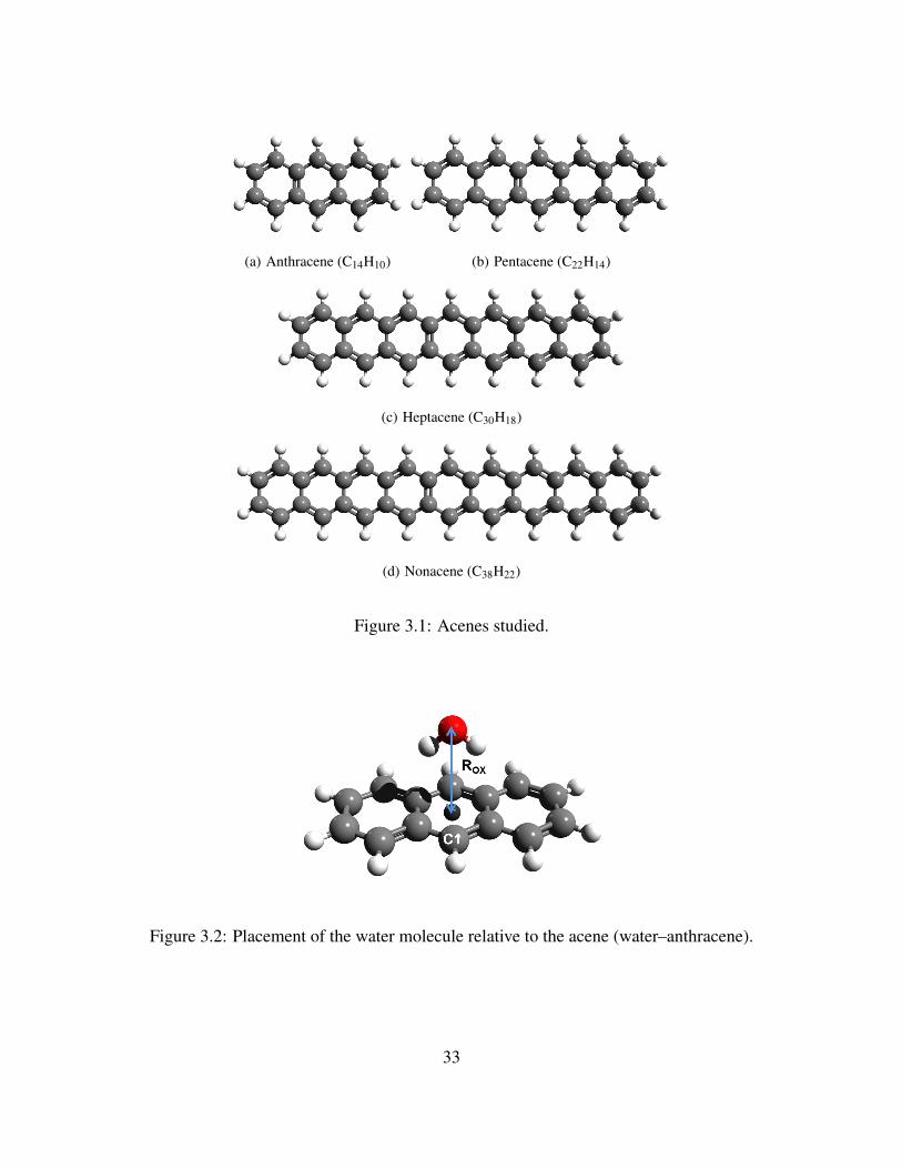
(a) Anthracene (C14H10) (b) Pentacene (C22H14)
(c) Heptacene (C30H18)
(d) Nonacene (C38H22)
Figure 3.1: Acenes studied.
Figure 3.2: Placement of the water molecule relative to the acene (water–anthracene).
33
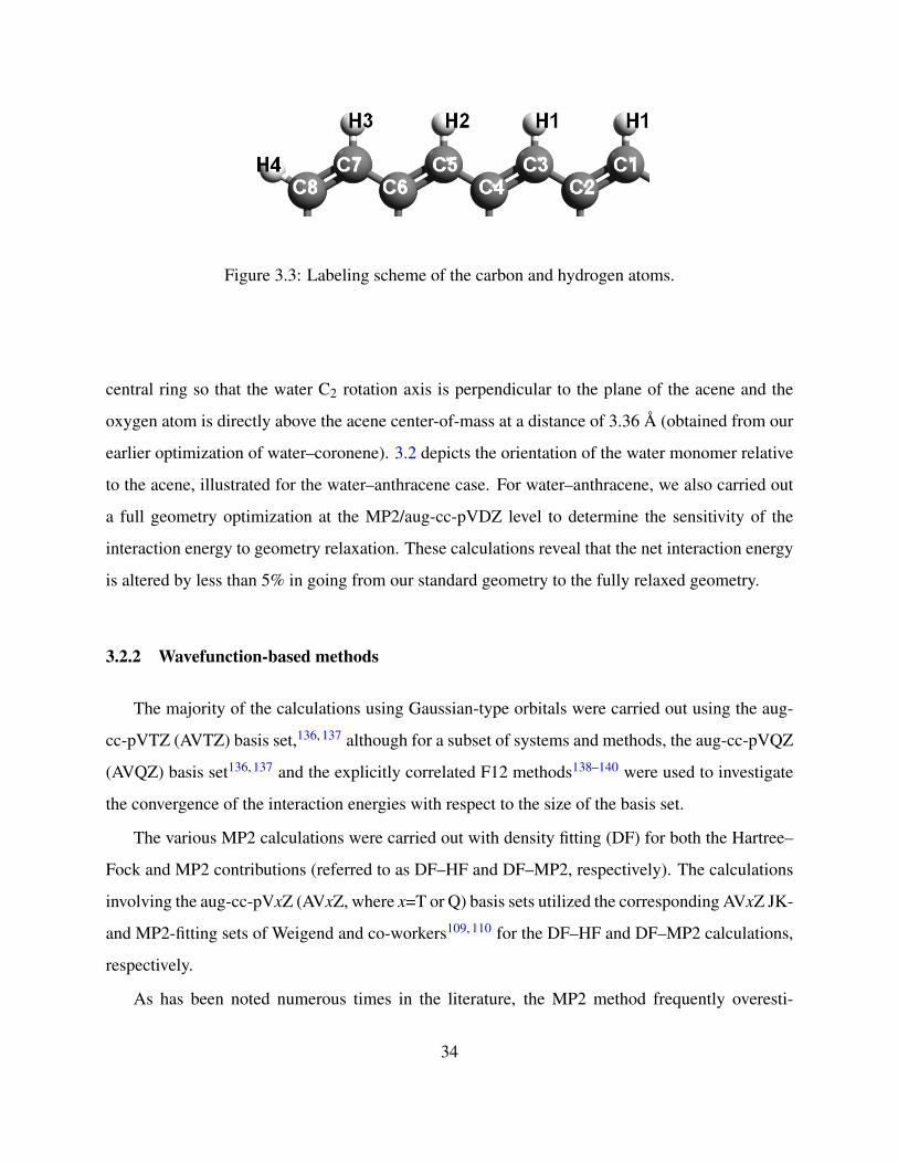
Figure 3.3: Labeling scheme of the carbon and hydrogen atoms.
central ring so that the water C2 rotation axis is perpendicular to the plane of the acene and the
oxygen atom is directly above the acene center-of-mass at a distance of 3.36 A (obtained from our
earlier optimization of water–coronene). 3.2 depicts the orientation of the water monomer relative
to the acene, illustrated for the water–anthracene case. For water–anthracene, we also carried out
a full geometry optimization at the MP2/aug-cc-pVDZ level to determine the sensitivity of the
interaction energy to geometry relaxation. These calculations reveal that the net interaction energy
is altered by less than 5% in going from our standard geometry to the fully relaxed geometry.
3.2.2 Wavefunction-based methods
The majority of the calculations using Gaussian-type orbitals were carried out using the aug-
cc-pVTZ (AVTZ) basis set,136, 137 although for a subset of systems and methods, the aug-cc-pVQZ
(AVQZ) basis set136, 137 and the explicitly correlated F12 methods138–140 were used to investigate
the convergence of the interaction energies with respect to the size of the basis set.
The various MP2 calculations were carried out with density fitting (DF) for both the Hartree–
Fock and MP2 contributions (referred to as DF–HF and DF–MP2, respectively). The calculations
involving the aug-cc-pVxZ (AVxZ, where x=T or Q) basis sets utilized the corresponding AVxZ JK-
and MP2-fitting sets of Weigend and co-workers109, 110 for the DF–HF and DF–MP2 calculations,
respectively.
As has been noted numerous times in the literature, the MP2 method frequently overesti-
34
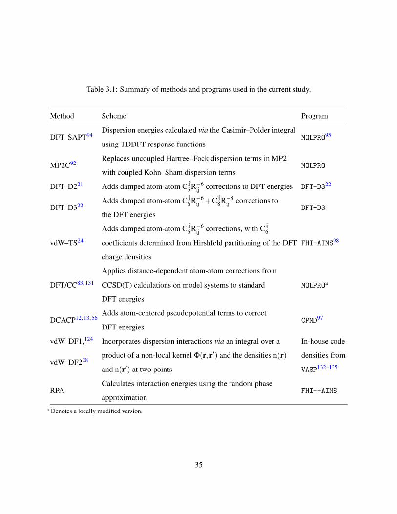
Table 3.1: Summary of methods and programs used in the current study.
Method Scheme Program
DFT–SAPT94Dispersion energies calculated via the Casimir–Polder integral
MOLPRO95
using TDDFT response functions
MP2C92Replaces uncoupled Hartree–Fock dispersion terms in MP2
MOLPROwith coupled Kohn–Sham dispersion terms
DFT–D221 Adds damped atom-atom Cij6R−6
ij corrections to DFT energies DFT-D322
DFT–D322Adds damped atom-atom Cij
6R−6ij +Cij
8R−8ij corrections to
DFT-D3the DFT energies
vdW–TS24
Adds damped atom-atom Cij6R−6
ij corrections, with Cij6
FHI-AIMS98coefficients determined from Hirshfeld partitioning of the DFT
charge densities
DFT/CC83, 131
Applies distance-dependent atom-atom corrections from
MOLPROaCCSD(T) calculations on model systems to standard
DFT energies
DCACP12, 13, 56Adds atom-centered pseudopotential terms to correct
CPMD97
DFT energies
vdW–DF1,124 Incorporates dispersion interactions via an integral over a In-house code
vdW–DF228product of a non-local kernel Φ(r,r′) and the densities n(r) densities from
and n(r′) at two points VASP132–135
RPACalculates interaction energies using the random phase
FHI--AIMSapproximation
a Denotes a locally modified version.
35
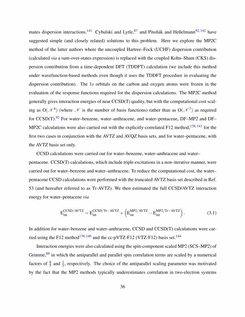
mates dispersion interactions.141 Cybulski and Lytle,87 and Pitonak and Heßelmann92, 142 have
suggested simple (and closely related) solutions to this problem. Here we explore the MP2C
method of the latter authors where the uncoupled Hartree–Fock (UCHF) dispersion contribution
(calculated via a sum-over-states expression) is replaced with the coupled Kohn–Sham (CKS) dis-
persion contribution from a time-dependent DFT (TDDFT) calculation (we include this method
under wavefunction-based methods even though it uses the TDDFT procedure in evaluating the
dispersion contribution). The 1s orbitals on the carbon and oxygen atoms were frozen in the
evaluation of the response functions required for the dispersion calculations. The MP2C method
generally gives interaction energies of near CCSD(T) quality, but with the computational cost scal-
ing as O(N 4) (where N is the number of basis functions) rather than as O(N 7) as required
for CCSD(T).92 For water–benzene, water–anthracene, and water–pentacene, DF–MP2 and DF–
MP2C calculations were also carried out with the explicitly-correlated F12 method,138, 143 for the
first two cases in conjunction with the AVTZ and AVQZ basis sets, and for water–pentacene, with
the AVTZ basis set only.
CCSD calculations were carried out for water–benzene, water–anthracene and water–
pentacene. CCSD(T) calculations, which include triple excitations in a non–iterative manner, were
carried out for water–benzene and water–anthracene. To reduce the computational cost, the water–
pentacene CCSD calculations were performed with the truncated AVTZ basis set described in Ref.
53 (and hereafter referred to as Tr-AVTZ). We then estimated the full CCSD/AVTZ interaction
energy for water–pentacene via
ECCSD/AVTZint = ECCSD/Tr−AVTZ
int +(
EMP2/AVTZint −EMP2/Tr−AVTZ
int
). (3.1)
In addition for water–benzene and water–anthracene, CCSD and CCSD(T) calculations were car-
ried using the F12 method139, 140 and the cc-pVTZ-F12 (VTZ-F12) basis set.144
Interaction energies were also calculated using the spin-component scaled MP2 (SCS–MP2) of
Grimme,89 in which the antiparallel and parallel spin correlation terms are scaled by a numerical
factors of 65 and 1
3 , respectively. The choice of the antiparallel scaling parameter was motivated
by the fact that the MP2 methods typically underestimates correlation in two-electron systems
36
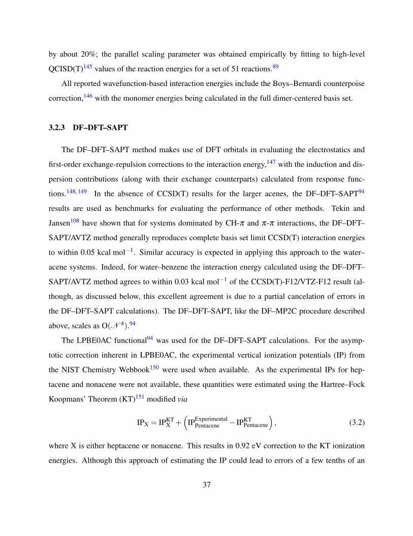
by about 20%; the parallel scaling parameter was obtained empirically by fitting to high-level
QCISD(T)145 values of the reaction energies for a set of 51 reactions.89
All reported wavefunction-based interaction energies include the Boys–Bernardi counterpoise
correction,146 with the monomer energies being calculated in the full dimer-centered basis set.
3.2.3 DF–DFT–SAPT
The DF–DFT–SAPT method makes use of DFT orbitals in evaluating the electrostatics and
first-order exchange-repulsion corrections to the interaction energy,147 with the induction and dis-
persion contributions (along with their exchange counterparts) calculated from response func-
tions.148, 149 In the absence of CCSD(T) results for the larger acenes, the DF–DFT–SAPT94
results are used as benchmarks for evaluating the performance of other methods. Tekin and
Jansen108 have shown that for systems dominated by CH-π and π-π interactions, the DF–DFT–
SAPT/AVTZ method generally reproduces complete basis set limit CCSD(T) interaction energies
to within 0.05 kcal mol−1. Similar accuracy is expected in applying this approach to the water–
acene systems. Indeed, for water–benzene the interaction energy calculated using the DF–DFT–
SAPT/AVTZ method agrees to within 0.03 kcal mol−1 of the CCSD(T)-F12/VTZ-F12 result (al-
though, as discussed below, this excellent agreement is due to a partial cancelation of errors in
the DF–DFT–SAPT calculations). The DF–DFT–SAPT, like the DF–MP2C procedure described
above, scales as O(N 4).94
The LPBE0AC functional94 was used for the DF–DFT–SAPT calculations. For the asymp-
totic correction inherent in LPBE0AC, the experimental vertical ionization potentials (IP) from
the NIST Chemistry Webbook150 were used when available. As the experimental IPs for hep-
tacene and nonacene were not available, these quantities were estimated using the Hartree–Fock
Koopmans’ Theorem (KT)151 modified via
IPX = IPKTX +
(IPExperimental
Pentacene − IPKTPentacene
), (3.2)
where X is either heptacene or nonacene. This results in 0.92 eV correction to the KT ionization
energies. Although this approach of estimating the IP could lead to errors of a few tenths of an
37

eV, these errors do not significantly impact the resulting water–acene interaction energies. For
example, a change of 0.1 eV in the IP of benzene results in a 0.01 kcal mol−1 change in the
interaction energy of water–benzene. For the density fitting, the cc-pV(x+1)Z JK-fitting set of
Weigend109 was employed for all non-dispersion terms, and the AVxZ MP2-fitting set of Weigend
and co-workers110 was used for the dispersion contributions.
We were unable to successfully complete the calculation of the dispersion energy of water–
nonacene using the DF–DFT–SAPT procedure. However the DF–MP2C procedure uses a closely
related scheme for evaluating the dispersion energy and gives the same dispersion contributions
for water–heptacene and water–nonacene, and moreover gives a dispersion contribution for water–
heptacene within 0.1 kcal mol−1 of the DF–DFT–SAPT result when used with the LPBE0AC
functional.
3.2.4 DFT-based methods
Among the dispersion-corrected DFT methods, the DFT–D2 scheme,21 which involves the
addition of damped atom-atom Cij6R−6
ij correction terms to the DFT intermolecular energies, is
the simplest scheme. A drawback to the DFT–D2 scheme is the lack of sensitivity of the Cij6
coefficients to the chemical environment. This is partially addressed in the DFT–D322 method
which introduces dispersion coefficients that depend on the coordination number of the atoms
involved and also includes damped Cij8R−8
ij contributions.22 In the present study, the DFT–D2 and
DFT–D3 schemes are used with the PBE,9 revPBE,60 and BLYP47, 48 density functionals together
with the AVTZ basis set. The resulting interaction energies are corrected for BSSE using the
counterpoise procedure.
The vdW–TS method24 also applies damped atom-atom Cij6R−6
ij corrections to DFT energies,
but it differs from DFT–D2 in that the Cij6 coefficients are adjusted using effective atomic vol-
umes obtained from Hirshfeld partitioning38 of the charge densities. The vdW–TS calculations
were performed with tier 3 and tier 4 numerical atom-centered basis sets113 for hydrogen and car-
bon/oxygen, respectively. These basis sets have been designed for use in FHI-AIMS. The tier 3
basis set provides a 5s3p2d1f description of the hydrogen atoms, and the tier 4 basis set provides
38
a 6s5p4d3f 2g description of the carbon/oxygen atoms. The largest vdW–TS calculation, that on
water–nonacene, employed 3864 basis functions.
The DFT/CC method of Rubes and co-workers83, 131 adds to the DFT energy atom-atom cor-
rection terms parameterized to differences between CCSD(T)/CBS and PBE interaction energies
for water–benzene. The DFT/CC method has been successfully used to categorize both solid152
and molecule–surface interactions.83, 121, 131 The reference energies used for the DFT/CC calcula-
tions were taken from Refs. 4 and 69. The base PBE energies for DFT/CC method were calculated
with the AVTZ basis set and were corrected for BSSE using the counterpoise procedure.
The dispersion-corrected atom-centered potential (DCACP) method of Roethlisberger and co-
workers12, 56 modifies Goedecker–Teter–Hutter (GTH) pseudopotentials45 by adding an f channel
to correct for deficiencies in the density functional employed. The calculations with the DCACPs
were carried out with a plane-wave basis set and using periodic boundary conditions. This ap-
proach was applied to acenes through heptacene and all calculations employed a planewave cutoff
of 3401 eV and a box size of 30×16×16 A. The high cut-off energy was necessitated by use of
the GTH pseudopotentials.
The vdW–DF1124 and vdW–DF228 GGA functionals of Langreth and coworkers represent the
exchange-correlation energy functional as
EXC[ρ] = EX +ELDAC +Enon−local
C , (3.3)
where the nonlocal correlation functional(Enonlocal
C)
involves integration over the electronic den-
sities (ρ) at two points (r and r′) with a non-local kernel (Φ(r,r′)),
Enon−localC =
12
∫ ∫ρ(r)Φ(r,r′)ρ(r′) dr dr′. (3.4)
As recommended by the developers, for vdW–DF1 and vdW–DF2, the revPBE and modified
PW8649 (called PW86R153) exchange density functionals were used, respectively. The vdW–DF
calculations were performed with charge densities from VASP132–135 calculations obtained using
VASP-native pseudopotentials together with a planewave cutoff of 800 eV and a supercell with
∼ 10 A of vacuum in all directions.
39
3.2.5 RPA-based methods
The random phase approximation (RPA) method is a many-body method which treats a subset
of correlation effects (described by ring diagrams) to all orders.154 There are multiple variants of
the RPA method, and in this work three different RPA schemes, denoted RPA, RPA+2OX, and
RPA/(HF+PBE), are considered. In each case the energy includes exact exchange contributions
computed using the Hartree–Fock expression using either the Hartree–Fock or Kohn–Sham or-
bitals. The RPA plus second-order exchange (RPA+2OX) approach128, 129 adds a second-order
exchange energy correction to the total RPA energy. In the RPA/(HF+PBE) scheme, suggested to
us by Ren and Blum,130 the RPA/PBE correlation correction is added to the Hartree–Fock energy.
For the RPA and RPA+2OX schemes the interaction energies obtained using orbitals from HF,
PBE, revPBE and BLYP calculations are reported. The RPA calculations were performed with a
modified tier 3 numerical atom-centered basis set with the highest angular momentum basis func-
tions from the full tier 3 basis set (i.e. the f functions from hydrogen, the g functions from oxygen,
and the f and g functions from carbon) being deleted. In addition, the core 1s orbitals were frozen.
3.3 RESULTS AND DISCUSSION
Before turning to the discussion on the interaction energies obtained using the various theo-
retical methods, it is instructional to examine the trends in the energy gaps between the highest
occupied molecular orbital (HOMO) and lowest unoccupied molecular orbital (LUMO) as a func-
tion of the length of the acene. The orbital energies have been calculated at the Hartree–Fock
level using the 6-31G* basis set.155, 156 This basis was chosen to avoid the low-lying unfilled or-
bitals corresponding to approximate continuum functions157 that would be present with a basis set
including diffuse functions. The resulting HOMO–LUMO gaps are 12.7, 7.9, 5.8, 4.7, and 4.1
eV along the sequence benzene, anthracene, pentacene, heptacene, and nonacene. This leads one
to anticipate growing multiconfigurational character in the wavefunctions with increasing length
of the acene. It has even been suggested that the linear acenes larger than pentacene have triplet
40

ground states,158 although more recent theoretical work indicates that they have singlet ground
states159 as assumed in our study. Ref. 159 also demonstrates the expected increase in the mul-
ticonfigurational character with increasing length of the acene, raising the possibility that some
theoretical methods may not properly describe the water–acene interaction energies for the larger
acenes.
3.3.1 DF–DFT–SAPT Results
From 3.2, which summarizes the results of the DF–DFT–SAPT calculations, it is seen that
the net interaction energy between the water molecule and the acene is nearly independent of the
size of the acene. The electrostatic and exchange-repulsion contributions both experience a sizable
reduction in magnitude in going from benzene to anthracene, with these changes being of oppo-
site sign and approximately compensating for one another. The exchange-repulsion contribution
is essentially constant from anthracene to nonacene, whereas the electrostatic interaction energy
continues to decrease in magnitude along the sequence of acenes, with the change in the electro-
static energy in going from water–heptacene to water–nonacene being only 0.03 kcal mol−1. The
induction energy, discussed in more detail below, is nearly constant across the series of acenes
while the dispersion energy grows in magnitude from water–benzene to water–heptacene, and be-
ing essentially the same for water–heptacene and water–nonacene. The fall off in the electrostatic
contribution is approximately compensated by the growing dispersion contribution with increasing
length of the acene.
For benzene, anthracene, pentacene, and heptacene, the atomic multipoles through hexade-
capoles were calculated using a distributed multipole analysis (DMA),116, 160–162 performed with
the GDMA116 program and using MP2/cc-pVDZ charge densities from Gaussian03117 calculations.
The resulting atomic multipoles (through the quadrupoles) are reported in the supporting infor-
mation (SI). The analysis was not done for nonacene as the atomic multipole moments for the
carbon atoms of the central ring are well converged by heptacene. The charges, dipole moments,
and quadrupole moments associated with the carbon atoms of the central ring undergo appre-
ciable changes in going from benzene to anthracene, but they are essentially unchanged along
41

Table 3.2: Contributions to the DF–DFT–SAPT interaction energies (kcal/mol).
Term Benzene Anthracene Pentacene Heptacene Nonacene
E(1)Elst −2.82 −2.29 −2.07 −2.01 −1.98
E(1)Exch 3.25 2.85 2.84 2.85 2.85
E(2)Ind −1.28 −1.22 −1.24 −1.26 −1.28
E(2)ExInd 0.83 0.76 0.76 0.77 0.77
δHF −0.26 −0.21 −0.21 −0.20 −0.21
Net Induction −0.71 −0.67 −0.69 −0.69 −0.72
E(2)Disp −3.38 −3.66 −3.72 −3.79 (−3.78) a
E(2)ExDisp 0.46 0.43 0.43 0.43 (0.43)b
Net Dispersion −2.92 −3.23 −3.29 −3.36 (−3.36)
DF–DFT–SAPT −3.20 −3.34 −3.21 −3.21 −3.21
a As discussed in 3.2.3, the DF–DFT–SAPT calculation of the dispersion energy of water–nonacene wasunsuccessful. The dispersion energy for water–nonacene was taken to be the same as that for water–heptacene asDF–MP2C calculations give the same dispersion energy for these two systems.b The exchange-dispersion energy of water–nonacene has been assumed to be the same as that for water–heptacene.
42
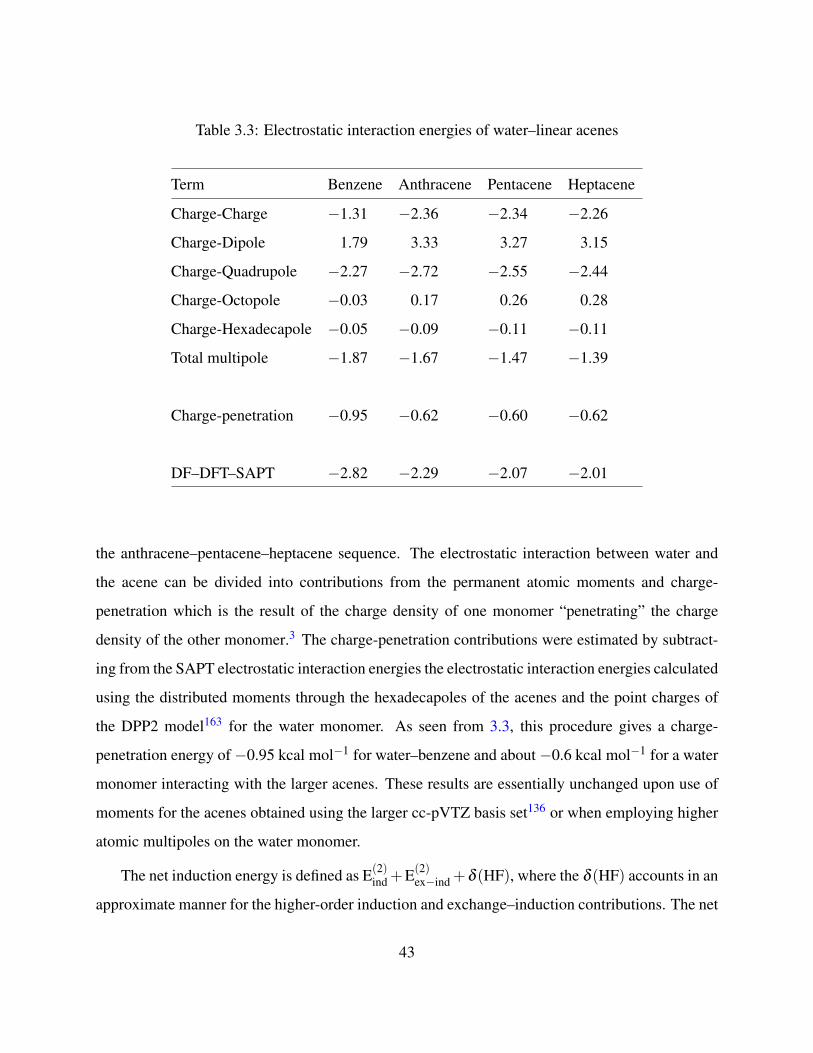
Table 3.3: Electrostatic interaction energies of water–linear acenes
Term Benzene Anthracene Pentacene Heptacene
Charge-Charge −1.31 −2.36 −2.34 −2.26
Charge-Dipole 1.79 3.33 3.27 3.15
Charge-Quadrupole −2.27 −2.72 −2.55 −2.44
Charge-Octopole −0.03 0.17 0.26 0.28
Charge-Hexadecapole −0.05 −0.09 −0.11 −0.11
Total multipole −1.87 −1.67 −1.47 −1.39
Charge-penetration −0.95 −0.62 −0.60 −0.62
DF–DFT–SAPT −2.82 −2.29 −2.07 −2.01
the anthracene–pentacene–heptacene sequence. The electrostatic interaction between water and
the acene can be divided into contributions from the permanent atomic moments and charge-
penetration which is the result of the charge density of one monomer “penetrating” the charge
density of the other monomer.3 The charge-penetration contributions were estimated by subtract-
ing from the SAPT electrostatic interaction energies the electrostatic interaction energies calculated
using the distributed moments through the hexadecapoles of the acenes and the point charges of
the DPP2 model163 for the water monomer. As seen from 3.3, this procedure gives a charge-
penetration energy of−0.95 kcal mol−1 for water–benzene and about−0.6 kcal mol−1 for a water
monomer interacting with the larger acenes. These results are essentially unchanged upon use of
moments for the acenes obtained using the larger cc-pVTZ basis set136 or when employing higher
atomic multipoles on the water monomer.
The net induction energy is defined as E(2)ind +E(2)
ex−ind +δ (HF), where the δ (HF) accounts in an
approximate manner for the higher-order induction and exchange–induction contributions. The net
43

(a)
(b)
(c)
Figure 3.4: Differences between Mulliken charges (me) in the presence and absence of the water.
44
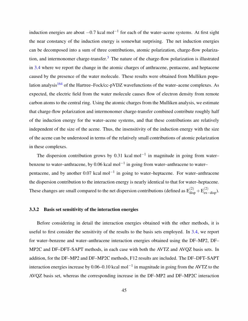
induction energies are about −0.7 kcal mol−1 for each of the water–acene systems. At first sight
the near constancy of the induction energy is somewhat surprising. The net induction energies
can be decomposed into a sum of three contributions, atomic polarization, charge-flow polariza-
tion, and intermonomer charge-transfer.3 The nature of the charge-flow polarization is illustrated
in 3.4 where we report the change in the atomic charges of anthracene, pentacene, and heptacene
caused by the presence of the water molecule. These results were obtained from Mulliken popu-
lation analysis164 of the Hartree–Fock/cc-pVDZ wavefunctions of the water–acene complexes. As
expected, the electric field from the water molecule causes flow of electron density from remote
carbon atoms to the central ring. Using the atomic charges from the Mulliken analysis, we estimate
that charge-flow polarization and intermonomer charge-transfer combined contribute roughly half
of the induction energy for the water–acene systems, and that these contributions are relatively
independent of the size of the acene. Thus, the insensitivity of the induction energy with the size
of the acene can be understood in terms of the relatively small contributions of atomic polarization
in these complexes.
The dispersion contribution grows by 0.31 kcal mol−1 in magnitude in going from water–
benzene to water–anthracene, by 0.06 kcal mol−1 in going from water–anthracene to water–
pentacene, and by another 0.07 kcal mol−1 in going to water–heptacene. For water–anthracene
the dispersion contribution to the interaction energy is nearly identical to that for water–heptacene.
These changes are small compared to the net dispersion contributions (defined as E(2)disp +E(2)
ex−disp).
3.3.2 Basis set sensitivity of the interaction energies
Before considering in detail the interaction energies obtained with the other methods, it is
useful to first consider the sensitivity of the results to the basis sets employed. In 3.4, we report
for water–benzene and water–anthracene interaction energies obtained using the DF–MP2, DF–
MP2C and DF–DFT–SAPT methods, in each case with both the AVTZ and AVQZ basis sets. In
addition, for the DF–MP2 and DF–MP2C methods, F12 results are included. The DF–DFT–SAPT
interaction energies increase by 0.06–0.10 kcal mol−1 in magnitude in going from the AVTZ to the
AVQZ basis set, whereas the corresponding increase in the DF–MP2 and DF–MP2C interaction
45
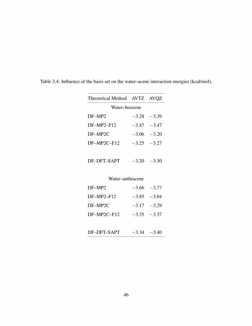
Table 3.4: Influence of the basis set on the water–acene interaction energies (kcal/mol).
Theoretical Method AVTZ AVQZ
Water–benzene
DF–MP2 −3.28 −3.39
DF–MP2–F12 −3.47 −3.47
DF–MP2C −3.06 −3.20
DF–MP2C–F12 −3.25 −3.27
DF–DFT–SAPT −3.20 −3.30
Water–anthracene
DF–MP2 −3.66 −3.77
DF–MP2–F12 −3.85 −3.84
DF–MP2C −3.17 −3.29
DF–MP2C–F12 −3.35 −3.37
DF–DFT–SAPT −3.34 −3.40
46

energies is 0.09–0.15 kcal mol−1. Moreover, with the latter two methods, the interaction energy
increases by another 0.05–0.08 kcal mol−1 in magnitude in going from the AVQZ basis set to the
F12/AVTZ procedure. The changes in the DF–MP2 and DF–MP2C interaction energies in going
from the F12/AVTZ to the F12/AVQZ approaches are 0.02 kcal mol−1 or less. These results justify
the use of the DF–DFT–SAPT/AVTZ approach to provide the benchmark results for assessing other
theoretical methods.
Thus for the MP2 and MP2C methods, the CBS-limit interaction energies are about 0.2
kcal mol−1 larger in magnitude than the results obtained using the AVTZ basis set. A similar
sensitivity to the basis set is found for the CCSD(T) interaction energy of water–benzene as seen
from 3.5. Moreover, the DF–MP2C and CCSD(T) procedures give nearly identical interaction
energies (we revisit the DF–MP2C interaction energies in the next section). It is also found that
the DF–DFT–SAPT calculations with the AVTZ basis set give interaction energies within a few
hundredths of a kcal mol−1 of the MP2C and CCSD(T) results obtained using the AVQZ/F12
method.
Although the interaction energies calculated with the DF–DFT–SAPT method are less sensitive
to the basis set than those calculated with the DF–MP2C or CCSD(T) methods, it is clear that in
the CBS-limit the DF–DFT–SAPT interaction energies would be about 0.1 kcal mol−1 larger in
magnitude than those obtained using the AVTZ basis set, resulting in slight overbinding of the
water–acene complexes.
3.3.3 Wavefunction-based results
Although the Hartree–Fock approximation predicts a monotonic fall off in the magnitude of the
interaction energy with increasing size of the acene, this is not the case for the DF–DFT–SAPT
method, the various DF–MP2 methods, or for the CCSD method. In each of these methods, the
interaction energy increases in magnitude in going from water–benzene to water–anthracene and
then drops off for the larger acenes. The origin of this behavior is clear from analysis of the results
in 3.2 and Table S1. Namely, the carbon atoms of benzene carry a greater negative charge than do
the carbon atoms of the central ring of the large acenes, causing the exchange-repulsion energy to
47
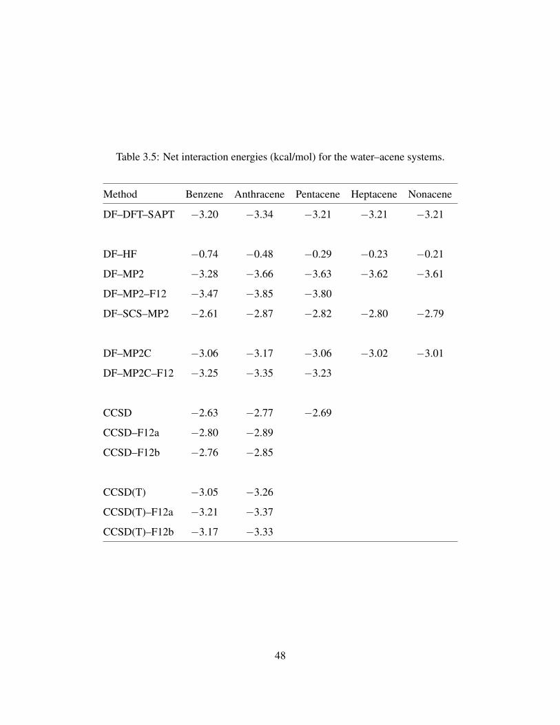
Table 3.5: Net interaction energies (kcal/mol) for the water–acene systems.
Method Benzene Anthracene Pentacene Heptacene Nonacene
DF–DFT–SAPT −3.20 −3.34 −3.21 −3.21 −3.21
DF–HF −0.74 −0.48 −0.29 −0.23 −0.21
DF–MP2 −3.28 −3.66 −3.63 −3.62 −3.61
DF–MP2–F12 −3.47 −3.85 −3.80
DF–SCS–MP2 −2.61 −2.87 −2.82 −2.80 −2.79
DF–MP2C −3.06 −3.17 −3.06 −3.02 −3.01
DF–MP2C–F12 −3.25 −3.35 −3.23
CCSD −2.63 −2.77 −2.69
CCSD–F12a −2.80 −2.89
CCSD–F12b −2.76 −2.85
CCSD(T) −3.05 −3.26
CCSD(T)–F12a −3.21 −3.37
CCSD(T)–F12b −3.17 −3.33
48
be greater in the case of water–benzene. This is the factor primarily responsible for the smaller in
magnitude interaction energy in water–benzene than in water–anthracene.
The interaction energies for the wavefunction based methods are presented in 3.5. For water–
benzene, water–anthracene, and water–pentacene the DF–MP2–F12 calculations overestimate the
binding energies by 0.27–0.59 kcal mol−1 in magnitude, with the discrepancy growing with in-
creasing size of the acene. On the other hand, the DF–SCS–MP2 method underestimates the mag-
nitude of the total interaction energies by 0.39 to 0.61 kcal mol−1. Comparison of the CCSD and
CCSD(T) results for water–benzene and water–anthracene shows that the inclusion of triple exci-
tations increases the interaction energies in magnitude by 0.4–0.5 kcal mol−1. Thus it appears that
the underestimation of the magnitude of the interaction energies with the DF–SCS–MP2 method
is due to the neglect of triple excitations.
The close agreement of the DF–MP2C, DF–DFT–SAPT and CCSD(T) interaction energies for
the water–acene systems warrants further discussion. A detailed analysis of wavefunction–based
SAPT [SAPT(HF)]165, 166 calculations on water–benzene reveals that intramonomer correlation a
−0.1 kcal mol−1 contribution to the dispersion portion of the interaction energy and a positive
contribution to both the exchange and electrostatic contributions to the interaction energy, with
the net change in the exchange plus electrostatics interaction being 0.65 kcal mol−1. On the other
hand, in the DF–MP2C approach there is a change of +0.2 kcal mol−1 in the dispersion energy
upon replacing the uncoupled Hartree–Fock dispersion contribution with the coupled Kohn–Sham
value.
Thus the good agreement between interaction energies obtained with the DF–MP2C method
and DF–DFT–SAPT approaches appears to be is due in part to a cancelation of errors in the former.
A closer examination of the SAPT(HF) results for intramonomer correlation on the dispersion
energy reveals that there are both large positive and negative corrections. It appears that although
the DF–MP2C method does not recover the 0.65 kcal mol−1 contribution of correlation effects to
the exchange and electrostatic energies, this is compensated by the failure to recover the −0.68
kcal mol−1 change in the dispersion energy due to intramonomer triple excitations.
49

3.3.4 DFT-based results
3.6 reports interaction energies obtained using the PBE, revPBE, and BLYP density functionals
with and without correcting for long-range dispersion. In considering these results, it should be
kept in mind that while GGA functionals do not capture long-range dispersion interactions, they
can describe short-range dispersion, and also that some dispersion-corrected DFT methods, such as
DCACP and DFT–D actually correct for deficiencies in DFT other than the absence of long-range
dispersion interactions.55
From 3.6 it can be seen that while the PBE functional recovers about half of the total interaction
energies for the water–acene systems, the revPBE and BLYP functionals predict binding only in the
water–benzene case. The failure to obtain bound complexes with the BLYP and revPBE functionals
is due to their larger (compared to PBE) exchange-repulsion contributions.85 Indeed this behavior
of the revPBE functional was the motivation for the switch from revPBE in vdW–DF1 to PW86 in
vdW–DF2.28
The DFT–D2 method does well at reproducing the DF–DFT–SAPT interaction energies with
mean absolute errors (MAEs) of 0.39, 0.15 and 0.02 kcal mol−1 for PBE, revPBE, and BLYP,
respectively. For all of the density functionals considered, the DFT–D3 approach overestimates
the magnitude of the interaction energies by about 0.5 kcal mol−1. This overestimation is partially
reduced if one uses the DFT–D3 parametrization based on the TZVPP167 basis set22 (denoted as
DFT–D3/TZ in 3.6).
The vdW–TS procedure based on the PBE functional overestimates the magnitude of the total
interaction energies, with a MAE of 0.67 kcal mol−1, while the vdW–TS procedure based on the
BLYP functional considerably underestimates the magnitude of the interaction energies. Given
the fact that the vdW–TS method employs dispersion corrections that depend on the chemical
environments, it is surprising that it performs poorer than DFT–D2 for the water–acene systems.
The DFT/CC method gives interaction energies very close to the DF–DFT–SAPT results (MAE
of 0.05 kcal mol−1). The DCACP/BLYP approach also gives interaction energies in excellent
agreement with the DF–DFT–SAPT results (MAE of 0.06 kcal mol−1) while the DCACP/PBE
approach, on the other hand, does not fair as well (MAE of 0.68 kcal mol−1). Both the vdW–DF1
50
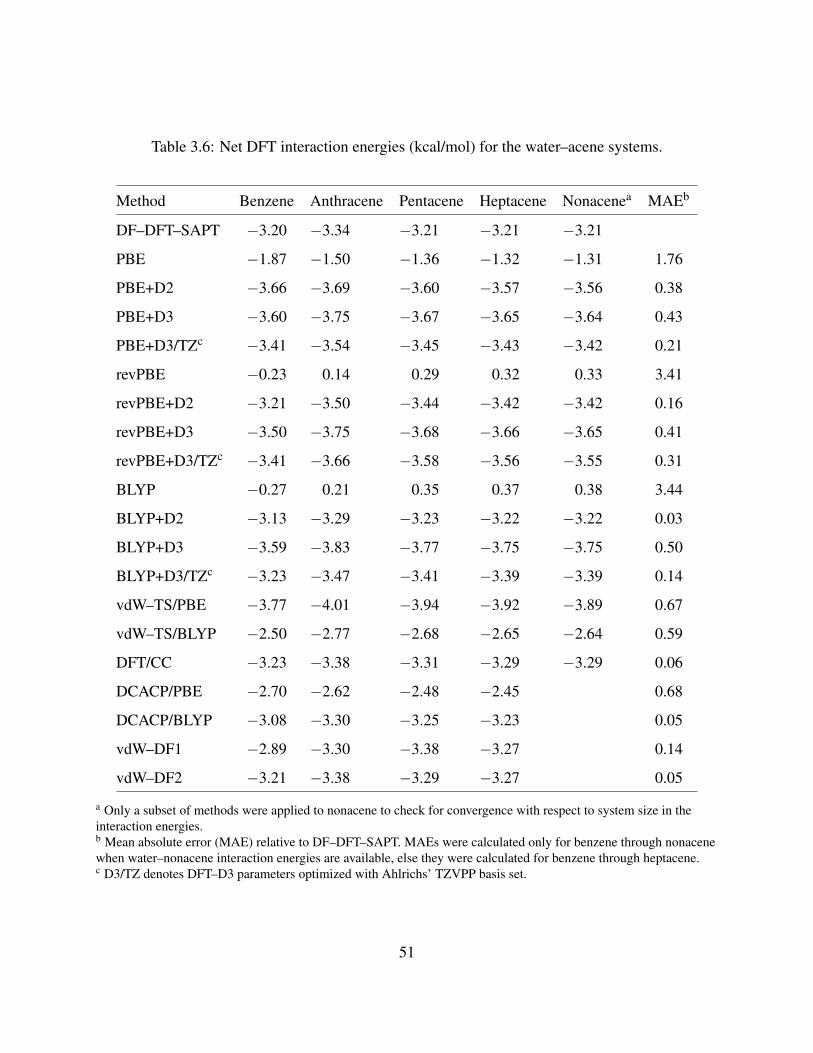
Table 3.6: Net DFT interaction energies (kcal/mol) for the water–acene systems.
Method Benzene Anthracene Pentacene Heptacene Nonacenea MAEb
DF–DFT–SAPT −3.20 −3.34 −3.21 −3.21 −3.21
PBE −1.87 −1.50 −1.36 −1.32 −1.31 1.76
PBE+D2 −3.66 −3.69 −3.60 −3.57 −3.56 0.38
PBE+D3 −3.60 −3.75 −3.67 −3.65 −3.64 0.43
PBE+D3/TZc −3.41 −3.54 −3.45 −3.43 −3.42 0.21
revPBE −0.23 0.14 0.29 0.32 0.33 3.41
revPBE+D2 −3.21 −3.50 −3.44 −3.42 −3.42 0.16
revPBE+D3 −3.50 −3.75 −3.68 −3.66 −3.65 0.41
revPBE+D3/TZc −3.41 −3.66 −3.58 −3.56 −3.55 0.31
BLYP −0.27 0.21 0.35 0.37 0.38 3.44
BLYP+D2 −3.13 −3.29 −3.23 −3.22 −3.22 0.03
BLYP+D3 −3.59 −3.83 −3.77 −3.75 −3.75 0.50
BLYP+D3/TZc −3.23 −3.47 −3.41 −3.39 −3.39 0.14
vdW–TS/PBE −3.77 −4.01 −3.94 −3.92 −3.89 0.67
vdW–TS/BLYP −2.50 −2.77 −2.68 −2.65 −2.64 0.59
DFT/CC −3.23 −3.38 −3.31 −3.29 −3.29 0.06
DCACP/PBE −2.70 −2.62 −2.48 −2.45 0.68
DCACP/BLYP −3.08 −3.30 −3.25 −3.23 0.05
vdW–DF1 −2.89 −3.30 −3.38 −3.27 0.14
vdW–DF2 −3.21 −3.38 −3.29 −3.27 0.05
a Only a subset of methods were applied to nonacene to check for convergence with respect to system size in theinteraction energies.b Mean absolute error (MAE) relative to DF–DFT–SAPT. MAEs were calculated only for benzene through nonacenewhen water–nonacene interaction energies are available, else they were calculated for benzene through heptacene.c D3/TZ denotes DFT–D3 parameters optimized with Ahlrichs’ TZVPP basis set.
51
and vdW–DF2 functionals give interaction energies close to the DF–DFT–SAPT values, with the
vdW–DF2 proving more successful at reproducing the trend in the interaction energies along the
sequence of acenes obtained from the DF–DFT–SAPT calculations.
3.3.5 RPA-based results
As seen from 3.7, the RPA calculations using HF orbitals give interaction energies about 0.9
kcal mol−1 smaller than the DF–DFT–SAPT results. The errors are reduced to about 0.6
kcal mol−1 when using RPA based on DFT orbitals for each of the three functionals considered.
The underestimation of the interaction energies is apparently a consequence of the limitations in the
RPA method at describing short-range correlation effects (which are not recovered by a sum over
ring diagrams only). Interestingly, Scuseria and co-workers have shown that the RPA method based
on Hartree–Fock orbitals corresponds to an approximate coupled-cluster doubles approximation.68
The present PBA/HF calculations on water-benzene, water-anthracene, and water-pentacene gives
binding energies 0.25–0.38 kcal mol−1 smaller in magnitude than the corresponding CCD results
(which, in turn, are nearly identical to the CCSD results in 3.5.
The RPA+2OX method does not correctly reproduce the trend in the interaction energies along
the sequence of acenes. It appears that the small HOMO/LUMO gaps in the DFT calculations on
the larger acenes result in nonphysical second-order exchange corrections. There is a significant
improvement in the interaction energies as calculated with the RPA/(HF+PBE) method, which
gives interaction energies 0.2–0.3 kcal mol−1 smaller in magnitude than the DF–DFT–SAPT re-
sults, which in turn are expected to be about 0.1 kcal mol−1 smaller in magnitude than the exact
interaction energies for the geometries employed. However, it is possible that the improved results
obtained with this approach are fortuitous as it obviously does not address the problem of RPA not
properly describing short-range correlation effects.
52

Table 3.7: Net RPA interaction energies (kcal/mol) for the water–acene systems.
Method Benzene Anthracene Pentacene Heptacene Nonacenea MAEb
DF–DFT–SAPT −3.20 −3.34 −3.21 −3.21 −3.21
RPA/HF −2.38 −2.42 −2.31 −2.27 −2.25 0.91
RPA/PBE −2.60 −2.70 −2.62 −2.59 0.61
RPA/revPBE −2.52 −2.69 −2.61 −2.59 0.64
RPA/BLYP −2.54 −2.73 −2.66 −2.63 0.60
RPA+2OX/HF −2.56 −2.53 −2.38 −2.37 0.78
RPA+2OX/PBE −3.18 −2.91 −2.66 −2.25 0.49
RPA+2OX/revPBE −3.15 −3.01 −2.76 0.28
RPA+2OX/BLYP −3.19 −3.03 −2.78 0.25
RPA/HF+PBE −2.90 −3.11 −3.05 −3.02 0.22
a Only a subset of methods were applied to nonacene to check for convergence with respect to system size in theinteraction energies.b Mean absolute error (MAE) relative to DF–DFT–SAPT. MAEs were calculated using results for benzene throughnonacene when water–nonacene interaction energies are available, else they were calculated for benzene throughheptacene.
53

Figure 3.5: Long-range interactions of water–benzene calculated with various methods.
3.3.6 Long-range interactions
All of the results discussed above have been for a water–acene complex with the water–acene
separation close to the potential energy minima (for the assumed orientation). 3.5 plots the long-
range interaction energies of various theoretical methods. For the DF–DFT–SAPT method the sum
of the dispersion and exchange-dispersion contributions is plotted, and for the DCACP/BLYP the
difference between the interaction energies with and without the DCACP correction is plotted. For
the DFT–D3/PBE method the dispersion contribution is plotted. For the vdW–DF1, vdW–DF2,
and RPA approaches, the differences of the correlation energies of the dimers and the correlation
energies of the monomers are plotted (using only the non-local correlation terms in the case of the
vdW–DF methods).
From 3.5, it is seen that the DFT–D3/PBE curve closely reproduces the DF–DFT–SAPT disper-
sion curve, indicating that this method is properly describing the dispersion energy in the asymp-
totic region. Both the vdW–DF2 and DCACP/BLYP methods give dispersion contributions that
54

fall off too rapidly for ROX ≥ 5.5 A (as noted in Ref. 58, the vdW–DF2 tends to underestimate
the C6 coefficients58). The vdW–DF1 curve, while being close to the SAPT curve for R & 8 A, is
much more attractive than the DF–DFT–SAPT curve for ROX ≤ 7.5 A.
The long-range interaction energy from the RPA/PBE calculations is repulsive from ROX = 5.5
to 10 A (the longest distance considered). This is due to the fact that the correlation correction in the
RPA method also describes the intramonomer correlation, which alters the electrostatic interaction
between the water monomer and the benzene molecule.
3.4 CONCLUSIONS
In the current study we examined the applicability of a large number of theoretical methods for
describing a water molecule interacting with a series of linear acenes. The DF–DFT–SAPT calcu-
lations, which provide the benchmark results against which the other methods are compared, give
interaction energies of water–benzene, water–anthracene, water–pentacene, and water–heptacene,
ranging from −3.20 to −3.24 kcal mol−1. This small spread in interaction energies is largely due
to the fact that the decreasing magnitude of the electrostatic interaction energy with increasing
size of the acene is partially compensated by the growing (in magnitude) dispersion contribution.
The DF–MP2C–F12/AVTZ approach, gives interaction energies in excellent agreement with the
DF–DFT–SAPT results, although this good agreement appears to be due, in part, to a cancelation
of errors in the DF–MP2C method.
Four of the DFT–corrected methods considered — BLYP–D2, DCACP/BLYP, DFT/CC and
vdW–DF2 — are found to give interaction energies for the water–acene systems very close to the
DF–DFT–SAPT results. The revPBE–D2, BLYP–D3/TZ, vdW–DF1, and PBE–D3/TZ approaches
also are reasonably successful at predicting the interaction energies at our standard geometries.
However these successes do not necessarily carry over to other geometries. In particular, as seen
in 3.5, both the DCACP and vdW–DF2 methods underestimate long-range dispersion interactions
in magnitude.
55

Even though the HOMO/LUMO gap decreases with increasing size of the acene, there is no
indication that any of the methods considered are encountering problems in the calculation of the
water–acene interaction energy even for acenes as large as nonacene.
3.5 ACKNOWLEDGEMENT
We would like to thank Professor A. Heßelmann for his advice concerning the use of the MP2C
method, Professor S. Grimme for providing us with a copy of his DFT-D3 program, and Professor
P. Nachtigall for discussions on DFT/CC. G. R. J. would like to personally thank the attendees
of the Telluride Many-Body Interactions 2010 Workshop for many insightful discussions. The
calculations were carried out on computer clusters in the University of Pittsburgh’s Center for
Molecular and Materials Simulations (CMMS).
56
4.0 IS THE DCACP METHOD PRIMARILY CORRECTING FOR DISPERSION?
4.1 INTRODUCTION
In the present study the performance of the dispersion–corrected atom–centered potential
(DCACP)12, 13 approach designed to add dispersion interaction missing in standard density func-
tional methods is analyzed for the low–energy ring, cage, prism, and book isomers of H2O)6. It
is concluded that for these clusters, the success of the DCACP method, particularly when used in
conjunction with BLYP functional, not only corrects for dispersion but also corrects for errors in
the non–dispersion contributions such as exchange to the interaction energies.
A major drawback of common GGA and hybrid density functional methods is the fail-
ure to describe long-range dispersion interactions which greatly limits their applicability to sys-
tems where such interactions are important. Not surprisingly, a large number of strategies have
been introduced to address this problem.12, 13, 18, 20–24, 26–29 These include adding Cij6R−6
ij (and
possibly also Cij8R−8
ij ) atom-atom type corrections,18, 20–24 fitting parameters in functionals26 or
additional pseudopotential terms,12, 13 to reproduce energies from accurate wavefunction calcula-
tions, and incorporating a non–local energy correction.27–29 In our work on water clusters85 and
on water interacting with acenes,53, 54 we have found that near the potential energy minima the
dispersion–corrected atom–centered potential (DCACP) procedure of Roethlisberger and cowork-
ers12, 13 gives interaction energies close to those obtained with symmetry-adapted perturbation
theory (SAPT).94, 105, 166 In the DCACP approach, standard pseudopotentials are augmented with
terms that are presumed to account for dispersion interactions missing in calculations using the
uncorrected functionals. In this note, we provide evidence that, when applied to water clusters and
57
used in conjunction with the BLYP functional,47, 48 the major effect of additional pseudopotential
terms is to correct for deficiencies in the exchange–repulsion interactions rather than to correct for
dispersion.
The DCACP procedure attempts to model long–range dispersion by adding terms to the
Hamiltonian of the form,
VDCACP(r,r’) = ∑m
Yl,mpl(r)σ1pl(r’)Y∗l,m, (4.1)
where Yl,m denotes a spherical harmonic, and projectors (pl) have the form
pl ∝ rl pl exp(−r2/2σ22 ), (4.2)
In their application of this method Roethlisberger and coworkers have taken l = 3, and have de-
termined the σ1 and σ2 parameters by use of a penalty functional that minimizes the differences
between the DCACP and full CI or CCSD(T) energies and forces at the equilibrium and midpoint
geometry (the point where the interaction energy equals half that of the equilibrium value). The
correction terms have the same analytical form as that used in the Goedecker–Teter–Hutter pseu-
dopotentials.45 The DCACP method has been implemented with PBE,9 BLYP47, 48 and Becke-
Perdew47, 49 functionals but most applications of the approach have been with the BLYP functional
,and we focus on this implementation in this article. We choose as our test systems, the ring, book,
cage and prism isomers of (H2O)6 (shown in Fig. 4.1) which have been the subject of numerous
studies.64, 85, 168–173
In a recent study,85 using both DFT and wavefunction-based methods, we decomposed the
net interaction energies of these isomers into their two-, three-, and four + five + six-body compo-
nents. We further separated the two- and three-body contributions from the DFT calculations into
electrostatics, exchange-repulsion, induction and intermonomer correlation contributions using the
LMO-EDA procedure,174 and compared these with analogous results from symmetry-adapted per-
turbation theory (SAPT).166 The inter-monomer correlation contributions from the DFT calcula-
tions were taken as approximately corresponding to the short-range part of the dispersion inter-
58
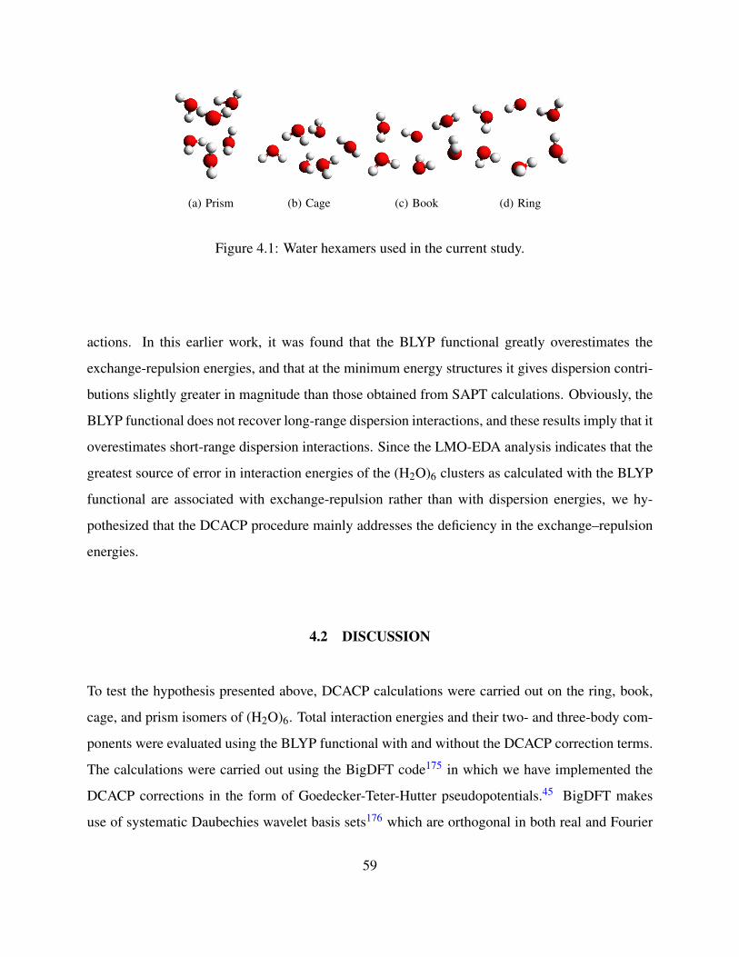
(a) Prism (b) Cage (c) Book (d) Ring
Figure 4.1: Water hexamers used in the current study.
actions. In this earlier work, it was found that the BLYP functional greatly overestimates the
exchange-repulsion energies, and that at the minimum energy structures it gives dispersion contri-
butions slightly greater in magnitude than those obtained from SAPT calculations. Obviously, the
BLYP functional does not recover long-range dispersion interactions, and these results imply that it
overestimates short-range dispersion interactions. Since the LMO-EDA analysis indicates that the
greatest source of error in interaction energies of the (H2O)6 clusters as calculated with the BLYP
functional are associated with exchange-repulsion rather than with dispersion energies, we hy-
pothesized that the DCACP procedure mainly addresses the deficiency in the exchange–repulsion
energies.
4.2 DISCUSSION
To test the hypothesis presented above, DCACP calculations were carried out on the ring, book,
cage, and prism isomers of (H2O)6. Total interaction energies and their two- and three-body com-
ponents were evaluated using the BLYP functional with and without the DCACP correction terms.
The calculations were carried out using the BigDFT code175 in which we have implemented the
DCACP corrections in the form of Goedecker-Teter-Hutter pseudopotentials.45 BigDFT makes
use of systematic Daubechies wavelet basis sets176 which are orthogonal in both real and Fourier
59
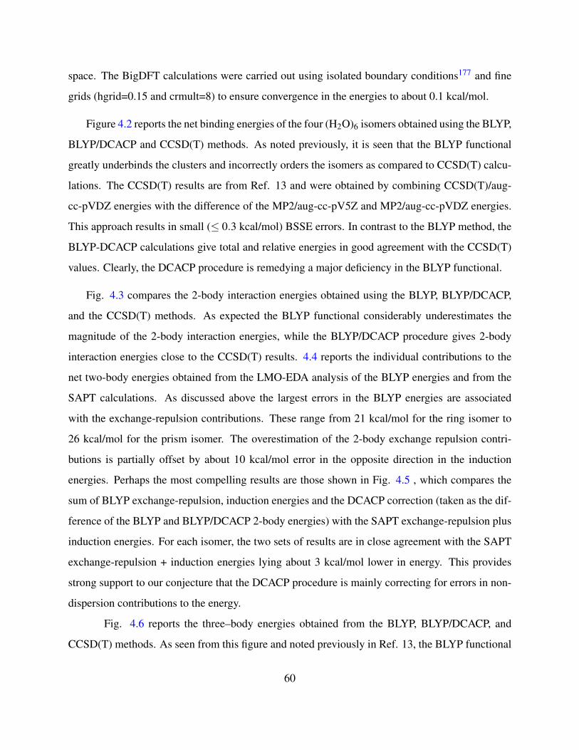
space. The BigDFT calculations were carried out using isolated boundary conditions177 and fine
grids (hgrid=0.15 and crmult=8) to ensure convergence in the energies to about 0.1 kcal/mol.
Figure 4.2 reports the net binding energies of the four (H2O)6 isomers obtained using the BLYP,
BLYP/DCACP and CCSD(T) methods. As noted previously, it is seen that the BLYP functional
greatly underbinds the clusters and incorrectly orders the isomers as compared to CCSD(T) calcu-
lations. The CCSD(T) results are from Ref. 13 and were obtained by combining CCSD(T)/aug-
cc-pVDZ energies with the difference of the MP2/aug-cc-pV5Z and MP2/aug-cc-pVDZ energies.
This approach results in small (≤ 0.3 kcal/mol) BSSE errors. In contrast to the BLYP method, the
BLYP-DCACP calculations give total and relative energies in good agreement with the CCSD(T)
values. Clearly, the DCACP procedure is remedying a major deficiency in the BLYP functional.
Fig. 4.3 compares the 2-body interaction energies obtained using the BLYP, BLYP/DCACP,
and the CCSD(T) methods. As expected the BLYP functional considerably underestimates the
magnitude of the 2-body interaction energies, while the BLYP/DCACP procedure gives 2-body
interaction energies close to the CCSD(T) results. 4.4 reports the individual contributions to the
net two-body energies obtained from the LMO-EDA analysis of the BLYP energies and from the
SAPT calculations. As discussed above the largest errors in the BLYP energies are associated
with the exchange-repulsion contributions. These range from 21 kcal/mol for the ring isomer to
26 kcal/mol for the prism isomer. The overestimation of the 2-body exchange repulsion contri-
butions is partially offset by about 10 kcal/mol error in the opposite direction in the induction
energies. Perhaps the most compelling results are those shown in Fig. 4.5 , which compares the
sum of BLYP exchange-repulsion, induction energies and the DCACP correction (taken as the dif-
ference of the BLYP and BLYP/DCACP 2-body energies) with the SAPT exchange-repulsion plus
induction energies. For each isomer, the two sets of results are in close agreement with the SAPT
exchange-repulsion + induction energies lying about 3 kcal/mol lower in energy. This provides
strong support to our conjecture that the DCACP procedure is mainly correcting for errors in non-
dispersion contributions to the energy.
Fig. 4.6 reports the three–body energies obtained from the BLYP, BLYP/DCACP, and
CCSD(T) methods. As seen from this figure and noted previously in Ref. 13, the BLYP functional
60

Figure 4.2: Net interaction energies of isomers of (H2O)6 (kcal/mol)
61
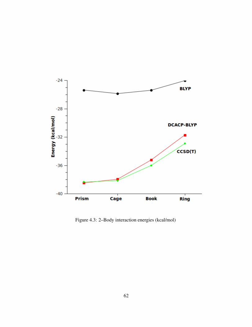
Figure 4.3: 2–Body interaction energies (kcal/mol)
62

Figure 4.4: Comparison of the individual contributions to the 2–body energy (kcal/mol)
63
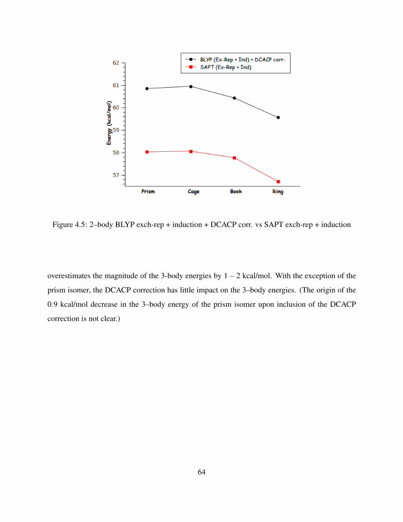
Figure 4.5: 2–body BLYP exch-rep + induction + DCACP corr. vs SAPT exch-rep + induction
overestimates the magnitude of the 3-body energies by 1− 2 kcal/mol. With the exception of the
prism isomer, the DCACP correction has little impact on the 3–body energies. (The origin of the
0.9 kcal/mol decrease in the 3–body energy of the prism isomer upon inclusion of the DCACP
correction is not clear.)
64
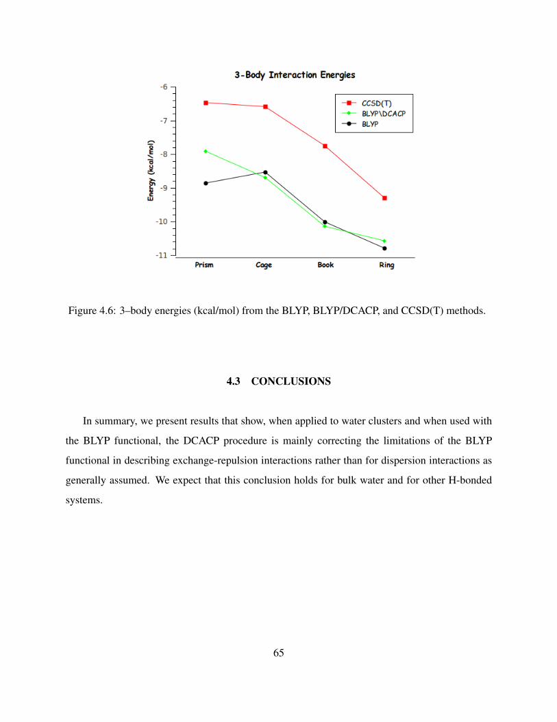
Figure 4.6: 3–body energies (kcal/mol) from the BLYP, BLYP/DCACP, and CCSD(T) methods.
4.3 CONCLUSIONS
In summary, we present results that show, when applied to water clusters and when used with
the BLYP functional, the DCACP procedure is mainly correcting the limitations of the BLYP
functional in describing exchange-repulsion interactions rather than for dispersion interactions as
generally assumed. We expect that this conclusion holds for bulk water and for other H-bonded
systems.
65
5.0 DCACP+D
5.1 INTRODUCTION
The dispersion–corrected atom–centered potential (DCACP)12, 13 approach, as discussed in the
previous three chapters, is a simple way of correcting density functional methods for dispersion
interactions. Although it provides very good accuracy for the interaction energies near equilibrium
distances, the energies fall off too quickly with the distance between the two moieties increases.
Also, as we have pointed in Chapter 4, at least, when used with the BLYP functional,47, 48 the
DCACP method is correcting for limitations of the functional in describing exchange-repulsion in-
teraction as well as for dispersion interactions. Actually, a similar effect is also noted for DFT+D
type dispersion corrections where the short–range damping function changes (corrects) the other
properties of the employed density functional.24 Here, we propose the ”DCACP+D” method
(which will be referred as DCACP/PBE-D3 or DCACP/BLYP-D3 throughout the text) for im-
proving the behavior of the long–range dispersion correction of the DCACPs. The main idea is to
use pseudopotentials to correct for the corresponding density functional’s deficiencies in describing
the interaction other than the dispersion and then for the dispersion energy to add on pairwise cor-
rections based on the Grimme (DFT–D3)22 and Tkatchenko-Sheffler (DFT+vdW–TS)24 schemes.
66

5.2 METHOD
The penalty functional used in this study differs from the Roethlisberger group’s version. In the cal-
ibration process of the pseudopotentials we try to reproduce the reference potential energy curves
by only using the energy terms (no force term is involved). As in the case of the original DCACP’s,
we use the l = 3 channel of the non–local part of the GTH pseudopotenial for the optimization.
We utilize the evolutionary algorithm coded in Dakota program for the minimization process.178
All DFT calculations were done with the CPMD program.97 Since the reference systems used
in the original DCACP show good transferability we decided to use the same set of dimers in
our fitting procedure. Parallel placed (H2)2, (N2)2, cross–shaped (CO2)2 and sandwich type ben-
zene dimer reference systems were used for the calibration of H, N, O and C pseudopotentials
respectively. The dispersionless potential energy curves of the reference dimers were calculated
by subtracting the DFT–SAPT94 dispersion energies from the CCSD(T) energies. DFT–SAPT
dispersion energies were calculated by adding the second–order dispersion energy and second–
order exhange–dispersion energy. In the case of (H2)2 aug-cc-pV5Z basis set136 was used for
the DFT–SAPT and CCSD(T) calculations. For the (N2)2 aug–cc–pVQZ basis set137 was used in
both type of calculations. In the (CO2)2 CCSD(T)–F12a method139 was used in conjunction with
the VTZ–F12144 basis set and DFT–SAPT calculations were done with aug-cc-pVQZ basis set.
For benzene dimer CCSD(T)/aug-cc-pVQZ quality binding energies were taken from a paper of
Sinnokrot et al.179 and DFT–SAPT calculations were done with aug-cc-pVQZ basis set. DFT–
D3//aug-cc-pVQZ calculations for the S22 set were obtained with Molpro, employing the initial
version damping function of the DFT–D3 method.22
In our first method proposal for improving the DCACPs, the dispersion correction part was
added on using the DFT–D3 method of Grimme.22 and the vdW–TS method of Tkatchenko et
al.24 In the version used in this work, vdW–TS method only adds damped C6/R6 terms onto the
DFT energy obtained using the fitted pseudopotentials while the Grimme version, in addition to the
damped C6/R6 term, also includes C8/R8 terms. We have used the BLYP47, 48 and PBE9 functionals
in our calculations. Since the energies obtained by the original density functionals were modified
67
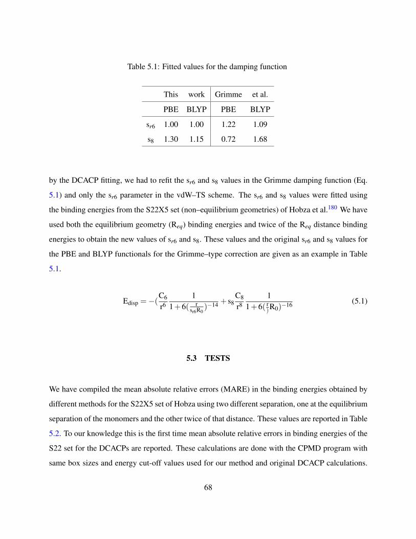
Table 5.1: Fitted values for the damping function
This work Grimme et al.
PBE BLYP PBE BLYP
sr6 1.00 1.00 1.22 1.09
s8 1.30 1.15 0.72 1.68
by the DCACP fitting, we had to refit the sr6 and s8 values in the Grimme damping function (Eq.
5.1) and only the sr6 parameter in the vdW–TS scheme. The sr6 and s8 values were fitted using
the binding energies from the S22X5 set (non–equilibrium geometries) of Hobza et al.180 We have
used both the equilibrium geometry (Req) binding energies and twice of the Req distance binding
energies to obtain the new values of sr6 and s8. These values and the original sr6 and s8 values for
the PBE and BLYP functionals for the Grimme–type correction are given as an example in Table
5.1.
Edisp =−(C6
r61
1+6( rsr6R0
)−14 + s8C8
r81
1+6( r)R0)−16 (5.1)
5.3 TESTS
We have compiled the mean absolute relative errors (MARE) in the binding energies obtained by
different methods for the S22X5 set of Hobza using two different separation, one at the equilibrium
separation of the monomers and the other twice of that distance. These values are reported in Table
5.2. To our knowledge this is the first time mean absolute relative errors in binding energies of the
S22 set for the DCACPs are reported. These calculations are done with the CPMD program with
same box sizes and energy cut-off values used for our method and original DCACP calculations.
68
Energies are well converged with respect to the cell dimensions and energy cut–off values.
The DCACP+D method based on the Grimme–type dispersion corrections for both of the den-
sity functionals (BLYP and PBE) shows improvement on the equilibrium binding energies of the
test set compared to the original DCACPs. Also in all cases a dramatic improvement is seen for
binding energies at 2Req. Although, the DCACP+D scheme augmented with the vdW–TS dis-
persion energies performs worse than the original DCACPs at Req, it reduces the error by half at
longer distance. The poor performance of the Tkatchenko–Sheffler method compared to Grimme’s
can be attributed to the neglect of the C8/R8 terms. In the vdW–TS scheme short–range correla-
tion (C8/R8 terms) is believed to be captured by the semi–local DFT functionals. However, due to
the dispersionless fitting procedure we use, the functionals when used with the pseudopotentials
are not describing the short–range dispersion energy as compared to the original BLYP and PBE
methods. Due to this poor performance vdW–TS procedure is not included in the further tests.
When compared with the original Grimme D3 method our DCACP+D scheme improves the bind-
ing energies for the PBE functional but shows a poor performance when combined with the BLYP
functional. Both methods give similar accuracy at longer–range ( 2Req) for the S22 set.
Figures 5.1 and 5.2 compare the binding energies of four isomers of water hexamer (prism,
cage, book, ring) obtained by CCSD(T), original DCACP and DCACP+D approaches. As a side
note both the orginal BLYP and PBE functional without the dispersion corrections are not able to
give the correct energy ordering in these four water hexamer isomers.85 Firstly, all dispersion cor-
rected methods other than the DCACP/PBE predict correct ordering of the stability of the isomers.
For the BLYP functional our DCACP+D method shows overbinding for the binding energies of
the isomers of water hexamers and does a poor job compared to BLYP–D3 and DCACP/BLYP
methods. However, in the case of the PBE functional, our method shows a better performance than
the other two schemes, in accordance with the MARE of the S22 set.
To understand the trends in the binding energies of the isomers of water hexamer we plotted the
percentage errors (relative to the CCSD(T)–F12//AVQZ) these methods give for in the interaction
energy curve of two rigid water molecules along a path in figures 5.3 and 5.4. A negative % error
mean the method underbinds, such as in the case of BLYP functional which gives negative % errors
69
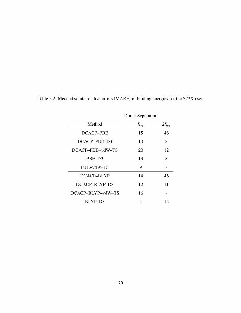
Table 5.2: Mean absolute relative errors (MARE) of binding energies for the S22X5 set.
Dimer Separation
Method Req 2Req
DCACP–PBE 15 46
DCACP–PBE–D3 10 8
DCACP–PBE+vdW–TS 20 12
PBE–D3 13 8
PBE+vdW–TS 9 -
DCACP–BLYP 14 46
DCACP–BLYP–D3 12 11
DCACP–BLYP+vdW–TS 16 -
BLYP–D3 4 12
70
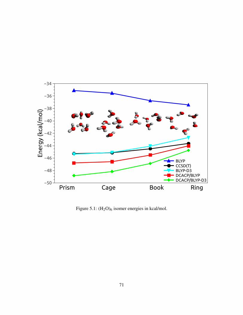
Ener
gy
(kca
l/m
ol)
−50
−48
−46
−44
−42
−40
−38
−36
−34
Prism Cage Book Ring
BLYPCCSD(T)BLYP-D3DCACP/BLYPDCACP/BLYP-D3
Figure 5.1: (H2O)6 isomer energies in kcal/mol.
71

Ener
gy
(kca
l/m
ol)
−49
−48
−47
−46
−45
−44
−43
−42
Prism Cage Book Ring
PBEDCACP/PBECCSD(T)DCACP/PBE-D3PBE-D3
Figure 5.2: (H2O)6 isomer energies in kcal/mol.
72
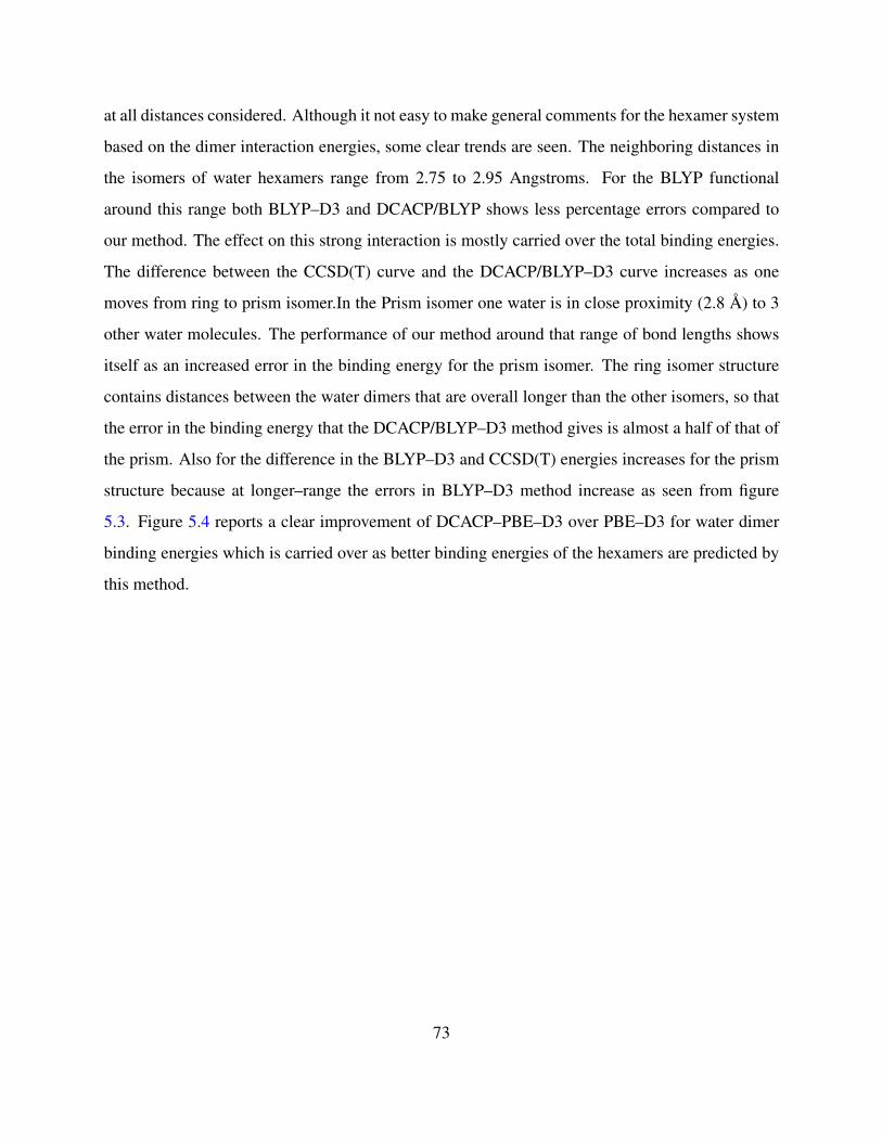
at all distances considered. Although it not easy to make general comments for the hexamer system
based on the dimer interaction energies, some clear trends are seen. The neighboring distances in
the isomers of water hexamers range from 2.75 to 2.95 Angstroms. For the BLYP functional
around this range both BLYP–D3 and DCACP/BLYP shows less percentage errors compared to
our method. The effect on this strong interaction is mostly carried over the total binding energies.
The difference between the CCSD(T) curve and the DCACP/BLYP–D3 curve increases as one
moves from ring to prism isomer.In the Prism isomer one water is in close proximity (2.8 A) to 3
other water molecules. The performance of our method around that range of bond lengths shows
itself as an increased error in the binding energy for the prism isomer. The ring isomer structure
contains distances between the water dimers that are overall longer than the other isomers, so that
the error in the binding energy that the DCACP/BLYP–D3 method gives is almost a half of that of
the prism. Also for the difference in the BLYP–D3 and CCSD(T) energies increases for the prism
structure because at longer–range the errors in BLYP–D3 method increase as seen from figure
5.3. Figure 5.4 reports a clear improvement of DCACP–PBE–D3 over PBE–D3 for water dimer
binding energies which is carried over as better binding energies of the hexamers are predicted by
this method.
73
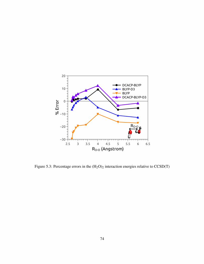
% E
rro
r
−30
−20
−10
0
10
20
RO-O (Angstrom)2.5 3 3.5 4 4.5 5 5.5 6 6.5
RO-O
DCACP-BLYPBLYP-D3BLYPDCACP-BLYP-D3
Figure 5.3: Percentage errors in the (H2O)2 interaction energies relative to CCSD(T)
74
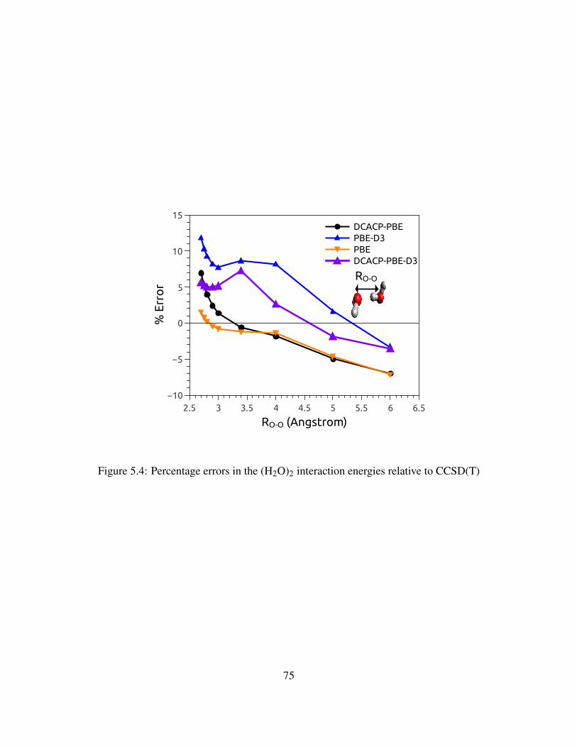
% E
rro
r
−10
−5
0
5
10
15
RO-O (Angstrom)2.5 3 3.5 4 4.5 5 5.5 6 6.5
RO-O
DCACP-PBEPBE-D3PBEDCACP-PBE-D3
Figure 5.4: Percentage errors in the (H2O)2 interaction energies relative to CCSD(T)
75
5.4 CONCLUSIONS
We proposed the DCACP+D method to correct the deficiencies in the original DCACP approach
to correct density functional for the missing dispersion interactions. DCACP+D method uses the
psedopotentials to correct for deficiencies in the employed functional and adds the dispersion en-
ergy using atom–atom type corrections. Grimme type (D3) dispersion correction methods works
better than the Tkatchenko–Scheffler method due to inclusion of C8/R8 terms. As seen from the
results for the S22 test set, the new method (DCACP+D) performs better for compared to the
original DCACPs for longer ranged distances where the DCACP interaction energies fall off too
quickly. The test cases show that when used with PBE functional the DCACP+D gives slightly
better interaction energies compared to the PBE–D3 method.
76
6.0 CORRECTING DENSITY FUNCTIONALS FOR DISPERSION INTERACTIONS
USING PSEUDOPOTENTIALS
This work was published as∗: Ozan Karalti, Xiaoge Su, Wissam A. Al–Saidi and Kenneth D.
Jordan Chemical Physics Letters, 591, (2014), 133†
6.1 INTRODUCTION
We present a two–channel dispersion–corrected atom–centered potential (DCACP) method for cor-
recting BLYP and PBE density functionals for long–range dispersion. The approach, designated
DCACP2, is tested on the S22X5 test set and on isomers of the water hexamer. The DCACP2
method provides a significantly improved description of the interaction energies at distances be-
yond Req than does the single–channel DCACP procedure.
The dispersion–corrected atom–centered potential (DCACP)12, 13 approach is one of sev-
eral methods12–29 designed to overcome the failure of commonly used density functional meth-
ods to describe dispersion interactions at distances beyond which there is appreciable overlap of
charge of the atoms or molecules of interest. The DCACP approach gives significantly improved
(compared to the uncorrected GGA functionals) interaction energies for a wide range of systems
near their equilibrium structures.12, 13, 50–55 However, the DCACP correction to the interaction en-
ergy falls off much more rapidly than R−6 with increasing distance between the monomers in a
∗Reproduced by permission of the Elsevier Science†O. K. prepared the publication and contributed all of the numerical data. X. S. contributed to the coding part.
77
dimer.54–56 In a study of isomers of the water hexamer we concluded that, at least when used
with the BLYP functional,47, 48 the DCACP method is correcting for limitations of the functional
in describing exchange-repulsion interaction as well as for dispersion interactions.55
The DCACP procedure modifies the electronic density by adding to the Hamiltonian atom–
centered non–local potentials of the form,
Vl(r,r′) =
l
∑m=-l
Ylm(r)pl(r;σ2)σ1pl(r′;σ2)Ylm(r
′), (6.1)
where Ylm denotes a spherical harmonic, and pl is a normalized projector defined as pl(r;σ2) ∝
rlexp[–r2/2σ22 ] . The correction potentials are of the same functional form as the non–local chan-
nels of the Goedecker–Teter–Hutter pseudopotentials.45 The parameter σ1 scales the magnitude
of the pseudopotential, and σ2 tunes the location of the projector’s maximum from the atom cen-
ter. In their application of this method, Roethlisberger and coworkers used the l = 3 channel, and
determined the σ1 and σ2 parameters by use of a penalty function that minimized the differences
between the DCACP and full CI or CCSD(T)46 energies and forces evaluated at the equilibrium
and midpoint geometries (the point where the interaction energy equals half that of the equilib-
rium value) for a small set of dimers. The DCACP method has been implemented for the PBE,9
BLYP47, 48 and Becke-Perdew47, 49 functionals.
In the present study we investigate an extension of the DCACP method that employs more than
one angular momentum channel in the correction potential. The motivation is that this increased
flexibility should better enable the procedure to correct for both exchange–repulsion errors as well
as for long–range dispersion, extending the range of geometries for which the method is useful.
The multiple channel DCACP method was originally introduced in Ref.56 where in an application
to (H2)2 three angular momentum channels (p, d and f ) were used to fit the H pseudopotential
to the full configuration–interaction energy curve. However, this three-channel H pseudopotential
was not published. In this study we extend the approach to C, N, and O employing the d and
f channels in the pseudopotential. The procedure is referred to as DCACP2 to indicate the use
of two channels to correct the interaction energies. As in Ref. 25, we use three channels for H,
although similar results would have been obtained had we used only two channels. We parametrize
78
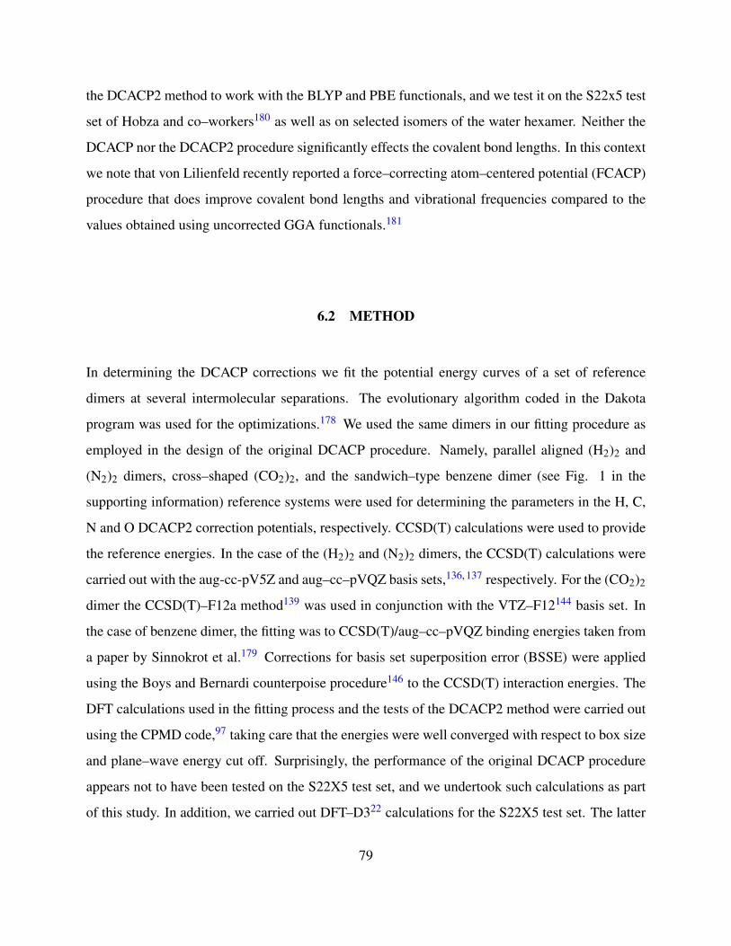
the DCACP2 method to work with the BLYP and PBE functionals, and we test it on the S22x5 test
set of Hobza and co–workers180 as well as on selected isomers of the water hexamer. Neither the
DCACP nor the DCACP2 procedure significantly effects the covalent bond lengths. In this context
we note that von Lilienfeld recently reported a force–correcting atom–centered potential (FCACP)
procedure that does improve covalent bond lengths and vibrational frequencies compared to the
values obtained using uncorrected GGA functionals.181
6.2 METHOD
In determining the DCACP corrections we fit the potential energy curves of a set of reference
dimers at several intermolecular separations. The evolutionary algorithm coded in the Dakota
program was used for the optimizations.178 We used the same dimers in our fitting procedure as
employed in the design of the original DCACP procedure. Namely, parallel aligned (H2)2 and
(N2)2 dimers, cross–shaped (CO2)2, and the sandwich–type benzene dimer (see Fig. 1 in the
supporting information) reference systems were used for determining the parameters in the H, C,
N and O DCACP2 correction potentials, respectively. CCSD(T) calculations were used to provide
the reference energies. In the case of the (H2)2 and (N2)2 dimers, the CCSD(T) calculations were
carried out with the aug-cc-pV5Z and aug–cc–pVQZ basis sets,136, 137 respectively. For the (CO2)2
dimer the CCSD(T)–F12a method139 was used in conjunction with the VTZ–F12144 basis set. In
the case of benzene dimer, the fitting was to CCSD(T)/aug–cc–pVQZ binding energies taken from
a paper by Sinnokrot et al.179 Corrections for basis set superposition error (BSSE) were applied
using the Boys and Bernardi counterpoise procedure146 to the CCSD(T) interaction energies. The
DFT calculations used in the fitting process and the tests of the DCACP2 method were carried out
using the CPMD code,97 taking care that the energies were well converged with respect to box size
and plane–wave energy cut off. Surprisingly, the performance of the original DCACP procedure
appears not to have been tested on the S22X5 test set, and we undertook such calculations as part
of this study. In addition, we carried out DFT–D322 calculations for the S22X5 test set. The latter
79
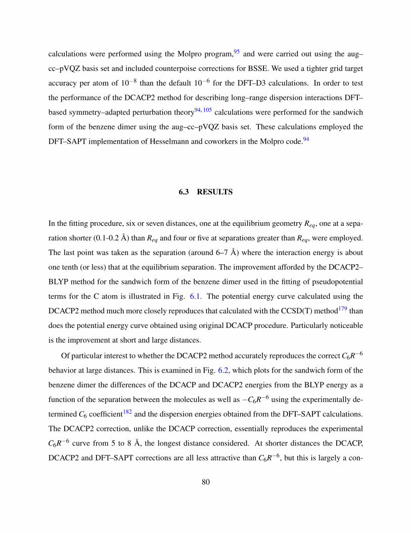
calculations were performed using the Molpro program,95 and were carried out using the aug–
cc–pVQZ basis set and included counterpoise corrections for BSSE. We used a tighter grid target
accuracy per atom of 10−8 than the default 10−6 for the DFT–D3 calculations. In order to test
the performance of the DCACP2 method for describing long–range dispersion interactions DFT–
based symmetry–adapted perturbation theory94, 105 calculations were performed for the sandwich
form of the benzene dimer using the aug–cc–pVQZ basis set. These calculations employed the
DFT–SAPT implementation of Hesselmann and coworkers in the Molpro code.94
6.3 RESULTS
In the fitting procedure, six or seven distances, one at the equilibrium geometry Req, one at a sepa-
ration shorter (0.1-0.2 A) than Req and four or five at separations greater than Req, were employed.
The last point was taken as the separation (around 6–7 A) where the interaction energy is about
one tenth (or less) that at the equilibrium separation. The improvement afforded by the DCACP2–
BLYP method for the sandwich form of the benzene dimer used in the fitting of pseudopotential
terms for the C atom is illustrated in Fig. 6.1. The potential energy curve calculated using the
DCACP2 method much more closely reproduces that calculated with the CCSD(T) method179 than
does the potential energy curve obtained using original DCACP procedure. Particularly noticeable
is the improvement at short and large distances.
Of particular interest to whether the DCACP2 method accurately reproduces the correct C6R−6
behavior at large distances. This is examined in Fig. 6.2, which plots for the sandwich form of the
benzene dimer the differences of the DCACP and DCACP2 energies from the BLYP energy as a
function of the separation between the molecules as well as −C6R−6 using the experimentally de-
termined C6 coefficient182 and the dispersion energies obtained from the DFT–SAPT calculations.
The DCACP2 correction, unlike the DCACP correction, essentially reproduces the experimental
C6R−6 curve from 5 to 8 A, the longest distance considered. At shorter distances the DCACP,
DCACP2 and DFT–SAPT corrections are all less attractive than C6R−6, but this is largely a con-
80
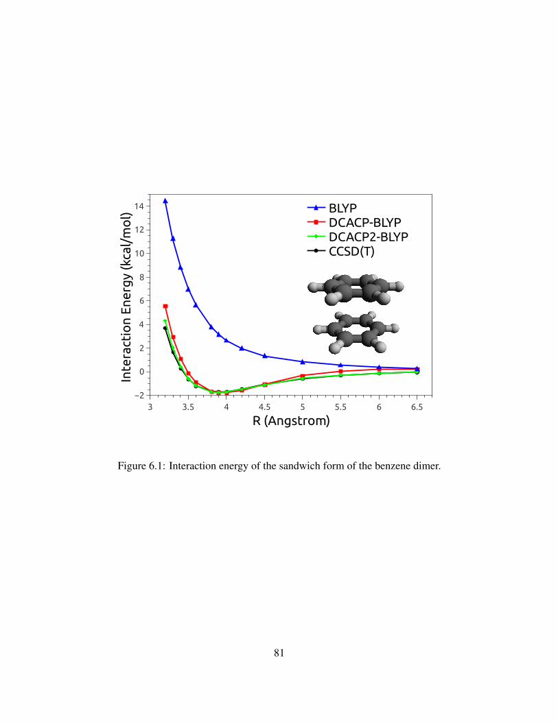
Inte
ract
ion
Ener
gy
(kca
l/m
ol)
−2
0
2
4
6
8
10
12
14
R (Angstrom)3 3.5 4 4.5 5 5.5 6 6.5
BLYPDCACP-BLYPDCACP2-BLYPCCSD(T)
Figure 6.1: Interaction energy of the sandwich form of the benzene dimer.
81

−5
−4
−3
−2
−1
0
4 5 6 7 8
Ener
gy
(kca
l/m
ol)
−10
−5
0
R (Angstrom)3 4 5 6 7 8
DCACP-corrDCACP2-corrSAPT-disp-C6R-6-exp
Figure 6.2: DCACP/BLYP corrections compared to exp. C6R−6 and DFT–SAPT dispersion.
82
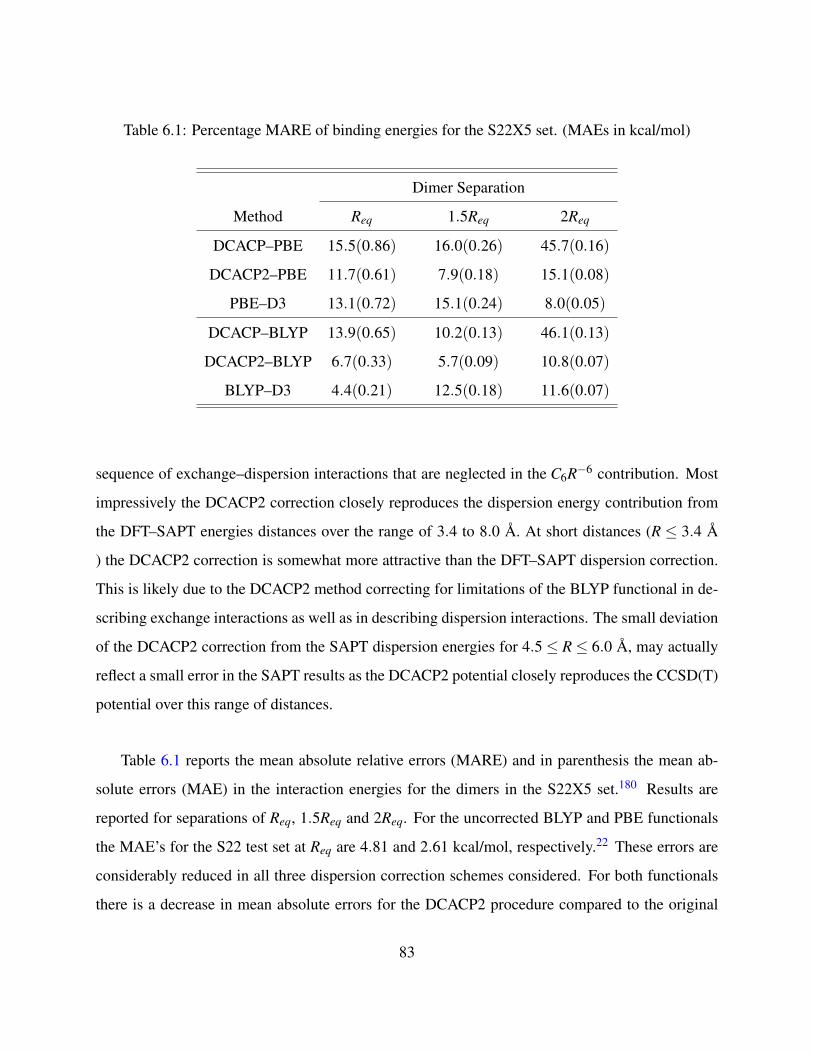
Table 6.1: Percentage MARE of binding energies for the S22X5 set. (MAEs in kcal/mol)
Dimer Separation
Method Req 1.5Req 2Req
DCACP–PBE 15.5(0.86) 16.0(0.26) 45.7(0.16)
DCACP2–PBE 11.7(0.61) 7.9(0.18) 15.1(0.08)
PBE–D3 13.1(0.72) 15.1(0.24) 8.0(0.05)
DCACP–BLYP 13.9(0.65) 10.2(0.13) 46.1(0.13)
DCACP2–BLYP 6.7(0.33) 5.7(0.09) 10.8(0.07)
BLYP–D3 4.4(0.21) 12.5(0.18) 11.6(0.07)
sequence of exchange–dispersion interactions that are neglected in the C6R−6 contribution. Most
impressively the DCACP2 correction closely reproduces the dispersion energy contribution from
the DFT–SAPT energies distances over the range of 3.4 to 8.0 A. At short distances (R ≤ 3.4 A
) the DCACP2 correction is somewhat more attractive than the DFT–SAPT dispersion correction.
This is likely due to the DCACP2 method correcting for limitations of the BLYP functional in de-
scribing exchange interactions as well as in describing dispersion interactions. The small deviation
of the DCACP2 correction from the SAPT dispersion energies for 4.5 ≤ R ≤ 6.0 A, may actually
reflect a small error in the SAPT results as the DCACP2 potential closely reproduces the CCSD(T)
potential over this range of distances.
Table 6.1 reports the mean absolute relative errors (MARE) and in parenthesis the mean ab-
solute errors (MAE) in the interaction energies for the dimers in the S22X5 set.180 Results are
reported for separations of Req, 1.5Req and 2Req. For the uncorrected BLYP and PBE functionals
the MAE’s for the S22 test set at Req are 4.81 and 2.61 kcal/mol, respectively.22 These errors are
considerably reduced in all three dispersion correction schemes considered. For both functionals
there is a decrease in mean absolute errors for the DCACP2 procedure compared to the original
83
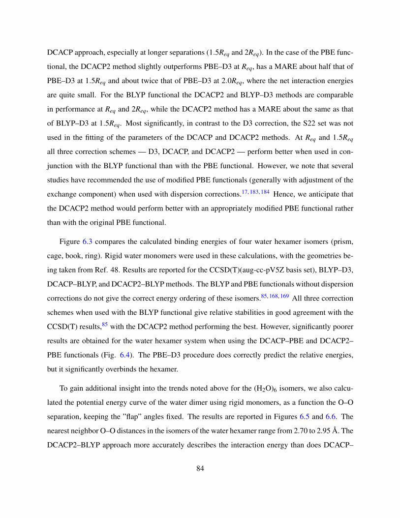
DCACP approach, especially at longer separations (1.5Req and 2Req). In the case of the PBE func-
tional, the DCACP2 method slightly outperforms PBE–D3 at Req, has a MARE about half that of
PBE–D3 at 1.5Req and about twice that of PBE–D3 at 2.0Req, where the net interaction energies
are quite small. For the BLYP functional the DCACP2 and BLYP–D3 methods are comparable
in performance at Req and 2Req, while the DCACP2 method has a MARE about the same as that
of BLYP–D3 at 1.5Req. Most significantly, in contrast to the D3 correction, the S22 set was not
used in the fitting of the parameters of the DCACP and DCACP2 methods. At Req and 1.5Req
all three correction schemes — D3, DCACP, and DCACP2 — perform better when used in con-
junction with the BLYP functional than with the PBE functional. However, we note that several
studies have recommended the use of modified PBE functionals (generally with adjustment of the
exchange component) when used with dispersion corrections.17, 183, 184 Hence, we anticipate that
the DCACP2 method would perform better with an appropriately modified PBE functional rather
than with the original PBE functional.
Figure 6.3 compares the calculated binding energies of four water hexamer isomers (prism,
cage, book, ring). Rigid water monomers were used in these calculations, with the geometries be-
ing taken from Ref. 48. Results are reported for the CCSD(T)(aug-cc-pV5Z basis set), BLYP–D3,
DCACP–BLYP, and DCACP2–BLYP methods. The BLYP and PBE functionals without dispersion
corrections do not give the correct energy ordering of these isomers.85, 168, 169 All three correction
schemes when used with the BLYP functional give relative stabilities in good agreement with the
CCSD(T) results,85 with the DCACP2 method performing the best. However, significantly poorer
results are obtained for the water hexamer system when using the DCACP–PBE and DCACP2–
PBE functionals (Fig. 6.4). The PBE–D3 procedure does correctly predict the relative energies,
but it significantly overbinds the hexamer.
To gain additional insight into the trends noted above for the (H2O)6 isomers, we also calcu-
lated the potential energy curve of the water dimer using rigid monomers, as a function the O–O
separation, keeping the ”flap” angles fixed. The results are reported in Figures 6.5 and 6.6. The
nearest neighbor O–O distances in the isomers of the water hexamer range from 2.70 to 2.95 A. The
DCACP2–BLYP approach more accurately describes the interaction energy than does DCACP–
84
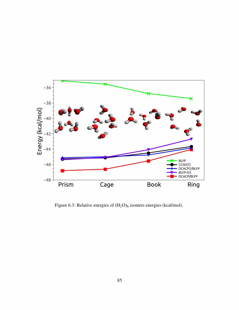
Ener
gy
(kca
l/m
ol)
−48
−46
−44
−42
−40
−38
−36
Prism Cage Book Ring
BLYPCCSD(T)DCACP2/BLYPBLYP-D3DCACP/BLYP
Figure 6.3: Relative energies of (H2O)6 isomers energies (kcal/mol).
85
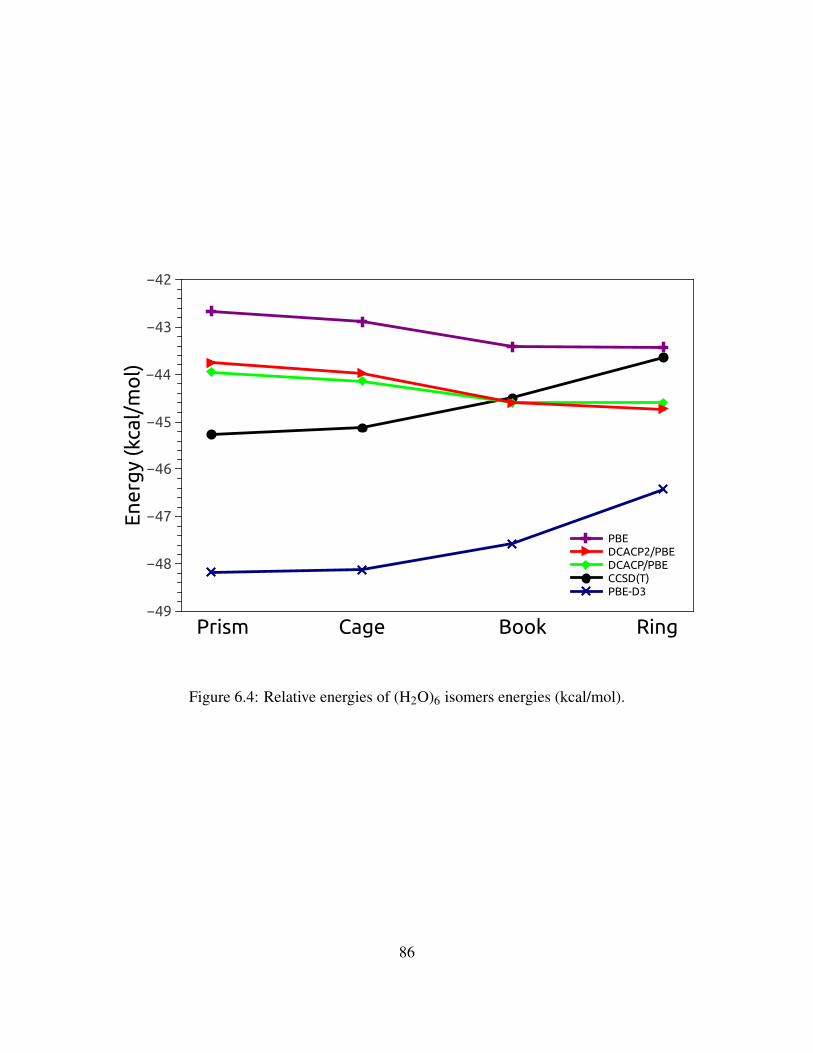
Ener
gy
(kca
l/m
ol)
−49
−48
−47
−46
−45
−44
−43
−42
Prism Cage Book Ring
PBEDCACP2/PBEDCACP/PBECCSD(T)PBE-D3
Figure 6.4: Relative energies of (H2O)6 isomers energies (kcal/mol).
86
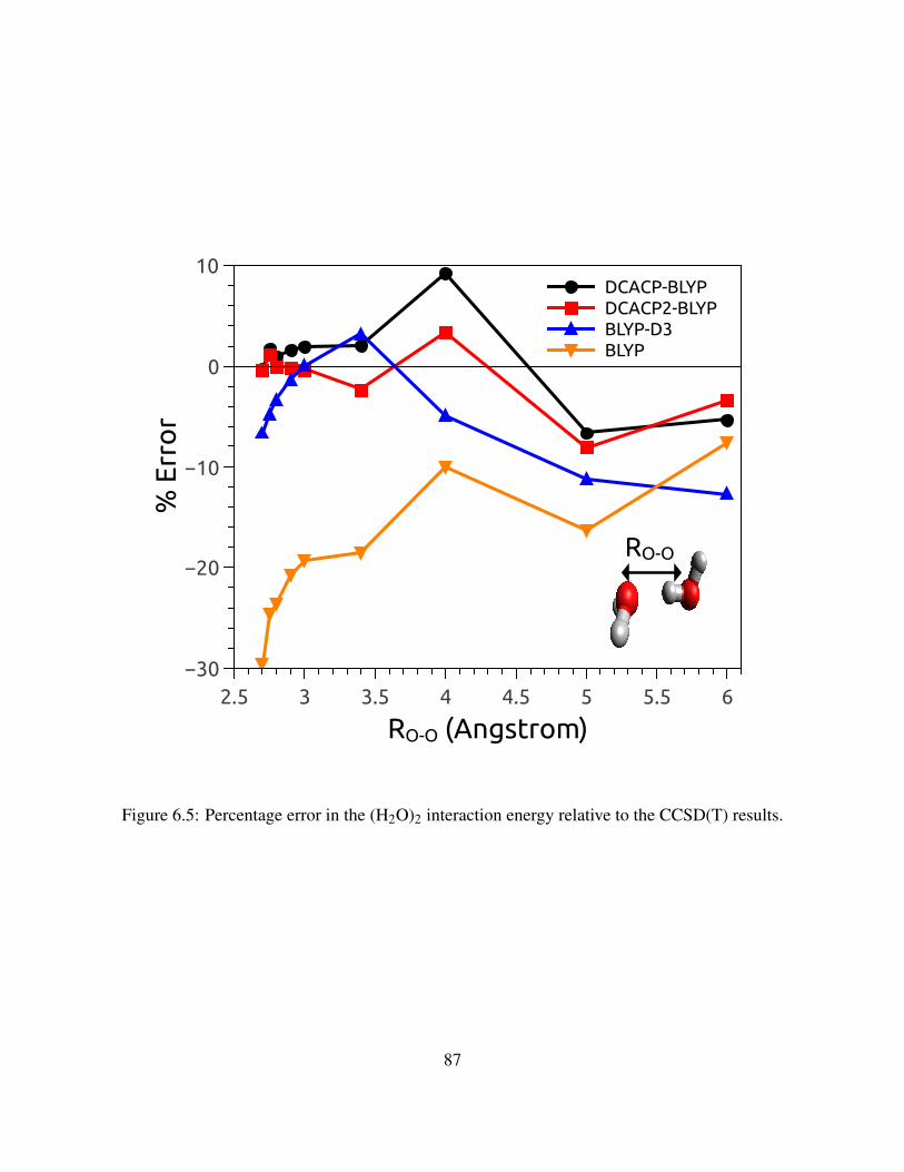
% E
rro
r
−30
−20
−10
0
10
RO-O (Angstrom)2.5 3 3.5 4 4.5 5 5.5 6
DCACP-BLYPDCACP2-BLYPBLYP-D3BLYP
RO-O
Figure 6.5: Percentage error in the (H2O)2 interaction energy relative to the CCSD(T) results.
87
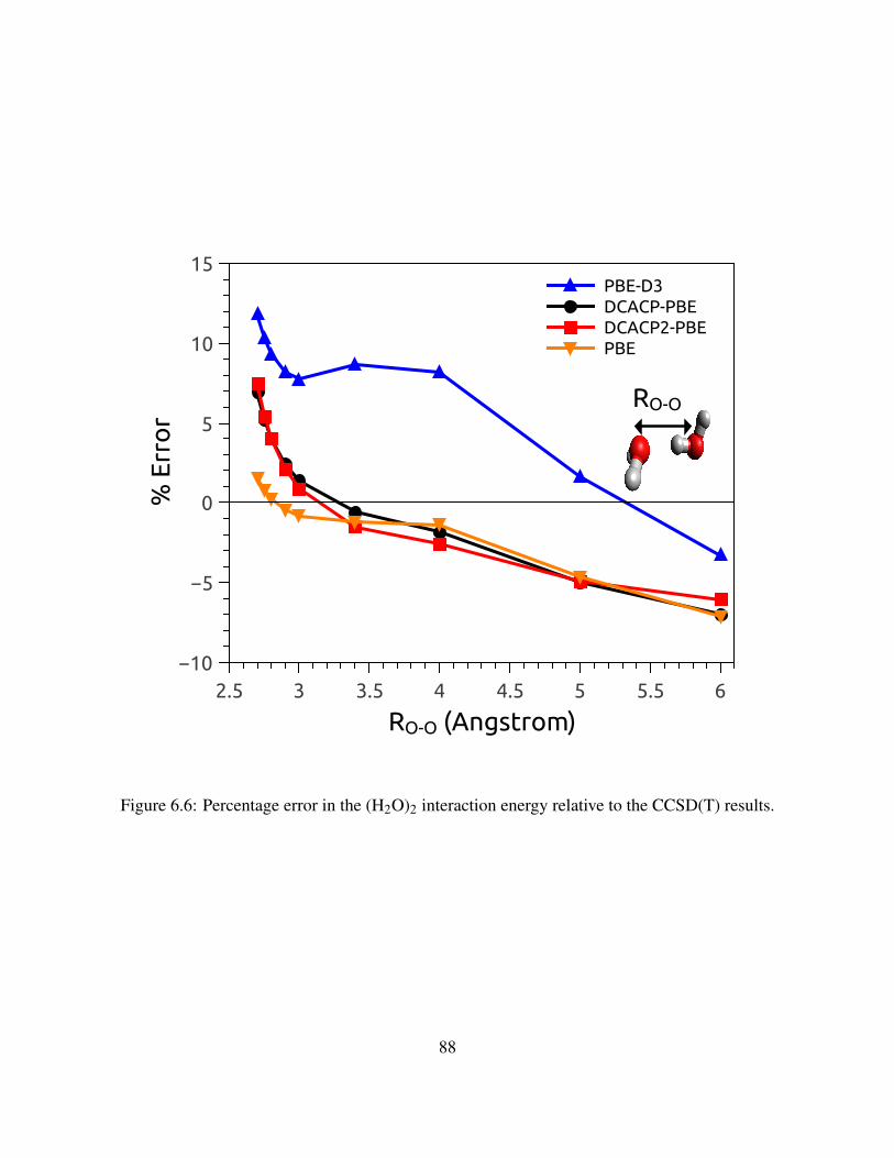
% E
rro
r
−10
−5
0
5
10
15
RO-O (Angstrom)2.5 3 3.5 4 4.5 5 5.5 6
PBE-D3DCACP-PBEDCACP2-PBEPBE
RO-O
Figure 6.6: Percentage error in the (H2O)2 interaction energy relative to the CCSD(T) results.
88
BLYP for O–O distances ranging from 2.2 to about 5.2 A. However, with the PBE functional, the
DCACP2 and DCACP methods give nearly identical potential energy curves for the water dimer.
6.4 CONCLUSIONS
A two–channel DCACP method, designated DCACP2, has been developed for H, C, N, and O. The
implementation has been made for both the BLYP and PBE density functionals through the addi-
tion of terms to the Goedecker–Teter–Hutter type pseudopotentials. The DCACP2 method, per-
forms significantly better than the one–channel DCACP approach on the S22X5 test set, with the
improvement being particularly notable with the BLYP functional. Most importantly, the DCACP2
method provides a much better description of the interaction energies at distances beyond Req than
does the original DCACP procedure. The DCACP2–BLYP procedure gives absolute and relative
binding energies of the ring, cage, prism and book isomers of the (H2O)6 in excellent agreement
with the results of CCSD(T) calculations. Work is underway in our group to provide parameters
for the DCACP2 procedure for a wider range of elements.
6.5 ACKNOWLEDGMENTS
This research was carried out with the support of a grant CHE–1111235 from the National Science
Foundation. The calculations were performed on computers in University of Pittsburgh’s Center
for Simulation and Modeling.
89
7.0 CONCLUSIONS
The first part of thesis provides an overview of most of the methods used for correcting density
functional theory methods for long–range dispersion interactions. Tests with various systems in
Chapters 2 and 3 shows that all of these methods clearly provides better interaction energies com-
pared to what their uncorrected density functional gives. Among those dispersion corrected meth-
ods DFT-D3’s good accuracy in predicting the longer–ranged interactions and simplicity and ac-
curacy of interaction energies at the equilibrium lengths provided by the DCACP methods catches
attention. The detailed test with the isomers of the water hexamer suggests that when used with
the BLYP functional the original implementation of the DCACPs not only corrects for limitations
of the functional in describing dispersion interactions but also corrects for exchange-repulsion in-
teractions. In chapters 5 and 6 we provided two methods for improving the DCACP methodology.
First proposal is to fit the DCACPs to non–dispersion terms in the interaction energy and then aug-
ment it with DFT–D3 type dispersion energies. The DCACP+D method combined with the PBE
functional improves the accuracy in the interaction energies near equilibrium points and also solves
the wrong asypmtotic decay behavior of the original DCACPs. The DCACP2 scheme proposed in
chapter 6 uses two channels in the pseudopotential rather than a single f channel for modeling the
dispersion interactions. The DCACP2 method, performs significantly better than the one–channel
DCACP approach on the S22X5 test set, with the improvement being particularly notable with the
BLYP functional. Most importantly, the DCACP2 method provides a much better description of
the interaction energies at distances beyond Req than does the original DCACP procedure. The
DCACP2–BLYP procedure gives absolute and relative binding energies of the ring, cage, prism
and book isomers of the (H2O)6 in excellent agreement with the results of CCSD(T) calculations.
90

Work is underway in our group to provide parameters for the DCACP2 procedure for a wider range
of elements.
91
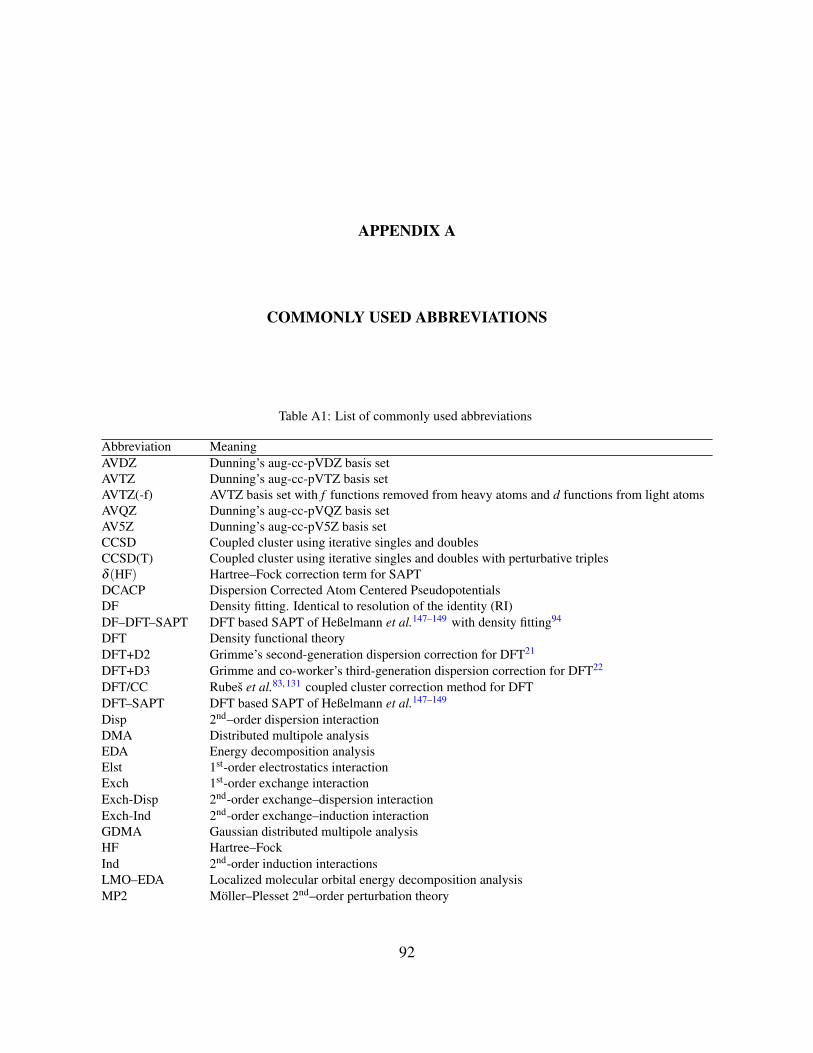
APPENDIX A
COMMONLY USED ABBREVIATIONS
Table A1: List of commonly used abbreviations
Abbreviation MeaningAVDZ Dunning’s aug-cc-pVDZ basis setAVTZ Dunning’s aug-cc-pVTZ basis setAVTZ(-f) AVTZ basis set with f functions removed from heavy atoms and d functions from light atomsAVQZ Dunning’s aug-cc-pVQZ basis setAV5Z Dunning’s aug-cc-pV5Z basis setCCSD Coupled cluster using iterative singles and doublesCCSD(T) Coupled cluster using iterative singles and doubles with perturbative triplesδ (HF) Hartree–Fock correction term for SAPTDCACP Dispersion Corrected Atom Centered PseudopotentialsDF Density fitting. Identical to resolution of the identity (RI)DF–DFT–SAPT DFT based SAPT of Heßelmann et al.147–149 with density fitting94
DFT Density functional theoryDFT+D2 Grimme’s second-generation dispersion correction for DFT21
DFT+D3 Grimme and co-worker’s third-generation dispersion correction for DFT22
DFT/CC Rubes et al.83, 131 coupled cluster correction method for DFTDFT–SAPT DFT based SAPT of Heßelmann et al.147–149
Disp 2nd–order dispersion interactionDMA Distributed multipole analysisEDA Energy decomposition analysisElst 1st-order electrostatics interactionExch 1st-order exchange interactionExch-Disp 2nd-order exchange–dispersion interactionExch-Ind 2nd-order exchange–induction interactionGDMA Gaussian distributed multipole analysisHF Hartree–FockInd 2nd-order induction interactionsLMO–EDA Localized molecular orbital energy decomposition analysisMP2 Moller–Plesset 2nd–order perturbation theory
92

MBPTn Many-body perturbation theory through order nRI Resolution of the identity. Identical to density fitting (DF).SAPT Symmetry-adapted perturbation theorySAPT(DFT) DFT based SAPT of Misquitta et al.105, 185, 186
Tr-AVTZ Truncated AVTZ basis set as described in Section 2.2vdW-TS Tkatchenko and Sheffler type dispersion correctionXC Exchange–Correlation
93

APPENDIX B
SUPPORTING INFORMATION FOR CHAPTER 6
94
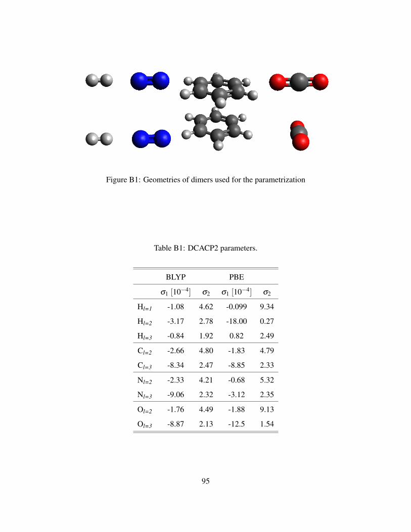
Figure B1: Geometries of dimers used for the parametrization
Table B1: DCACP2 parameters.
BLYP PBE
σ1 [10−4] σ2 σ1 [10−4] σ2
Hl=1 -1.08 4.62 -0.099 9.34
Hl=2 -3.17 2.78 -18.00 0.27
Hl=3 -0.84 1.92 0.82 2.49
Cl=2 -2.66 4.80 -1.83 4.79
Cl=3 -8.34 2.47 -8.85 2.33
Nl=2 -2.33 4.21 -0.68 5.32
Nl=3 -9.06 2.32 -3.12 2.35
Ol=2 -1.76 4.49 -1.88 9.13
Ol=3 -8.87 2.13 -12.5 1.54
95
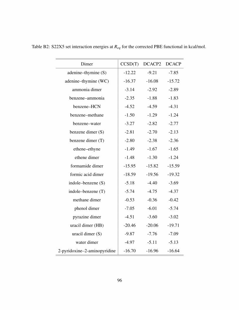
Table B2: S22X5 set interaction energies at Req for the corrected PBE functional in kcal/mol.
Dimer CCSD(T) DCACP2 DCACP
adenine–thymine (S) -12.22 -9.21 -7.85
adenine–thymine (WC) -16.37 -16.08 -15.72
ammonia dimer -3.14 -2.92 -2.89
benzene–ammonia -2.35 -1.88 -1.83
benzene–HCN -4.52 -4.59 -4.31
benzene–methane -1.50 -1.29 -1.24
benzene–water -3.27 -2.82 -2.77
benzene dimer (S) -2.81 -2.70 -2.13
benzene dimer (T) -2.80 -2.38 -2.36
ethene–ethyne -1.49 -1.67 -1.65
ethene dimer -1.48 -1.30 -1.24
formamide dimer -15.95 -15.82 -15.59
formic acid dimer -18.59 -19.56 -19.32
indole–benzene (S) -5.18 -4.40 -3.69
indole–benzene (T) -5.74 -4.75 -4.37
methane dimer -0.53 -0.36 -0.42
phenol dimer -7.05 -6.01 -5.74
pyrazine dimer -4.51 -3.60 -3.02
uracil dimer (HB) -20.46 -20.06 -19.71
uracil dimer (S) -9.87 -7.76 -7.09
water dimer -4.97 -5.11 -5.13
2-pyridoxine–2-aminopyridine -16.70 -16.96 -16.64
96
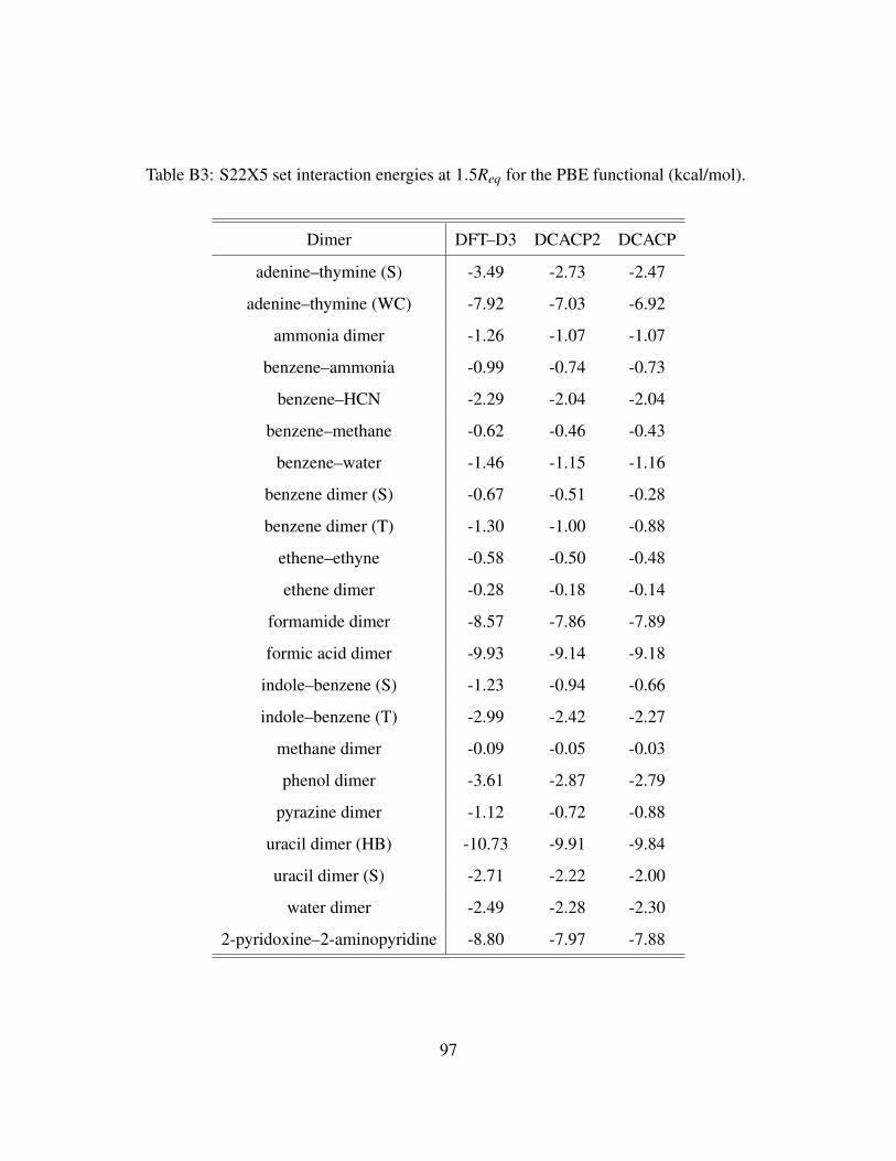
Table B3: S22X5 set interaction energies at 1.5Req for the PBE functional (kcal/mol).
Dimer DFT–D3 DCACP2 DCACP
adenine–thymine (S) -3.49 -2.73 -2.47
adenine–thymine (WC) -7.92 -7.03 -6.92
ammonia dimer -1.26 -1.07 -1.07
benzene–ammonia -0.99 -0.74 -0.73
benzene–HCN -2.29 -2.04 -2.04
benzene–methane -0.62 -0.46 -0.43
benzene–water -1.46 -1.15 -1.16
benzene dimer (S) -0.67 -0.51 -0.28
benzene dimer (T) -1.30 -1.00 -0.88
ethene–ethyne -0.58 -0.50 -0.48
ethene dimer -0.28 -0.18 -0.14
formamide dimer -8.57 -7.86 -7.89
formic acid dimer -9.93 -9.14 -9.18
indole–benzene (S) -1.23 -0.94 -0.66
indole–benzene (T) -2.99 -2.42 -2.27
methane dimer -0.09 -0.05 -0.03
phenol dimer -3.61 -2.87 -2.79
pyrazine dimer -1.12 -0.72 -0.88
uracil dimer (HB) -10.73 -9.91 -9.84
uracil dimer (S) -2.71 -2.22 -2.00
water dimer -2.49 -2.28 -2.30
2-pyridoxine–2-aminopyridine -8.80 -7.97 -7.88
97
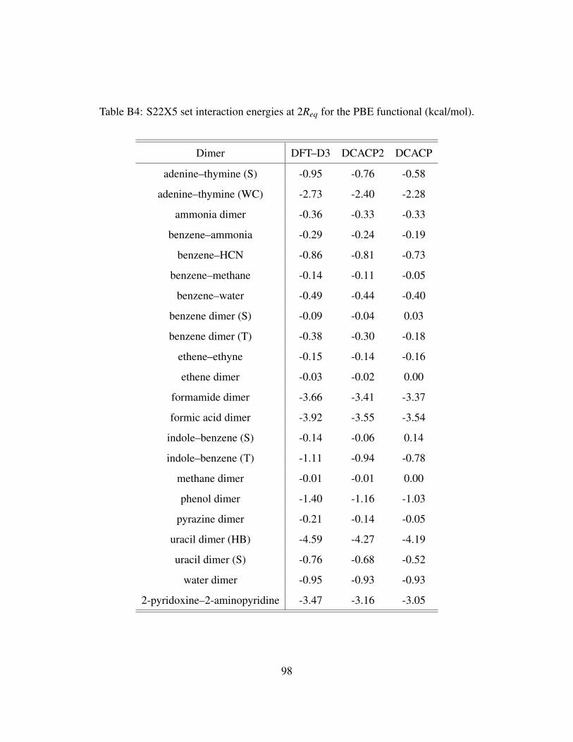
Table B4: S22X5 set interaction energies at 2Req for the PBE functional (kcal/mol).
Dimer DFT–D3 DCACP2 DCACP
adenine–thymine (S) -0.95 -0.76 -0.58
adenine–thymine (WC) -2.73 -2.40 -2.28
ammonia dimer -0.36 -0.33 -0.33
benzene–ammonia -0.29 -0.24 -0.19
benzene–HCN -0.86 -0.81 -0.73
benzene–methane -0.14 -0.11 -0.05
benzene–water -0.49 -0.44 -0.40
benzene dimer (S) -0.09 -0.04 0.03
benzene dimer (T) -0.38 -0.30 -0.18
ethene–ethyne -0.15 -0.14 -0.16
ethene dimer -0.03 -0.02 0.00
formamide dimer -3.66 -3.41 -3.37
formic acid dimer -3.92 -3.55 -3.54
indole–benzene (S) -0.14 -0.06 0.14
indole–benzene (T) -1.11 -0.94 -0.78
methane dimer -0.01 -0.01 0.00
phenol dimer -1.40 -1.16 -1.03
pyrazine dimer -0.21 -0.14 -0.05
uracil dimer (HB) -4.59 -4.27 -4.19
uracil dimer (S) -0.76 -0.68 -0.52
water dimer -0.95 -0.93 -0.93
2-pyridoxine–2-aminopyridine -3.47 -3.16 -3.05
98
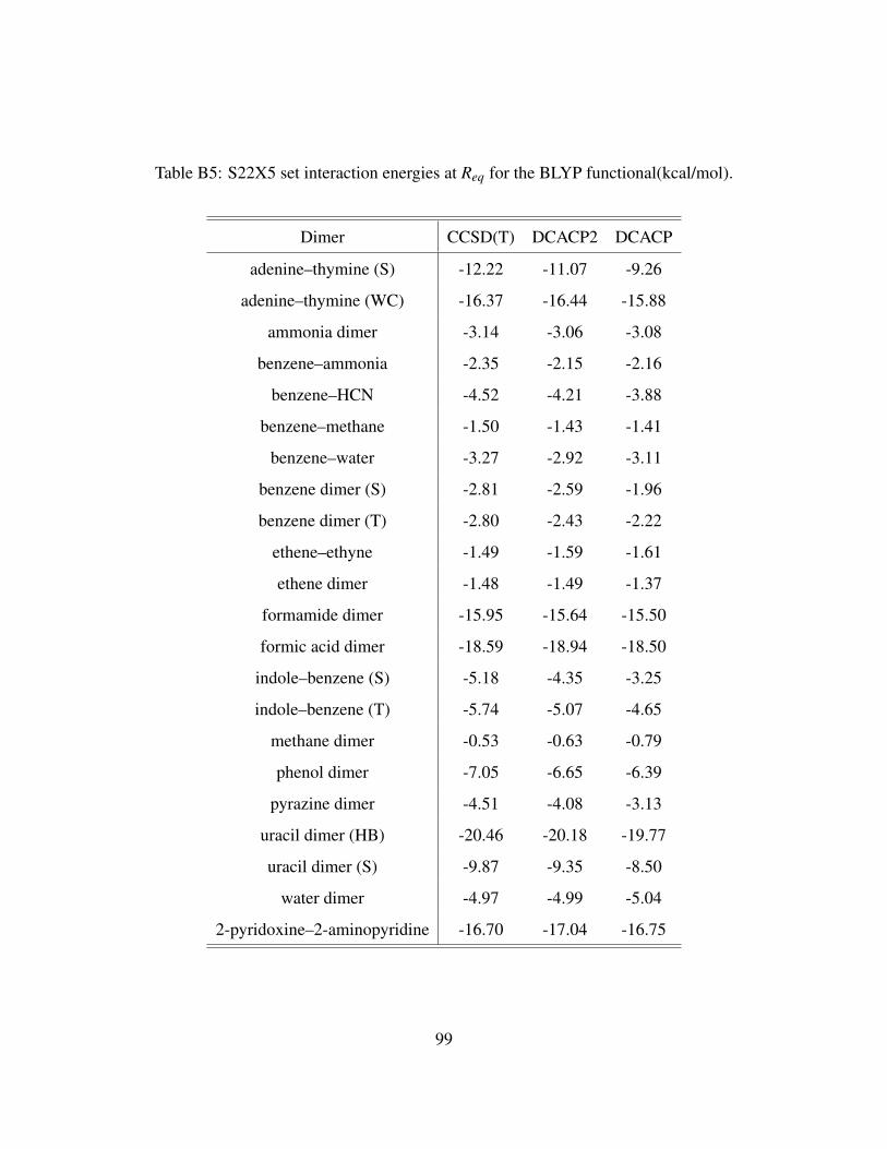
Table B5: S22X5 set interaction energies at Req for the BLYP functional(kcal/mol).
Dimer CCSD(T) DCACP2 DCACP
adenine–thymine (S) -12.22 -11.07 -9.26
adenine–thymine (WC) -16.37 -16.44 -15.88
ammonia dimer -3.14 -3.06 -3.08
benzene–ammonia -2.35 -2.15 -2.16
benzene–HCN -4.52 -4.21 -3.88
benzene–methane -1.50 -1.43 -1.41
benzene–water -3.27 -2.92 -3.11
benzene dimer (S) -2.81 -2.59 -1.96
benzene dimer (T) -2.80 -2.43 -2.22
ethene–ethyne -1.49 -1.59 -1.61
ethene dimer -1.48 -1.49 -1.37
formamide dimer -15.95 -15.64 -15.50
formic acid dimer -18.59 -18.94 -18.50
indole–benzene (S) -5.18 -4.35 -3.25
indole–benzene (T) -5.74 -5.07 -4.65
methane dimer -0.53 -0.63 -0.79
phenol dimer -7.05 -6.65 -6.39
pyrazine dimer -4.51 -4.08 -3.13
uracil dimer (HB) -20.46 -20.18 -19.77
uracil dimer (S) -9.87 -9.35 -8.50
water dimer -4.97 -4.99 -5.04
2-pyridoxine–2-aminopyridine -16.70 -17.04 -16.75
99

Table B6: S22X5 set interaction energies at 1.5Req for the BLYP functional (kcal/mol).
Dimer DFT–D3 DCACP2 DCACP
adenine–thymine (S) -3.49 -3.34 -2.90
adenine–thymine (WC) -7.92 -7.24 -7.29
ammonia dimer -1.26 -1.03 -1.11
benzene–ammonia -0.99 -0.75 -0.79
benzene–HCN -2.29 -2.01 -2.05
benzene–methane -0.62 -0.47 -0.46
benzene–water -1.46 -1.12 -1.20
benzene dimer (S) -0.67 -0.56 -0.31
benzene dimer (T) -1.30 -1.12 -1.02
ethene–ethyne -0.58 -0.48 -0.47
ethene dimer -0.28 -0.21 -0.20
formamide dimer -8.57 -7.97 -8.14
formic acid dimer -9.93 -9.51 -9.69
indole–benzene (S) -1.23 -1.04 -0.75
indole–benzene (T) -2.99 -2.60 -2.51
methane dimer -0.09 -0.04 -0.02
phenol dimer -3.61 -3.21 -3.30
pyrazine dimer -1.12 -1.04 -0.88
uracil dimer (HB) -10.73 -10.34 -10.43
uracil dimer (S) -2.71 -2.47 -2.29
water dimer -2.49 -2.30 -2.43
2-pyridoxine–2-aminopyridine -8.80 -8.31 -8.36
100
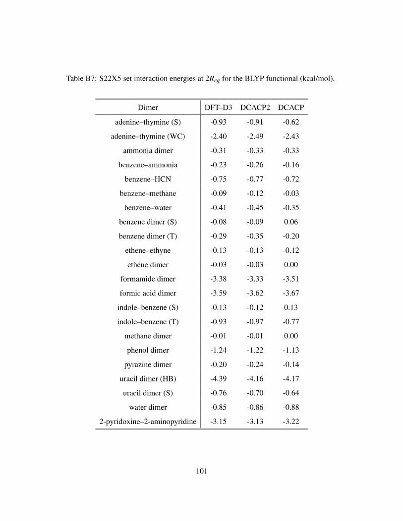
Table B7: S22X5 set interaction energies at 2Req for the BLYP functional (kcal/mol).
Dimer DFT–D3 DCACP2 DCACP
adenine–thymine (S) -0.93 -0.91 -0.62
adenine–thymine (WC) -2.40 -2.49 -2.43
ammonia dimer -0.31 -0.33 -0.33
benzene–ammonia -0.23 -0.26 -0.16
benzene–HCN -0.75 -0.77 -0.72
benzene–methane -0.09 -0.12 -0.03
benzene–water -0.41 -0.45 -0.35
benzene dimer (S) -0.08 -0.09 0.06
benzene dimer (T) -0.29 -0.35 -0.20
ethene–ethyne -0.13 -0.13 -0.12
ethene dimer -0.03 -0.03 0.00
formamide dimer -3.38 -3.33 -3.51
formic acid dimer -3.59 -3.62 -3.67
indole–benzene (S) -0.13 -0.12 0.13
indole–benzene (T) -0.93 -0.97 -0.77
methane dimer -0.01 -0.01 0.00
phenol dimer -1.24 -1.22 -1.13
pyrazine dimer -0.20 -0.24 -0.14
uracil dimer (HB) -4.39 -4.16 -4.17
uracil dimer (S) -0.76 -0.70 -0.64
water dimer -0.85 -0.86 -0.88
2-pyridoxine–2-aminopyridine -3.15 -3.13 -3.22
101
APPENDIX C
ADSORPTION OF A WATER MOLECULE ON THE MGO(100) SURFACE AS DESCRIBED BYCLUSTER AND SLAB MODELS
This work was published as∗: Ozan Karalti, Dario Alfe, Michael J. Gillan and Kenneth D. Jordan PhysicalChemistry Chemical Physics, 14, (2012), 7846–7853†
C.1 INTRODUCTION
The interaction of a water molecule with the (100) surface of MgO as described by cluster models is studied usingMP2, coupled MP2 (MP2C) and symmetry–adapted perturbation theory (SAPT) methods. In addition diffusion MonteCarlo (DMC) results are presented for several slab models as well as for the smallest, 2X2 cluster model. For the 2X2model it is found that the MP2C, DMC, and CCSD(T) methods all give nearly the same potential energy curve for thewater–cluster interaction, whereas the potential from the SAPT calculations differs slightly from the potentials of theother methods. The interaction of the water molecule with the cluster models of the MgO(100) surface is weakenedupon expanding the number of layers from one to two and also upon expanding the description of the layers from2X2 to 4X4 to 6X6. The SAPT calculations reveal that both these expansions of the cluster model are accompaniedby reductions in the magnitudes of the induction and dispersion constributions. The best estimate of the energy forbinding an isolated water model to the surface obtained from the cluster model calculations is in good agreement withthat obtained from the DMC calculations using a 2–layer slab model with periodic boundary conditions.
The adsorption of atoms and molecules on surfaces is of fundamental importance in a wide range of pro-cesses. MgO is an important component of the Earth’s subsurface and is used as a constituent in some superconductersand glasses as well as a catalyst. The nature of water adsorption on the MgO(100) surface has attracted considerableattention, being the subject of several experimental and theoretical studies.187–195 It appears that even at low cover-ages, molecularly adsorbed water is H–bonded to surface OH groups resulting from water dissociation and, as a result,an experimental value for the interaction energy of an isolated water molecule with the surface is not available. On thecomputational side, the water/MgO system has been investigated using semi–empirical methods,194 density functionaltheory (DFT),187 a mixed Hatree-Fock/coupled–cluster procedure combined with an embedded cluster model,190 anda study of the quantum nuclear effects on the adsorption energy.188
In the present work, we calculate the interaction energy between a water monomer and various cluster models ofthe MgO(100) surface. The methods used include density–fitted Moller–Plesset second–order perturbation theory (DF-
∗Reproduced by permission of the PCCP Owner Societies†D. A. contributed the QMC calculations and O. K. contributed the rest of the publication.
102
MP2),196, 197 density–fitted coupled MP2 (DF-MP2C),92, 142 and explicitly correlated DF–MP2 (DF–MP2–F12),138
DF–MP2C (DF-MP2C–F12), and CCSD(T) (CCSD(T)-F12).138, 140 In addition, calculations using the wavefunction–based166, 198 and density–fitted density–functional theory–based94 symmetry–adapted perturbation theory (SAPT) arecarried out. These are referred to as WF-SAPT and DFT-SAPT, respectively. The SAPT calculations are particularlyuseful for elucidating the factors at play in the adsorption of the water monomer as they provide physical dissectionsof the net interaction into electrostatics, exchange-repulsion, induction, and dispersion contributions. This informationshould prove especially valuable in designing force fields for simulating water on the MgO(100) surface. Due to thecomputational cost, the coupled cluster and WF–SAPT methods were applied only to the smallest cluster model.
In addition to the methods discussed above, the interaction energy between water and the MgO(100) surfacewas calculated using the diffusion Monte Carlo (DMC) method together with slab models and periodic boundaryconditions. For comparative purposes the DMC model was also applied to a water monomer interacting with thesmallest cluster model of the surface.
C.2 COMPUTATIONAL DETAILS
The MgO cluster models considered are single–layer 2X2, 4X4, and 6X6, and double–layer 4X4 (the nXn nomen-clature indicates that the cluster contains n rows of n atoms in the layer). The lattice constant used in the geometriesof the (MgO)n clusters were taken from a slab–model optimized with DFT-PBE using the VASP code.134 The single–layer cluster models of the bare surface have D2h symmetry and the double-layer cluster model have D2d symmetry.All nearest neighbor MgO bond lengths are 2.115 A. With one exception , described below, the geometry of the watermonomer (OH bond lengths of 0.989 A and HOH bond angle of 103.2 ◦ ) was also taken from a DFT-PBE optimizedgeometry, without allowing the Mg and O atoms of slabs to move, as was the orientation of the monomer relative tothe surface (see Fig. C1).
Due to the computational cost, WF–SAPT calculations were carried out only for the 2X2 cluster model, and themain approach for analyzing the interaction energies for the sequence of cluster models is the DFT–SAPT method.This method and the closely related SAPT(DFT) method of Szalewicz and co–workers105 determine the electrostaticand exchange–repulsion contributions to the interaction energy from integrals over the Coulomb operator evaluatedusing Kohn–Sham orbitals. Thus these approaches are free of the problems inherent in evaluating exchange–repulsionusing common density functional methods. The induction and dispersion contributions were calculated using responsefunctions from time–dependent DFT. The DFT–SAPT calculations made use of the LPBE0AC functional,94 whichreplaces the 25% Hartree–Fock exchange of the PBE0 functional34 with the 25% localized Hartree–Fock exchange ofSala and Gorling106 and includes an asymptotic correction.199 The correction scheme requires ionization potentialsof the fragments. For water the experimental IP reported in the NIST Chemistry Web Book,150 was used, and for the(MgO)n clusters, Koopmans’ theorem IP’s from Hartree–Fock calculations with the same basis set as employed in theDFT–SAPT calculations were used.
For the single–layer 2X2 and 4X4 cluster models, the DFT–SAPT calculations were performed using the aug–cc–pVQZ basis set137 on all atoms. For the double–layer 4X4 model, a mixed aug–cc–pVQZ/aug–cc–pVDZ136 basisset was used. This was generated by employing the aug–cc–pVQZ basis set for the water molecule and the twoclosest magnesium and two closest oxygen atoms in the top layer (the atoms marked by Xs in Fig. C1), with theaug–cc–pVDZ basis set being used for the remaining atoms. For the monomer SCF calculations and for the evaluationof the first–order electrostatics (E(1)
Elst ) and exhange (E(1)Exch) interactions, and the second–order induction (E(2)
Ind) and
exchange-induction (E(2)Ex−Ind) terms the cc–pVQZ JK–fitting set of Weigend109 was used for the oxygen and hydrogen
atoms, and the MP2-fitting set of Weigend and co–workers110 was used for the magnesium atoms. For the second-order dispersion and exchange-dispersion terms, the aug–cc–pVQZ MP2–fitting set of Weigend and co–workers110
was used for all atoms. In the case of the mixed basis set calculations double–zeta versions of the fitting sets wereused on the atoms employing the aug–cc–pVDZ basis sets.
The DF–MP2 and DF–MP2C calculations were carried out using the same basis sets and auxiliary fitting sets as
103

Figure C1: Geometry representing a water molecule on a 6X6 (MgO)18.
used in the DFT–SAPT calculations (the mixed basis set described above was used for the single–layer 6X6 clustermodel). These two approaches and the CCSD(T) method were also used in combination with F12a corrections.139
The F12a calculations used the cc–pVQZ–F12 (VQZ–F12) basis sets of Peterson and co-workers144 for the single–layer 2X2 and 4X4 cluster models and a combination of the cc–pVDZ–F12 (VDZ–F12) and VQZ–F12 basis sets forthe larger clusters following the same strategy described above for the DFT–SAPT calculations. For the oxygen andhydrogen atoms, the auxiliary basis sets implemented in MOLPRO2010.1 were used.109 For the magnesium atoms,the cc–pVDZ and cc–pVQZ MP2–fitting sets of Weigend and co-workers were used as the auxiliary basis sets for thecalculations using the VDZ-F12 and VQZ-F12 basis sets, respectively. The various MP2 and CCSD(T) calculationswere carried out with the non–valence core orbitals frozen. All calculations other than the quantum Monte Carlocalculations were performed with the MOLPRO2010.1 package.95
In reporting the results of the SAPT calculations the dispersion and exchange–dispersion contributions werecombined as were the induction, exchange–induction and δ (HF) contributions.94 In the SAPT procedure the inductionand exchange–induction contributions are calculated to second–order in the intermolecular interaction. The higherorder induction and exchange–induction interactions are accounted for by the so–called δ (HF) term.94
The quantum Monte Carlo calculations were performed with the CASINO code,200 using the diffusion MonteCarlo (DMC) method, together with trial wavefunctions that enforce fixed nodal surfaces.201 The trial wavefunctionsemployed were of the Slater–Jastrow type:
ΨT (R) = D↑D↓eJ , ( C.1)
where D↑ and D↓ are Slater determinants of up- and down–spin single–electron orbitals, and eJ is a Jastrow fac-tor, which is the exponential of a sum of one-body (electron–nucleus), two-body (electron–electron), and three body(electron–electron-nucleus) terms, that are parametrized functions of electron–nucleus, electron-electron and electron–electron–nucleus separations, and are designed to satisfy the cusp conditions. The parameters in the Jastrow factorare varied to minimize the variance of the local energy.202, 203 Imaginary time evolution of the Schrodinger equationhas been performed with the usual short time approximation with a time step of 0.005 a.u. and the locality approxi-mation.204 Dirac–Fock pseudo-potentials (PP) of Trail and Needs were used for O and H,205 and a density functionaltheory (DFT) PP generated with the local density approximation (LDA) was employed for Mg.206 The O and Mg PPsreplace the 1s2 cores. The single particle orbitals were obtained from DFT plane–wave (PW) calculations using theLDA and a PW cutoff of 300 Ry (4082 eV), and re–expanded in terms of B–splines,207 using the natural B–spline grid
104
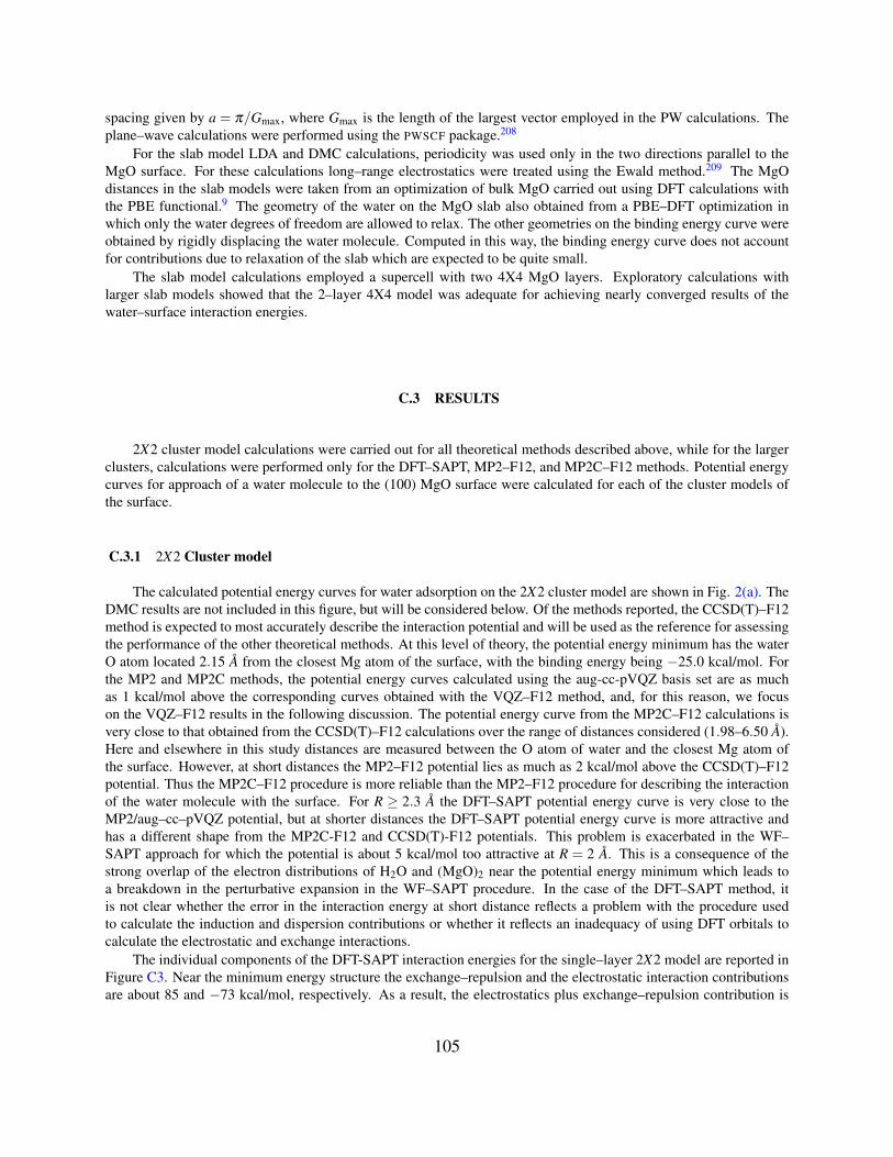
spacing given by a = π/Gmax, where Gmax is the length of the largest vector employed in the PW calculations. Theplane–wave calculations were performed using the PWSCF package.208
For the slab model LDA and DMC calculations, periodicity was used only in the two directions parallel to theMgO surface. For these calculations long–range electrostatics were treated using the Ewald method.209 The MgOdistances in the slab models were taken from an optimization of bulk MgO carried out using DFT calculations withthe PBE functional.9 The geometry of the water on the MgO slab also obtained from a PBE–DFT optimization inwhich only the water degrees of freedom are allowed to relax. The other geometries on the binding energy curve wereobtained by rigidly displacing the water molecule. Computed in this way, the binding energy curve does not accountfor contributions due to relaxation of the slab which are expected to be quite small.
The slab model calculations employed a supercell with two 4X4 MgO layers. Exploratory calculations withlarger slab models showed that the 2–layer 4X4 model was adequate for achieving nearly converged results of thewater–surface interaction energies.
C.3 RESULTS
2X2 cluster model calculations were carried out for all theoretical methods described above, while for the largerclusters, calculations were performed only for the DFT–SAPT, MP2–F12, and MP2C–F12 methods. Potential energycurves for approach of a water molecule to the (100) MgO surface were calculated for each of the cluster models ofthe surface.
C.3.1 2X2 Cluster model
The calculated potential energy curves for water adsorption on the 2X2 cluster model are shown in Fig. 2(a). TheDMC results are not included in this figure, but will be considered below. Of the methods reported, the CCSD(T)–F12method is expected to most accurately describe the interaction potential and will be used as the reference for assessingthe performance of the other theoretical methods. At this level of theory, the potential energy minimum has the waterO atom located 2.15 A from the closest Mg atom of the surface, with the binding energy being −25.0 kcal/mol. Forthe MP2 and MP2C methods, the potential energy curves calculated using the aug-cc-pVQZ basis set are as muchas 1 kcal/mol above the corresponding curves obtained with the VQZ–F12 method, and, for this reason, we focuson the VQZ–F12 results in the following discussion. The potential energy curve from the MP2C–F12 calculations isvery close to that obtained from the CCSD(T)–F12 calculations over the range of distances considered (1.98–6.50 A).Here and elsewhere in this study distances are measured between the O atom of water and the closest Mg atom ofthe surface. However, at short distances the MP2–F12 potential lies as much as 2 kcal/mol above the CCSD(T)–F12potential. Thus the MP2C–F12 procedure is more reliable than the MP2–F12 procedure for describing the interactionof the water molecule with the surface. For R ≥ 2.3 A the DFT–SAPT potential energy curve is very close to theMP2/aug–cc–pVQZ potential, but at shorter distances the DFT–SAPT potential energy curve is more attractive andhas a different shape from the MP2C-F12 and CCSD(T)-F12 potentials. This problem is exacerbated in the WF–SAPT approach for which the potential is about 5 kcal/mol too attractive at R = 2 A. This is a consequence of thestrong overlap of the electron distributions of H2O and (MgO)2 near the potential energy minimum which leads toa breakdown in the perturbative expansion in the WF–SAPT procedure. In the case of the DFT–SAPT method, itis not clear whether the error in the interaction energy at short distance reflects a problem with the procedure usedto calculate the induction and dispersion contributions or whether it reflects an inadequacy of using DFT orbitals tocalculate the electrostatic and exchange interactions.
The individual components of the DFT-SAPT interaction energies for the single–layer 2X2 model are reported inFigure C3. Near the minimum energy structure the exchange–repulsion and the electrostatic interaction contributionsare about 85 and −73 kcal/mol, respectively. As a result, the electrostatics plus exchange–repulsion contribution is
105
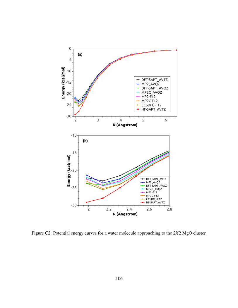
En
erg
y (k
cal/
mo
l)
-30
-25
-20
-15
-10
-5
0
R (Angstrom)2 3 4 5 6
DFT-SAPT_AVTZMP2_AVQZDFT-SAPT_AVQZMP2C_AVQZMP2-F12MP2C-F12CCSD(T)-F12HF-SAPT_AVTZ
(a)
En
erg
y (k
cal/
mo
l)
-30
-25
-20
-15
-10
R (Angstrom)2 2.2 2.4 2.6 2.8
DFT-SAPT_AVTZMP2_AVQZDFT-SAPT_AVQZMP2C_AVQZMP2-F12MP2C-F12CCSD(T)-F12HF-SAPT_AVTZ
(b)
Figure C2: Potential energy curves for a water molecule approaching to the 2X2 MgO cluster.
106
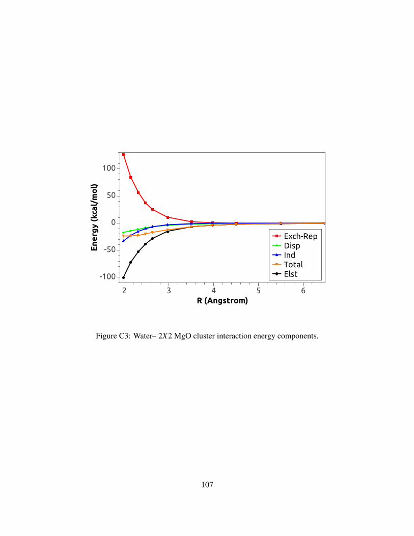
En
erg
y (k
cal/
mo
l)
-100
-50
0
50
100
R (Angstrom)2 3 4 5 6
Exch-RepDispIndTotalElst
Figure C3: Water– 2X2 MgO cluster interaction energy components.
107
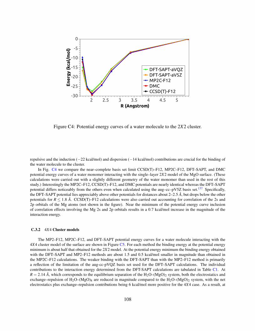
Ene
rgy
(kca
l/m
ol)
-30
-25
-20
-15
-10
-5
0
R (Angstrom)2 2.5 3 3.5 4 4.5 5
DFT-SAPT-aVQZDFT-SAPT-aV5ZMP2C-F12DMCCCSD(T)-F12
Figure C4: Potential energy curves of a water molecule to the 2X2 cluster.
repulsive and the induction (−22 kcal/mol) and dispersion (−14 kcal/mol) contributions are crucial for the binding ofthe water molecule to the cluster.
In Fig. C4 we compare the near–complete basis set limit CCSD(T)–F12, MP2C–F12, DFT–SAPT, and DMCpotential energy curves of a water monomer interacting with the single–layer 2X2 model of the MgO surface. (Thesecalculations were carried out with a slightly different geometry of the water monomer than used in the rest of thisstudy.) Interestingly the MP2C–F12, CCSD(T)–F12, and DMC potentials are nearly identical whereas the DFT–SAPTpotential differs noticeably from the others even when calculated using the aug–cc–pV5Z basis set.137 Specifically,the DFT–SAPT potential lies appreciably above other potentials for distances about 2–2.5 A, but drops below the otherpotentials for R ≤ 1.8 A. CCSD(T)–F12 calculations were also carried out accounting for correlation of the 2s and2p orbitals of the Mg atoms (not shown in the figure). Near the minimum of the potential energy curve inclusionof correlation effects involving the Mg 2s and 2p orbitals results in a 0.7 kcal/mol increase in the magnitude of theinteraction energy.
C.3.2 4X4 Cluster models
The MP2–F12, MP2C–F12, and DFT–SAPT potential energy curves for a water molecule interacting with the4X4 cluster model of the surface are shown in Figure C5. For each method the binding energy at the potential energyminimum is about half that obtained for the 2X2 model. At the potential energy minimum the binding energy obtainedwith the DFT–SAPT and MP2–F12 methods are about 1.5 and 0.5 kcal/mol smaller in magnitude than obtained inthe MP2C–F12 calculations. The weaker binding with the DFT–SAPT than with the MP2–F12 method is primarilya reflection of the limitation of the aug-cc-pVQZ basis set used for the DFT–SAPT calculations. The individualcontributions to the interaction energy determined from the DFT-SAPT calculations are tabulated in Table C1. AtR = 2.14 A, which corresponds to the equilibrium separation of the H2O–(MgO)2 system, both the electrostatics andexchange–repulsion of H2O–(MgO)8 are reduced in magnitude compared to the H2O–(MgO)2 system, with the netelectrostatics plus exchange–repulsion contributions being 6 kcal/mol more positive for the 4X4 case. As a result, at
108
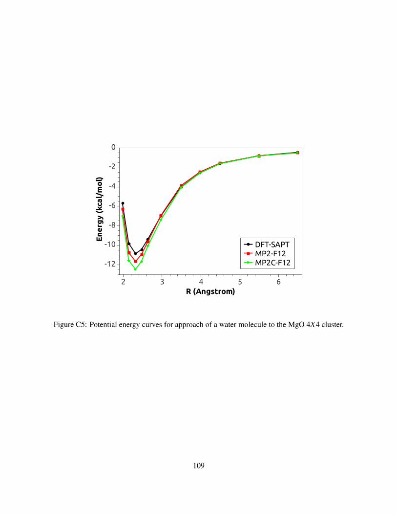
En
erg
y (k
cal/
mo
l)
-12
-10
-8
-6
-4
-2
0
R (Angstrom)2 3 4 5 6
DFT-SAPTMP2-F12MP2C-F12
Figure C5: Potential energy curves for approach of a water molecule to the MgO 4X4 cluster.
109
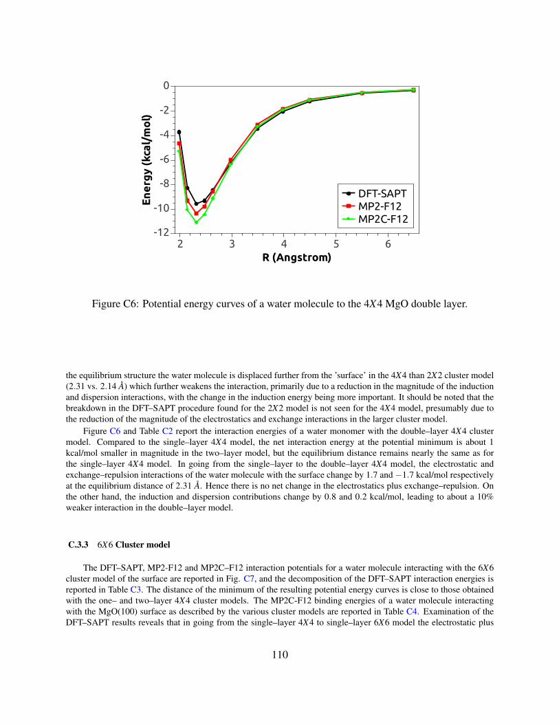
En
erg
y (k
cal/
mo
l)
-12
-10
-8
-6
-4
-2
0
R (Angstrom)2 3 4 5 6
DFT-SAPTMP2-F12MP2C-F12
Figure C6: Potential energy curves of a water molecule to the 4X4 MgO double layer.
the equilibrium structure the water molecule is displaced further from the ’surface’ in the 4X4 than 2X2 cluster model(2.31 vs. 2.14 A) which further weakens the interaction, primarily due to a reduction in the magnitude of the inductionand dispersion interactions, with the change in the induction energy being more important. It should be noted that thebreakdown in the DFT–SAPT procedure found for the 2X2 model is not seen for the 4X4 model, presumably due tothe reduction of the magnitude of the electrostatics and exchange interactions in the larger cluster model.
Figure C6 and Table C2 report the interaction energies of a water monomer with the double–layer 4X4 clustermodel. Compared to the single–layer 4X4 model, the net interaction energy at the potential minimum is about 1kcal/mol smaller in magnitude in the two–layer model, but the equilibrium distance remains nearly the same as forthe single–layer 4X4 model. In going from the single–layer to the double–layer 4X4 model, the electrostatic andexchange–repulsion interactions of the water molecule with the surface change by 1.7 and −1.7 kcal/mol respectivelyat the equilibrium distance of 2.31 A. Hence there is no net change in the electrostatics plus exchange–repulsion. Onthe other hand, the induction and dispersion contributions change by 0.8 and 0.2 kcal/mol, leading to about a 10%weaker interaction in the double–layer model.
C.3.3 6X6 Cluster model
The DFT–SAPT, MP2-F12 and MP2C–F12 interaction potentials for a water molecule interacting with the 6X6cluster model of the surface are reported in Fig. C7, and the decomposition of the DFT–SAPT interaction energies isreported in Table C3. The distance of the minimum of the resulting potential energy curves is close to those obtainedwith the one– and two–layer 4X4 cluster models. The MP2C-F12 binding energies of a water molecule interactingwith the MgO(100) surface as described by the various cluster models are reported in Table C4. Examination of theDFT–SAPT results reveals that in going from the single–layer 4X4 to single–layer 6X6 model the electrostatic plus
110
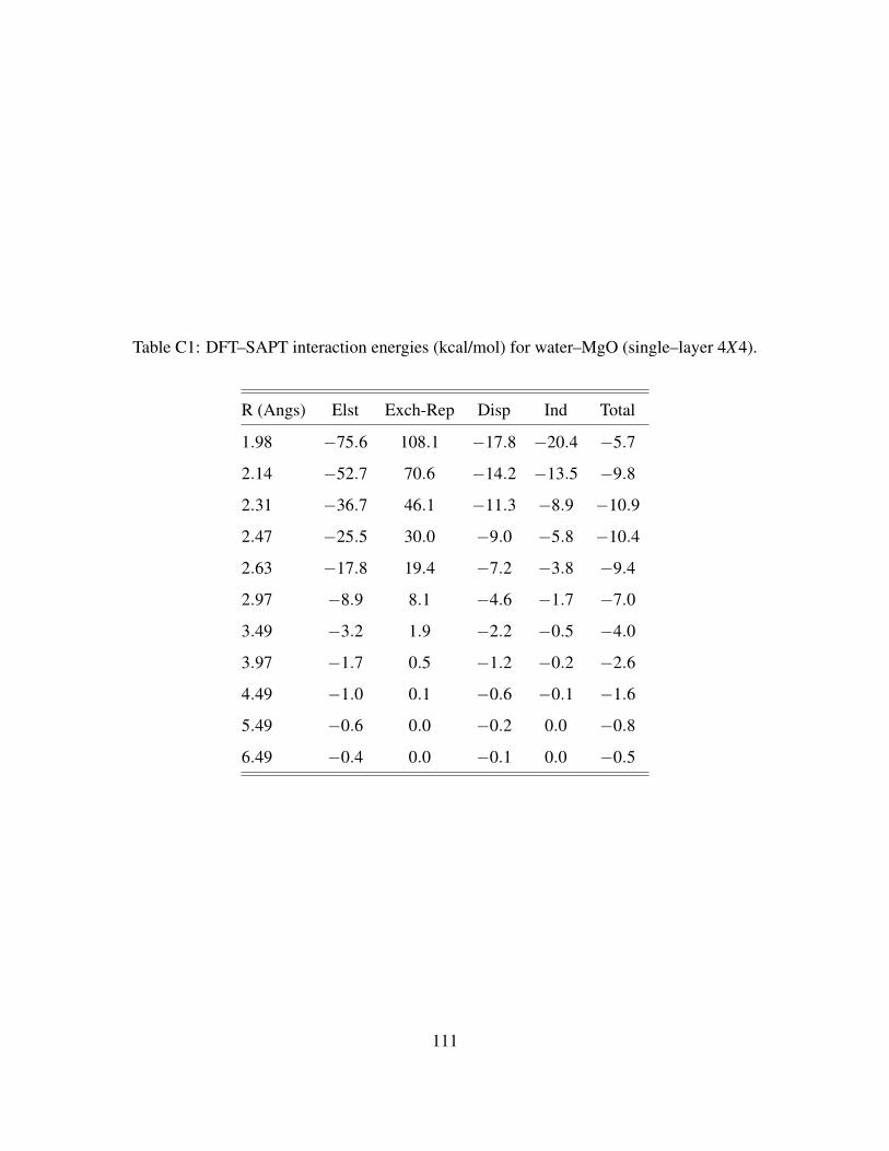
Table C1: DFT–SAPT interaction energies (kcal/mol) for water–MgO (single–layer 4X4).
R (Angs) Elst Exch-Rep Disp Ind Total
1.98 −75.6 108.1 −17.8 −20.4 −5.7
2.14 −52.7 70.6 −14.2 −13.5 −9.8
2.31 −36.7 46.1 −11.3 −8.9 −10.9
2.47 −25.5 30.0 −9.0 −5.8 −10.4
2.63 −17.8 19.4 −7.2 −3.8 −9.4
2.97 −8.9 8.1 −4.6 −1.7 −7.0
3.49 −3.2 1.9 −2.2 −0.5 −4.0
3.97 −1.7 0.5 −1.2 −0.2 −2.6
4.49 −1.0 0.1 −0.6 −0.1 −1.6
5.49 −0.6 0.0 −0.2 0.0 −0.8
6.49 −0.4 0.0 −0.1 0.0 −0.5
111
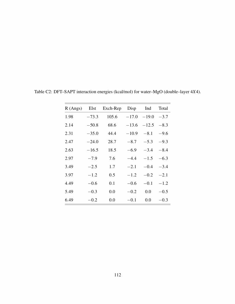
Table C2: DFT–SAPT interaction energies (kcal/mol) for water–MgO (double–layer 4X4).
R (Angs) Elst Exch-Rep Disp Ind Total
1.98 −73.3 105.6 −17.0 −19.0 −3.7
2.14 −50.8 68.6 −13.6 −12.5 −8.3
2.31 −35.0 44.4 −10.9 −8.1 −9.6
2.47 −24.0 28.7 −8.7 −5.3 −9.3
2.63 −16.5 18.5 −6.9 −3.4 −8.4
2.97 −7.9 7.6 −4.4 −1.5 −6.3
3.49 −2.5 1.7 −2.1 −0.4 −3.4
3.97 −1.2 0.5 −1.2 −0.2 −2.1
4.49 −0.6 0.1 −0.6 −0.1 −1.2
5.49 −0.3 0.0 −0.2 0.0 −0.5
6.49 −0.2 0.0 −0.1 0.0 −0.3
112
exchange contribution to the interaction energy changes by only -0.3 kcal/mol, whereas the induction plus dispersioncontribution decreases by 1.0 kcal/mol in magnitude. Table C4 also includes MP2C–F12 results for the double–layerand triple–layer 2X2 models of the surface. From these results it is seen that adsorption energies essentially convergedat the two layers. The convergence of the adsorption energy along the 2X2, 4X4, and 6X6 sequence of single–layercluster models is shown in Fig. C8. Combining the results (at the minima of the potential energy scans) of the single–layer, and double–layer 4X4 models and the single–layer 6X6 model, we estimate the binding energy of a watermolecule for a double–layer 6X6 cluster model to be about −10.6 kcal/mol, which is in reasonable agreement withthe −11.1 kcal/mol DMC result for a water molecule interacting with a 2–layer model of the MgO(100) surface. Acomparison of the potential energy curve estimated for the double–layer 6X6 model using MP2C–F12 energies andfrom the DMC calculations for the 2–layer slab with periodic boundary conditions is presented in Fig. C9. Overallthe agreement between the two potential energy curves is good, with the small discrepency near the potential energyminimum probably reflecting a limitation of the strategy used to estimate the 2–layer 6X6 cluster model results andalso not including the core correlation effects for the Mg atoms.
We note that the temperature programmed desorption measurements of Ref. 5, which gave a value of 15 kcal/molenergy for desorbing from the Mg (100) surface at low coverages, probably detected water molecules that were H–bonded to OH groups on the surface, thereby, enhancing their binding energies.195
C.3.4 GDMA calculations
The electrostatic interaction energy from the DFT–SAPT calculations includes the effects of charge–penetration.In order to estimate the charge–penetration contribution to the electrostatic energy, we calculated atomic charges,dipoles, and quadrupoles using Stone’s generalized distributed moment analysis (GDMA)116 of the MP2/cc-pVDZ136
densities for the (MgO)n cluster models.(The MP2 calculations were performed using Gaussian 03.117) The resultingmoments are summarized in Table C5. This analysis shows that the charge on the interior Mg and O atoms has nosimple trend in the different cluster models. The magnitude of the dipole moment on the central atoms decreasesalong the sequence of models and it becomes zero for the single–layer 6X6 cluster model. The corresponding dipoleson the O atoms are 0.05, 0.03, and 0.26 au. (The absolute values of the dipoles are reported.) The changes in thequadrupole moments with cluster model are more striking. For example, for the central Mg atoms, the value of theQ20 component of the quadrupole is −0.39, −0.07, −0.02, and −0.05 au for the single–layer 2X2, single–layer 4X4,double–layer 4X4, and single–layer 6X6 cluster models, respectively. The corresponding results for the central Oatoms are −0.89, −1.48, −0.74, and −1.40 au. The same trend for the quadrupole moments is also observed ingoing from the central atoms of the 6X6 to the edge atoms. Using the moments from the GDMA analyses of H2Oand the (MgO)n cluster models we calculated the electrostatic interaction energies, with the results being tabulatedin Table C6. The resulting interaction energies are 32.3, 22.1, 22.3 and 22.5 kcal/mol smaller in magnitude thanthe DFT–SAPT electrostatic interaction energies for the single–layer 2X2, single–layer 4X4, double–layer 4X4, andsingle–layer 6X6 cluster models, respectively. These differences can be taken as estimates of the charge–penetrationcontributions to the electrostatic interaction energies. The greater charge–penetration contribution in the 2X2 modelarises in part from the shorter separation of the water molecule from the surface in this case. Calculations using a 2X2cluster model with GDMA moments from the interior 2X2 sub–cluster in the 4X4 cluster model actually gives evenstronger binding of the water molecule to the cluster than obtained with the original 2X2 model. Thus the main factorcausing the weakening of the electrostatic interaction between the water molecule and the surface as one goes from the2X2 to the 4X4 cluster model is the unfavorable electrostatic interaction with the non–central Mg and O atoms ratherthan changes of the charge distribution of the atoms in the central 2X2 region caused by the presence of surroundingions.
113

En
erg
y (k
cal/
mo
l)
-12
-10
-8
-6
-4
-2
0
R (Angstrom)2 3 4 5 6
DFT-SAPTMP2-F12MP2C-F12
Figure C7: Potential energy curves for approach of a water molecule to the MgO 6X6 cluster.
114

Table C3: DFT–SAPT interaction energies (kcal/mol) for water–MgO (single–layer 6X6).
R (Angs) Elst Exch-Rep Disp Ind Total
1.98 −75.3 107.0 −16.3 −19.9 −4.43
2.14 −52.3 69.8 −13.1 −13.2 −8.86
2.25 −40.4 51.6 −11.2 −9.9 −9.88
2.28 −38.6 49.0 −10.9 −9.4 −9.96
2.31 −36.2 45.3 −10.5 −8.7 −10.01
2.47 −25.0 29.4 −8.4 −5.7 −9.66
2.63 −17.3 19.0 −6.7 −3.7 −8.68
2.97 −8.4 7.9 −4.3 −1.6 −6.35
3.49 −2.8 1.8 −2.1 −0.4 −3.48
3.97 −1.3 0.5 −1.2 −0.2 −2.15
4.49 −0.7 0.1 −0.6 −0.1 −1.29
5.49 −0.4 0.0 −0.2 0.0 −0.66
6.49 −0.3 0.0 −0.1 0.0 −0.43
115
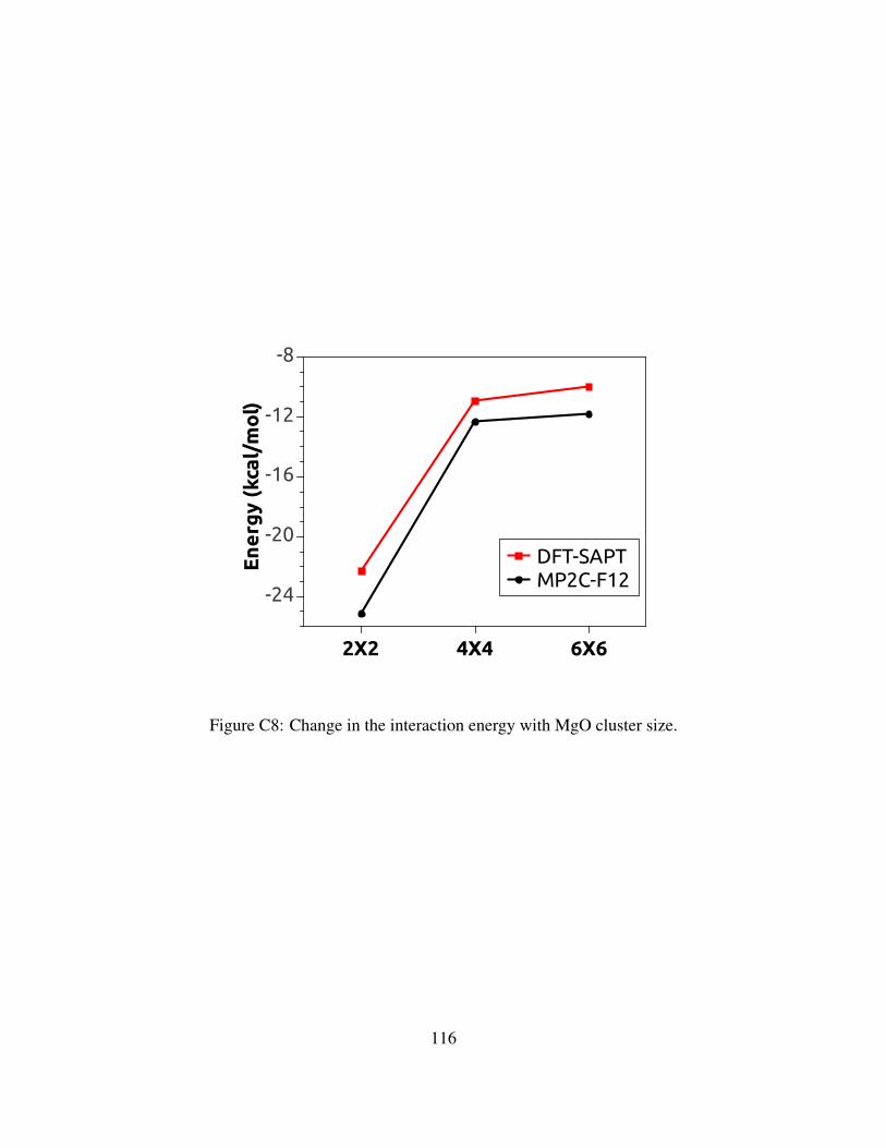
En
erg
y (k
cal/
mo
l)
-24
-20
-16
-12
-8
2X2 4X4 6X6
DFT-SAPTMP2C-F12
Figure C8: Change in the interaction energy with MgO cluster size.
116
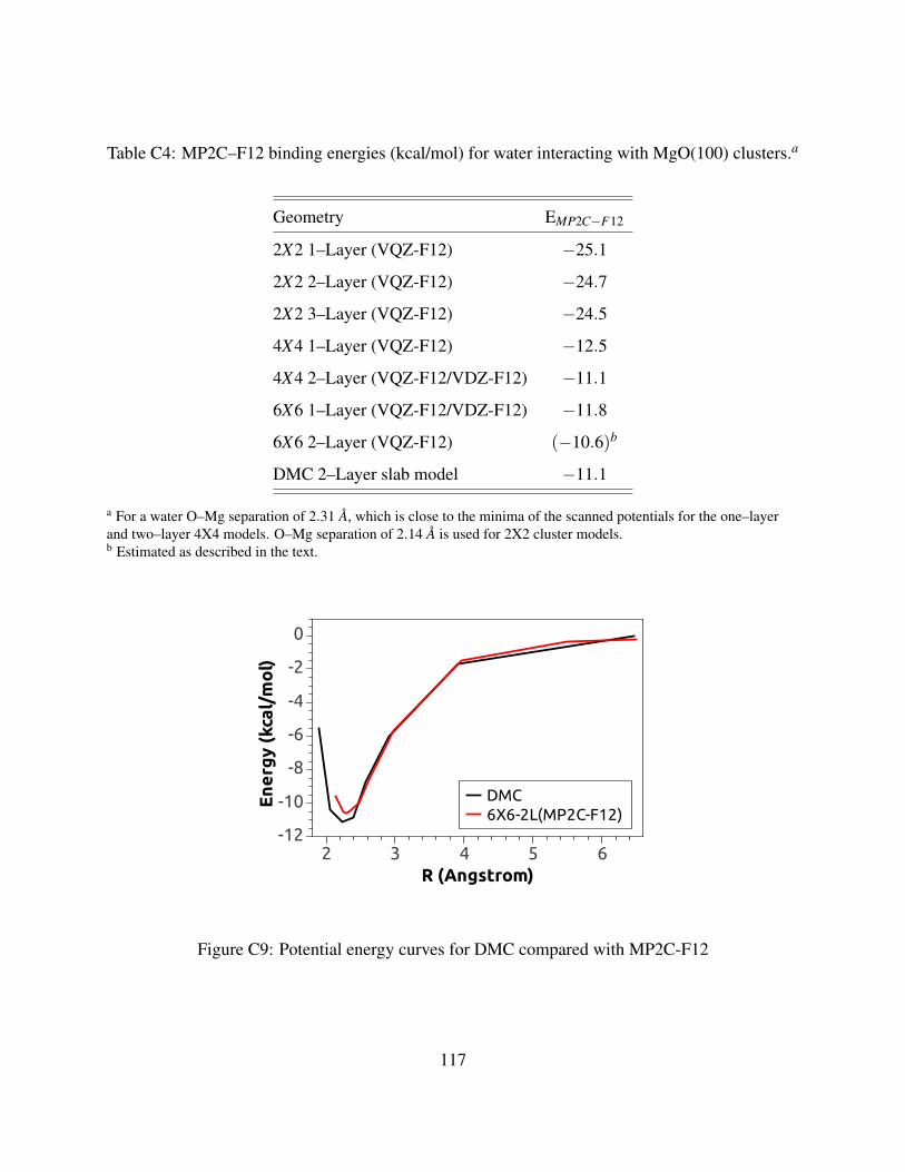
Table C4: MP2C–F12 binding energies (kcal/mol) for water interacting with MgO(100) clusters.a
Geometry EMP2C−F12
2X2 1–Layer (VQZ-F12) −25.1
2X2 2–Layer (VQZ-F12) −24.7
2X2 3–Layer (VQZ-F12) −24.5
4X4 1–Layer (VQZ-F12) −12.5
4X4 2–Layer (VQZ-F12/VDZ-F12) −11.1
6X6 1–Layer (VQZ-F12/VDZ-F12) −11.8
6X6 2–Layer (VQZ-F12) (−10.6)b
DMC 2–Layer slab model −11.1
a For a water O–Mg separation of 2.31 A, which is close to the minima of the scanned potentials for the one–layerand two–layer 4X4 models. O–Mg separation of 2.14 A is used for 2X2 cluster models.b Estimated as described in the text.
En
erg
y (k
cal/
mo
l)
-12
-10
-8
-6
-4
-2
0
R (Angstrom)2 3 4 5 6
DMC6X6-2L(MP2C-F12)
Figure C9: Potential energy curves for DMC compared with MP2C-F12
117
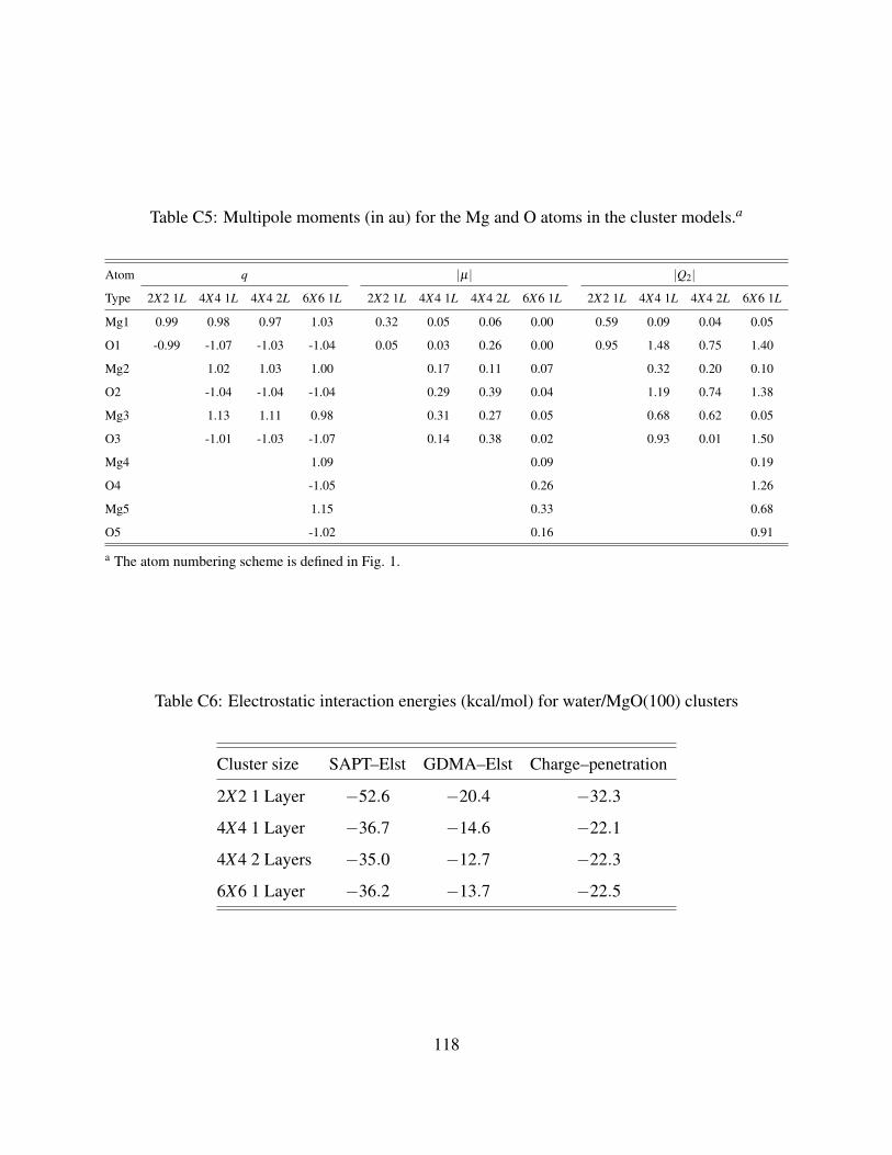
Table C5: Multipole moments (in au) for the Mg and O atoms in the cluster models.a
Atom q |µ| |Q2|
Type 2X2 1L 4X4 1L 4X4 2L 6X6 1L 2X2 1L 4X4 1L 4X4 2L 6X6 1L 2X2 1L 4X4 1L 4X4 2L 6X6 1L
Mg1 0.99 0.98 0.97 1.03 0.32 0.05 0.06 0.00 0.59 0.09 0.04 0.05
O1 -0.99 -1.07 -1.03 -1.04 0.05 0.03 0.26 0.00 0.95 1.48 0.75 1.40
Mg2 1.02 1.03 1.00 0.17 0.11 0.07 0.32 0.20 0.10
O2 -1.04 -1.04 -1.04 0.29 0.39 0.04 1.19 0.74 1.38
Mg3 1.13 1.11 0.98 0.31 0.27 0.05 0.68 0.62 0.05
O3 -1.01 -1.03 -1.07 0.14 0.38 0.02 0.93 0.01 1.50
Mg4 1.09 0.09 0.19
O4 -1.05 0.26 1.26
Mg5 1.15 0.33 0.68
O5 -1.02 0.16 0.91
a The atom numbering scheme is defined in Fig. 1.
Table C6: Electrostatic interaction energies (kcal/mol) for water/MgO(100) clusters
Cluster size SAPT–Elst GDMA–Elst Charge–penetration
2X2 1 Layer −52.6 −20.4 −32.3
4X4 1 Layer −36.7 −14.6 −22.1
4X4 2 Layers −35.0 −12.7 −22.3
6X6 1 Layer −36.2 −13.7 −22.5
118
C.4 CONCLUSIONS
In this study, we have used the MP2, MP2C, and DFT–SAPT methods to calculate the interaction energy of awater molecule with a sequence of cluster models of the MgO(100) surface as well as DMC calculations of a watermonomer interacting with a 2–layer model of the surface. Our calculations show that even a basis set as large as aug-cc-pVQZ does not give well converged interaction energies of a water molecule with cluster models of the surface, andthe F12 approach was adopted to circumvent this problem. Based on the comparison with the results of CCSD(T)–F12 and DMC calculations using the small 2X2 cluster model, it is concluded that the MP2C–F12 approach accuratelydescribes the interaction of a water molecule with the cluster models of the surface. Compared to MP2C–F12, theMP2–F12 method underbinds by about 1 kcal/mol and the DFT–SAPT method underbinds by about 2.5 kcal/mol withabout half the error in this latter case being to limitations in the basis set employed. Going from a single–layer 4X4model to a double–layer 4X4 model, leads to about a 10% reduction of the magnitude of the binding energy. This canbe understood in terms of the unfavorable electrostatic interaction of the water molecule with the second layer Mg andO atoms. Our best estimate of binding energy of a water molecule to the MgO(100) surface obtained from the clustermodel calculations is−10.6 kcal/mol which is in good agreement with the DMC slab model result of−11.1 kcal/mol.At the equilibrium structure of a water molecule on the (100) MgO surface charge–penetration contributes about −22kcal/mol to the interaction energy. As a result, the development of an accurate force field for describing the adsorptionof a water on metal oxide surfaces will require inclusion of explicit charge–penetration terms.
C.5 ACKNOWLEDGEMENTS
This research was carried out with the support of NSF grant CHE–1111235. The SAPT, MP2–F12, MP2C–F12,and CCSD(T)–F12 calculations were carried out on computers in the Pittsburgh University’s Center for Simulationand Modeling. We thank Dr. G. R. Jenness for valuable discussions on SAPT calculations. The DMC calculationswere perfomed on JaguarPF at the Oak Ridge Leadership Computing Facility, located in the National Center for Com-putational Sciences at Oak Ridge National Laboratory, which is supported by the Office of Science of the Departmentof Energy under Contract No. DE–AC05–00OR22725. We are grateful to Dr. Ching-Ming Wei for sharing his Mgpseudopotential.
119
BIBLIOGRAPHY
[1] P. Hohenberg and W. Kohn. Inhomogeneous Electron Gas. Phys. Rev., 136(3B):B864–B871,Nov 1964.
[2] W. Kohn and L. J. Sham. Self-Consistent Equations Including Exchange and CorrelationEffects. Phys. Rev., 140(4A):A1133–A1138, Nov 1965.
[3] Anthony J. Stone. The Theory of Intermolecular Forces. Oxford University Press, Oxford,U. K., 2002 edition, 1996.
[4] I. G. Kaplan. Intermolecular Interactions: Physical Picture, Computational Methods andModel Potentials. Wiley, New York, 2006.
[5] V. A. Parsegian. Van der Waals Forces. A Handbook for Biologists, Chemists, Engineers,and Physicists. Cambridge University Press, Cambridge, 2006.
[6] J. N. Israelachvili. Intermolecular and Surface Forces. Academic, New York, 1985.
[7] Mel Levy. Universal variational functionals of electron densities, first-order density matri-ces, and natural spin-orbitals and solution of the v-representability problem. PNAS, 76:6062,1979.
[8] R. G. Parr and W. Yang. Density-Functional Theory of Atoms and Molecules. OxfordUniversity Press, New York, 1989.
[9] John P. Perdew, Kieron Burke, and Matthias Ernzerhof. Generalized Gradient Approxima-tion Made Simple. Phys. Rev. Lett., 77(18):3865–3868, Oct 1996.
[10] Jose M. Perez-Jorda and A. D. Becke. A density-functional study of van der Waals forces:rare gas diatomics. Chem. Phys. Lett., 233(1-2):134 – 137, 1995.
[11] Sandor Kristyan and Peter Pulay. Can (semi)local density functional theory account for theLondon dispersion forces? Chem. Phys. Lett., 229(3):175 – 180, 1994.
120
[12] O. Anatole von Lilienfeld, Ivano Tavernelli, Ursula Rothlisberger, and Daniel Sebastiani.Optimization of Effective Atom Centered Potentials for London Dispersion Forces in Den-sity Functional Theory. Phys. Rev. Lett., 93(15):153004, Oct 2004.
[13] I-Chun Lin, Maurıcio D. Coutinho-Neto, Camille Felsenheimer, O. Anatole von Lilienfeld,Ivano Tavernelli, and Ursula Rothlisberger. Library of dispersion-corrected atom-centeredpotentials for generalized gradient approximation functionals: Elements H, C, N, O, He, Ne,Ar, and Kr. Phys. Rev. B, 75(20):205131, May 2007.
[14] Pier Luigi Silvestrelli. Van der Waals interactions in density functional theory by combiningthe quantum harmonic oscillator-model with localized Wannier functions. J. Chem. Phys.,139(5):054106, 2013.
[15] Robert A. DiStasio, O. Anatole von Lilienfeld, and Alexandre Tkatchenko. Collectivemany-body van der Waals interactions in molecular systems. Proc. Natl. Acad. Sci.,109(37):14791–14795, 2012.
[16] Andreas Heßelmann. Long-range correlation energies from frequency-dependent weightedexchange-hole dipole polarisabilities. The Journal of Chemical Physics, 136(1):014104,2012.
[17] Andreas Heßelmann. Assessment of a Nonlocal Correction Scheme to Semilocal DensityFunctional Theory Methods. J. Chem. Theory Comput., 9(1):273–283, 2013.
[18] Qin Wu and Weitao Yang. Empirical correction to density functional theory for van derWaals interactions. J. Chem. Phys., 116(2):515–524, 2002.
[19] Lampros Andrinopoulos, Nicholas D. M. Hine, and Arash A. Mostofi. Calculatingdispersion interactions using maximally localized Wannier functions. J. Chem. Phys.,135(15):154105, 2011.
[20] Stefan Grimme. Accurate description of van der waals complexes by density functionaltheory including empirical corrections. J. Comp. Chem., 25(12):1463–1473, 2004.
[21] Stefan Grimme. Semiempirical GGA-type density functional constructed with a long-rangedispersion correction. J. Comp. Chem., 27(15):1787–1799, 2006.
[22] Stefan Grimme, Jens Antony, Stephan Ehrlich, and Helge Krieg. A consistent and accurateab initio parametrization of density functional dispersion correction (DFT-D) for the 94elements H-Pu. J. Chem. Phys., 132(15):154104, 2010.
[23] Erin R. Johnson and Axel D. Becke. A post-Hartree-Fock model of intermolecular interac-tions: Inclusion of higher-order corrections. J. Chem. Phys., 124(17):174104, 2006.
121

[24] Alexandre Tkatchenko and Matthias Scheffler. Accurate Molecular Van Der Waals Interac-tions from Ground-State Electron Density and Free-Atom Reference Data. Phys. Rev. Lett.,102(7):073005, 2009.
[25] Takeshi Sato and Hiromi Nakai. Density functional method including weak interactions:Dispersion coefficients based on the local response approximation. The Journal of ChemicalPhysics, 131(22):224104, 2009.
[26] Yan Zhao and Donald G. Truhlar. The M06 suite of density functionals for main group ther-mochemistry, thermochemical kinetics, noncovalent interactions, excited states, and transi-tion elements: two new functionals and systematic testing of four M06-class functionals and12 other functionals. Theo. Chim. Acta, 120:215–241, 2008.
[27] M. Dion, H. Rydberg, E. Schroder, D. C. Langreth, and B. I. Lundqvist. Van der WaalsDensity Functional for General Geometries. Phys. Rev. Lett., 92(24):246401, Jun 2004.
[28] Kyuho Lee, Eamonn D. Murray, Lingzhu Kong, Bengt I. Lundqvist, and David C. Langreth.Higher-accuracy van der Waals density functional. Phys. Rev. B, 82(8):081101, Aug 2010.
[29] Oleg A. Vydrov and Troy Van Voorhis. Improving the accuracy of the nonlocal van derWaals density functional with minimal empiricism. J. Chem. Phys., 130(10):104105, 2009.
[30] Petr Jurecka, Jiri Cerny, Pavel Hobza, and Dennis R. Salahub. Density functional theoryaugmented with an empirical dispersion term. Interaction energies and geometries of 80noncovalent complexes compared with ab initio quantum mechanics calculations. J. Com-put. Chem., 28(2):555–569, 2007.
[31] Felix O. Kannemann and Axel D. Becke. Van der Waals Interactions in Density-FunctionalTheory: Rare-Gas Diatomics. Journal of Chemical Theory and Computation, 5(4):719–727,April 2009.
[32] J. Hepburn, G. Scoles, and R. Penco. A simple but reliable method for the prediction ofintermolecular potentials. Chemical Physics Letters, 36(4):451 – 456, 1975.
[33] Jeng-Da Chai and Martin Head-Gordon. Long-range corrected hybrid density functionalswith damped atom-atom dispersion corrections. Phys. Chem. Chem. Phys., 10:6615–6620,2008.
[34] Carlo Adamo and Vincenzo Barone. Toward reliable density functional methods withoutadjustable parameters: The PBE0 model. J. Chem. Phys., 110(13):6158–6170, 1999.
[35] Stefan Grimme, Stephan Ehrlich, and Lars Goerigk. Effect of the damping functionin dispersion corrected density functional theory. Journal of Computational Chemistry,32(7):1456–1465, 2011.
122

[36] Lori A. Burns, Alvaro Vazquez Mayagoitia, Bobby G. Sumpter, and C. David Sherrill.Density-functional approaches to noncovalent interactions: A comparison of dispersion cor-rections (DFT-D), exchange-hole dipole moment (XDM) theory, and specialized function-als. The Journal of Chemical Physics, 134(8):084107, 2011.
[37] X. Chu and A. Dalgarno. Linear response time-dependent density functional theory for vander Waals coefficients. The Journal of Chemical Physics, 121(9):4083–4088, 2004.
[38] F. L. Hirshfeld. Bonded-atom fragments for describing molecular charge densities. Theo.Chim. Acta, 44:129–138, 1977.
[39] A. Otero-de-la Roza and Erin R. Johnson. Many-body dispersion interactions from theexchange-hole dipole moment model. The Journal of Chemical Physics, 138(5):054103,2013.
[40] O. Anatole von Lilienfeld and Alexandre Tkatchenko. Two- and three-body interatomicdispersion energy contributions to binding in molecules and solids. The Journal of ChemicalPhysics, 132(23):234109, 2010.
[41] Alexandre Tkatchenko, Robert A. DiStasio, Roberto Car, and Matthias Scheffler. Accu-rate and Efficient Method for Many-Body van der Waals Interactions. Phys. Rev. Lett.,108:236402, Jun 2012.
[42] Tobias Risthaus and Stefan Grimme. Benchmarking of London Dispersion-AccountingDensity Functional Theory Methods on Very Large Molecular Complexes. Journal ofChemical Theory and Computation, 9(3):1580–1591, 2013.
[43] Anthony M. Reilly and Alexandre Tkatchenko. Seamless and Accurate Modeling of OrganicMolecular Materials. The Journal of Physical Chemistry Letters, 4(6):1028–1033, 2013.
[44] Leonard Kleinman and D. M. Bylander. Efficacious Form for Model Pseudopotentials. Phys.Rev. Lett., 48(20):1425–1428, May 1982.
[45] S. Goedecker, M. Teter, and J. Hutter. Separable dual-space Gaussian pseudopotentials.Phys. Rev. B, 54(3):1703–1710, Jul 1996.
[46] Krishnan Raghavachari, Gary W. Trucks, John A. Pople, and Martin Head-Gordon. Afifth-order perturbation comparison of electron correlation theories. Chem. Phys. Lett.,157(6):479 – 483, 1989.
[47] A. D. Becke. Density-functional exchange-energy approximation with correct asymptoticbehavior. Phys. Rev. A, 38(6):3098–3100, Sep 1988.
123
[48] Chengteh Lee, Weitao Yang, and Robert G. Parr. Development of the Colle-Salvetticorrelation-energy formula into a functional of the electron density. Phys. Rev. B, 37(2):785–789, Jan 1988.
[49] John P. Perdew. Density-functional approximation for the correlation energy of the inhomo-geneous electron gas. Phys. Rev. B, 33(12):8822–8824, Jun 1986.
[50] I-Chun Lin and Ursula Rothlisberger. Describing weak interactions of biomolecules withdispersion-corrected density functional theory. Phys. Chem. Chem. Phys., 10:2730–2734,2008.
[51] I-Chun Lin, Ari P. Seitsonen, Mauricio D. Coutinho-Neto, Ivano Tavernelli, and UrsulaRothlisberger. Importance of van der Waals Interactions in Liquid Water. J. Phys. Chem. B,113(4):1127–1131, 2009.
[52] Radhakrishnan Balu, Edward F. C. Byrd, and Betsy M. Rice. Assessment of DispersionCorrected Atom Centered Pseudopotentials: Application to Energetic Molecular Crystals.J. Phys. Chem. B, 115(5):803–810, 2011.
[53] G. Jenness, O. Karalti, and K. D. Jordan. Benchmark calculations of water-acene interactionenergies: Extrapolation to the water-graphene limit and assessment of dispersion-correctedDFT methods. Phys. Chem. Chem. Phys., 12:6375–6381, 2010.
[54] Glen R. Jenness, Ozan Karalti, W. A. Al-Saidi, and Kenneth D. Jordan. Evaluation ofTheoretical Approaches for Describing the Interaction of Water with Linear Acenes. J.Phys. Chem. A, 115(23):5955–5964, 2011.
[55] Ozan Karalti, Glen R. Jenness, Wissam Al-Saidi, and Kenneth D. Jordan. Is the DCACPMethod Primarily Correcting for Dispersion? unpublished results.
[56] Ivano Tavernelli, I-Chun Lin, and Ursula Rothlisberger. Multicenter-type corrections tostandard DFT exchange and correlation functionals. Phys. Rev. B, 79(4):045106, 2009.
[57] T. Thonhauser, Valentino R. Cooper, Shen Li, Aaron Puzder, Per Hyldgaard, and David C.Langreth. Van der Waals density functional: Self-consistent potential and the nature of thevan der Waals bond. Phys. Rev. B, 76(12):125112, September 2007.
[58] Oleg A. Vydrov and Troy Van Voorhis. Dispersion interactions from a local polarizabilitymodel. Phys. Rev. A, 81(6):062708, June 2010.
[59] John F. Dobson and Tim Gould. Calculation of dispersion energies. Journal of Physics:Condensed Matter, 24(7):073201, 2012.
[60] Y. Zhang and W. Yang. Comment on Generalized Gradient Approximation Made Simple.Phys. Rev. Lett., 80:890, 1998.
124
[61] Aaron Puzder, Maxime Dion, and David C. Langreth. Binding energies in benzenedimers: Nonlocal density functional calculations. The Journal of Chemical Physics,124(16):164105, 2006.
[62] John P. Perdew and Wang Yue. Accurate and simple density functional for the electronicexchange energy: Generalized gradient approximation. Phys. Rev. B, 33:8800–8802, Jun1986.
[63] Guillermo Roman-Perez and Jose M. Soler. Efficient Implementation of a van der WaalsDensity Functional: Application to Double-Wall Carbon Nanotubes. Phys. Rev. Lett.,103(9):096102, Aug 2009.
[64] Pier Luigi Silvestrelli, Karima Benyahia, Sonja Grubisic, Francesco Ancilotto, and FlavioToigo. Van der Waals interactions at surfaces by density functional theory using Wannierfunctions. J. Chem. Phys., 130(7):074702, 2009.
[65] Filipp Furche. Molecular tests of the random phase approximation to the exchange-correlation energy functional. Phys. Rev. B, 64:195120, Oct 2001.
[66] Filipp Furche and Troy Van Voorhis. Fluctuation-dissipation theorem density-functionaltheory. The Journal of Chemical Physics, 122(16):164106, 2005.
[67] Judith Harl and Georg Kresse. Cohesive energy curves for noble gas solids calculated byadiabatic connection fluctuation-dissipation theory. Phys. Rev. B, 77:045136, Jan 2008.
[68] Gustavo E. Scuseria, Thomas M. Henderson, and Danny C. Sorensen. The ground statecorrelation energy of the random phase approximation from a ring coupled cluster doublesapproach. The Journal of Chemical Physics, 129(23):231101, 2008.
[69] Judith Harl and Georg Kresse. Accurate Bulk Properties from Approximate Many-BodyTechniques. Phys. Rev. Lett., 103(5):056401, July 2009.
[70] Xinguo Ren, Patrick Rinke, and Matthias Scheffler. Exploring the random phase approxi-mation: Application to CO adsorbed on Cu(111). Phys. Rev. B, 80(4):045402, July 2009.
[71] Wim Klopper, Andrew M. Teale, Sonia Coriani, Thomas Bondo Pedersen, and Trygve Hel-gaker. Spin flipping in ring-coupled-cluster-doubles theory. Chemical Physics Letters,510(13):147 – 153, 2011.
[72] Janos G. Angyan, Ru-Fen Liu, Julien Toulouse, and Georg Jansen. Correlation Energy Ex-pressions from the Adiabatic-Connection Fluctuation-Dissipation Theorem Approach. Jour-nal of Chemical Theory and Computation, 7(10):3116–3130, 2011.
125

[73] Andreas Heßelmann and Andreas Gorling. Correct Description of the Bond DissociationLimit without Breaking Spin Symmetry by a Random-Phase-Approximation CorrelationFunctional. Phys. Rev. Lett., 106:093001, Feb 2011.
[74] David Bohm and David Pines. A Collective Description of Electron Interactions: III.Coulomb Interactions in a Degenerate Electron Gas. Phys. Rev., 92(3):609–625, Novem-ber 1953.
[75] D.C. Langreth and J.P. Perdew. The exchange-correlation energy of a metallic surface. SolidState Communications, 17(11):1425 – 1429, 1975.
[76] D. C. Langreth and J. P. Perdew. The Exchange-Correlation Energy of a Metallic Surface:Wavevector Analysis. Phys. Rev. B, 15:2884, 1977.
[77] Janos G. Angyan, Iann C. Gerber, Andreas Savin, and Julien Toulouse. van der Waalsforces in density functional theory: Perturbational long-range electron-interaction correc-tions. Phys. Rev. A, 72:012510, Jul 2005.
[78] Julien Toulouse, Fran cois Colonna, and Andreas Savin. Long-range-short-range separationof the electron-electron interaction in density-functional theory. Phys. Rev. A, 70:062505,Dec 2004.
[79] Alexander I. Kolesnikov, Jean-Marc Zanotti, Chun-Keung Loong, Pappannan Thiyagarajan,Alexander P. Moravsky, Raouf O. Loutfy, and Christian J. Burnham. Anomalously SoftDynamics of Water in a Nanotube: A Revelation of Nanoscale Confinement. Phys. Rev.Lett., 93(3):035503, Jul 2004.
[80] David Feller and Kenneth D. Jordan. Estimating the Strength of the Water/Single-LayerGraphite Interaction. J. Phys. Chem. A, 104:9971–9975, 2000.
[81] Tim O. Wehling, Alexander I. Lichtenstein, and Mikhail I. Katsnelson. First-principlesstudies of water adsorption on graphene: The role of the substrate. App. Phys. Lett.,93(20):202110, 2008.
[82] O. Leenaerts, B. Partoens, and F. M. Peeters. Adsorption of H2O, NH3, CO, NO2, and NOon graphene: A first-principles study. Phys. Rev. B, 77(12):125416, 2008.
[83] Miroslav Rubes, Petr Nachtigall, Jirı Vondrasek, and Ota Bludsky. Structure and Stabilityof the Water-Graphite Complexes. J. Phys. Chem. C, 113(19):8412–8419, 2009.
[84] Glen R. Jenness and Kenneth D. Jordan. DF-DFT-SAPT Investigation of the Interactionof a Water Molecule to Coronene and Dodecabenzocoronene: Implications for the Water-Graphite Interaction. J. Phys. Chem. C, 113(23):10242–10248, 2009.
126

[85] Fangfang Wang, Glen Jenness, Wissam A. Al-Saidi, and Kenneth D. Jordan. Assessmentof the Performance of Common Density Functional Methods for Describing the InteractionEnergies of (H2O)6 Clusters. J. Chem. Phys., 132:134303, 2010.
[86] S. J. A. van Gisbergen, P. R. T. Schipper, O. V. Gritsenko, E. J. Baerends, J. G. Snijders,B. Champagne, and B. Kirtman. Electric Field Dependence of the Exchange-CorrelationPotential in Molecular Chains. Phys. Rev. Lett., 83(4):694–697, Jul 1999.
[87] Slawomir M. Cybulski and Marion L. Lytle. The origin of deficiency of the supermoleculesecond-order Moller-Plesset approach for evaluating interaction energies. J. Chem. Phys.,127(14):141102, 2007.
[88] Petr Jurecka, Jirı Sponer, Jirı Cerny, and Pavel Hobza. Benchmark database of accurate(MP2 and CCSD(T) complete basis set limit) interaction energies of small model complexes,DNA base pairs, and amino acid pairs. Phys. Chem. Chem. Phys., 8:1985–1993, 2006.
[89] Stefan Grimme. Improved second-order Moller–Plesset perturbation theory by sepa-rate scaling of parallel- and antiparallel-spin pair correlation energies. J. Chem. Phys.,118(20):9095–9102, 2003.
[90] Jens Antony and Stefan Grimme. Is Spin-Component Scaled Second-Order Moller–PlessetPerturbation Theory an Appropriate Method for the Study of Noncovalent Interactions inMolecules? J. Phys. Chem. A, 111(22):4862–4868, June 2007.
[91] Alexandre Tkatchenko, Jr. Robert A. DiStasio, Martin Head-Gordon, and Matthias Schef-fler. Dispersion-corrected Moller–Plesset second-order perturbation theory. J. Chem. Phys.,131(9):094106, 2009.
[92] Michal Pitonak and Andreas Heßelmann. J. Chem. Theory Comput., 6:168–178, 2010.
[93] Andreas Hermann and Peter Schwerdtfeger. Complete basis set limit second-order Moller–Plesset calculations for the fcc lattices of neon, argon, krypton, and xenon. J. Chem. Phys.,131(24):244508, 2009.
[94] A. Heßelmann, G. Jansen, and M. Schutz. Density-functional theory-symmetry-adaptedintermolecular perturbation theory with density fitting: A new efficient method to studyintermolecular interaction energies. J. Chem. Phys., 122(1):014103, 2005.
[95] H.-J. Werner, P. J. Knowles, R. Lindh, F. R. Manby, M. Schutz, P. Celani, T. Korona,A. Mitrushenkov, G. Rauhut, T. B. Adler, R. D. Amos, A. Bernhardsson, A. Berning, D. L.Cooper, M. J. O. Deegan, A. J. Dobbyn, F. Eckert, E. Goll, C. Hampel, G. Hetzer, T. Hre-nar, G. Knizia, C. Koppl, Y. Liu, A. W. Lloyd, R. A. Mata, A. J. May, S. J. McNicholas,W. Meyer, M. E. Mura, A. Nicklass, P. Palmieri, K. Pfluger, R. Pitzer, M. Reiher, U. Schu-mann, H. Stoll, A. J. Stone, R. Tarroni, T. Thorsteinsson, M. Wang, and A. Wolf. MOLPRO,version 2010.1, a package of ab initio programs, 2010. see www.molpro.net.
127

[96] Michael W. Schmidt, Kim K. Baldridge, Jerry A. Boatz, Steven T. Elbert, Mark S. Gordon,Jan H. Jensen, Shiro Koseki, Nikita Matsunaga, Kiet A. Nguyen, Shujun Su, Theresa L.Windus, Michel Dupuis, and John A. Montgomery Jr. General atomic and molecular elec-tronic structure system. J. Comp. Chem., 14:1347–1363, 1993.
[97] CPMD V3.13 Copyright IBM Corp 1990-2008, Copyright MPI fuer FestkoerperforschungStuttgart 1997-2001.
[98] Volker Blum, Ralf Gehrke, Felix Hanke, Paula Havu, Ville Havu, Xinguo Ren, KarstenReuter, and Matthias Scheffler. Ab initio molecular simulations with numeric atom-centeredorbitals. Comp. Phys. Comm., 180:2175–2196, 2009.
[99] H. W. King. CRC Handbook of Chemistry and Physics, pages 12.15–12.18. CRC Press, 88edition, 2007.
[100] W. S. Benedict, N. Gailar, and Earle K. Plyler. Rotation-Vibration Spectra of DeuteratedWater Vapor. J. Chem. Phys., 24(6):1139–1165, 1956.
[101] I. Wayan Sudiarta and D. J. Wallace Geldart. Interaction Energy of a Water Molecule with aSingle-Layer Graphitic Surface Modeled by Hydrogen- and Fluorine-Terminated Clusters.J. Phys. Chem. A, 110(35):10501–10506, September 2006.
[102] Abraham Reyes, Lioudmila Fomina, Lev Rumsh, and Serguei Fomine. Are water-aromaticcomplexes always stabilized due to π–H interactions? LMP2 study. Int. J. Quant. Chem.,104:335–341, 2007.
[103] Enrique M. Cabaleiro-Lago, Jorge A. Carrazana-Garcıa, and Jesus Rodrıguez-Otero. Studyof the interaction between water and hydrogen sulfide with polycyclic aromatic hydrocar-bons. J. Chem. Phys., 130(23):234307, 2009.
[104] Estelle M. Huff and Peter Pulay. A potential surface for the interaction between water andcoronene as a model for a hydrophobic surface. Mol. Phys., 107:1197–1207, 2009.
[105] Alston J. Misquitta, Rafal Podeszwa, Bogumil Jeziorski, and Krzysztof Szalewicz. Inter-molecular potentials based on symmetry-adapted perturbation theory with dispersion ener-gies from time-dependent density-functional calculations. J. Chem. Phys., 123(21):214103,2005.
[106] Fabio Della Sala and Andreas Gorling. Efficient localized Hartree–Fock methods as effec-tive exact-exchange Kohn–Sham methods for molecules. J. Chem. Phys., 115(13):5718–5732, 2001.
[107] Andreas Heßelmann and Georg Jansen. The helium dimer potential from a combined den-sity functional theory and symmetry–adapted perturbation theory approach using an exactexchange–correlation potential. Phys. Chem. Chem. Phys., 5:5010–5014, 2003.
128
[108] Adem Tekin and Georg Jansen. How accurate is the density functional theory combinedwith symmetry–adapted perturbation theory approach for CH-π and π-π interactions? Acomparison to supermolecular calculations for the acetylene-benzene dimer. Phys. Chem.Chem. Phys., 9:1680–1687, 2007.
[109] F. Weigend. A fully direct RI-HF algorithm: Implementation, optimised auxiliary basis sets,demonstration of accuracy and efficiency. Phys. Chem. Chem. Phys., 4:4285, 2002.
[110] Florian Weigend, Andreas Kohn, and Christof Hattig. Efficient use of the correlation consis-tent basis sets in resolution of the identity MP2 calculations. J. Chem. Phys., 116(8):3175–3183, 2002.
[111] Roberto Peverati and Kim K. Baldridge. Implementation and Performance of DFT-D withRespect to Basis Set and Functional for Study of Dispersion Interactions in Nanoscale Aro-matic Hydrocarbon. J. Chem. Theory Comp., 4:2030–2048, 2008.
[112] Axel D. Becke. Density-functional thermochemistry. V. Systematic optimization ofexchange-correlation functionals. J. Chem. Phys., 107(20):8554–8560, 1997.
[113] V. Havu, V. Blum, P. Havu, and M. Scheffler. Efficient O(N) integration for all–electronelectronic structure calculation using numeric basis functions. J. Comp. Phys., 228(22):8367– 8379, 2009.
[114] Jon Applequist. Atom charge transfer in molecular polarizabilities: application of the Olson-Sundberg model to aliphatic and aromatic hydrocarbons. J. Phys. Chem., 97(22):6016–6023,June 1993.
[115] Francois Dehez, Jean-Christophe Soetens, Christophe Chipot, Janos G. Angyan, and ClaudeMillot. Determination of Distributed Polarizabilities from a Statistical Analysis of InductionEnergies. J. Phys. Chem. A, 104(6):1293–1303, February 2000.
[116] Athony J. Stone. Distributed Multipole Analysis: Stability for Large Basis Sets. J. Chem.Theory Comp., 1:1128, 2005.
[117] M. J. Frisch, G. W. Trucks, H. B. Schlegel, G. E. Scuseria, M. A. Robb, J. R. Cheeseman,J. A. Montgomery, Jr., T. Vreven, K. N. Kudin, J. C. Burant, J. M. Millam, S. S. Iyen-gar, J. Tomasi, V. Barone, B. Mennucci, M. Cossi, G. Scalmani, N. Rega, G. A. Petersson,H. Nakatsuji, M. Hada, M. Ehara, K. Toyota, R. Fukuda, J. Hasegawa, M. Ishida, T. Naka-jima, Y. Honda, O. Kitao, H. Nakai, M. Klene, X. Li, J. E. Knox, H. P. Hratchian, J. B. Cross,V. Bakken, C. Adamo, J. Jaramillo, R. Gomperts, R. E. Stratmann, O. Yazyev, A. J. Austin,R. Cammi, C. Pomelli, J. W. Ochterski, P. Y. Ayala, K. Morokuma, G. A. Voth, P. Salvador,J. J. Dannenberg, V. G. Zakrzewski, S. Dapprich, A. D. Daniels, M. C. Strain, O. Farkas,D. K. Malick, A. D. Rabuck, K. Raghavachari, J. B. Foresman, J. V. Ortiz, Q. Cui, A. G.
129
Baboul, S. Clifford, J. Cioslowski, B. B. Stefanov, G. Liu, A. Liashenko, P. Piskorz, I. Ko-maromi, R. L. Martin, D. J. Fox, T. Keith, M. A. Al-Laham, C. Y. Peng, A. Nanayakkara,M. Challacombe, P. M. W. Gill, B. Johnson, W. Chen, M. W. Wong, C. Gonzalez, and J. A.Pople. Gaussian 03, Revision C.02. Gaussian, Inc., Wallingford, CT, 2004.
[118] Liem X. Dang and Tsun-Mei Chang. Molecular dynamics study of water clusters, liquid, andliquid–vapor interface of water with many-body potentials. J. Chem. Phys., 106(19):8149–8159, 1997.
[119] D. B. Whitehouse and A. D. Buckingham. Experimental Determination of the AtomicQuadrupole Moment of Graphite. J. Chem. Soc. Faraday Trans., 89:1909–1913, 1993.
[120] Matthew J. Allen, Vincent C. Tung, and Richard B. Kaner. Honeycomb Carbon: A Reviewof Graphene. Chem. Rev., 110(1):132–145, January 2010.
[121] Miroslav Rubes, Jirı Kysilka, Petr Nachtigall, and Ota Bludsky. DFT/CC investigation ofphysical adsorption on a graphite (0001) surface. Phys. Chem. Chem. Phys., 12:6438–6444,2010.
[122] G. Forte, A. Grassi, G. M. Lombardo, G. G. N. Angilella, N. H. March, and R. Pucci.Quantum-chemical modelling of the structural change of water due to its interaction withnanographene. Phys. Chem. Liq., 47:599–606, 2009.
[123] C. S. Lin, R. Q. Zhang, S. T. Lee, M. Elstner, Th. Frauenheim, and L. J. Wan. Simulation ofWater Cluster Assembly on a Graphite Surface. J. Phys. Chem. B, 109(29):14183–14188,July 2005.
[124] D C Langreth, B I Lundqvist, S D Chakarova-Kack, V R Cooper, M Dion, P Hyldgaard,A Kelkkanen, J Kleis, Lingzhu Kong, Shen Li, P G Moses, E Murray, A Puzder, H Rydberg,E Schrder, and T Thonhauser. A density functional for sparse matter. Journal of Physics:Condensed Matter, 21(8):084203, 2009.
[125] Attila Szabo and Neil S. Ostlund. Modern Quantum Chemistry: Introduction to AdvancedElectronic Structure Theory. Dover Publications, Inc., 1996.
[126] Claudia Hampel, Kirk A. Peterson, and Hans-Joachim Werner. A comparison of the ef-ficiency and accuracy of the quadratic configuration interaction (QCISD), coupled cluster(CCSD), and Brueckner coupled cluster (BCCD) methods. Chem. Phys. Lett., 190(1-2):1 –12, 1992.
[127] Miles J. O. Deegan and Peter J. Knowles. Perturbative corrections to account for tripleexcitations in closed and open shell coupled cluster theories. Chem. Phys. Lett., 227(3):321– 326, 1994.
130
[128] Stefan Kurth and John P. Perdew. Density-functional correction of random-phase-approximation correlation with results for jellium surface energies. Phys. Rev. B,59(16):10461–10468, Apr 1999.
[129] Zidan Yan, John P. Perdew, and Stefan Kurth. Density functional for short-range correlation:Accuracy of the random-phase approximation for isoelectronic energy changes. Phys. Rev.B, 61(24):16430–16439, Jun 2000.
[130] X. Ren and V. Blum. Private Communication, 2010.
[131] Miroslav Rubes, Pavel Soldan, Petr Nachtigall, and Ota Bludsky. A Computationally Feasi-ble DFT/CCSD(T) Correction Scheme for the Description of Weakly Interacting Systems.O. Chem. Phys. J., 1:1–11, 2008.
[132] G. Kresse and J. Hafner. Ab initio molecular dynamics for liquid metals. Phys. Rev. B,47(1):558–561, Jan 1993.
[133] G. Kresse and J. Hafner. Ab initio molecular-dynamics simulation of the liquid-metal–amorphous-semiconductor transition in germanium. Phys. Rev. B, 49(20):14251–14269,May 1994.
[134] G. Kresse and J. Furthmller. Efficiency of ab-initio total energy calculations for metals andsemiconductors using a plane-wave basis set. Comput. Mat. Sci., 6:15, 1996.
[135] G. Kresse and J. Furthmuller. Efficient iterative schemes for ab initio total-energy calcula-tions using a plane-wave basis set. Phys. Rev. B, 54(16):11169–11186, Oct 1996.
[136] Thom H. Dunning, Jr. Gaussian basis sets for use in correlated molecular calculations. I.The atoms boron through neon and hydrogen. J. Chem. Phys., 90(2):1007–1023, 1989.
[137] Rick A. Kendall, Thom H. Dunning , Jr., and Robert J. Harrison. Electron affinities ofthe first-row atoms revisited. Systematic basis sets and wave functions. J. Chem. Phys.,96(9):6796–6806, 1992.
[138] Hans-Joachim Werner, Thomas B. Adler, and Frederick R. Manby. General orbital invariantMP2-F12 theory. J. Chem. Phys., 126(16):164102, 2007.
[139] Thomas B. Adler, Gerald Knizia, and Hans-Joachim Werner. A simple and efficientCCSD(T)-F12 approximation. J. Chem. Phys., 127(22):221106, 2007.
[140] Gerald Knizia, Thomas B. Adler, and Hans-Joachim Werner. Simplified CCSD(T)-F12methods: Theory and benchmarks. J. Chem. Phys., 130(5):054104, 2009.
131
[141] Kevin E. Riley, Michal Pitonak, Petr Jurecka, and Pavel Hobza. Stabilization and StructureCalculations for Noncovalent Interactions in Extended Molecular Systems Based on WaveFunction and Density Functional Theories. Chem. Rev., 110:5023–5063, May 2010.
[142] Andreas Heßelmann. Improved supermolecular second order Moller–Plesset intermolecu-lar interaction energies using time-dependent density functional response theory. J. Chem.Phys., 128(14):144112, 2008.
[143] Andreas Heßelmann. Private Communication, 2010.
[144] Kirk A. Peterson, Thomas B. Adler, and Hans-Joachim Werner. Systematically convergentbasis sets for explicitly correlated wavefunctions: The atoms H, He, B–Ne, and Al–Ar. J.Chem. Phys., 128(8):084102, 2008.
[145] John A. Pople, Martin Head-Gordon, and Krishnan Raghavachari. Quadratic configurationinteraction. A general technique for determining electron correlation energies. The Journalof Chemical Physics, 87(10):5968–5975, 1987.
[146] S. F. Boys and F. Bernardi. The calculation of small molecular interactions by the differencesof separate total energies. Some procedures with reduced errors. Mol. Phys., 19:553–566,1970.
[147] Andreas Heßelmann and Georg Jansen. First-order intermolecular interaction energies fromKohn-Sham orbitals. Chem. Phys. Lett., 357(5-6):464 – 470, 2002.
[148] Andreas Heßelmann and Georg Jansen. Intermolecular induction and exchange-inductionenergies from coupled-perturbed Kohn-Sham density functional theory. Chem. Phys. Lett.,362(3-4):319 – 325, 2002.
[149] Andreas Heßelmann and Georg Jansen. Intermolecular dispersion energies from time-dependent density functional theory. Chem. Phys. Lett., 367(5-6):778 – 784, 2003.
[150] S. G. Lias. Ionization Energy Evaluation. NIST Chemistry WebBook, NIST Standard Ref-erence Database No. 69. http://webbook.nist.gov.
[151] T. Koopmans. On the coordination of wave functions and intrinsic values to the singleeletrons of an atom. Physica, 1(1-6):104 – 113, 1934.
[152] Ota Bludsky, Miroslav Rubes, Pavel Soldan, and Petr Nachtigall. Investigation of thebenzene-dimer potential energy surface: DFT/CCSD(T) correction scheme. J. Chem. Phys.,128(11):114102, 2008.
[153] Eamonn D. Murray, Kyuho Lee, and David C. Langreth. Investigation of Exchange En-ergy Density Functional Accuracy for Interacting Molecules. J. Chem. Theory Comput.,5(10):2754–2762, October 2009.
132
[154] Murray Gell-Mann and Keith A. Brueckner. Correlation Energy of an Electron Gas at HighDensity. Phys. Rev., 106:364–368, Apr 1957.
[155] W. J. Hehre, R. Ditchfield, and J. A. Pople. Self-Consistent Molecular Orbital Methods.XII. Further Extensions of Gaussian-Type Basis Sets for Use in Molecular Orbital Studiesof Organic Molecules. J. Chem. Phys., 56(5):2257–2261, 1972.
[156] Michelle M. Francl, William J. Pietro, Warren J. Hehre, J. Stephen Binkley, Mark S. Gordon,Douglas J. DeFrees, and John A. Pople. Self consistent molecular orbital methods. XXIII.A polarization type basis set for second row elements. The Journal of Chemical Physics,77(7):3654–3665, 1982.
[157] M. F. Falcetta and Kenneth D. Jordan. Assignments of the temporary anion states of thechloromethanes. J. Phys. Chem., 94(15):5666–5669, July 1990.
[158] K. N. Houk, Patrick S. Lee, and Maja Nendel. Polyacene and Cyclacene Geometries andElectronic Structures: Bond Equalization, Vanishing Band Gaps, and Triplet Ground StatesContrast with Polyacetylene. J. Org. Chem., 66(16):5517–5521, August 2001.
[159] B. Hajgato, D. Szieberth, P. Geerlings, F. De Proft, and M. S. Deleuze. A benchmarktheoretical study of the electronic ground state and of the singlet-triplet split of benzene andlinear acenes. J. Chem. Phys., 131(22):224321, 2009.
[160] A.J. Stone. Distributed multipole analysis, or how to describe a molecular charge distribu-tion. Chem. Phys. Lett., 83(2):233 – 239, 1981.
[161] S. L. Price and A. J. Stone. A distributed multipole analysis of the charge densities of theazabenzene molecules. Chem. Phys. Lett., 98(5):419 – 423, 1983.
[162] S. L. Price, A. J. Stone, and M. Alderton. Explicit formulae for the electrostatic energy,forces and torques between a pair of molecules of arbitrary symmetry. Mol. Phys., 52:987,1984.
[163] Revati Kumar, Fang-Fang Wang, Glen R. Jenness, and Kenneth D. Jordan. A second gener-ation distributed point polarizable water model. J. Chem. Phys., 132(1):014309, 2010.
[164] R. S. Mulliken. Electronic Population Analysis on LCAO–MO Molecular Wave Functions.I. J. Chem. Phys., 23(10):1833–1840, 1955.
[165] B Jeziorski, R Moszynski, A. Ratkiewicz, S. Rybak, K. Szalewicz, and H. L Williams.In E. Clementi, editor, Method and Techniques in Computational Chemistry: METECC94,volume B, pages 79–129. STEF: Cagliari, Italy, 1993.
133
[166] Bogumil Jeziorski, Robert Moszynski, and Krzysztof Szalewicz. Perturbation Theory Ap-proach to Intermolecular Potential Energy Surfaces of van der Waals Complexes. Chem.Rev., 94(7):1887–1930, November 1994.
[167] Florian Weigend and Reinhart Ahlrichs. Balanced basis sets of split valence, triple zetavalence and quadruple zeta valence quality for H to Rn: Design and assessment of accuracy.Phys. Chem. Chem. Phys., 7:3297–3305, 2005.
[168] Biswajit Santra, Angelos Michaelides, Martin Fuchs, Alexandre Tkatchenko, Claudia Fil-ippi, and Matthias Scheffler. On the accuracy of density-functional theory exchange-correlation functionals for H bonds in small water clusters. II. The water hexamer and vander Waals interactions. J. Chem. Phys., 129(19):194111, 2008.
[169] Erin E. Dahlke, Ryan M. Olson, Hannah R. Leverentz, and Donald G. Truhlar. Assessmentof the Accuracy of Density Functionals for Prediction of Relative Energies and Geometriesof Low-Lying Isomers of Water Hexamers. J. Phys. Chem. A, 112(17):3976–3984, May2008.
[170] Julius T. Su, Xin Xu, and William A. Goddard. Accurate Energies and Structures forLarge Water Clusters Using the X3LYP Hybrid Density Functional. J. Phys. Chem. A,108(47):10518–10526, November 2004.
[171] Andre K. Kelkkanen, Bengt I. Lundqvist, and Jens K. Nørskov. Density functional for vander Waals forces accounts for hydrogen bond in benchmark set of water hexamers. J. Chem.Phys., 131(4):046102, 2009.
[172] Desiree M. Bates and Gregory S. Tschumper. CCSD(T) Complete Basis Set Limit RelativeEnergies for Low-Lying Water Hexamer Structures. J. Phys. Chem. A, 113(15):3555–3559,April 2009.
[173] Sotiris S. Xantheas, Christian J. Burnham, and Robert J. Harrison. Development of transfer-able interaction models for water. II. Accurate energetics of the first few water clusters fromfirst principles. J. Chem. Phys., 116(4):1493–1499, 2002.
[174] Peifeng Su and Hui Li. Energy decomposition analysis of covalent bonds and intermolecularinteractions. J. Chem. Phys., 131(1):014102, 2009.
[175] Luigi Genovese, Alexey Neelov, Stefan Goedecker, Thierry Deutsch, Seyed AlirezaGhasemi, Alexander Willand, Damien Caliste, Oded Zilberberg, Mark Rayson, AndersBergman, and Reinhold Schneider. Daubechies wavelets as a basis set for density func-tional pseudopotential calculations. J. Chem. Phys., 129(1):014109–14, July 2008.
[176] Ingrid Daubechies. Ten Lectures on Wavelets. Society for Industrial and Applied Mathe-matics, 1992.
134

[177] Luigi Genovese, Thierry Deutsch, Alexey Neelov, Stefan Goedecker, and Gregory Beylkin.Efficient solution of Poisson’s equation with free boundary conditions. J. Chem. Phys.,125(7):074105–5, August 2006.
[178] B.M. Adams, W.J. Bohnhoff, K.R. Dalbey, J.P. Eddy, M.S. Eldred, D.M. Gay, K. Haskell,P.D. Hough, and L.P. Swiler. ”DAKOTA, A Multilevel Parallel Object-Oriented Frame-work for Design Optimization, Parameter Estimation, Uncertainty Quantification, and Sen-sitivity Analysis: Version 5.0 User’s Manual,”. Technical report, Sandia Technical ReportSAND2010-2183, 2010.
[179] Mutasem Omar Sinnokrot and C. David Sherrill. Highly Accurate Coupled Cluster Poten-tial Energy Curves for the Benzene Dimer: Sandwich, T-Shaped, and Parallel-DisplacedConfigurations. J. Phys. Chem. A, 108(46):10200–10207, November 2004.
[180] Lucie Grafova, Michal Pitonak, Jan Rezac, and Pavel Hobza. Comparative Study of Se-lected Wave Function and Density Functional Methods for Noncovalent Interaction EnergyCalculations Using the Extended S22 Data Set. J. Chem. Theory Comput., 6(8):2365–2376,2010.
[181] O. Anatole von Lilienfeld. Force correcting atom centred potentials for generalised gra-dient approximated density functional theory: Approaching hybrid functional accuracy forgeometries and harmonic frequencies in small chlorofluorocarbons. Mol. Phys., 111(14-15):2147–2153, 2013.
[182] Ashok Kumar and William J. Meath. Dipole oscillator strength properties and dispersionenergies for acetylene and benzene. Mol. Phys., 75(2):311–324, 1992.
[183] J. Klimes, D. R. Bowler, and A. Michaelides. Chemical accuracy for the van der Waalsdensity functional. J. Phys.: Condens Matter, 22:022201, 2010.
[184] J. Klimes, David R. Bowler, and Angelos Michaelides. Van der Waals density functionalsapplied to solids. Phys. Rev. B, 83:195131, May 2011.
[185] Alston J. Misquitta, Bogumil Jeziorski, and Krzysztof Szalewicz. Dispersion Energy fromDensity-Functional Theory Description of Monomers. Phys. Rev. Lett., 91(3):033201, Jul2003.
[186] Alston J. Misquitta and Krzysztof Szalewicz. Symmetry-adapted perturbation-theory calcu-lations of intermolecular forces employing density-functional description of monomers. J.Chem. Phys., 122(21):214109, 2005.
[187] D. Alfe and M. J. Gillan. Ab initio statistical mechanics of surface adsorption and desorp-tion. I. H2O on MgO (001) at low coverage. J. Chem. Phys., 127(11):114709, 2007.
135
[188] D. Alfe and M. J. Gillan. Ab initio statistical mechanics of surface adsorption and desorp-tion. II. Nuclear quantum effects. J. Chem. Phys., 133(4):044103–9, July 2010.
[189] Jamila Ahdjoudj and Christian Minot. Adsorption of H2O on metal oxides: a periodicab-initio investigation. Surf. Sci., 402-404(0):104 – 109, 1998.
[190] Yan Wang and Thanh N. Truong. Theoretical Study of Adsorption of Water Dimer on thePerfect MgO(100) Surface: Molecular Adsorption versus Dissociative Chemisorption. J.Phys. Chem. B, 108(10):3289–3294, 2004.
[191] Maureen I. McCarthy, Gregory K. Schenter, Carol A. Scamehorn, and John B. Nicholas.Structure and Dynamics of the Water/MgO Interface. J. Phys. Chem., 100(42):16989–16995, 1996.
[192] Michael A. Johnson, Eugene V. Stefanovich, Thanh N. Truong, Jens Gunster, and D. W.Goodman. Dissociation of Water at the MgO(100) Water Interface: Comparison of Theorywith Experiment. J. Phys. Chem. B, 103(17):3391–3398, 1999.
[193] D Ferry, S Picaud, P.N.M Hoang, C Girardet, L Giordano, B Demirdjian, and J Suzanne.Water monolayers on MgO(100): structural investigations by LEED experiments, tensorLEED dynamical analysis and potential calculations. Surf. Sci., 409(1):101 – 116, 1998.
[194] Viacheslav A. Tikhomirov and Karl Jug. MSINDO Study of Water Adsorption on the CleanMgO(100) Surface. J. Phys. Chem. B, 104(32):7619–7622, 2000.
[195] Michael Odelius. Mixed Molecular and Dissociative Water Adsorption on MgO[100]. Phys.Rev. Lett., 82(19):3919–3922, May 1999.
[196] Chr. Moller and M. S. Plesset. Note on an Approximation Treatment for Many-ElectronSystems. Phys. Rev., 46(7):618–622, Oct 1934.
[197] Hans-Joachim Werner, Frederick R. Manby, and Peter J. Knowles. Fast linear scalingsecond-order Moller-Plesset perturbation theory (MP2) using local and density fitting ap-proximations. J. Chem. Phys., 118(18):8149–8160, 2003.
[198] Stanisław Rybak, Bogumił Jeziorski, and Krzysztof Szalewicz. Many-body symmetry-adapted perturbation theory of intermolecular interactions. H2O and HF dimers. J. Chem.Phys., 95(9):6576–6601, 1991.
[199] M. Gruning, O. V. Gritsenko, S. J. A. van Gisbergen, and E. J. Baerends. Shape correctionsto exchange-correlation potentials by gradient-regulated seamless connection of model po-tentials for inner and outer region. J. Chem. Phys., 114(2):652–660, 2001.
136
[200] R J Needs, M D Towler, N D Drummond, and P Lpez Ros. Continuum variational anddiffusion quantum Monte Carlo calculations. J. Phys.: Condensed Matter, 22(2):023201,2010.
[201] M. D. Towler. The quantum Monte Carlo method. phys. stat. sol. (b), 243(11):2573–2598,2006.
[202] C. J. Umrigar, J. Toulouse, C. Filippi, S. Sorella, and R. G. Hennig. Alleviation of theFermion-Sign Problem by Optimization of Many-Body Wave Functions. Phys. Rev. Lett.,98(11):110201, March 2007.
[203] J. Toulouse and C. J. Umrigar. Optimization of quantum Monte Carlo wave functions byenergy minimization. J. Chem. Phys., 126(8):084102–16, February 2007.
[204] L. Mitas, Shirley E. L., and Ceperley D. M. Nonlocal pseudopotentials and diffusion MonteCarlo. J. Chem. Phys., 95(5):3467–3475, 1991.
[205] J. R. Trail and R. J. Needs. Smooth relativistic Hartree–Fock pseudopotentials for H to Baand Lu to Hg. J. Chem. Phys., 122(17):174109, 2005.
[206] Ching-Ming Wei. private communication. private communication.
[207] D. Alfe and M. J. Gillan. Efficient localized basis set for quantum Monte Carlo calculationson condensed matter. Phys. Rev. B, 70(16):161101, October 2004.
[208] S. de Gironcoli S. Baroni, A. Dal Corso and P. Giannozzi. http://www.pwscf.org.
[209] P. P. Ewald. The calculation of optical and electrostatic lattice potentials. Ann. Phys.,369:253, 1921.
137