correction methods jacque shultz b.s., kansas state university
TRANSCRIPT

AUTHENTICATING TURBOCHARGER PERFORMANCE UTILIZING ASME PERFORMANCE TEST CODE
CORRECTION METHODS
by
JACQUE SHULTZ
B.S., Kansas State University, 1998
A THESIS
Submitted in partial fulfillment of the requirements for the degree
MASTER OF SCIENCE
Department of Mechanical and Nuclear Engineering
College of Engineering
KANSAS STATE UNIVERSITY Manhattan, Kansas
2011
Approved by:
Major Professor Dr. Kirby S. Chapman

Copyright
JACQUE SHULTZ
2011

Abstract
Continued regulatory pressure necessitates the use of precisely designed turbochargers to create
the design trapped equivalence ratio within large-bore stationary engines used in the natural gas
transmission industry. The upgraded turbochargers scavenge the exhaust gases from the cylinder,
and create the air manifold pressure and backpressure on the engine necessary to achieve a
specific trapped mass. This combination serves to achieve the emissions reduction required by
regulatory agencies.
Many engine owner/operators request that an upgraded turbocharger be tested and verified prior
to re-installation on engine. Verification of the mechanical integrity and airflow performance
prior to engine installation is necessary to prevent field hardware iterations. Confirming the as-
built turbocharger design specification prior to transporting to the field can decrease downtime
and installation costs. There are however, technical challenges to overcome for comparing test-
cell data to field conditions.
This thesis discusses the required corrections and testing methodology to verify turbocharger
onsite performance from data collected in a precisely designed testing apparatus. As the litmus
test of the testing system, test performance data is corrected to site conditions per the design air
specification. Prior to field installation, the turbocharger is fitted with instrumentation to collect
field operating data to authenticate the turbocharger testing system and correction methods. The
correction method utilized herein is the ASME Performance Test Code 10 (PTC10) for
Compressors and Exhausters version 1997.

- iv -
Table of Contents
Table of Contents........................................................................................................................... iv
List of Figures.............................................................................................................................. viii
List of Tables .................................................................................................................................. x
Acknowledgements........................................................................................................................ xi
Nomenclature................................................................................................................................ xii
CHAPTER 1 : Introduction ............................................................................................................ 1
CHAPTER 2 : Literature Review ................................................................................................... 4
2.1 Turbomachine ....................................................................................................................... 4
2.1.1 How a Turbocharger Works........................................................................................... 4
2.1.2 Centrifugal Compressor ................................................................................................. 6
2.1.3 Turbocharger Use on Engine ......................................................................................... 9
2.2 Motivation to Evaluate Established Performance Correction Models................................ 11
2.3 Volumetric Flow................................................................................................................. 13
2.4 Compression Process .......................................................................................................... 13
2.4.1 Compressible Work ..................................................................................................... 14
2.4.2 Polytropic Compression Process.................................................................................. 16
2.4.3 Isentropic Compression Process .................................................................................. 18
2.4.4 Conclusion of Compressible Work Discussion ........................................................... 21
2.4.5 Compression Power ..................................................................................................... 22
2.4.6 Compressor Polytropic and Isentropic Efficiency ....................................................... 23
2.5 Turbocharger Measurement Locations ............................................................................... 24
2.6 Piping Pressure Losses ....................................................................................................... 26
2.7 Thermodynamic and Fluid Properties ................................................................................ 30

- v -
2.7.1 Mole Fraction and Molecular Weight.......................................................................... 30
2.7.2 Saturated Vapor Pressure of Air .................................................................................. 31
2.7.3 Isobaric Heat Capacity................................................................................................. 33
2.7.4 Ratio of Specific Heats ................................................................................................ 34
2.7.5 Viscosity of Air and Water Vapor ............................................................................... 34
2.7.6 Gas Compressibility..................................................................................................... 35
2.7.7 Total Conditions........................................................................................................... 37
2.8 Dimensional Analysis and Similitude ................................................................................ 38
2.8.1 Units of Measure.......................................................................................................... 40
2.8.2 Fundamental Dimensions............................................................................................. 41
2.8.3 Application of Dimensional Analysis to Centrifugal Compressor .............................. 41
2.8.4 Similitude..................................................................................................................... 46
2.9 Application of Similitude to Centrifugal Compression ...................................................... 47
2.9.1 Flow Coefficient .......................................................................................................... 48
2.9.2 Head Coefficient .......................................................................................................... 50
2.9.3 Power Coefficient ........................................................................................................ 51
2.9.4 Dimensionless Compressor Map ................................................................................. 52
2.9.5 Machine Mach Number ............................................................................................... 52
2.9.6 Machine Reynolds Number ......................................................................................... 54
2.9.7 Reynolds Number Correction for Centrifugal Compressors ....................................... 55
2.9.8 Density Ratio ............................................................................................................... 57
2.10 Concluding Remarks ........................................................................................................ 58
CHAPTER 3 : Test Apparatus...................................................................................................... 60
3.1 Test Cell Design Requirements .......................................................................................... 60

- vi -
3.2 Exhaust Gas Power System ................................................................................................ 61
3.3 Compressor Air System...................................................................................................... 63
3.4 Instrumentation and Performance Data .............................................................................. 63
3.5 Performance Measurement Data......................................................................................... 65
CHAPTER 4 : Turbocharger Specification .................................................................................. 66
4.1 Specified Engine Design Point ........................................................................................... 66
4.2 Compressor Design Point ................................................................................................... 67
4.3 Turbocharger Build Data .................................................................................................... 69
CHAPTER 5 : Test Cell Data ....................................................................................................... 70
5.1 Compressor Test Data......................................................................................................... 70
5.2 Base Compressor Performance Map .................................................................................. 72
5.3 Compressor Discharge Piping Elbow Losses ..................................................................... 73
5.4 Total Tested Gas Condition ................................................................................................ 75
5.5 Dimensionless Coefficients ................................................................................................ 77
5.6 Corrected Compressor Map................................................................................................ 78
5.7 Test Cell Compressor Map at Specified Condition............................................................ 80
CHAPTER 6 : Field Data ............................................................................................................. 82
6.1 Field Installation ................................................................................................................. 82
6.2 Raw Field Data ................................................................................................................... 84
6.3 Compressor Inlet Pressure and Dimensionless Coefficients .............................................. 85
6.4 Correcting to Specified Conditions .................................................................................... 88
CHAPTER 7 : Correlating Test and Field Data ........................................................................... 90
7.1 Dimensionless Coefficient Comparison ............................................................................. 91
7.2 Compressor Map and Field Data Comparison.................................................................... 97

- vii -
7.3 Verifying the Correction Method ....................................................................................... 98
7.3.1 Machine Mach Number Verification ........................................................................... 99
7.3.2 Machine Reynolds Number Correction ..................................................................... 100
7.3.3 Density Ratio ............................................................................................................. 102
7.4 Summary........................................................................................................................... 103
CHAPTER 8 : Conclusions ........................................................................................................ 105
References................................................................................................................................... 107
Appendix A : Saturated Vapor Pressure Methods ...................................................................... 110
Appendix B : Turbocharger Operating Line............................................................................... 111
Appendix C : Overview of Correction Method .......................................................................... 112
Appendix D : Conditions of Ambient Air .................................................................................. 113
Appendix E : Instrument Uncertainty Analysis.......................................................................... 115

- viii -
List of Figures
Figure 2.1: Cutaway of a Turbocharger for a Large-Bore Engine.................................................. 5
Figure 2.2: Comparison Compressor Map of Available Technologies .......................................... 7
Figure 2.3: Variable Speed Compressor Map, Head versus Capacity (Flow) (Ehlers, 1994)........ 8
Figure 2.4: Schematic of Turbocharged Engine (Avallone, 2007)................................................. 9
Figure 2.5: Specific Fuel Consumption and Emissions versus Air to Fuel Ratio ........................ 11
Figure 2.6: Pressure Volume Diagram of Compressible Fluid..................................................... 14
Figure 2.7: Control Volume of Compression Process .................................................................. 15
Figure 2.8: Compressor Performance Measurement Locations (Chapman, 2000)...................... 25
Figure 2.9: Turbine Performance Measurement Locations (Chapman, 2000)............................. 26
Figure 2.10: Moody Chart (Munson, 2002).................................................................................. 28
Figure 2.11: K-Function Saturated Vapor Pressure of Water....................................................... 32
Figure 2.12: Compressibility Chart for Reduced Pressure (Moran, 1995)................................... 36
Figure 2.13: Allowable Machine Mach Number Departure (ASME PTC10-Fig.3.3).................. 53
Figure 2.14: Allowable Machine Reynolds Number Departure (ASME PTC10-Fig.3.5)............ 55
Figure 3.1: Turbocharger Test Cell Layout .................................................................................. 62
Figure 3.2: Turbocharger Test Cell Process and Instrumentation Diagram ................................. 64
Figure 5.1: Compressor Map Prior to Correction ......................................................................... 73
Figure 5.2: Compressor Discharger Header Piping Elbow........................................................... 74
Figure 5.3: Elbow Pressure Loss versus Inlet Volume Flow........................................................ 75
Figure 5.4: Polytropic Head versus Inlet Volume Flow ............................................................... 76
Figure 5.5: Head Coefficient and Polytropic Efficiency versus Flow Coefficient ....................... 78
Figure 5.6: Corrected Test Cell Compressor Map........................................................................ 80
Figure 5.7: Compressor Map Corrected to Specified Conditions................................................. 81

- ix -
Figure 6.1: Schematic of Field Instrumented Turbocharger......................................................... 82
Figure 6.2: Instrumented Turbocharger Installation On-Engine .................................................. 83
Figure 6.3: Raw Field Data, Head versus Volume Flow.............................................................. 85
Figure 6.4: Difference Ambient Pressure to Compressor Inlet .................................................... 86
Figure 6.5: Dimensionless Coefficients from Field Data ............................................................. 87
Figure 6.6: Inlet Filter Loss versus Volume Flow........................................................................ 88
Figure 6.7: Field Data Corrected to Specified Conditions............................................................ 89
Figure 7.1: Plot of Compiled Dimensionless Coefficients ........................................................... 92
Figure 7.2: Polytropic Power Coefficient ..................................................................................... 93
Figure 7.3: Actual Gas Power Coefficient.................................................................................... 95
Figure 7.4: Polytropic Efficiency.................................................................................................. 96
Figure 7.5: Corrected Compressor Map of Test and Field Data Sets ........................................... 98
Figure 7.6: Mach Number Verification ...................................................................................... 100
Figure 7.7: Reynolds Number Verification ................................................................................ 101
Figure C.1: Pseudo-code of Correction Method......................................................................... 112
Figure D.1: Specific Gas Constant of Air versus Temperature and Relative Humidity............. 113
Figure D.2: Ratio of Specific Heats of Air versus Temperature and Relative Humidity ........... 114
Figure E.1: Uncertainty Calculations.......................................................................................... 118

- x -
List of Tables
Table 2.1: Friction Factor and Pipe Pressure Loss ....................................................................... 29
Table 2.2: Constants for Specific Heat Polynomial for Dry Air and Water Vapor...................... 33
Table 2.3: Centrifugal Compressor Dimensional Variables......................................................... 43
Table 2.4: Comparison of Compressor Flow Coefficients ........................................................... 49
Table 2.5: Compressor Head Coefficient Comparison................................................................. 50
Table 3.1: Test Cell Turbocharger Performance Data.................................................................. 65
Table 4.1: Turbocharger Design Point Condition......................................................................... 66
Table 4.2: Compressor Design Point Calculation for Test ........................................................... 68
Table 4.3: Turbocharger Build Information ................................................................................. 69
Table 5.1: Test Cell Data (1 of 2) ................................................................................................. 71
Table 5.2: Test Cell Data (2 of 2) ................................................................................................. 72
Table 5.3: Test Collected and Corrected Data.............................................................................. 79
Table 6.1: Average Field Conditions............................................................................................ 84
Table 7.1: Comparison of Test Cell and Field Data Available..................................................... 91
Table 7.2: Reynolds Number Evaluation.................................................................................... 102
Table A.1: Alternative Calculations for Saturated Vapor Pressure ............................................ 110
Table B.1: Design Testing Line Evaluation Procedure from the Design Point .......................... 111
Table E.1: Instrument Uncertainty Summary............................................................................. 117

- xi -
Acknowledgements
I would like to thank my wife Jennifer for her patience and support, and sons Jonas and Xavier
for the external motivation to complete this work. I hope to make our futures as worthwhile as
the patience you have afforded me.
To Dr. Kirby Chapman my professor, advisor, supervisor and esteemed mentor, whom I would
like to thank for career changing opportunities. With Chapman there have been many distinct
occasions for me to learn the depth of my drive and motivation. Kirby has helped to solidify
learning and real world application for so many people, especially in the form of the National
Gas Machinery Lab of Kansas State University. This is a center for industry outreach, and one
source of the options I am fortuned.
To all staff currently and previously employed by the National Gas Machinery Lab whose efforts
are magnanimous. The work, ideas, and innovations they have provided to the testing center are
applauded and main reasons for the integrity of this center of expertise. I genuinely appreciate all
of your efforts, especially those I have had the distinct honor of working with.
To Rich Vinton, with great admiration, for continued learning and controls application in the
field of turbocompression and rotating equipment. His clear direction, experience, and strong
advice have furthered my knowledge and abilities in so many ways.
To my technical committee for their participation and excellent guidance in this work.
Thank you.

- xii -
Nomenclature
a Representing calculation substitution
ACFM Actual volumetric flow rate, min
ft 3
AF Air to fuel ratio
b Representing calculation or constant substitution
2b Impeller exit blade height
c Speed of sound
C Constant
pc Isobaric specific heat (constant pressure), mole basis
pc Isobaric specific heat (constant pressure), mass basis
vc Isochoric specific heat (constant volume), mass basis
∂ Partial derivative
D Diameter
2D Compressor impeller diameter at exit location
pipeD Internal pipe diameter
vE Fluid bulk modulus of elasticity
f Frictional piping losses
g Gravitational constant
h Enthalpy
h∆ Enthalpy change

- xiii -
ah ,2 Actual enthalpy at exit condition
nk…1 Constants for reduced saturation line
eL Equivalent pipe length
mɺ Mass flow rate
Ma Mach number of gas at point of interest
mM Machine Mach number
MW Molecular weight
n Polytropic exponent
N Rotational shaft speed
p Pressure of gas condition
ambp Ambient pressure / barometric pressure
crp Critical pressure
lossesdisp . Piping/system discharge losses upstream of turbo outlet pressure tap location
lossesinletp . Piping/system inlet losses downstream of turbo inlet pressure tap location
pcp Pseudo-reduced critical pressure
rp Reduced critical pressure
satp Saturation pressure of water vapor in ambient air
vaporp Pressure of water vapor in ambient air
pipep∆ Piping pressure losses
aPɺ Gas power (actual compression power)

- xiv -
cPɺ Gas power (compression power)
PR Compressor pressure ratio
cvQɺ Heat transfer rate of control volume
snq ' Dimensional model variables
rh Relative humidity
Re Reynolds number
mRe Machine Reynolds number
RA Intermediate calculation in Wiesner Reynolds number correction method
RB Intermediate calculation in Wiesner Reynolds number correction method
RC Intermediate calculation in Wiesner Reynolds number correction method
gR Specific Gas Constant / R-value of the gas
uR Universal Gas Constant: Rlbmol
lbfft1545
°
T Temperature of gas condition
crT Critical temperature
pcT Pseudo-reduced critical temperature
rT Reduced critical temperature
u Thermodynamic internal energy
2u Impeller tip speed
v Specific volume
V Velocity

- xv -
Vɺ Volumetric flow
cvWɺ Work rate of control volume
vy Mole fraction of water vapor
z Elevation
Z Gas compressibility
Greek Symbols
kβ Reduced saturation pressure
ε Material surface roughness
η Isentropic or polytropic compressor efficiency
θ Critical temperature ratio of steam
κ Ratio of specific heats
µ Absolute (dynamic) fluid viscosity
cµ Compressible work
ψ Dimensionless head coefficient
υ Kinematic viscosity
π Pi – 3.14159
n⋯1Π Terms of dimensionless coefficients
φ Function of…
ρ Fluid density
σ Substitution in K-function saturation line calculation

- xvi -
ϕ Dimensionless flow coefficient
Ω Dimensionless power coefficient
Subscripts
1, 2 Condition 1, Condition 2
a Actual condition
abs Absolute condition of temperature or pressure
air Referencing air in mixture
avg Average of entrance to exit conditions
c Polytropic or isentropic condition
corr Corrected
cv Control volume
dynamic Dynamic temperature or pressure component of total condition
fuel Referencing fuel in mixture
i Component of a mixture
inlet Inlet condition of state or process
mix Gas mixture
n Iteration counter
outlet Outlet condition of state or process
p Isobaric notation
p Polytropic condition

- xvii -
s Isentropic condition
sp Site specified conditions
static (st) Static condition of fluid stream
t Total condition of fluid stream
te Test conditions
tip Compressor/impeller tip
v Isochoric notation
vapor Referencing water vapor in mixture

- 1 -
CHAPTER 1: Introduction
A turbocharger (turbo) is a unique machine in the group of turbomachines utilizing a turbine
section to extract energy from a flowing gas stream, driving a rotating shaft common to a
compressor section. This provides the shaft power needed to compress air with the attached
centrifugal compressor. This turbomachine can be utilized to extract energy contained in the hot
exhaust stream of a reciprocating engine and provide compressed inlet air at a higher than
ambient density to the engine air intake manifold. The higher air intake pressure provides more
air available for the combustion process in contrast to a naturally aspirated engine, thus
increasing the engine energy density. Additionally, the compressed air provides a means of
controlling the engine air fuel mixture (specific trapped mass) to assist in controlling emissions.
For a large-bore stationary engine as found on the natural gas transmission pipeline, a
turbocharger is quite large, weighing from 1,000 to 6,000 lbs on average. In many applications
two turbochargers are required per engine, one for each exhaust bank. This demands balanced
operation between the two air-intake and exhaust manifolds of the engine. When a turbo is
designed or upgraded, a specific compressor and turbine match is developed for the engine
power and site location. This establishes the turbocharger design point(s) for the engine to
operate at an expected optimal condition, to meet the site environmental air pollution
requirements. Matching the turbocharger to the engine is imperative for success of a project.
Turbo maintenance and upgrades can be quite expensive and time demanding. High profile
engines have limited available downtime for maintenance. An upset to a schedule in a
turbocharger rebuild or upgrade can have a very high indirect cost due to loss of production. A
savings advantage exists for validating performance and detecting problems before incurring
shipping, installation and field commissioning costs.

- 2 -
The inlet airflow through the turbocharger compressor can range between 1,000 ACFM and
24,000 ACFM, with turbine inlet temperatures upwards of 1,000°F. The weight, airflow and
turbine inlet temperature requires a specifically designed infrastructure for validating
performance. Such a test facility is a combination of measuring and supporting systems to
operate a turbo in a test condition matching that on-engine. This provides the controlled ability to
collect accurate mechanical and thermodynamic performance data while isolated from the
engine, and to verify a turbo is field worthy prior to shipment and reinstallation on the engine.
The test center and engine design specification will rarely match ambient air conditions. A
challenge exists to match test and site conditions for the turbocharger compressor. This requires
an accurate methodology for comparing data between conditions. This thesis discusses the
methodology of comparing test and site conditions and the importance thereof. The American
Society of Mechanical Engineers has established the required methodology for testing and
comparing conditions defined in ASME Performance Test Code 10 for Compressors and
Exhausters (PTC10). This performance test code first established in 1949, is an industry
standard. Through the years there have been two revisions (1965, 1997); the most recent revision
released as PTC10-1997. The method of validating machine performance in the revised code has
further leveled the playing field between the end user and manufacturers.
This thesis details a turbocharger performance test prior to shipment, and utilizes the
methodology required to validate the test data with field data collected from the turbocharger
operating on engine. CHAPTER 2: Literature Review, explores the background
thermodynamics, and correction methodology. This provides important details and the basis of
the performance test code. CHAPTER 3: Test Apparatus, details the specifically designed test
cell of the National Gas Machinery Lab at Kansas State University. This test cell was established

- 3 -
to collect accurate performance data from an operating turbocharger independent of the engine.
CHAPTER 4: Turbocharger Specification, details the air specification and design point for
optimal turbocharger operation on engine. Performance data collected from a turbocharger
utilized in this thesis is detailed in CHAPTER 5: Test Cell Data. Instrumentation is fitted to the
turbo prior to engine installation to collect field operating data. CHAPTER 6: Field Data, details
the challenges of normalizing months of field collected data from the turbo on engine. A
comparison of the test cell and field data is summarized in CHAPTER 7: Correlating Test and
Field Data. This chapter details the power of dimensional analysis as applied to the turbocharger
to link the test and engine site locations to certify the performance test and authenticate the test
cell.

- 4 -
CHAPTER 2: Literature Review
2.1 Turbomachine
Turbomachinery is a group of machines that create or extract work by increasing or decreasing
the enthalpy of a constant flowing working fluid. The root word ‘turbo’ is from the Latin word
‘turbinis’ meaning circular movement, describing the central rotating shaft of a turbomachine
(Dixon, 1998). The energy of the working fluid is dynamically converted to or from kinetic
energy via a bladed rotor section attached to the central shaft. Centrifugal compressors are one
form of turbomachine utilizing rotating energy to increase the enthalpy of a working fluid.
Conversely a turbine extracts rotating energy from a working fluid thus decreasing enthalpy. The
turbine and compressor sections can be termed radial or axial referencing the flow direction
compared to the central shaft. For a turbine this terminology references the inlet flow to the
turbine section; the airflow for an axial inflow turbine is parallel to the central shaft. Regarding
the compressor, this term references the outlet flow defining a centrifugal compressor as radial or
perpendicular to the central shaft. The work herein discusses a turbocharger with an axial inflow
turbine and radial discharge compressor or centrifugal compressor.
2.1.1 How a Turbocharger Works
A turbocharger utilizes the high temperature exhaust of a reciprocating engine to convert the
exhaust gas flow into rotational energy. The rotational energy is provided via a turbine extracting
energy from the exhaust gas, and transmitted directly to the shaft connected compressor. A
centrifugal compressor delivers pressurized airflow to the engine for the air and fuel mixture for
combustion. In many cases a turbocharger is a free spinning turbomachine with lubricated
bearings supporting the central shaft.

- 5 -
Figure 2.1 shows a cutaway of a Globe Turbocharger Specialties model 1215 for a large-bore
engine. Both compressor and turbine sections provide inlet and outlet flow paths for the free
passage of the working fluid. After passing through the axial turbine, exhaust gas collects in the
turbine case before exiting. For the compressor, the impeller rotation provides negative pressure
drawing air into the inducer or inlet section of the compressor impeller. As the air exits the
impeller blades of the compressor, it passes through a vaned or vaneless diffuser before
collecting in the compressor discharge scroll and exiting the compressor outlet. The diffuser
section is a region before the discharge scroll for reducing the fluid velocity and thereby
recovering pressure of the working fluid (Dixon, 1998).
Figure 2.1: Cutaway of a Turbocharger for a Large-Bore Engine
(Globe Turbocharger Specialties Inc., 2010)
In the case of reciprocating engines, turbine inlet temperatures are higher than outlet
temperatures as depicted with the differing colored inlet and outlet flow arrows in the figure. The

- 6 -
compressor adds energy to the compressible working fluid, increasing the temperature in the
process and depicted with the colors of the inlet and outlet flow arrows as well. A pair of oil
lubricated journal bearings house the central shaft. Because of the high temperatures of the
exhaust gases, the turbine section has a surrounding water jacket to remove heat from the turbine
case and prevent cracking of the casing material. To minimize heat transfer from the turbine case
to the compressor case, there is an insulating section between the cases and surrounding the
bearing housing.
The compressor discharge temperature is a function of the compressor efficiency and pressure
rise. For discharge pressures of a turbocharger in the range of 10 psig, the estimated temperature
rise is 115°F above inlet temperature. Depending on the engine design and combustion fuel, the
exhaust gas temperatures to the turbine inlet can be as high as 1,200°F. The temperature
extremes cause the central shaft to grow axially. To minimize leakage of the working fluid and
minimize shaft frictional losses, the central shaft is sealed at the compressor end with a free
spinning labyrinth seal.
2.1.2 Centrifugal Compressor
Centrifugal compressors are volumetric machines that intake a given inlet volume flow for a
given operating speed and compressible work, independent of the inlet fluid density. This defines
the shape of the operating map or compressor map as compared to other compressor technologies
as seen in Figure 2.2. A screw compressor and reciprocating compressor have an almost fixed or
linear intake volume for all pressures in the performance map, nearly vertical volume versus
pressure lines.

- 7 -
Figure 2.2: Comparison Compressor Map of Available Technologies
(Avallone, 2007)
The volumetric intake capacity of the centrifugal compressor is close coupled to the compressor
work of the working fluid. If speed were an operating variable of the map in Figure 2.2, there
would be numerous parallel compressor operating curves as detailed in Figure 2.3. Though
Figure 2.2 details pressure versus volume flow, the basic operation of a centrifugal compressor is
compressible work (head) versus inlet volumetric flow (capacity) as detailed in the compressor
map in Figure 2.3.
Volume Flow
Pre
ssur
e

- 8 -
This base compressor map is utilized for compressor selection and defines the various operating
speed curves in relation to the maximum compressor speed (Ehlers, 1994). With speed as a
variable, the number of head and flow combinations of the compressor are virtually infinite
within the bounds of the performance map and ability of the turbine to provide power to the
compressor. This presents a challenge when comparing different inlet temperature and pressure
conditions. Matching conditions for a given operating point in the compressor map (Figure 2.3)
is achieved through the use of similarity laws, detailed in Section 2.9.
Figure 2.3: Variable Speed Compressor Map, Head versus Capacity (Flow) (Ehlers, 1994)

- 9 -
2.1.3 Turbocharger Use on Engine
The application of a turbocharger to an engine serves two purposes, increase energy density of
the engine and help to control engine emissions (Avallone, 2007). Figure 2.4 provides a
schematic of a four stroke engine with turbocharger. The turbine uses engine exhaust manifold
pressure and temperature to provide the required energy to drive the compressor, creating a
backpressure or restriction on the engine. The compressor pressurizes the engine intake air
manifold for scavenging exhaust products from the cylinder and increases the amount of air in
the engine cylinder per fresh air/fuel charge, or specific trapped mass.
Figure 2.4: Schematic of Turbocharged Engine (Avallone, 2007)
The second purpose but more primary purpose in recent years for turbocharging an engine is to
control and minimize Hazardous Air Pollutants (HAPs) released to the atmosphere, one of which
is the NOx group, NO and NO2. Ozone (O3) is the primary ingredient of photochemical smog
creating the air pollution events associated with large cities and suburban areas (Sillman, 2010).
Ozone affects human health and is associated with respiratory problems. Controlling or reducing

- 10 -
the formation of ozone is a primary concern in air pollution control. Ozone occurs naturally in
small amounts in the atmosphere; however the human formation of the pollutants NOx and
Volatile Organic Compounds (VOCs) causes nearly ten times the natural formation of ozone.
Reducing NOx formation from combustion products reduces air pollution and ozone creation.
The formation of the NOx group in a spark engine is highly dependent on the air to fuel ratio
(AF) for combustion. As detailed in Figure 2.5, controlling the air to fuel ratio is one method of
controlling the NOx products formed during combustion with the variables of brake specific fuel
consumption (BSFC) and air to fuel ratio. The air to fuel ratio is defined as:
fuel
air
m
mAF
ɺ
ɺ= (2.1)
According to Zheng et al. (2004), an excessively lean fuel mixture (high air fuel ratio) could
produce substantially lower NOx emissions to a lower limit of flame stability in the cylinder. As
detailed (see Figure 2.5) there is a small region for effectively controlling the air to fuel ratio and
reducing emissions. Applying the correct turbocharger turbine and compressor match for an
engine is imperative. To control the air to fuel ratio with a turbocharger requires matching the
turbocharger air delivery and turbine work to the local ambient conditions of the engine
installation, and available energy from the exhaust gas. As will be seen in CHAPTER 6, ambient
conditions vary throughout the day and as volumetric machines this challenges the engine and
turbocharger match to achieve the required air to fuel ratio.

- 11 -
Figure 2.5: Specific Fuel Consumption and Emissions versus Air to Fuel Ratio
2.2 Motivation to Evaluate Established Performance Correction Models
Open any book on turbomachinery, (gas turbines, turbines, axial compressors, centrifugal
compressors, fans, etc.) and there will be a section to detail correcting flow and pressure
performance data between two operating conditions, for example test and specified conditions.
Most references provide a basic guidance of the correction equations however; the equations
between differing sources may be presented quite differently. This leaves the reader to question
where the work originated and why different sources have different equations for the same topic.
Through this work, a few of the correction models are evaluated in detail to establish origination,
and itemize some of the differences between correction sets.
Region of AF Control

- 12 -
This research compares a turbocharger performance test in a well established testing system and
field collected data. The comparison model is the ASME Performance Test Code 10 for
Compressors and Exhausters established by a working committee under the American Society of
Mechanical Engineers. Performance Test Code 10 (PTC10) provides methods of testing and
evaluating performance of turbomachinery where the performance of a compressor or turbine
can be detailed independently. Conveniently the code applies to both the turbine and compressor
section of a turbocharger. Because of the difficulty of measuring the turbine inlet flow of the
turbocharger on engine, this work concentrates on the compressor performance where methods
are established to collect accurate operating flow, pressure and temperature measurements.
Though in reality this is a coupled interaction, the turbine is here considered an energy provider
to the centrifugal compressor providing a fresh air charge to the engine.
This work details the background thermodynamics and fluid mechanics, and their application to
evaluate the centrifugal compressor performance and operation of a turbocharger. Most of the
details presented here provide the background and application of the ASME PTC10 method.
Specific instances in this literature review referencing PTC10 will detail the code and section, for
example to detail paragraph 5.5.5 of PTC10, the reference is listed as: [PTC10-par. 5.5.5]. This
work is not to reproduce the established method nor limit the scope of, rather to focus on specific
instances of the performance code imperative for an accurate performance evaluation of a
centrifugal compressor. This work details the power of dimensional analysis to a centrifugal
compressor and its overall importance to the subject.

- 13 -
2.3 Volumetric Flow
Centrifugal compressor flow is defined in terms of inlet volumetric flow. The unit for volumetric
flow is commonly cubic feet per minute (ft3/min), and referred to the inlet condition as ICFM.
This requires a designer to consider the inlet volume flow and the minimum and maximum site
conditions (barometric pressure, temperature, relative humidity, and inlet losses) defining the
inlet density, and resulting delivered mass flow to the engine. The conservation of mass relates
the inlet density, inlet volume flow rate and mass flow rate (Munson, 2002) as follows:
inlet
inletinlet
mV
ρɺ
ɺ = (2.2)
A standard volumetric flow designation of SCFM (standard ft3/min) is a mass flow definition in
the effort of industry to rationalize volume flow for fans and compressors. SCFM is always
accompanied by the barometric pressure, temperature and relative humidity utilized in the
designation. Most industries maintain a reference barometric pressure at sea level, 14.696 psia,
however many different industries define the temperature and relative humidity condition to
what best suits their use. Many texts utilize an ambient temperature of 59°F, some use 68°F,
while others use 80°F as standard reference temperatures. There is also a deviation in the relative
humidity designation between industries, of which 0%, 36% and 65% are typically found.
Therefore an SCFM designation must be accompanied with the ambient reference condition to
define the ‘S’ in the volumetric unit.
2.4 Compression Process
Working with compressible fluids (gases) must consider the effects of compressibility when the
density change is greater than 5% (Daugherty, 1977). The compression work process is the path

- 14 -
between two pressure and volume conditions of a working fluid as detailed in Figure 2.6. The
importance lies in evaluating the thermodynamic process adequately to define the gas
compression work correctly (Moran, 1995). The thermodynamic compression work creates an
enthalpy rise and a pressure rise in the working fluid. The two methodologies that best represent
compression work are the polytropic process and the isentropic process (Ikoku, 1984). Each
compression process considers the pressure-volume relation along the compression path of the
gas between the inlet and outlet conditions.
Figure 2.6: Pressure Volume Diagram of Compressible Fluid
2.4.1 Compressible Work
The overall pressure rise and inlet gas condition is utilized to evaluate the compression work
between the inlet and outlet of the compressor. The compressor work is the conversion of kinetic
energy into gas power described with units of energy per unit mass of the working fluid; in
Imperial units this is commonly: ft·lbf/lbm. This is also termed as compressible head or simply
head. Compressible head accounts for the gas compression between pressure states as either a
polytropic or isentropic process. Both compression processes are detailed in this section.

- 15 -
In thermodynamic analysis, the internal energy and pressure-volume terms appear as a sum; the
term enthalpy created to reference this combination (Shapiro, 1953). Enthalpy is a function of
temperature, pressure and volume of a gas and defines the working fluid at the start and end
states of the compression process. The compression work definition is established from the
enthalpy relation. The control volume of the compression process noting the pressure,
temperature, gas velocity, heat transfer, and elevation of the working fluid is detailed in Figure
2.7.
Figure 2.7: Control Volume of Compression Process
Consider the first law of thermodynamics in the following form as an energy rate balance for the
control volume in Figure 2.7:
( ) ( )12
21
22
12 2zzg
VVhh
m
Q
m
W cvcv −+
−+−+=ɺ
ɺ
ɺ
ɺ
(2.3)
For a constant entropy process (reversible process, frictionless, adiabatic), 0=m
Qcv
ɺ
ɺ
, this reduces
to the following form of the energy rate balance from above:

- 16 -
( ) ( )12
21
22
12 2zzg
VVhh
m
Wcv −+
−+−=ɺ
ɺ
(2.4)
With compressible gas as the working fluid, and minimal elevation change between the inlet and
discharge connections, the effects of gravity on the working fluid in the control volume become
zero. Additionally, there is a minor velocity change between inlet and discharge rendering this
kinetic energy component negligible for the analysis (Moran, 1995). Removing the effects of
potential energy, ( )12 zzg − and kinetic energy,
−2
21
22 VV
, from the energy rate balance forms
the compressor specific work defined from the ideal enthalpy change as follows:
( )12, hh
m
W ccv −=ɺ
ɺ
(2.5)
Considering the actual enthalpy at inlet and outlet states defines the actual gas compression
power in the form of:
( )1,2, hhmW aacv −= ɺɺ (2.6)
The next sections detail compressor work in the form of a polytropic and isentropic process. For
these processes, the derivations will be expanded to form the equations of compression work.
The models of compression work are reversible processes and differ by the exponent in the ideal
gas relation, constant=npV .
2.4.2 Polytropic Compression Process
For a polytropic process, the pressure-volume relationship of the compressible gas follows the
polytropic equation of state of the form:

- 17 -
( ) ( ) constant21 == nn pVpV (2.7)
where the polytropic exponent, n, is a function of the compression process or compression
equipment (Lindeburg, 2001). With the pressure and volume relation of a centrifugal
compressor, or turbomachinery in general, a specific polytropic exponent is utilized for each
operating point on the performance curves of the compressor map (see Figure 2.3). The
polytropic exponent is calculated by rearranging the polytropic equation of state (Eq. 2.7),
defined here as:
=
=
1
1
2
2
1
2
2
1
1
2
ln
ln
ln
ln
p
T
T
p
p
p
v
v
p
p
n (2.8)
Rearranging the compressible work Equation (2.5) to define the work between inlet and outlet
states of the polytropic Equation (2.7) forms the following integration to determine the
compressible work shaded area of Figure 2.6:
∫∫ ====∆n
ncvcpcp p
dpCvdp
m
Wh
/1/1
,,ɺ
ɺ
µ (2.9)
( )1122, 1vpvp
n
ncp −
−=µ (2.10)
The pressure, temperature, and density thermodynamic relation of matter is termed the equation
of state (von Mises, 2004). The equation of state of an ideal gas is:
TR
p
v g
==1ρ (2.11)
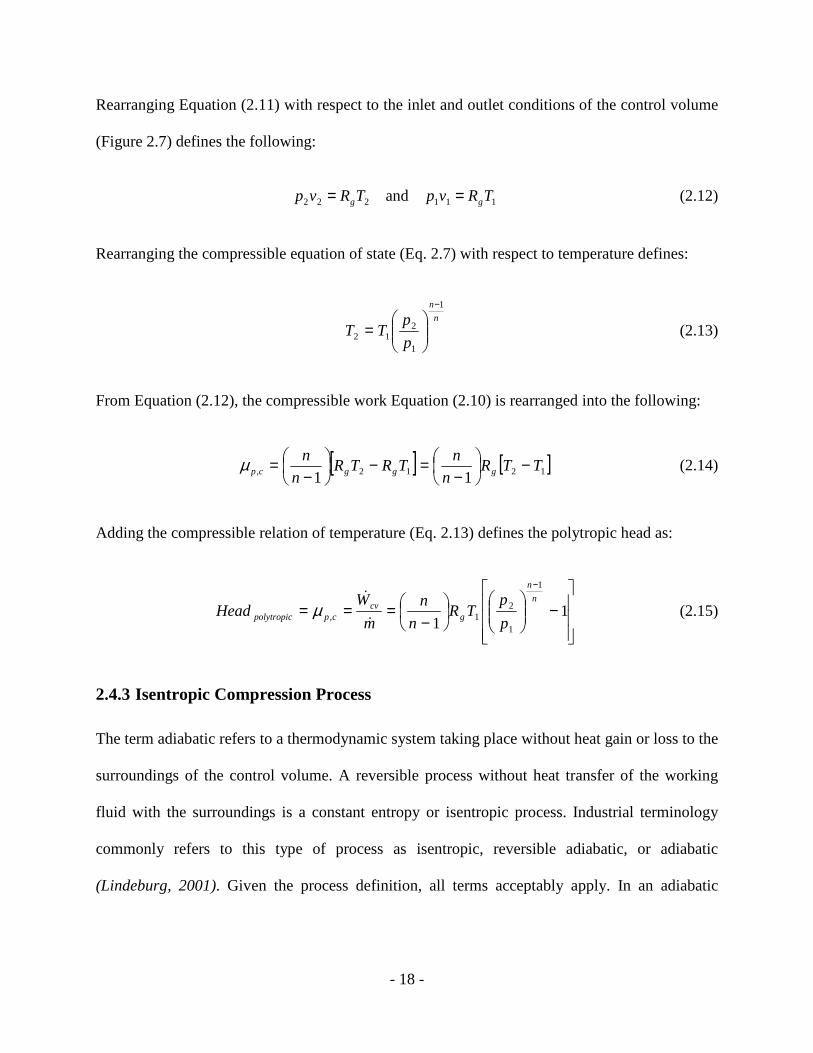
- 18 -
Rearranging Equation (2.11) with respect to the inlet and outlet conditions of the control volume
(Figure 2.7) defines the following:
111222 and TRvpTRvp gg == (2.12)
Rearranging the compressible equation of state (Eq. 2.7) with respect to temperature defines:
n
n
p
pTT
1
1
212
−
= (2.13)
From Equation (2.12), the compressible work Equation (2.10) is rearranged into the following:
[ ] [ ]1212, 11TTR
n
nTRTR
n
ngggcp −
−=−
−=µ (2.14)
Adding the compressible relation of temperature (Eq. 2.13) defines the polytropic head as:
−
−===
−
11
1
1
21,
n
n
gcv
cppolytropic p
pTR
n
n
m
WHead
ɺ
ɺ
µ (2.15)
2.4.3 Isentropic Compression Process
The term adiabatic refers to a thermodynamic system taking place without heat gain or loss to the
surroundings of the control volume. A reversible process without heat transfer of the working
fluid with the surroundings is a constant entropy or isentropic process. Industrial terminology
commonly refers to this type of process as isentropic, reversible adiabatic, or adiabatic
(Lindeburg, 2001). Given the process definition, all terms acceptably apply. In an adiabatic

- 19 -
process, the pressure-volume relation of the compressible gas is defined by the following
equation of state as:
( ) ( ) constant21 == κκ pVpV (2.16)
where the exponent κ is the ratio of specific heats and intrinsically a function of the gas mixture.
Considering Equation (2.16) and the change in pressure-volume between the start and end states
of the compression process defines the equation for isentropic compressible work or isentropic
head. From the work addition to the control volume in Figure 2.7, the enthalpy change is defined
from Equation (2.5), repeated for reference:
( )12, hh
m
W ccv −=ɺ
ɺ
(2.17)
The thermodynamic definition of enthalpy is as follows considering the internal energy and
pressure-volume relation:
pvuh += (2.18)
Substitution of the ideal gas law (Eq. 2.11) in place of the pv term yields:
TRuh g+= (2.19)
The partial derivative with respect to temperature of the enthalpy definition is:
( )TRuhT g+=
∂∂
(2.20)
This defines the isobaric and isochoric heat capacities as follows, respectively:

- 20 -
vv
pp
cT
uc
T
h =
∂∂=
∂∂
, (2.21)
The isobaric term is the specific heat at constant pressure; the isochoric term is the specific heat
at constant volume. The partial derivative of enthalpy with respect to temperature (Eq. 2.20) can
be rewritten in terms of the heat capacities of Equation (2.21) as follows:
gvp Rcc += (2.22)
A term used extensively in gas compression and gas dynamics is the ratio of specific heats. This
is a ratio of enthalpy and internal energy of the gas to form the following:
v
p
c
c=κ (2.23)
Rearranging Equations (2.22) and (2.23) defines the isobaric heat capacity in terms of the ratio of
specific heats and specific gas constant as follows:
gp Rc1−
=κ
κ (2.24)
Relating to the ideal enthalpy difference between the start and end states of the compression
process defines the isentropic compressor work from Equations (2.21) and (2.24) as the
integration with respect to temperature change:
( ) ( )1212, 12
1
TTRdTchh g
T
Tpcs −−
==−= ∫ κκµ (2.25)
Considering a frictionless ideal compressor, the discharge temperature is calculated from the
compressible equation of state (Eq. 2.16) as follows:

- 21 -
κ
κ 1
1
212
−
=
p
pTT (2.26)
Substituting into Equation (2.26) the compression work for pressure in place of temperature
defines the isentropic compressor work equation:
−
−===
−
11
1
1
21,
κκ
κκµ
p
pTR
m
WHead g
cvcsisentropic
ɺ
ɺ
(2.27)
Notably this definition is similar to the polytropic compressor work defined in Equation (2.15).
Replacing the exponent n of the polytropic head equation defines the isentropic head. The two
compression process models were derived from different starting points and result in similar
final equations, differing by the exponent referring to the appropriate compression process.
2.4.4 Conclusion of Compressible Work Discussion
With appropriate gas properties, the polytropic head or isentropic head of the delivered gas is
accurately calculated. The actual compression process is between a polytropic and isentropic
process, thus considering either of these models presents an accurate description of the
compression process. For single-stage compressors, industry typically utilizes the isentropic
process relation for evaluation (Gresh, 2001). The International Organization for Standardization
(ISO) has defined suitable applications for polytropic and isentropic processes regarding the
evaluation of centrifugal compressors in the Turbocompressor Performance Test Code standard
ISO 5389. According to this standard, an isentropic process can be considered as the
compression process model for single-stage compressors with low pressure ratios and when the
compressed fluid exhibits no change in compressibility. This standard further defines the

- 22 -
application of a polytropic process as best suited for moderate to high pressure ratios, multistage
compressors, and applications where the compressed fluid acts as a real gas during the
compression process; hence the compressibility is less than 1.0, (ISO 5389, 2005). Ideal gas and
real gas considerations in PTC10 are defined through the adherence of the gas compressibility
within specified limits of compressor pressure ratio [PTC10-Table 3.3]. Gas compressibility will
be covered in further detail in Section 2.7.6.
2.4.5 Compression Power
The power for an ideal compressor to compress the inlet volume flow to the required
compressible work is termed the gas power. The gas power is calculated via a polytropic process
or isentropic process. Rearranging the Equation (2.5) considering the polytropic head in Equation
(2.15), and inlet mass flow (Equation 2.2) defines the gas power as:
Polytropic Gas Power:
( ) cpinletcpcp VWP ,,, µρ ɺɺɺ == (2.28)
Isentropic Gas Power:
( ) csinletcscs VWP ,,, µρ ɺɺɺ == (2.29)
Considering the compression efficiency with the gas power details the actual gas power:
Actual Polytropic Gas Power:
( )p
cpinletapap VWP
ηµ
ρ ,,,
ɺɺɺ == (2.30)

- 23 -
Actual Isentropic Gas Power:
( )s
csinletasas VWP
ηµ
ρ ,,,
ɺɺɺ == (2.31)
2.4.6 Compressor Polytropic and Isentropic Efficiency
There is an ideal compression process and the actual compression process of the operating
machine. The compression efficiency is established thermodynamically to evaluate a machines
ability to create head and volumetric flow. Both the isentropic and polytropic compression
models have an efficiency relation respective of the process. The efficiency calculation of both
compression models utilizes total or stagnation temperature and pressure of the working fluid,
referencing absolute conditions of the respective measurements. The isentropic efficiency is
defined as follows:
−
−
=
−
1
1
1,,
,2,,
1
1,,
2,,
abst
aabst
abst
abst
s
T
T
p
p κκ
η (2.32)
The polytropic efficiency is defined through the ratio of the polytropic exponent and the
isentropic exponent as:
−
−=
1
1
κκ
η n
n
p (2.33)

- 24 -
2.5 Turbocharger Measurement Locations
According to research performed by Chapman and Mohsen (2000) monitoring performance of
the turbocharger operating on-engine is an important asset to the overall emissions strategy of the
owner/operator. When instrumentation is applied correctly, engine air delivery and efficiency
can be monitored to evaluate the general health of the turbocharger. There is a significant
challenge to collecting accurate field data. In a dedicated test cell, the piping layout to and from
the compressor and turbine can be designed to establish swirl free fluid streams to obtain
accurate pressure and temperature measurements to detail the machine performance. On engine,
the turbocharger piping depends on the air and exhaust manifolds per design by the original
equipment manufacturer and specific installation. The manifolds may vary dramatically between
installations; thus standardizing instrument locations in the field piping would be an impossible
task.
The performance parameters to monitor for important operating information of a turbochargers
health and air supply to the engine are (Chapman, 2000):
• Turbine inlet/outlet pressure and temperature
• Compressor inlet/outlet pressure and temperature
• Compressor delivered airflow
• Ambient conditions collected in the vicinity of the installation (barometric pressure,
temperature, relative humidity)

- 25 -
These performance measurements are best suited at the flange locations on-board the
turbocharger to minimize piping effects, however proper care and calibration of the
instrumentation is required. The flow profiles at the flange locations are unsteady and highly
turbulent. Following a suitable calibration of the instruments applied at these locations with a
well established testing system, the measurements can detail the operating turbocharger
performance on-engine. Figure 2.8 and Figure 2.9 detail the installation locations determined
through the research by Chapman and Mohsen.
Figure 2.8: Compressor Performance Measurement Locations (Chapman, 2000)

- 26 -
Turbine Inlet Temperature and Pressure Turbine Outlet Temperature
Figure 2.9: Turbine Performance Measurement Locations (Chapman, 2000)
2.6 Piping Pressure Losses
The compression pressure ratio between the inlet and discharge conditions at the respective
compressor flanges is a key component of compressible work. If pressure tap locations are
significantly away from the compressor inlet and outlet locations, losses incurred through filter
media, pipe connections, etc. shall be considered in the pressure ratio to accurately evaluate the
overall pressure rise of the compressor. The pressure ratio equation below includes the losses for
the inlet and discharge connection considerations.
lossesinletamb
lossesdis
pp
pp
p
pPR
.
.2
1
2
−+
== (2.34)
To account for piping losses, a differential pressure measuring device could be installed, or the
pressure difference can be calculated from well established equations. In the case of Equation

- 27 -
(2.34) for pipe connections, the losses can be determined by suitable friction factor and pressure
loss evaluation for the flowing fluid.
Relative roughness,ε , is a factor measured as the average size of surface imperfections in the
piping material. The relative roughness for carbon steel piping is 0.0002 ft (Lindeburg, 2001).
The surface roughness coefficient is defined by the relative roughness and the inner diameter of
the piping as follows:
D
ε=tCoefficien Roughness Surface (2.35)
The Reynolds number of the flowing fluid is a ratio of inertial to viscous forces. This is used to
compare the dynamic fluid flow condition between differing piping conditions to ensure the
frictional forces of the flowing boundaries are compared (Munson, 2002):
µ
ρVDRe= (2.36)
For circular piping, the Reynolds number can be defined in terms of the mass flow and reference
geometry in place of the velocity component in Equation (2.36) as follows:
D
mRe
µπɺ4= (2.37)

- 28 -
Figure 2.10: Moody Chart (Munson, 2002)
As detailed by the Moody chart (Figure 2.10), the friction factor, f, of a flowing fluid through a
pipe or conduit depends on the surface roughness coefficient, and the Reynolds number of the
flowing fluid. The friction factor is required for use in pressure drop calculations with the Darcy
Equation (2.42) (Table 2.1).
There has been significant effort to detail the Moody chart in the form of functional equations to
establish friction factor without the requirement of reviewing the chart in Figure 2.10. The
equations in Table 2.1 determine friction factor as a function of the surface roughness
coefficient, and Reynolds number. With the exception of Churchill (Eq. 2.41) and Chen (Eq.
2.39), the equations are for Reynolds numbers greater than 3,500, or above the transition range in

- 29 -
Figure 2.10. Each equation was compared against the Moody chart, finding the accuracy of
Churchill suitable for the analysis for two reasons: larger Reynolds number range and accuracy
with Moody chart when compared against the Chen and Swamee-Jain equations (Eq’s. 2.39 and
2.40). The Colebrook equation (Eq. 2.38) was not evaluated due to iteration requirements of the
friction factor, f.
Table 2.1: Friction Factor and Pipe Pressure Loss
Name Equation Eq. No.
Colebrook 3500,
51.2
7.3
/log0.2
1 ≥
+
−= RefRe
D
f
ε
(Munson, 2002)
(2.38)
Chen (1979)
1
8506.5
8257.2
1log
0452.5
7065.3
/log0.2
18981.0
1088.1
≥
+
−
−=
Re
ReDRe
D
f
εε (2.39)
Swamee-Jain (1976) 3500,
74.5
7.3
/log
25.02
≥
+
= Re
Re
Df
0.9
ε
(2.40)
Churchill (1977)
( )
Reb
Re
Da
RebaRe
f
3753077.3
/ln457.2
1,18
0.8
9.0
12
1
5.11616
12
=
+
=
≥
++
=
ε (2.41)
Darcy
gD
VLfp
pipe
epipe 2
2ρ=∆
(Munson, 2002)
(2.42)

- 30 -
2.7 Thermodynamic and Fluid Properties
The mixture of the working fluid is integral to both the polytropic (Eq’s. 2.15 and 2.27) and
isentropic compression processes in the specific gas constant, gR . With ambient air as the
working fluid of a turbocharger, the two components to consider in the specific gas mixture are
dry air and water vapor. These components define the molecular weight of the gas mixture,
mixMW . The molecular weight of the mixture details the specific gas constant from the universal
gas constant, uR . The specific gas constant of the inlet air considering the molecular weight is
defined as:
mix
ug MW
RR = (2.43)
The specific gas constant is required to accurately calculate the gas density, ratio of specific
heats and compressible work. The ambient condition and mixture will change throughout the
course of a day and therefore are required to detail the gas condition for any compressor
operating point in question. The following sections detail the water vapor, isobaric specific heat,
and ratio of specific heats.
2.7.1 Mole Fraction and Molecular Weight
The molecular weight of the mixture requires the fraction of each component of the mixture; or
the mole fraction. The mole fraction of water vapor is calculated from the actual water vapor,
barometric pressure and saturated vapor pressure as follows:
satamb
vaporv pp
py
−= (2.44)

- 31 -
The water vapor of the mixture is determined from the relative humidity and the saturated vapor
pressure as follows:
satvapor prhp = (2.45)
With the mole fraction of the water vapor, the molecular weight of the mixture is calculated as
follows:
( ) vaporvairi
iivmix MWyMWyMWyMW +−== ∑ v, 1 (2.46)
2.7.2 Saturated Vapor Pressure of Air
The water vapor of the inlet gas changes due to ambient conditions. The amount of water vapor
in the inlet air can be determined from the psychrometric chart or via the saturated vapor from
thermodynamic tables for steam. However, these methods require examining the chart or tables
for each operating data point of the compressor operation. To determine the saturated vapor
pressure without the use of the psychrometric chart or steam table, an algorithm can be used,
provided the accuracy of the calculation method is reasonable.
To determine the saturated vapor pressure of the intake airflow, the steam tables are evaluated
utilizing the relation in Figure 2.11. This is the K-function saturation line established in the
ASME Steam Tables (ASME, 1993).

- 32 -
The K-function is suitable from 32.018°F to the critical temperature of 705.47°F, well outside of
the requirements to detail water vapor of the inlet ambient air, 32°F-120°F. This function
provides a method to calculate the saturated vapor pressure for the operating inlet temperature.
As compared against the steam tables, this function presents an accuracy of +0.003%, -0.004%
for the temperature range of ambient air. Additional methods at slightly reduced accuracy are
detailed for reference in Appendix A: Saturated Vapor Pressure Methods.
Constants for the reduced saturation pressure:
0.6
10975067600.20
16711732.49646225.118
23285504.641706546.168
08023696.26691234564.7
9
987
65
43
21
===
=−==−=
−=−=
k
kk
kk
kk
kk
( ) θσθ −== 1&
27.647 K
KTemp (2.47) & (2.48)
+−
++++++⋅=
92
82
76
55
44
33
22
11
1
1
kkkk
kkkkkk σ
σσσ
σσσσσθ
β (2.49)
Critical pressure: psia235.3208=crp
Saturated vapor pressure: ( ) kepp crsatβ⋅=psia (2.50)
Figure 2.11: K-Function Saturated Vapor Pressure of Water

- 33 -
2.7.3 Isobaric Heat Capacity
The gas mixture at a given state typically requires reviewing data tables for each gas component
of the mixture. As detailed in Equation 2.20, enthalpy changes with respect to temperature can be
detailed as the isobaric heat capacity, pc . The specific heat of dry air and water vapor of the
mixture, mixpc , , will be calculated separately for each component on a molar basis, ipc , . The
specific heat of the mixture on a mass basis is calculated from the component molar specific
heats and the molecular weight as follows:
∑=i iiv
ipmixp MWy
cc
,
,, (2.51)
The specific heat of dry air and water vapor on a molar basis is calculated by the following
polynomial equation (Moran, 1995):
( ) uip RTTTTc 432, εδγβα ++++= (2.52)
The constants of this polynomial and the molecular weights of air and water vapor are defined in
Table 2.2.
Table 2.2: Constants for Specific Heat Polynomial for Dry Air and Water Vapor
Gas Molecular Weight α 310−×β 610−×γ 910−×δ 1210−×ε
Air 28.97 lb/lbmol 3.653 -0.7428 1.017 -0.328 0.02632
Water Vapor 18.0153 lb/lbmol 4.070 -0.616 1.281 -0.508 0.0769
- 34 -
2.7.4 Ratio of Specific Heats
In many cases the water vapor contribution to the mixture is neglected which can be a source of
error in the calculations. With the definition of the specific gas constant and isobaric specific
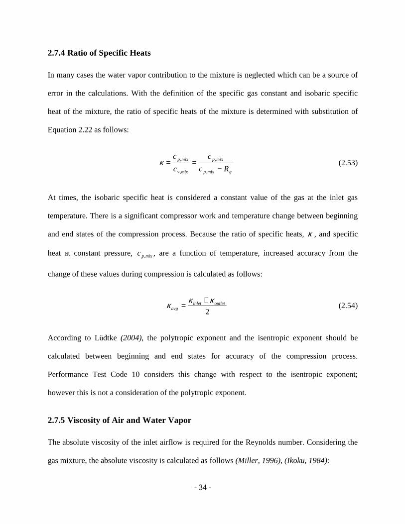
heat of the mixture, the ratio of specific heats of the mixture is determined with substitution of
Equation 2.22 as follows:
gmixp
mixp
mixv
mixp
Rc
c
c
c
−==
,
,
,
,κ (2.53)
At times, the isobaric specific heat is considered a constant value of the gas at the inlet gas
temperature. There is a significant compressor work and temperature change between beginning
and end states of the compression process. Because the ratio of specific heats, κ , and specific
heat at constant pressure, mixpc , , are a function of temperature, increased accuracy from the
change of these values during compression is calculated as follows:
2
outletinletavg
κκκ += (2.54)
According to Lüdtke (2004), the polytropic exponent and the isentropic exponent should be
calculated between beginning and end states for accuracy of the compression process.
Performance Test Code 10 considers this change with respect to the isentropic exponent;
however this is not a consideration of the polytropic exponent.
2.7.5 Viscosity of Air and Water Vapor
The absolute viscosity of the inlet airflow is required for the Reynolds number. Considering the
gas mixture, the absolute viscosity is calculated as follows (Miller, 1996), (Ikoku, 1984):

- 35 -
( )
( ) vaporvairv
vaporvaporvairairv
ii
iiimix
MWyMWy
MWyMWy
MWy
MWy
+−
+−==
∑∑
1
1 µµµµ (2.55)
The absolute viscosity of air is calculated as follows (Tapley, 1990):
( ) ( )( )2
726
ft
seclbf10297.3F006834.0F10659.4 −− ×+°+°×−= TTairµ (2.56)
The absolute viscosity of water vapor is calculated as follows (ASME Steam Tables, 1993):
( ) ( )( )2
726
ft
seclbf10799.1F003306.0F10278.1 −− ×+°+°×= TTvaporµ (2.57)
2.7.6 Gas Compressibility
Gases either follow the ideal gas law or the real gas law, depending on the compressibility for the
pressure and temperature condition of the gas. The critical pressure and critical temperature of a
gas mixture is evaluated as a pseudo-critical condition. The pseudo-critical pressure and
temperatures are comprised of the individual components of the gas.
Pseudo-critical Pressure:
∑=i
icripc pyp , (2.58)
Pseudo-critical Temperature:
∑=i
icripc TyT , (2.59)

- 36 -
The reduced pressure and temperature of the gas mixture are then determined by the following:
Reduced Pressure:
pc
r p
pp = (2.60)
Reduced Temperature:
pc
r T
TT = (2.61)
To verify use of the ideal gas equations for a compressibility of Z=1.0, the reduced temperature
and pressure are utilized in Figure 2.12 to determine the gas compressibility.
Figure 2.12: Compressibility Chart for Reduced Pressure (Moran, 1995)

- 37 -
2.7.7 Total Conditions
Temperature and pressure measurements in the piping system of the turbine and compressor flow
paths are static measurements, defined as: staticT or staticp for the respective measuring location.
The working fluid is in motion at the measuring locations, containing both a static and dynamic
(velocity) component of the temperature and pressure measurements. If the working fluid were
brought to zero velocity and the temperature and pressure measured, a static measurement would
be the total or stagnation measurement of the gas condition. To account for the dynamic
component of the working fluid in motion, the total condition is calculated from the following
equations [PTC10-Eq’s. 5.4.4 and 5.4.6].
dynamic
tabsstaticabst
Vpp
+=
2
2
,,
ρ (2.62)
dynamicmixp
absstaticabst c
VTT
+=
,
2
,, 2 (2.63)
abstg
abstt TR
p
,
,=ρ (2.64)
51,, 10−
− ≤−= ntntError ρρ (2.65)
The total pressure and total density of the working fluid are interdependent making this an
iterative calculation. This is performed with a seed value in the form of static density, and then
iterated to a suitable accuracy for the total pressure and density of the fluid stream. An error
between iterations for density or pressure as detailed in Equation (2.65) provides a suitable
accuracy required for performance considerations. The importance herein is the comparison of
- 38 -
the total conditions of the working fluid independent of the fluid piping and fluid velocity where
measurements are collected. The total conditions of the working fluid are required to accurately
detail compressor work and efficiency.
2.8 Dimensional Analysis and Similitude
A useful method of comparing conditions for numerous engineering models is through the
method of dimensional analysis and similitude. Imagine a physical system (or physical model)
under study with at least five variables contributing to the system, each of which requires
experimentation to determine their contribution. This requires a separate experiment for each
variable, maintaining the remaining variables constant.
Following the individual experimentation, all data from all experiments would require
organization to detail the overall contribution to the model. Therefore a system of five variables
requires five experiments at a minimum and the data between all experiments is segmented. If
the number of variables were to increase, the model testing and evaluation can quickly get out of
hand. Moreover, some variables are interdependent. The viscosity and density of a gas are
temperature dependent; holding temperature constant maintains these important gas conditions
constant as well.
If the experimenter were to evaluate not the individual contribution but the coupled interaction of
the variables relating to the model, experimentation is focused to collecting more useful
information much easier. This is performed through dimensional analysis. Dimensional analysis
is a method of deducing important information of a model given a description by a dimensionally
correct, dimensionless equation of the specific important variables of the model (Langhaar,
1951).

- 39 -
The purpose of dimensional analysis is to provide a means of relating the physical analysis to
useful dimensionless packets of information containing the interaction of the variables of a
model. The method is generally used in fluid mechanics in the exploration of aerodynamics.
Although not obvious, one well known example of this method is the Moody chart (Figure 2.10).
The Moody chart relates the dimensionless friction loss of flow with respect to the surface
roughness coefficient, and the Reynolds number of the fluid and piping. The application of
dimensional analysis is found in the study of problems of stress and strain, fluid mechanics, heat
transfer, electromagnetics and physics (Langhaar, 1951). Additionally, this method can be used
in differential equations in the study of transients as found with natural frequency analysis, and
gas dynamics to mention a few. The full power of this method is realized once applied and
provides a quick method of comparing models without lengthy or tedious calculations.
Though there have been many researchers in this field including the well known works of Lord
Rayleigh, Edgar Buckingham, and Percy Bridgman, the method is commonly referred to as the
Buckingham PI theorem or simply PI theorem (Taylor, 1974), (Munson, 2002). Through the
analysis, the resulting relations are generally referenced as PI terms, noted with the Greek letter
Π. This comes from the paper by Edgar Buckingham (1914) detailing the method which
presented the dimensionless products as Π terms.
To explore this topic we must also define the concept of similitude to consider the geometry, and
dynamic and kinematic conditions required for model testing. The following section details
similitude and the use of dimensional analysis. These concepts develop the fundamental
methodology for evaluating compressor or turbine performance.

- 40 -
2.8.1 Units of Measure
Units of measure can be expressed in terms of established standards and presented numerically to
detail the physical relationship between quantities such as time, length, temperature, mass,
velocity, acceleration, density, etc. Units of measure of length are expressed through established
standards as meters, feet, yards, inches, miles, etc. Area is expressed in terms of length squared,
detailing that a quantity applies to two length dimensions in relation to each other. Area is
expressed in terms of meters², feet², yards², inches², miles², etc². The basic unit or fundamental
dimension of area is therefore length squared (L²); the units of measure provide a physical
comparison to a standard reference measure.
There are different measurement systems, each have relation to each other through standard
universal reference units. The two most recognized measuring systems in general use today are:
the British Gravitational (BG) System, and International System (SI) (Munson, 2002). These
measurement systems provide a means of establishing a numerical value in standard recognized
units of measure.
The effort of evaluating models through dimensional analysis will provide the same overall
results independent of the unit measuring system, provided the fundamental units and resulting
equations are dimensionally homogenous. To be dimensionally homogenous, the unit relations
must follow the same measuring system and basic units, for example: length in terms of feet,
time in terms of seconds, etc. Mixing units (e.g. inches and feet) will result in non-homogeneous
relations that are unit and variable dependent and therefore physically meaningless (Douglas,
1985).

- 41 -
2.8.2 Fundamental Dimensions
Fundamental dimensions are the basic units of length, time, mass and force. In dimensional
analysis two fundamental dimension systems derive the relations to the physical quantities: the
‘force, length, time’ (FLT) system, and the ‘mass, length, time’ (MLT) system.
Applying the fundamental dimensions to the equation of force, maF = , for example provide the
following dimensional groupings:
The FLT system:
( ) ( ) ( )amF LTTFLF 221 −−= (2.66)
The MLT system:
( ) ( ) ( )amFLTMMLT 22 −− = (2.67)
where the indices F, m and a are used to detail the terms of the force equation in the dimensional
groupings. Both groupings are correct considering the fundamental dimensions. Due to
simplicity for the dimensions of a centrifugal compressor, the fundamental dimensions herein
utilize the MLT system. The following sections detail the use and explore the application to a
centrifugal compressor.
2.8.3 Application of Dimensional Analysis to Centrifugal Compressor
As detailed by Buckingham’s theorem (Buckingham, 1914) the number of PI terms, r, to form a
complete description of the model depends on the number of variables to evaluate the model, n,
and the number of fundamental dimensions, m. The number of PI terms that will form from this

- 42 -
are: n - m = r. The theorem states that for a number of related but independent variables, qn’s, of
a model:
( ) 0,,, 321 =nqqqq …φ (2.68)
A solution of the dimensionless products of the qn’s exists as follows:
( ) 0,,, 321 =ΠΠΠΠ r…φ (2.69)
The application to a centrifugal compressor will provide a means to compare between the infinite
combinations of inlet air temperature, pressure, relative humidity, volume flow, compressible
head and speed to create an effective evaluation between differing operating conditions. The
operating variables and fundamental dimensions of a centrifugal compressor are detailed in
Table 2.3.

- 43 -
Table 2.3: Centrifugal Compressor Dimensional Variables
Quantity Variable Unit Dimensions
Compressible Work cµ lbm
lbfft 22 −TL
Inlet Volume Flow Vɺ min
ft 3
13 −TL
Shaft Rotating Speed N RPM 1−T
Compressor Impeller Tip Diameter at Exit 2D ft L
Gas Density ρ 3ft
lbm 3−ML
Absolute Gas Viscosity µ 2ft
seclb 11 −− TML
Fluid Bulk Modulus of Elasticity vE 2ft
lbf 21 −− TML
Surface Roughness of the Internal Passages ε ft L
Since compressible work is the energy per unit weight of the compressible fluid it is appropriate
to define this quantity (cµ ) to include the effects of gravity in the unit dimensions [PTC10-Eq.
5.1-3], (Douglas 1985). This establishes the dimensional groups interrelated to compressible
work as:
),,,,,,( hfv
edcbac EDNV εµρφµ ɺ= (2.70)
hfv
edcbac EDNV εµρµ ɺ= (2.71)

- 44 -
where the alphabetic indices in the above equation are place holders for the evaluation.
Substituting the fundamental dimensions into this relation provides the following:
( ) ( ) hfedcbac LTMLTMLMLLTTLTL )(,,,)(,)(,)(,)( 211131322 1 −−−−−−− −
==µ (2.72)
Note there are seven variables (n) in the potential solution and three fundamental dimensions
(m), defining four dimensionless groups (r) to detail the model. Resolving the indices in the
above relation algebraically while maintaining compressible work and volume flow as a primary
function of compression details the following relation:
( ) ( ) ( ) hfv
efehfeafeaac EDNV εµρµ −−−−−−−−−= 223222ɺ (2.73)
Regrouping each of the indices details the dimensionless groups from the above relation as
follows:
( )
=ΠΠΠΠ=
DDN
E
NDND
V
DNvc ε
ρρµφµ
;;;,,,2223432122
ɺ
(2.74)
Define the impeller tip speed (2u ) as a primary quantity of the impeller diameter at the exit ( 2D )
in Equation (2.75). The added π is a constant and defines the rotational tip speed of the impeller
from the rotational velocity (N ) and impeller diameter (2D ). The constant has no dimensions
therefore maintaining dimensional homogeneity in the group.
( )22 NDu π= (2.75)
with tip speed, this simplifies the groups as a function of compressible work as follows:

- 45 -
=
2
/1
22
/1
222
222
2
;;;
2
Du
E
DuDu
V
u
Ma
v
Re
c ερρ
µµϕψ
ɺ
(2.76)
The variable indices ( MaRe,,ϕψ , ) in the resulting group (Eq. 2.76) detail the variables that will
be utilized to represent each PI term. This statement defines the following important relations:
• Head is a function of the impeller tip speed squared; the head coefficient, ψ .
• Volume flow is a function of the tip speed and impeller exit diameter squared; the flow
coefficient, ϕ .
• The flow, head, and tip speed are coupled through the flow and head coefficient. Plotting the
head coefficient versus flow coefficient therefore defines a dimensionless compressor map
normalized with respect to impeller tip speed. This is the compressor signature of operation,
all operating and specified conditions can be evaluated from this map.
The following also form a relation with the head coefficient:
• Inverse Reynolds number, Re/1 .
• Inverse Mach number squared, 2/1 Ma , or the inverse Cauchy number.
• Surface roughness coefficient, 2/ Dε .
The speed of sound, c, is defined from the bulk modulus and fluid density and can be rearranged
into the more common form found in gas dynamics as:

- 46 -
)(gTRE
c gv κ
ρ== (2.77)
When working with compressible fluids, either the Cauchy number or the Mach number may be
used (Munson, 2002). Although both are acceptable, when working with gas dynamics the Mach
is the more common parameter.
Since all operating parameters of the compressor are defined in the dimensionless groups, the
above relations define the correction methodology for centrifugal compressors. Following the
dimensional relations to maintain dimensional homogeneity, each dimensionless parameter can
be modified adding numerical constants. This is one alteration typically found in turbomachinery
books and references.
2.8.4 Similitude
The concept of similitude provides a method of comparison between fundamentally similar
physical systems by following an appropriate matching of the dimensionless parameters. This
forms a characteristic match of the models. There are three considerations or similarity laws to
maintain when matching conditions between models of comparison: geometry, fluid dynamics,
and kinematics.
A geometric match between models is the highest concern of comparison through dimensionless
parameters. Schlichting details the geometric consideration as providing mechanically similar
flows (Schlichting, 2000). The dimensionless quantities are in relation to a specific impeller
geometry; the impeller shape and blade height which are fixed. If vanes are present in the
discharge diffuser the vane angle must be fixed as well when matching differing operating
conditions.

- 47 -
Matching fluid dynamics considers maintaining the fluid effects of the models. This compares
the Reynolds and Mach numbers between models to ensure the applied fluid forces are
maintained for the deformation of the working fluid through the compressor. This also defines
the density ratio (specific volume ratio) considerations between inlet and outlet conditions of
PTC10. This is provided to maintain consistency between test and specified conditions [PTC10-
Table 3.2].
Finally, to match the kinematics between models, the rotational velocity of the compressor must
be maintained to fulfill the final similarity law. Because of the dependence of compressible head
on the tip speed, the rotational velocity plays a significant role in matching between model
conditions. By matching geometry and either dynamics or kinematics, the third is automatically
matched through the fundamentals of similarity, and ensures similitude and validation of the
models (Munson, 2002).
2.9 Application of Similitude to Centrifugal Compression
For the case of a centrifugal compressor, the primary considerations for matching conditions
between models are geometry and kinematics. The inertial forces of the fluid are much larger
than the viscous forces, establishing large Reynolds numbers for a compressor. This plays a
lesser effect on the model comparison. According to Taylor (1974) model flexibility is key;
insistence on utilizing the Mach number and Reynolds number matching can paralyze the
observer in detailing similitude in this application. Therefore, the machine Mach and Reynolds
numbers are secondary coefficients of similitude of the compressor model. Research in this area
has established technical guidance for considering the Reynolds number and Mach number in
models, and detailed in Sections 2.9.5 and 2.9.6.

- 48 -
For any operating point of interest of the compressor, a set of dimensionless parameters exists to
define the operating point. Secondly, considering the head and flow conditions as primary
operation of the compressor, the following definition (Equation 2.78) is therefore valid to
compare any two operating points between differing inlet density conditions (ambient
conditions) or different compressible fluids. This is termed as test and specified conditions and
the flow and head coefficient match is as follows:
tesptesp ψψϕϕ == & (2.78)
This definition is the fundamental relation required to establish performance comparison
between any two operating conditions of the compressor. Additionally, the Reynolds number and
Mach number must be considered to complete the concept of similitude. The following sections
detail the head and flow coefficients as found in various texts, and detail the Mach number and
Reynolds number relations required to complete the analysis.
2.9.1 Flow Coefficient
Considering a centrifugal compressor the dimensionless parameter for flow is [PTC10-Eq.
5.5.7]:
2
223
23
2 222
1
Du
V
DN
V
ND
m ɺɺɺ===
ππρϕ (2.79)
The flow coefficient is defined in multiple sources with multiple constants, confusing the usage.
Each comparison is valid if data is collapsed and expanded via the same dimensionless
parameter. Table 2.4 details different flow coefficients found from sources referenced herein.

- 49 -
This table details the importance of knowing the flow coefficient utilized to guard against error
in collapsed or dimensionless data.
Table 2.4: Comparison of Compressor Flow Coefficients
Equation No.
Variant Constant, a
Flow Coefficient
2
22
1
Du
V
a
ɺ
Dimensionless? Reference Source
(2.80) 2 2222 Du
Vɺ Yes (PTC10)
(2.81) 4
π 2
224
uD
Vπɺ
Yes (ISO 5389)
(2.82) N/A 2
21
,1.
Dp
Tcm absmixpɺ
Yes (Bathie, 1995)
(2.83) π1
3
2ND
Vɺ Yes
(Japikse, 1997)
(Dixon, 1998)
In the above table, Equation (2.81) is commonly found in European texts, and references the
flow of the compressor in comparison to a similarly sized hole for the term 1
224
−
D
π. Equation
(2.82) includes the isobaric heat capacity and excludes impeller rotational velocity. Error may be
introduced with this relation if the heat capacity or inlet temperature were considered constant, or
if speed were different in the analysis. As found during formation of the dimensionless relations,
Equation (2.83) references the fundamental flow coefficient in Equation (2.74).

- 50 -
2.9.2 Head Coefficient
Similar to the flow coefficient, the head coefficient is defined slightly different by various
sources. The parameter for dimensionless head is [PTC10-Eq’s. 5.1-3 and 5.1T-4]:
2
2ucµψ = (2.84)
Table 2.5 details head coefficients from sources referenced herein, comparing the applied
constant to the coefficient used in the text.
Table 2.5: Compressor Head Coefficient Comparison
Equation No. Variant Constant, a
Head Coefficient
∆2
2
1
u
h
a
Dimensionless? Reference Source
(2.85) 1 22ucµ
Yes (PTC10)
(Japikse, 1997)
(2.86) 2
1
2
22ucµ
Yes (ISO 5389)
(2.87) 2
1
π
( )2
22
/
DN
p ρ∆ Yes (Japikse, 1997)
(2.88) 2
1
π 2
22DN
cµ Yes
(Japikse, 1997)
(Dixon, 1998)
In this table, Equation (2.86) is the ratio of head and the impeller tip speed in a form similar to
the ratio of head to kinetic energy from the energy rate Equation (2.4). Though the velocity

- 51 -
difference between inlet and outlet conditions is considered negligible, this equation follows the
same form due to the importance of tip speed to compressible head. Equation (2.87) defines a
pseudo-head with the term ρ/p∆ . This equation does not utilize the equation of state for gases
(Eq’s. 2.7 and 2.16) and may introduce error with differing gas conditions. As found during
formation of the dimensionless relations, Equation (2.88) references the fundamental head
coefficient in Equation (2.74).
2.9.3 Power Coefficient
The dimensional analysis in Section 2.8.3 can be utilized to form the power coefficient for the
compressor as the head and flow coefficients were formed. This can also be completed by
utilizing the flow and head coefficient (Eq’s. 2.79 and 2.84), and the gas power in Equation
(2.28) or (2.29) as follows.
( ) ( )( )( )22
222., 2 uDuVP pinletcpinletcp ψϕρµρ == ɺɺ (2.89)
Forming the polytropic power coefficient as follows:
3
22
2
,,
2 uD
P
inlet
cp
cp ρ
ɺ
=Ω (2.90)
Similar to the flow and head coefficients, the dimensionless power can be utilized to compare the
gas power signature of the compressor at varying specified density and speed conditions. The
actual gas power can therefore be established as follows:
pinlet
cp
p
p
apuD
P
ηρη 32
22
,
,2
ɺ
=Ω
=Ω (2.91)

- 52 -
2.9.4 Dimensionless Compressor Map
Plotting the dimensionless characteristics of a model presents a method of comparing numerous
details and aspects for evaluating data (Taylor, 1974). As defined above, the head coefficient is a
function of flow coefficient. The isentropic or polytropic efficiency is a function of the flow
coefficient as well. Due to the interdependence of speed, diameter, head and flow, a
dimensionless map can be detailed. Plotting the head coefficient and efficiency versus flow
coefficient for the compressor model and impeller geometry, develops a characteristic curve or
signature of operation for a specific compressor model (Lüdtke, 2004).
2.9.5 Machine Mach Number
As resolved in the dimensionless groups (Eq. 2.76) the Mach number defines an important
parameter to the compressor performance evaluation. In place of the Mach number, a machine
specific Mach number will be defined as the ratio of the tip speed of the impeller, u2, to the inlet
speed of sound, c1, of the working fluid as follows:
1
2
c
uM m = (2.92)
This is a reference Mach number suitable for evaluation of compressor consistency between
model conditions. The name could be suitably termed tip speed Mach number. The importance
lies in the dependency of compressor head and pressure ratio on the impeller tip speed, i.e. the
Mach number (Lüdtke, 2004). Rearranging Equation (2.27) to define the pressure ratio in terms
of the head coefficient and machine Mach number defines the following important relation:
( )[ ]
−+−= 12,
1
2 11 κκ
κψ mcs Mp
p (2.93)

- 53 -
The importance of this equation is the head coefficient is a function of the tip speed, and the
pressure ratio is a function of the Mach number. This defines the importance of the machine
Mach number in the correction procedure and the establishment of speed limits. Following the
guidance of PTC10 requires the difference in machine Mach number between test and specified
conditions, ( )spmtm MM .. − to be within the boundaries plotted in Figure 2.13 to ensure a suitable
comparison between conditions.
Figure 2.13: Allowable Machine Mach Number Departure (ASME PTC10-Fig.3.3)

- 54 -
2.9.6 Machine Reynolds Number
As with the machine Mach number, the Reynolds number is modified to suit the dynamics of the
compressor to represent the fluid friction in the flow passages of the compressor diffuser section
(Lüdtke, 2004). From the dimensionless groups defined in Equation (2.76), the Reynolds number
is modified to accommodate blade height of the impeller at the exit ( 2b ) to the diffuser, viscosity
in terms of the inlet condition, and velocity in terms of the tip speed of the impeller. This defines
the machine Reynolds number as:
1
221
µρ bu
Rem = (2.94)
Following the guidance of PTC10 requires adherence within the boundaries plotted in Figure
2.14 to ensure a suitable comparison between test and specified conditions. This also ensures the
machine Reynolds number between test and specified conditions is within a suitable range for
correcting efficiency and the head coefficient.

- 55 -
Figure 2.14: Allowable Machine Reynolds Number Departure (ASME PTC10-Fig.3.5)
2.9.7 Reynolds Number Correction for Centrifugal Compressors
The two notable variables of the machine Reynolds number are tip speed and kinematic viscosity
( ρµυ /= ), or the absolute viscosity and density. The tip speed must be within the bounds of the
machine Mach number limits (Figure 2.13). It is not feasible or cost effective to maintain the
machine Reynolds number during performance testing (Simon, 1983). Wiesner (1979)
established a method for correcting for the effects of Reynolds number on the head and flow
coefficients, and efficiency. This method has been simplified for use in PTC10 and corrects the
head coefficient and efficiency only, as detailed in Equations (2.95 thru 2.101) [PTC10-Eq’s.
5.6.1-5.6.5]:
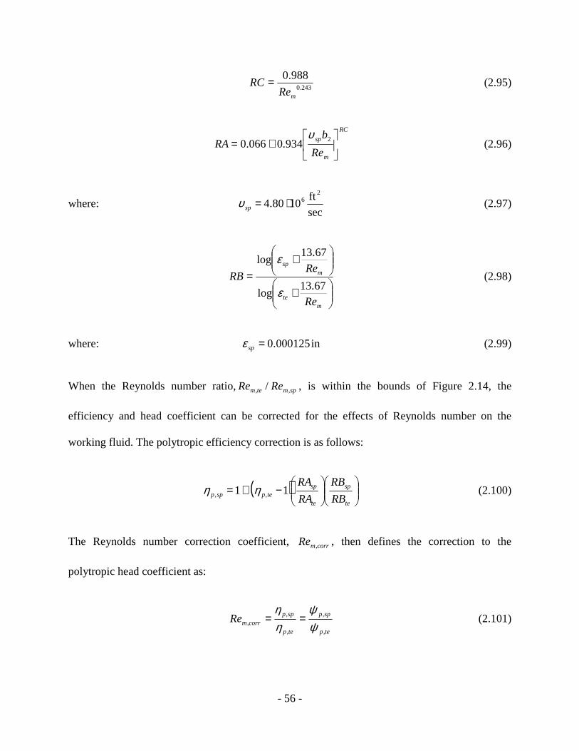
- 56 -
243.0
988.0
mReRC = (2.95)
RC
m
sp
Re
bRA
+= 2934.0066.0
υ (2.96)
where: sec
ft1080.4
26⋅=spυ (2.97)
+
+
=
mte
msp
Re
ReRB
67.13log
67.13log
ε
ε (2.98)
where: in000125.0=spε (2.99)
When the Reynolds number ratio, spmtem ReRe ,, / , is within the bounds of Figure 2.14, the
efficiency and head coefficient can be corrected for the effects of Reynolds number on the
working fluid. The polytropic efficiency correction is as follows:
( )
−+=
te
sp
te
sptepspp RB
RB
RA
RA11 ,, ηη (2.100)
The Reynolds number correction coefficient, corrmRe , , then defines the correction to the
polytropic head coefficient as:
tep
spp
tep
sppcorrmRe
,
,
,
,, ψ
ψηη
== (2.101)

- 57 -
This correction applies to either polytropic or isentropic efficiency, and polytropic or isentropic
head with the corresponding substitution in Equations (2.100) and (2.101).
Although there are a number of additional works from numerous authors in this area, it is beyond
the scope of this work to detail each of the Reynolds number correction methods available for
use today. Interestingly most works in this area root from the Colebrook equation as the basis of
theory and derivation, therefore they agree in principle and not in the finer details of the
application (Wiesner, 1979). Interestingly the Reynolds number correction model for ISO 5389
utilizes a method developed by Strub et al. (1987). Therefore, the Reynolds number correction
methods in the widely referenced compressor performance test codes in the United States and
Europe (PTC10 and ISO 5389, respectively) vary significantly requiring a thorough review of
the open literature, and suitable evaluation of either method prior to use.
2.9.8 Density Ratio
The density ratio between inlet and outlet conditions enables a comparison of compression
between the test and specified gases. PTC10 establishes that the normalized density ratio of test
to specified conditions equals one, with a tolerance of ±4%. The following equation details the
calculation of the specific volume ratio and density ratio for test and specified conditions
[PTC10-Eq. 5.5.5]:
%104%96:Tolerance
i
≤≤
=
=
v
ti
d
spi
d
td
spd
i
v
r
v
v
v
v
v
v
rρ
ρ
(2.102)

- 58 -
2.10 Concluding Remarks
The above literature review leads to the following observations:
• Matching the specified condition of the turbocharger is imperative to verify the design before
installation. The importance of this is to verify the compressor and turbine efficiency which
can have a significant effect on fuel consumption due to their coupling to exhaust gas
backpressure and air delivery to the intake manifold.
• A suitable testing apparatus to accurately detail the information required to define
performance of the turbomachine will utilize significant live computations at time of test.
The calculations to detail the operation must be performed at time of test to ensure an
accurate verification process.
• The required thermodynamic conditions of the inlet air are defined by the temperature,
pressure, and molecular weight detailed through the relative humidity.
• The polytropic and isentropic compression processes are comparable and differ by a
compression exponent representing a machine explicit or gas explicit exponent. The use of
the polytropic equations may significantly limit the use of dimensional analysis because the
specific inlet and outlet gas conditions are collapsed in the compressible work data. Re-
expanding this data into pressure conditions requires the specific polytropic exponent of an
operating point. However, collapsed isentropic head can be re-expanded easily to nearly any
condition in the compressor map because the isentropic exponent is defined by the gas
mixture of interest.

- 59 -
• The use of dimensional analysis provides a method of collapsing and re-expanding collected
data to any condition required for evaluation. This method could be applied at time of test to
verify that all data for a given turbocharger follows a dimensionless characteristic curve or
signature providing a method of quality assurance at time of test. This method may detail any
operating point in the compressor map.
• The effects of the speed variable may be significantly reduced in the Mach and Reynolds
number analysis by testing at the required speed to demonstrate the required head. There
appears to be a significant variation that could be applied to a corrected data set given the
limits of the PTC10 models when the test and specified gas is the same, as in the use of air
for this study.

- 60 -
CHAPTER 3: Test Apparatus
Operating a turbocharger for a large-bore engine offsite requires a specific infrastructure to
supply the required power to the turbocharger for mechanical testing and collecting accurate data
of the performance envelope. With the command of often times certifying performance prior to
field installation, the importance of this task is great. A test cell was designed at the National Gas
Machinery Lab (NGML) of Kansas State University for this specific reason.
3.1 Test Cell Design Requirements
There are a number of systems required to support a turbocharger under test and collect accurate
data. The following list details the systems required:
• Carefully designed piping system and mass flow measuring devices.
• Properly installed and calibrated instrumentation and data collection system.
• Reliable control systems for generating turbine exhaust gas and controlling compressor
discharge pressure.
• Auxiliary systems for heat rejection and bearing lubrication.
• Heavy duty support system for turbocharger under test, and collecting robust vibration data.
ASME has developed several Performance Test Codes (PTC’s) to define best practices for
design configuration and measuring instrumentation to maximize accuracy for performance
measurements of compressors and exhausters. The design of the test cell utilized the following
ASME guidelines to detail the configuration and provide guidance:

- 61 -
• PTC10 on Compressor and Exhausters
• PTC19.5 on Fluid Meters and Flow Measurement
3.2 Exhaust Gas Power System
This section discusses important details of the design as it pertains to the turbocharger testing
required herein. The test cell was designed to deliver a variable flow rate of 3 lb/sec to 30 lb/sec
of compressed air at up to 36 inHgG at 1,000°F exhaust gas temperature to the turbine inlet of a
turbocharger. This provides the power necessary to completely performance map a compressor
and turbine of turbochargers with moderately high turbine inlet pressures. Figure 3.1 details the
system layout of the designed test cell.
A gas turbine engine driving an axial compressor provides the pressurized air stream for the
exhaust gas to the turbocharger turbine. The axial compressor was a modified compressor core
section of an Allison T56 (501D) gas turbine engine. The combustion and turbine section of the
engine were replaced with an aft bearing and discharge air collector as the rear housing. A
coupled 2,400 HP gas turbine engine (GE-T64B) provided the shaft power for the axial
compressor.
The air leaving the compressor discharge collector enters a piping section to measure the mass
air supply to the turbocharger turbine inlet. An inline combustion burner utilizing natural gas
heated the compressed air from the axial compressor to a maximum of 1,000°F, establishing the
independent exhaust gas stream of the test cell. The fuel mass flow rate was measured with an
orifice run to obtain the air fuel ratio and the resulting specific heat and ratio of specific heats for
turbocharger turbine calculations.

- 62 -
Figure 3.1: Turbocharger Test Cell Layout

- 63 -
3.3 Compressor Air System
The airflow drawn into the turbocharger was measured with a high accuracy ASME long radius
flow nozzle. An ambient measuring station details the local weather conditions of the testing
center. Instrumentation in the piping preceding the compressor inlet measures the temperature,
pressure, and airflow to the compressor. To control the compressor pressure rise, two discharge
headers are fitted with precision valves to simulate the restriction an engine would provide. The
discharge headers are instrumented to measure the pressure and temperature rise of the
compressor discharge air.
3.4 Instrumentation and Performance Data
Instrument and measurement accuracy is important for determining machine performance. Per
the guidance of PTC10 to ensure the condition of the compressible gas is accurately measured,
temperature and pressure are measured for the turbine and compressor inlet and outlet flow
streams with four instruments for each location. This is detailed in the process and
instrumentation diagram (P&ID) of Figure 3.2. There is one exception to this statement, due to
piping diameter considerations there are only two pressure transmitters installed in each of the
discharge headers preceding load valve 1 and 2 as detailed in the P&ID.
The compressor discharge and turbine inlet headers were fitted with insulation to minimize heat
loss to the surroundings, and maintain accuracy of the high-temperature measurements. All
instruments are connected to a programmable logic controller (PLC) to continually monitor the
turbocharger under test. In addition to monitoring temperatures and pressures of the turbine and
compressor conditions, the PLC monitors bearing and jacket water conditions for stability and
safety.

- 64 -
Figure 3.2: Turbocharger Test Cell Process and Instrumentation Diagram

- 65 -
3.5 Performance Measurement Data
The complete performance profile of a turbocharger is determined from temperature and pressure
instruments, and the related thermodynamic and fluid mechanic properties. A PLC is
programmed to compute flow and performance calculations of the operating turbocharger and
record the performance data for test reporting. In accordance with the Test Standard for Testing
Large-Bore Engine Turbochargers (Chapman et al. 2005), Table 3.1 details the measurements
required to quantify turbocharger performance. This is also a table form of the P&ID detailed in
Figure 3.2.
Table 3.1: Test Cell Turbocharger Performance Data
No. Description No. Description
1 Barometric Pressure 8 Turbine Inlet Pressure
2 Ambient Temperature 9 Turbine Inlet Temperature
3 Relative Humidity 10 Turbine Discharge Pressure
4 Turbo RPM 11 Turbine Discharge Temperature
5 Compressor Inlet Pressure 12 Turbine Mass Flow Rate (fuel + air)
6 Compressor Inlet Temperature 13 Cooling Water Pressure & Temperature
7 Compressor Dis. Pressure 14 Cooling Water Flow Rate
8 Compressor Dis. Temperature 15 Lube Oil Pressure & Temperature
9 Compressor Mass Flow Rate 16 Lube Oil Flow Rate

- 66 -
CHAPTER 4: Turbocharger Specification
4.1 Specified Engine Design Point
As discussed in Section 2.1.3, the turbocharger is designed to provide airflow to the engine for
exhaust gas scavenging, and to balance the air and exhaust manifold pressures necessary to
achieve the specific trapped mass and deliver the required airflow per the site condition. This
defines the turbocharger design specification, termed the design point. The design point details
the site ambient conditions and inlet air condition to define: density, viscosity, isobaric specific
heat, specific gas constant and the ratio of specific heats. This also details the mass flow and
discharge pressure from the compressor to meet the required engine airflow and manifold
pressure at the design point. The specified condition herein refers to the design point. This details
the gas condition to the compressor inlet utilized for generating the compressor map(s) at
specified conditions. The design point of the compressor of the turbocharger tested is detailed in
Table 4.1.
Table 4.1: Turbocharger Design Point Condition
Measurement Specified Condition
Inlet Temperature [°F] 59.0
Barometric Pressure [psia] 14.70
Relative Humidity [%] 0
Compressor Mass Flow [lb/sec] 12.680
Discharge Pressure [psia] 25.18

- 67 -
4.2 Compressor Design Point
As discussed in Section 2.3, site density controls the amount of delivered mass flow of the intake
volume flow to the compressor. The design point of Table 4.1 must be converted from mass flow
to inlet volumetric flow via the conservation of mass (Equation 2.2) to define the design point in
terms of the compressor operation.
The ambient condition of the test center will not likely equal the ambient condition as defined in
the specification. To develop the required infrastructure to preheat or cool the inlet airflow to the
turbocharger to meet site conditions is cost prohibitive. Because the centrifugal compressor is a
compressible work (head) machine, the site head required for the design point is calculated
through the compressible work Equation (2.27). The head equation includes the site temperature,
specific gas constant, and ratio of specific heats, repeated here for reference:
−
−===
−
11
1
1
21,
κκ
κκµ
p
pTR
m
WHead g
cvcsisentropic
ɺ
ɺ
(2.27)
With the specified gas condition defined in Table 4.1, the required compressible work is equated
via the isentropic definition to utilize the ratio of specific heats exponent for the gas mixture, κ .
The polytropic exponent of Equation (2.8) is defined by the inlet and outlet pressure and
temperatures of the compressor. In a testing environment where the compressor performance is
to be defined and the efficiency is yet unknown, the polytropic head cannot be calculated
accurately prior to testing to define the design point. The results of the calculations to define the
design point and the reference equation numbers herein detailing the specified condition are
listed in Table 4.2.

- 68 -
Table 4.2: Compressor Design Point Calculation for Test
Description Variable Value Eq. No.
Saturated Vapor Pressure [psia] satp 0.2471 (2.50)
Relative Vapor Pressure [psia] vaporp 0 (2.45)
Mole Fraction vy 0% (2.44)
Molecular Weight mixMW 28.97 (2.46)
Specific Gas Constant [ft·lbf/lbm·R] gR 53.34 (2.43)
Isobaric Specific Heat [ft·lbf/lbm·R] mixpc , 186.523 (2.52)
Ratio of Specific Heats κ 1.401 (2.53)
Density [lb/ft³] inletρ 0.07651 (2.11)
Isentropic Discharge Temperature [°F] 2T 145.38 (2.26)
Reduced Pressure [-] rp 0.05 (2.60)
Reduced Temperature [-] rT 2.25 (2.61)
Compressibility [-] Z 1.0 (Figure 2.12)
Inlet Volume Flow [ft³/min]* Vɺ 9,944 (2.2)
Isentropic Head [ft·lbf/lbm]* cs,µ 16,098 (2.27)
* Design point verification inlet volume flow and isentropic head

- 69 -
4.3 Turbocharger Build Data
There are key dimensions of the turbocharger required to define the flow and head coefficients
(Equations 2.79 and 2.84). To correct the performance data from test to specified conditions
requires an evaluation of the machine Mach and Reynolds numbers (Equations 2.92 and 2.94).
There are two physical characteristics for the performance and correction procedure; the impeller
exit blade height, 2b , and the impeller tip diameter, 2D , to define the impeller tip speed 2u .
Table 4.3 details the characteristic data required of the turbocharger for the correction method.
Table 4.3: Turbocharger Build Information
Symbol Description Value
2b Impeller Exit Blade Height 1.079 in
2D Impeller Diameter at Outlet Tip 1.500 ft

- 70 -
CHAPTER 5: Test Cell Data
5.1 Compressor Test Data
The turbocharger was tested and performance mapped in the test center. The compressor was
tested at three operating speeds to collect the raw performance data detailed in Table 5.1 and
Table 5.2. The performance map is established by operating the turbocharger at a set operating
speed, controlled by balancing turbine power to compressor flow. Discharge load valves control
the discharge pressure to establish compressible work (see Figure 3.1). At least four operating
points are collected along a controlled turbocharger speed line for each speed curve. Table 3.1 in
Section 3.5 details the data collected for each operating point.

- 71 -
Table 5.1: Test Cell Data (1 of 2)
Page: 1 of 2
Test Point Number Point 1 Point 2 Point 3 Point 4 Point 5 Point 6 Point 7Ambient Press (psia) 14.4 14.41 14.4 14.4 14.39 14.38 14.38Ambient Temp (F) 59.33 57.38 58.01 58.28 61.29 63.73 64.58Relative Humidity (%) 99.88 99.98 99.99 99.97 97.51 93.27 86.72Turbocharger Speed (RPM) 8043 8007 8068 8040 9900 9901 9974Compressor Inlet Press (psia) 14.03 14.07 14.08 14.1 13.93 13.94 13.96Compressor Inlet Temp (F) 57.65 55.83 56.36 56.88 58.83 60.7 60.87Compressor Outlet Prss-2 (psig) 3.77 3.92 4.13 4.26 6 6.23 6.55Compressor Outlet Temp-2 (F) 107.58 107.55 108.22 110.62 133.48 136.79 139.17Turbine Inlet Press (psig) 3.36 3.16 3.02 2.73 5.26 5 4.8Turbine Inlet Temp (F) 761.08 819.34 914.46 1058.12 762.43 834.37 917.43Turbine Outlet Press (psig) -1.49 -1.49 -1.49 -1.49 -1.49 -1.49 -1.49Turbine Outlet Temp (F) 643.08 703.61 790.38 915.78 637.59 703.23 777.14Lube Oil Inlet Press (psig) 14.22 14.7 14.86 14.47 17.62 17.64 19.19Lube Oil Inlet Temp (F) 148.8 146.87 144.05 148.02 148.1 146.66 147.58Lube Oil Oulet Temp (F) 148.07 146.08 144.22 148.91 149.59 148.65 150.13Water Inlet Press (psig) 32.28 32.4 32.52 32.72 32.36 32.35 32.42Water Inlet Temp (F) 148.13 151.32 152.66 154.77 152.32 152.16 153.37Water Outlet Press (psig) 29.19 29.2 29.33 29.6 29.29 29.33 29.48Water Outlet Temp (F) 156.99 160.83 163.78 168.47 162.5 163.61 166.55
Compressor Airflow (lb/sec) 7.494 6.995 6.745 5.954 9.603 8.976 8.662Lube Oil (lb/sec) 0.26 0.26 0.26 0.27 0.3 0.29 0.32Cooling Water (lb/sec) 8.23 8.28 8.22 8.25 8.19 8.26 8.26Compressor Flow (ACFM) 6082 5645 5448 4810 7830 7338 7081Turbine Flow (ACFM) 0 0 0 0 0 0 0Methane Flow (ACFM) 28 32 35 39 36 40 43Lube Oil (GPM) 2.14 2.19 2.15 2.25 2.48 2.42 2.67Cooling Water (GPM) 60.42 60.79 60.38 60.61 60.14 60.65 60.7Pressure Ratio 1.295 1.303 1.316 1.323 1.464 1.478 1.499Diff. Pressure (inHg) 0.83 1.55 2.26 3.12 1.51 2.5 3.56

- 72 -
Table 5.2: Test Cell Data (2 of 2)
Page: 2 of 2
Test Point Number Point 8 Point 9 Point 10 Point 11 Poin t 12 Point 13 Point 14Ambient Press (psia) 14.37 14.35 14.35 14.35 14.34 14.34 14.35Ambient Temp (F) 64.44 67.54 67.67 67.58 69.67 70.68 71.79Relative Humidity (%) 90.14 89.78 87.95 88.25 84.52 79.36 71.23Turbocharger Speed (RPM) 9888 11852 11982 12017 11915 12026 12138Compressor Inlet Press (psia) 13.99 13.73 13.74 13.73 13.76 13.79 13.83Compressor Inlet Temp (F) 61.55 64.63 64.79 64.75 66.34 66.95 67.26Compressor Outlet Prss-2 (psig) 6.61 8.84 9.03 9.08 9.22 9.72 10.24Compressor Outlet Temp-2 (F) 139.97 171.01 173.92 175.01 176.32 179.82 183.78Turbine Inlet Press (psig) 4.42 7.73 7.92 7.98 7.58 7.43 7.21Turbine Inlet Temp (F) 1024.24 806.15 813.23 815.18 864.05 920.93 1003.36Turbine Outlet Press (psig) -1.49 -1.49 -1.49 -1.49 -1.49 -1.49 -1.49Turbine Outlet Temp (F) 871.21 657.77 661.04 661.78 705.21 755.53 828.27Lube Oil Inlet Press (psig) 18.79 25.34 24.89 24.85 25.19 25.31 25.12Lube Oil Inlet Temp (F) 150.2 145.68 149.25 146.83 151.85 147.6 147.66Lube Oil Oulet Temp (F) 152.54 150.48 153.49 151.61 157.6 154.26 154.94Water Inlet Press (psig) 32.4 32.15 31.99 31.91 31.87 31.87 31.97Water Inlet Temp (F) 154.85 152.68 153.21 153.56 153.28 154.63 155.4Water Outlet Press (psig) 29.75 29.25 29.32 29.58 29.93 30.16 30.74Water Outlet Temp (F) 169.83 165.08 166.31 166.48 167.33 169.75 172.26
Compressor Airflow (lb/sec) 7.91 11.692 11.808 11.912 11.287 10.921 10.578Lube Oil (lb/sec) 0.33 0.38 0.39 0.39 0.41 0.4 0.41Cooling Water (lb/sec) 8.23 8.22 8.19 8.19 8.16 8.22 8.25Compressor Flow (ACFM) 6472 9690 9783 9859 9370 9072 8777Turbine Flow (ACFM) 0 0 0 0 0 0 0Methane Flow (ACFM) 47 49 49 48 50 54 58Lube Oil (GPM) 2.74 3.16 3.24 3.22 3.47 3.37 3.39Cooling Water (GPM) 60.46 60.38 60.15 60.16 59.93 60.43 60.6Pressure Ratio 1.5 1.689 1.702 1.706 1.712 1.745 1.778Diff. Pressure (inHg) 4.46 2.26 2.26 2.24 3.34 4.66 6.17
5.2 Base Compressor Performance Map
This data is plotted as the raw performance map in Figure 5.1, and includes the turbocharger
design point. This plot presents the static polytropic head versus inlet volume flow as a starting
point to detail the correction method. The tested nominal speeds detailed in Figure 5.1 are: 8,000
RPM, 9,900 RPM and 12,000 RPM. The actual operating speeds during testing varied within 1%
of the nominal values. The following sections detail the method of correcting the test data to the
specified condition.

- 73 -
Polytropic Head vs. Inlet Volume FlowRaw Test Data
9949, 162238k
9.9k
12k
-
2,000
4,000
6,000
8,000
10,000
12,000
14,000
16,000
18,000
20,000
4,000 5,000 6,000 7,000 8,000 9,000 10,000 11,000 12,000
Inlet Volume Flow [ICFM]
Pol
ytop
ic H
ead
- S
tatic
, µ
.p.c
.st [
ft·lb
f/lbm
]
8kRPM 9.9kRPM 12kRPM Design Point
Figure 5.1: Compressor Map Prior to Correction
5.3 Compressor Discharge Piping Elbow Losses
Due to space considerations of the test stand configuration, there are piping elbows between the
compressor outlet flange and the discharge pressure measuring station preceding the discharge
load valve (see Figure 5.2). The pressure ratio (PR) defined in Equation (2.34) accounts for
intake and discharge piping losses. A differential pressure transmitter is not installed in the test
cell to measure losses through the elbows. To account for this pressure loss for the pressure ratio
(PR in Figure 5.2), the Darcy Equation (2.42) is utilized. In the test cell, the compressor inlet
piping does not change direction between the compressor inlet pressure measuring station and
the compressor inlet, thus inlet losses for Equation (2.34) are negligible.

- 74 -
The Reynolds number is calculated from Equation (2.37) for the airflow through the compressor
discharge header and outlet viscosity defined by the outlet temperature and Equation (2.55).
Utilizing the Churchill Equation (2.41) the friction factor in the piping is calculated for the Darcy
equation and pressure drop through the connection. Additionally the Darcy equation uses the
equivalent pipe length to define the loss through the elbow connection. The equivalent pipe
length ( eL in Eq. 2.42) for the 12” elbows in Figure 5.2 is 9 ft for use in the pressure loss
calculation (Lindeburg, 2001).
Figure 5.2: Compressor Discharger Header Piping Elbow
Piping Elbow
PR
Inlet Pressure

- 75 -
The resulting pressure losses through the elbow are plotted versus inlet volume flow in Figure
5.3. The elbow pressure losses are added to the pressure ratio Equation (2.34) as lossesdisp . , for
calculating compressor work.
Elbow Pressure Loss vs. Inlet Volume Flow
8k
9.9k
12kDesign Point
0.000
0.005
0.010
0.015
0.020
0.025
0.030
0.035
0.040
4,000 5,000 6,000 7,000 8,000 9,000 10,000 11,000 12,000
Inlet Volume Flow-[ICFM]
Elb
ow P
ress
ure
Loss
[psi
d]
8kRPM 9.9kRPM 12kRPM Design Point
Figure 5.3: Elbow Pressure Loss versus Inlet Volume Flow
5.4 Total Tested Gas Condition
The pressure and temperature measurements collected during the test are static measurements.
The total conditions for pressure and temperature are calculated from Equations (2.62) and (2.63)
to include the dynamic condition of the fluid stream. The total pressure and temperature of the
inlet and outlet, as well as the elbow losses of the discharge piping are included in the head and
efficiency calculations. Figure 5.4 plots the total head and static head versus volume flow in the
compressor map for comparison to evaluate the difference. The total head plotted for the

- 76 -
reference speeds is denoted as 8kRPM.t, 9.9kRPM.t, 12kRPM.t and Design Point.t, and includes
the elbow losses detailed in Figure 5.3. To determine the dynamic contribution to the polytropic
head, the difference in polytropic head between static and total conditions is calculated from
Equation (5.1) resulting in a maximum difference of 2.6% as detailed in the plot.
1Difference,,
,, −=staticcp
totalcp
µµ
(5.1)
Polytropic Head vs. Inlet Volume FlowStatic & Total Conditions
8k
9.9k
12k
Design Point
-
2,000
4,000
6,000
8,000
10,000
12,000
14,000
16,000
18,000
20,000
4,000 5,000 6,000 7,000 8,000 9,000 10,000 11,000 12,000
Inlet Volume Flow-[ICFM]
Pol
ytro
pic
Hea
d (s
tatic
& to
tal)
[ft·lb
f/lbm
]
0.0%
1.0%
2.0%
3.0%
4.0%
5.0%
6.0%
7.0%
8.0%
9.0%
10.0%
Ove
rall
Diff
eren
ce T
otal
to S
tatic
Hea
d [µ
.p.c
.t/µ
.p.c
.st]
8kRPM 9.9kRPM 12kRPM Design Point 8kRPM.t 9.9kRPM.t 12kRPM.t Design Point.t µ.p.c.t/µ.p.c.st
Figure 5.4: Polytropic Head versus Inlet Volume Flow

- 77 -
5.5 Dimensionless Coefficients
Using the equations for the flow and head coefficients, Equations (2.79 and 2.84), establishes a
dimensionless compressor map (Figure 5.5). This dimensionless map is normalized total
polytropic head and volume flow, with respect to speed, and the impeller diameter and geometry.
The head coefficients for all tested operating speeds collapse to a single line, which represents
the head and flow signature for this compressor.
The compressor polytropic efficiency is also plotted versus the flow coefficient. Efficiency is a
function of the flow coefficient and the tip speed. The efficiency for the 8kRPM speed line is
slightly below the efficiency of the remaining speeds of the tested turbo. Matching the flow and
head coefficient between test and specified conditions to verify the specified operating point
(Equation 2.78) ensures the operating efficiency of the compressor is established as expected to
operate on engine at the specified condition. The highlighted region in Figure 5.5 details this
match in the dimensionless compressor map. For the design point tested, the flow and head
coefficients are: φ=0.0396, ψ=0.616; the complete list of dimensionless coefficients are detailed
in Table 5.3.

- 78 -
Dimensionless Results of Test Data
8kRPM 9.9kRPM 12kRPMDesign Point
8kRPM.eff9.9+kRPM.eff
0.20
0.30
0.40
0.50
0.60
0.70
0.80
0.90
0.020 0.025 0.030 0.035 0.040 0.045 0.050
Flow Coefficient [ φ.asme]
Hea
d C
oeffi
cien
t [ψ
.asm
e.sp
]
72%
76%
80%
84%
88%
92%
96%
100%
Pol
ytro
pic
Effi
cien
cy [
η.p
.sp]
8kRPM 9.9kRPM 12kRPM Design Point 8kRPM.eff 9.9+kRPM.eff
Figure 5.5: Head Coefficient and Polytropic Efficiency versus Flow Coefficient
5.6 Corrected Compressor Map
The test data was corrected to the specified condition detailed in Table 4.1 with application of
the Reynolds number correction method (Equations 2.95 thru 2.101). The resulting Reynolds
number correction value, corrm,Re , established a correction range of 0.0% to 0.1% for the test data
head coefficient and polytropic efficiency. Therefore the Wiesner/PTC10 Reynolds number
correction model has a low correction effect on the test cell collected head coefficient and
polytropic efficiency for this turbocharger, between the test and specified condition.

- 79 -
By rearranging the flow and head coefficient of Equations (2.79) and (2.84), the inlet volume
flow and polytropic head were calculated at the specified condition from Equations (5.2) and
(5.3), normalized to 8,000 RPM, 9,900 RPM and 12,000 RPM. Table 5.3 provides a comparison
of the test and corrected speed data. Figure 5.6 plots the corrected head versus volume flow
compressor map.
22,22 DuV spspsp ϕ=ɺ (5.2)
2,2,, spsppspp uψµ = (5.3)
Table 5.3: Test Collected and Corrected Data
Condition Specified[psia] 13.844 14.10 14.70[°F ] 57.984 67.26 59.0
Rel. Humidity [%] 71.23 99.99 0
Flow Coefficient
Head Coefficient Speed.te
Volume Flow.te
Polytropic Head.te.t Speed.sp
Volume Flow.sp
Polytropic Head.sp.t
(te = sp) (sp) [RPM] [ICFM] [ft·lbf/lbm] [RPM] [ICFM] [ft·lbf/lbm]0.0361 0.623 8,043 6,158 7,719 8,000 6,125 7,640 0.0336 0.639 8,007 5,711 7,847 8,000 5,706 7,836 0.0322 0.652 8,068 5,509 8,137 8,000 5,463 8,002 0.0285 0.669 8,040 4,862 8,287 8,000 4,837 8,207 0.0379 0.619 9,900 7,965 11,628 9,900 7,965 11,633 0.0356 0.636 9,901 7,468 11,948 9,900 7,467 11,951 0.0340 0.649 9,974 7,198 12,368 9,900 7,145 12,190 0.0313 0.660 9,888 6,569 12,359 9,900 6,577 12,395
Des. Pt. 0.0396 0.616 11,852 9,949 16,565 11,846 9,944 16,561 0.0395 0.612 11,982 10,042 16,838 12,000 10,058 16,902 0.0398 0.613 12,017 10,137 16,946 12,000 10,123 16,912 0.0381 0.627 11,915 9,616 17,060 12,000 9,685 17,319 0.0364 0.638 12,026 9,294 17,673 12,000 9,274 17,609 0.0349 0.648 12,138 8,980 18,290 12,000 8,878 17,887
Test [min/max]Amb. PressureAmb. Temperature
8kR
PM
9kR
PM
12kR
PM

- 80 -
5.7 Test Cell Compressor Map at Specified Condition
The original turbocharger air specification detailed the design point in terms of mass flow and
discharge pressure. The mass flow is calculated from the design point density in Table 4.2 and
the normalized volume flow from Table 5.3 via the conservation of mass Equation (2.2). The
discharge pressure is calculated by rearranging the polytropic head Equation (2.15) to define this
in terms of pressure from the normalized and corrected polytropic head in Table 5.3 as follows:
Polytropic Head vs. Inlet Volume FlowCorrected Test Data
9944, 16561
8k
9.9k
12k
-
2,000
4,000
6,000
8,000
10,000
12,000
14,000
16,000
18,000
20,000
4,000 5,000 6,000 7,000 8,000 9,000 10,000 11,000 12,000
Inlet Volume Flow [ICFM]
Pol
ytop
ic H
ead
- T
otal
, µ
.p.c
.t [ft
·lbf/l
bm]
8kRPM 9.9kRPM 12kRPM Design Point
Figure 5.6: Corrected Test Cell Compressor Map

- 81 -
1
,,.
,,
,1,,2
,,
11 −
+
−⋅
⋅=
sp
tcpsp
tcpsp
sp
spinletsp
tcp
abstabs TRpp
κηκ
ηκκµ
(5.4)
The resulting mass flow and discharge pressure forms the compressor map corrected to site
conditions in Figure 5.7. This figure also details the design point from the tested conditions
corrected to site conditions. For this turbocharger, the specified design point is 12.68 lb/sec at
25.18 psia. This turbocharger at site conditions will deliver the required mass flow with a slightly
higher pressure of 25.31 psia considering total pressure conditions. Thus the turbocharger
exceeds the required pressure for the design engine mass flow rate.
Mass Flow vs. Discharge PressureCorr: 59°F, 14.70 psia, 0% rh
12.68, 25.31
8k
9.9k
12k
16.00
18.00
20.00
22.00
24.00
26.00
28.00
4.00 5.00 6.00 7.00 8.00 9.00 10.00 11.00 12.00 13.00 14.00
Mass Flow-[lb/sec]
Dis
char
ge P
ress
ure-
Tot
al [p
sia]
8kRPM 9.9kRPM 12kRPM Design Point
Figure 5.7: Compressor Map Corrected to Specified Conditions

- 82 -
CHAPTER 6: Field Data
6.1 Field Installation
For the field installation, the turbocharger was instrumented to collect temperature and pressure
of the inlet and outlet of the turbine and compressor while operating on engine following the
recommendations presented in Section 2.5. Compressor mass flow, operating speed and local
barometric pressure were collected as well. The compressor mass flow utilized a pitot tube to
correlate the delivered mass flow to the engine air manifold. The on-board instrumentation was
calibrated with performance measurements obtained from the test cell. A pictorial schematic of
the instrumented turbocharger is detailed in Figure 6.1. A PLC connected to the instrumentation
recorded measurements to a database thirty times throughout the operating day.
Figure 6.1: Schematic of Field Instrumented Turbocharger

- 83 -
Figure 6.2 shows the field installed turbocharger with the applied instrumentation and instrument
panel housing the instrument wiring, PLC and data recorder. The data utilized herein was
recorded from July through mid September. During this period, the recorder collected over 1,500
data points of the turbocharger operating on-engine. Relative humidity was not part of the field
data set. Inlet relative humidity obtained via historical weather data from
www.weatherunderground.com was applied to the field data by matching the date and time
recorded to the database to account for the inlet gas mixture and water vapor content.
Figure 6.2: Instrumented Turbocharger Installation On-Engine
Instrument Panel Turbocharger

- 84 -
6.2 Raw Field Data
The data recorded during these months provides significant variance of the ambient conditions
compared to the data recorded from the test cell. Table 6.1 details the minimum, maximum and
average ambient conditions for the data recorded during the field study. The field running
condition also varies significantly in comparison to the specified condition for the turbocharger
(see Table 4.1).
Table 6.1: Average Field Conditions
Measurement Minimum Maximum Average
Ambient Temperature [°F] 58 117 84.9
Barometric Pressure [psia] 13.9 14.3 14.19
Relative Humidity 20 100 65
Speed [RPM] 8,337 10,326 9,339
The inlet volume flow and polytropic head were calculated from the field mass flow, pressure
ratio and gas condition for each operating point in the field data set. Figure 6.3 plots the
operating compressor map of the field data. The volume flow varied between 6,743 and 8,844
ICFM to the compressor, the polytropic head varied from 7,942 to 12,478 ft·lbf/lbm. These
values are significantly lower than the design point specified for the turbocharger.

- 85 -
Polytropic Head vs. Inlet Volume FlowWithout Correction
6,000
7,000
8,000
9,000
10,000
11,000
12,000
13,000
14,000
6,000 6,500 7,000 7,500 8,000 8,500 9,000
Inlet Volume Flow [ICFM]
Pol
ytop
ic H
ead
- S
tatic
, µ
.p.c
.st [
ft·lb
f/lbm
]
Figure 6.3: Raw Field Data, Head versus Volume Flow
6.3 Compressor Inlet Pressure and Dimensionless Coefficients
Plotting the flow and head coefficients provides the best manner to evaluate the quality of the
field data. From the field data there were two bands of head and flow coefficients (see Figure
6.5). Reviewing the data, the head coefficient is higher in July, the first month of operation.
Upon inspection of the readings, the inlet pressure transmitter had a variance in comparison to
the barometric pressure ranging from 0.19 to 0.25 psid during this time (see Figure 6.4). Plotting
the difference between barometric pressure and compressor inlet pressure shows in late July
there was a change to the inlet pressure of the compressor, highlighted in Figure 6.4.

- 86 -
Ambient Pressure - Inlet Pressure vs. Time
-0.01
0.05
0.10
0.15
0.20
0.25
0.30
0.35
21-J
un
28-J
un
5-Ju
l
12-J
ul
19-J
ul
26-J
ul
2-A
ug
9-A
ug
16-A
ug
23-A
ug
30-A
ug
6-S
ep
13-S
ep
20-S
ep
Time [day-month]
Am
b. P
ress
ure
- In
let P
ress
ure
[P0-
P1,
psi
d]
P0-P1
Figure 6.4: Difference Ambient Pressure to Compressor Inlet
Evaluating this finding in the dimensionless coefficients shows the same discrepancy as detailed
in Figure 6.5 with the segregated coefficient groups.

- 87 -
Dimensionless Results of Field DataJuly to September
0.50
0.52
0.54
0.56
0.58
0.60
0.62
0.64
0.66
0.68
0.70
0.035 0.036 0.037 0.038 0.039 0.040 0.041 0.042 0.043 0.044 0.045
Flow Coefficient [ φ.asme]
Hea
d C
oeffi
cien
t [ψ
.asm
e.sp
]
July Aug. - Sept.
Figure 6.5: Dimensionless Coefficients from Field Data
Inlet filter losses are a function of volume flow. However, there is no distinct pressure difference
signature in the data as shown in Figure 6.6. The readings before and after July 19th will be
treated separately in the analysis.

- 88 -
Ambient Pressure - Inlet Pressure vs. Inlet Volume Flow
-0.005
0.045
0.095
0.145
0.195
0.245
0.295
0.345
6,00
0
6,50
0
7,00
0
7,50
0
8,00
0
8,50
0
9,00
0
Inlet Volume Flow [ICFM]
Am
b. P
ress
ure
- In
let P
ress
ure
[P0-
P1,
psi
d]
P0-P1
Figure 6.6: Inlet Filter Loss versus Volume Flow
6.4 Correcting to Specified Conditions
The field data segregated for the time periods were corrected to the specified condition following
the procedure in Section 5.7 - Test Cell Compressor Map at Specified Condition. To detail the
speed in the large dataset from the field conditions, the following formula was applied to round-
off trailing digits of the field recorded speed, and provides the specified speed for the correction
procedure.
100100
×
= field
sp
NIntegerN (6.1)

- 89 -
The field data corrected to the specified condition is plotted with respect to mass flow versus
discharge pressure in Figure 6.7. The data from July details a slightly higher discharge pressure
from the compressor. This plot details the operating line of the turbocharger on-engine. The field
data and test cell data are compared in the next section to correlate the two and evaluate where
the turbocharger is operating in comparison to the compressor map collected in the test cell.
Mass Flow vs. Discharge PressureCorr: 59°F, 14.70 psia, 0% rh
16.00
18.00
20.00
22.00
24.00
26.00
28.00
4.00 5.00 6.00 7.00 8.00 9.00 10.00 11.00 12.00 13.00 14.00
Mass Flow-[lb/sec]
Dis
char
ge P
ress
ure
[psi
a]
July Aug. - Sept.
Figure 6.7: Field Data Corrected to Specified Conditions

- 90 -
CHAPTER 7: Correlating Test and Field Data
The corrected data collected in the test cell provided the wide operating range of the compressor
map between high flow and low flow or compressor surge for three different speed lines (Figure
5.7). This was collected in a precisely designed test apparatus to obtain the most accurate
pressure, temperature and air or exhaust gas flow to the turbocharger. Conversely, the
turbocharger operating on-engine as corrected to specified conditions follows one tightly formed
line of mass flow and discharge pressure (Figure 6.7). This section details the comparison of the
data sets, and differences between, finalizing with the verification steps of machine Mach and
Reynolds numbers, and the ratio of densities (Equation 2.102). To begin, the data available
between the two data sets are detailed in Table 7.1 for reference.

- 91 -
Table 7.1: Comparison of Test Cell and Field Data Available
Test Cell Data Field Operating Data
Date / Time Date / Time
Barometric Pressure Barometric Pressure
Compressor Inlet Pressure & Temperature Compressor Inlet Pressure & Temperature
Compressor Dis. Pressure & Temperature Compressor Dis. Pressure & Temperature
Compressor Mass Flow Rate Compressor Mass Flow Rate
Turbine Inlet Pressure & Temperature Turbine Inlet Pressure & Temperature
Turbine Discharge Pressure & Temperature Turbine Discharge Pressure & Temperature
Turbo RPM Turbo RPM
Turbine Mass Flow Rate (fuel + air) None
Cooling Water Pressure & Temperature None
Cooling Water Mass Flow Rate None
Lube Oil Pressure & Temperature None
Lube Oil Mass Flow Rate None
Relative Humidity None
Complete Energy Balance, Turbine & Compressor Performance
Compressor Performance
7.1 Dimensionless Coefficient Comparison
The turbocharger signature operating line formed by the dimensionless flow and head
coefficients between the test and field data provides one method of comparing the data sets.
Figure 7.1 presents the field and test cell dimensionless compressor map with the head
coefficients corrected to specified conditions.

- 92 -
Dimensionless Results Test Data and Field Data July to September
8k9.9k
12k
Design Pointy = 3685.3x3 - 471.88x2 + 14.214x + 0.562
R2 = 0.9178
0.50
0.55
0.60
0.65
0.70
0.75
0.80
0.025 0.027 0.029 0.031 0.033 0.035 0.037 0.039 0.041 0.043 0.045
Flow Coefficient [ φ.asme]
Hea
d C
oeffi
cien
t [ψ
.asm
e.sp
]
July Aug. - Sept. 8kRPM 9.9kRPM 12kRPM Design Point
Figure 7.1: Plot of Compiled Dimensionless Coefficients
Comparing the flow and corrected head coefficients in Figure 7.1 for all data sets shows the
following important points:
1. The test cell data forms a tight signature line within a range of -1.2% to +1.7% for all
data points as compared to a cubic curve fit through the data set.
2. The July field data has a slightly higher head coefficient than this signature line as
expected for higher inlet pressure losses; all data is within +5% of the signature line.
3. The field data head coefficient of Aug. and Sept. is within -3% of the signature line
collected from the test cell.

- 93 -
4. The flow coefficient from the field data is within -5% to +3% of the design point flow
coefficient.
5. The field data falls at the right most edge of the collected compressor map.
6. All head and flow coefficients are within ±5% of the signature line and specified design
point. The turbocharger field data can be compared to the test cell data utilizing
dimensionless coefficients noting the difference bands.
Dimensionless Results Test Data and Field Data July to September
8k
9.9k
12k Design Point
0.016
0.018
0.020
0.022
0.024
0.026
0.028
0.025 0.027 0.029 0.031 0.033 0.035 0.037 0.039 0.041 0.043 0.045
Flow Coefficient [ φ.asme]
Pow
er C
oeffi
cien
t [Ω
.p.c
]
July Aug. - Sept. 8kRPM 9.9kRPM 12kRPM Design Point
Figure 7.2: Polytropic Power Coefficient

- 94 -
Comparing the polytropic power from Equation (2.90) of the test cell and field data sets
establishes the power requirements of the compressor versus flow coefficient in Figure 7.2. This
plot details the following important points:
1. The test cell data falls within -1.2% to 1.7% of the polynomial curve fit of the polytropic
power curve.
2. The July field data has a slightly higher power coefficient line. The July data is within
0.6% to 6.2% of the polynomial curve fit from the test cell data.
3. The field data power coefficient of August and September is within -3.8% to 1.3% of the
polynomial curve fit from the test cell data.
4. The data collected in August and September repeats the power signature collected in the
test cell. Over 1,000 data points confirm this, therefore the earlier data collected in the
July inaccurately provides the field operating performance of the compressor.
To further evaluate power, the actual power coefficient is calculated from Equation (2.91) to
detail the compression power and contribution of compression efficiency. Figure 7.3 presents a
distinct difference between the test and field data, with the two actual power coefficient curves
between -3% to -5% different for all field data. As noted in Equation (2.91) the difference may
be attributed to the compressor efficiency.

- 95 -
Dimensionless Results Test Data and Field Data July to September
8k
9.9k
12k
Design Pointy = -0.7845x2 + 0.6554x + 0.0054
R2 = 0.9897
0.022
0.024
0.026
0.028
0.030
0.032
0.026 0.028 0.030 0.032 0.034 0.036 0.038 0.040 0.042 0.044
Flow Coefficient [ φ.asme]
Act
ual G
as P
ower
Coe
ffici
ent [
Ω.p
/η.p
]
July Aug. - Sept. 8kRPM 9.9kRPM 12kRPM Design Point
Figure 7.3: Actual Gas Power Coefficient
Figure 7.4 shows the field polytropic efficiency ranging from 0% to +6% when compared to the
test cell data. This efficiency difference contributed to the difference in the actual power
coefficient curves in Figure 7.3. This decreased the field actual gas power coefficient signature
due to the efficiency in the denominator of the coefficient.

- 96 -
Dimensionless Results Test Data and Field Data July to September
8kRPM.eff
9.9+kRPM.eff
July
Aug. - Sept.
75.0%
77.0%
79.0%
81.0%
83.0%
85.0%
87.0%
89.0%
91.0%
93.0%
95.0%
0.020 0.025 0.030 0.035 0.040 0.045 0.050
Flow Coefficient [ φ.asme]
Pol
ytro
pic
Effi
cien
cy [
η.p
.sp]
8kRPM.eff 9.9+kRPM.eff July Aug. - Sept.
Figure 7.4: Polytropic Efficiency
From Figure 7.1 and Figure 7.2, the head and power signature lines versus the flow coefficient
provide comparative results between test and field data. These calculations are based on pressure
measurements at the inlet and outlet flange locations of the compressor. The polytropic
efficiency calculated through Equation (2.33) is a thermodynamic relation based on the gas
composition for the ratio of specific heats, and temperature and pressure measurements. The
difference in the efficiency of Figure 7.4 must be a difference in the temperature measurements
between the test cell and field location. In the field installation, the effects of heat transfer from
the compressor casing may influence the field temperature measurement and efficiency, and may
be remedied with the application of insulation (see Figure 6.2). Further analysis of the
temperature measurements are required to determine the root cause of the difference of the

- 97 -
efficiency calculations. This is required to resolve a comparison between data collected as a
baseline from the test cell and utilized as a parameter to monitor the general health of the
compressor operating on engine.
7.2 Compressor Map and Field Data Comparison
The test cell and field data compressor maps (Figure 5.7 and Figure 6.7) corrected to specified
conditions are combined in Figure 7.5. The specified design point volume flow and head is
significantly higher than the field operating data. Extrapolating the design point flow and head
coefficients to the specified conditions (see Section 5.7) for various speeds between 7,000 RPM
to 12,500 RPM creates an estimated operating line of the turbocharger, detailed in Figure 7.5
(Extrapolated Design Point). This line bisects the field data within 3% of the turbocharger
operating line on-engine. The original design point for the turbocharger specification may have
declared a discharge pressure much higher than collected in the field data; however the
turbocharger operated within 3% of the point when expanded for various speeds. The engine
may have operated significantly lower than full power as detailed by the lower field air manifold
pressure.

- 98 -
Mass Flow vs. Discharge PressureCorr: 59°F, 14.70 psia, 0% rh
8k
9.9k
12k12.68, 25.31
y = 0.1029x2 - 0.668x + 17.239
R2 = 1
16.00
18.00
20.00
22.00
24.00
26.00
28.00
4.00 5.00 6.00 7.00 8.00 9.00 10.00 11.00 12.00 13.00 14.00
Mass Flow [lb/sec]
Dis
char
ge P
ress
ure
[psi
a]
Extrapolated Design Point 8kRPM 9.9kRPM 12kRPM Design Point July Aug. - Sept.
Figure 7.5: Corrected Compressor Map of Test and Field Data Sets
7.3 Verifying the Correction Method
The final step of comparing the correction method is to ensure the specified to test conditions
falls within the bounds of the machine Mach and Reynolds number comparison (Figure 2.13 and
Figure 2.14). This is to ensure the tip speed is in compliance with the established code and
correction methodology. Additionally the density ratio between inlet and outlet for test and
specified conditions must be considered. Each of the above are discussed in the following
sections.

- 99 -
7.3.1 Machine Mach Number Verification
The difference of the test cell and field data machine Mach numbers (Equation 2.92) to the
specified Mach number are plotted in Figure 7.6 to compare with limitations of the defined
boundary. For this turbocharger, all corrected data falls well within the required bounds.
To further evaluate this, the range of speed correction with respect to the machine Mach number
were checked to quantify the speed range to the limit boundaries. There were two ranges
checked, the 8kRPM and 12kRPM tested speeds. For the lower operating speed (8kRPM), the
data could be speed corrected between 5,500 to 9,400 RPM and maintain the reference limits.
For the high operating speed (12kRPM), the data could be speed corrected between 10,800 to
12,400 RPM and maintain the reference limits. Although the flow and head coefficients of the
collected data can be used to create virtually any operating speed line of the turbocharger
compressor, the machine Mach number verification helps to limit this practice.

- 100 -
Machine Mach Number Comparison to Permissible Devia tion
-0.20
-0.15
-0.10
-0.05
0.00
0.05
0.10
0.15
0.20
0.4 0.6 0.8 1.0 1.2 1.4 1.6
Machine Mach Number Specified [Mm.sp]
Mac
hine
Mac
h N
umbe
r D
iffer
ence
[M
m.t-
Mm
.sp]
Test Data July Aug. - Sept.
Figure 7.6: Mach Number Verification
7.3.2 Machine Reynolds Number Correction
The machine Reynolds number between test and specified conditions will likely not match, and
is a secondary parameter of the methodology. The field and test cell data sets were corrected
from the operating condition to the specified condition with the PTC10 Reynolds correction
method (Equations 2.95 thru 2.101). Figure 7.7 presents the comparison between test and
specified conditions, detailing all data falls within the boundary limits.

- 101 -
Reynolds Number Comparison to Permissible Deviation
0.01
0.1
1
10
100
1000
1E+04 1E+05 1E+06 1E+07
Reynolds Number at Specified Conditions [Rem.sp]
Rey
nold
s N
umbe
r R
atio
[R
em.te
/Rem
.sp]
Test Data Aug. - Sept. July
Figure 7.7: Reynolds Number Verification
Similar boundary tests of the machine Mach number were checked against the machine Reynolds
number methodology to test the speed range. The range of machine Reynolds Number to
maintain the reference limits as detailed in Figure 7.7 are from 3,000 to 60,000 RPM for the
specified speed and inlet gas viscosity.
To further evaluate the machine Reynolds number correction model, two tested data points with
similar flow coefficients were checked for comparison. These were utilized to evaluate the
correction model for speed and inlet viscosity to compare the resulting corrected polytropic
efficiency. Table 7.2 details the comparison with the design point flow coefficient of 0.03958
and the point near the choke line for the 12kRPM speed line of 0.03952.

- 102 -
Table 7.2: Reynolds Number Evaluation
Flow Coefficient Speed.te Poly.eff Speed.sp
Poly Eff. Corr Diff. in Poly.Eff.
(te = sp) [RPM] [%] [RPM] [%] [%]0.03958 11852 81.16% 12000 81.23% 0.07%0.03952 11982 80.45% 11852 80.50% 0.05%
The resulting difference in the polytropic corrected efficiency varies considerably compared to
the difference in flow coefficients. From this comparison the reduced Wiesner model for
correcting the head coefficient and efficiency to establish performance may be lacking the
expected correction. Therefore a complete evaluation of this model is required before utilization.
Secondly, the Reynolds number correction method contains two constants. The constants detail
that the data of the compressor shall be corrected in comparison to a specified surface roughness
of in 001250.0=ε and specified machine Reynolds number of 26108.4 bRemsp ×⋅= . This
reduces the correction model to a comparison with the established constants.
7.3.3 Density Ratio
The density ratio was calculated for all data for the turbocharger. This results in a range of the
density ratio from Equation (2.102) for all data sets between -0.3% to 2.5%. The density ratio as
calculated for the population of data is within the limits of that specified by the performance
code which is ±4%.

- 103 -
7.4 Summary
This chapter utilized the systematic approach of establishing the compressor signature lines to
overlay the test cell compressor map and field data. This provided a unique comparison of all
data, independent of speed, to determine if a correlation existed. The dimensionless comparison
provides a means of rapidly evaluating the field data with the specified design point of the
turbocharger. The head and flow ranges of the signature lines between the test cell and field data
overlay within ±5% as detailed in this section.
The test cell and field data were corrected to create the mass flow and discharge pressure
compressor map at the specified condition. Plotting the two data sets together established that the
specified design point mass flow and pressure condition was significantly higher than the
comparative data from the turbocharger operating on engine. Of the possible reasons for this
deviation, the engine may not have been operating at full load to achieve the specified design
point during this dataset. If this is the case future data collected when operating with more engine
demand could verify this hypothesis. Extrapolating the design point flow and head coefficient for
a range of speeds created a flow and pressure line that bisected the field collected data. This
supports the assumption of the engine operating at lower demand. Interestingly this extrapolated
line from the design point may provide a means of testing the turbocharger operating flow and
head range as expected on engine.
The machine Mach and Reynolds number limitations verified that all of the data were corrected
within the guidance established in PTC10. From the two verification models, the machine Mach
number is more stringent in limiting the correction range of the collected data for this case study
with air as the working fluid. Rightly so as the pressure rise of the compressor depends on the tip

- 104 -
speed of the compressor. The boundary range limits the ability to correct into operating points of
the compressor without test verification, preventing a method of falsified data. With test and
specified gases that vary more significantly than air, the stringency of this limit may change.
The Reynolds number correction method for efficiency showed a minor influence when
comparing data collected at the same flow coefficient and within 148 RPM. The expectation was
the method would comparatively correct efficiency for speed and viscosity between closely
collected speed data points for the same flow coefficient, however this was not the case. The
compared corrected data exhibited a 0.07% difference in efficiency between the two collected
data points. This minor difference is within the uncertainty of the pressure and temperature
measurements of the efficiency equation. This forms the opinion that a detailed evaluation of the
effects of this correction method should be verified on a number of different test turbochargers to
further detail the application and use in the correction procedure.

- 105 -
CHAPTER 8: Conclusions
The work herein evaluated the background thermodynamics in pursuit of comparing data for a
compressor operated in a precisely designed test cell to data collected from the same
turbocharger operating on engine. The methodology utilized dimensionless coefficients and the
concept of similitude to compare all collected data. Through the evaluation it was found the
quality of the data sets compared well and within reasonable tolerance.
The complete evaluation process of the turbocharger requires measurements of only temperature,
pressure, flow and speed. These measurements define the operation of the turbocharger through
extensive thermodynamic calculations to establish gas conditions, stagnation conditions,
compression processes, and a means for comparing test and specified conditions. The important
takeaway from the evaluation process is the testing setup to establish ambient operating
conditions to mimic that onsite is not required, thus greatly reducing the cost and setup of a test.
Through this methodology ambient conditions that differ significantly between that of a test and
as specified for the design can be accurately simulated to determine the turbocharger onsite
performance.
The importance of this comparison to the operating engine is the fundamental evaluation of the
design point specified to the actual operation on engine. Imagine a simple test with reduced
operating points to only matching the specified design point. Through the methodology here, the
single specified data point collected in the test cell is within a few percent of the inlet volume
flow of the turbocharger operating on engine. If the evaluation process utilized a specified site
mass flow match in place of the volume flow match utilized herein, it would place the design
point significantly away from the real operating point and would be completely dependent on the

- 106 -
inlet density at test day. In the compressor map and dimensionless map, such a match establishes
a different efficiency and may falsely prove turbocharger operation on engine. This establishes
the importance of accounting for matching the site conditions correctly. Determining the field
operation for the test accurately establishes the real on-engine efficiency of the turbocharger. The
result will be found in the engine fuel consumption or turbocharger operating correctly given the
accuracy of the specified point. In contrast, not following the method presented herein could
miss an invalid compressor match during the verification process, nevertheless to be found in an
engine operating with unstable combustion, missed environmental permits, or limited operating
range due to a poorly established turbocharger.

- 107 -
References
American Society of Mechanical Engineers. Performance Test Code on Compressors and Exhausters, PTC 10-1997. New York: ASME, 1998. Print.
American Society of Mechanical Engineers. Steam Tables. Thermodynamic and Transport Properties of Steam. 6th ed. New York: ASME, 1993. Print.
Avallone, Eugene A., Theodore Baumeister III, and Ali M. Sadegh. Mark’s Standard Handbook for Mechanical Engineers. 11th ed. New York: McGraw-Hill, 2007. Print.
Buckingham, Edgar. “On physically similar systems; Illustrations of the use of dimensional equations.” Physical Review Vol. 4, (1914): 345-376. Print.
Bathie, William W. Fundamentals of Gas Turbines. 2nd ed. New York: Wiley 1995. Print.
Chen, Ning H. “An Explicit Equation for Friction factor in Pipe.” Industrial and Engineering Chemistry Fundamentals Vol. 18, (1979): 296-297. Print.
Chapman, K. S., Keshavarz, A., Shultz, J., Sengupta, J., 2005, “Test Standard for Testing Large-Bore Engine Turbochargers,” Gas Research Institute, Report No. GRI-05/0026, Des Plaines, IL.
Chapman, Kirby S. and Omar Mohsen. “Real Time Performance Measurement of an Elliot H-Series Turbocharger.” Proceedings from Gas Machinery Conference, 2000. Gas Machinery Research Council, 2000. Print.
Churchill, Stuart W. “Friction-factor equations spans all fluid flow ranges.” Chemical Engineering Vol. 91, (1977): 91-92. Print.
Daugherty, Robert L., Joseph Franzini. Fluid Mechanics with Engineering Applications. 7th ed. New York: McGraw-Hill, 1977. Print.
Dixon, S. L. Fluid Mechanics and Thermodynamics of Turbomachinery. 4th ed. Boston: Butterworth, 1998. Print.
Douglas, J. F., J. M. Gasiorek, and J. A.Swaffield. Fluid Mechanics. 2nd ed. Great Britain: Bath Press, 1985. Print.
Ehlers, Gary A. “Selection of Turbomachinery – Centrifugal Compressors.” Proceedings of the Twenty-Third Turbomachinery Symposium, September 13-15, 1994. Texas A&M Univ., n.p. Turbomachinery Symposium, 1994. 151-62. Print.
Globe Turbocharger Specialties, Inc. Globe 1215. Web. 24 Nov. 2010. Available at: http://www.globeturbocharger.com/

- 108 -
Gresh, M. Theodore. Compressor Performance: Aerodynamics for the User. 2nd ed. Boston: Butterworth 2001. Print.
International Organization for Standardization. Turbocompressors – Performance Test Code ISO 5389. Switzerland: ISO, 2005. Print.
Ikoku, Chi U. Natural Gas Production Engineering. Malabar: Krieger, 1984. Print.
Japikse, David, Nicholas C. Baines. Introduction to Turbomachinery. Vermont: Concepts ETI, 1997. Print.
Langhaar, Henry L. Dimensional Analysis and Theory of Models. New York: Wiley, 1951. Print.
Lindeburg, Michael R. Mechanical Engineering Reference Manual for the PE Exam. 11th ed. Belmont: Professional Publications, 2001. Print.
Lüdtke, Klaus H. Process Centrifugal Compressors: Basics, Function, Operation, Design, Application. Berlin: Springer 2004. Print.
Moran, Michael J., Howard N. Shapiro. Fundamentals of Thermodynamics. 3rd ed. New York: Wiley, 1995. Print.
Munson, Bruce R., Donald F. Young, and Theodore H. Okiishi. Fundamentals of Fluid Mechanics. 4th ed. New Jersey: Wiley, 2002. Print.
Schlichting, Hermann and Klaus Gersten. Boundary-Layer Theory. 8th ed. Berlin: Springer, 2000. Print.
Shapiro, Ascher H. The Dynamics and Thermodynamics of Compressible Fluid Flow. 2 vols. New York: Ronald, 1953. Print.
Sillman, Sanford. “Overview: Troposphere ozone, smog and ozone-NOx-VOC sensitivity.” Web. 20 Nov. 2010. Available at: http://www-personal.umich.edu/~sillman/ozone.htm
Simon, H. and A. Bülskämper. “On the Evaluation of Reynolds Number and Relative Surface Roughness Effects on Centrifugal Compressor Performance Based on Systematic Experimental Investigations.” Transactions of the ASME Journal of Engineering for Power, paper no: 83-GT-118, (1983). Print.
Strub, R. A., L. Bonciani, C. J. Borer, M. V. Casey, S. L. Cole, B. B. Cook, J. Kotzur, H. Simon, M. A. Strite. “Influence of the Reynolds Number on the Performance of Centrifugal Compressors.” Transactions of the ASME Journal of Turbomachinery Vol. 109, (1987): 541-544. Print.
Swamee, P. K. and A. K. Jain. “Explicit equation for pipe flow problems.” Journal of the Hydraulics Division Vol. 102, (1976): 657-664. Print.

- 109 -
Tapley, Byron, D. Eshbach’s Handbook of Engineering Fundamentals. 4th ed. New York: Wiley, 1990. Print.
Taylor, Edward S. Dimensional Analysis for Engineers. Glasgow: Oxford, 1974. Print.
von Mises, Richard. Mathematical Theory of Compressible Fluid Flow. New York: Dover, 2004. Print.
Wiesner, F. J. “A New Appraisal of Reynolds Number Effects on Centrifugal Compressor Performance.” Transactions of the ASME Journal of Engineering for Power Vol. 101, (1979): 384-395. Print.
Zheng, Ming., Graham T. Reader, J. Gary Hawley. “Diesel engine exhaust gas recirculation - a review on advanced and novel concepts.” Energy Conversion and Management Vol. 45, Issue 6, (2004): 883-900. Print.

- 110 -
Appendix A: Saturated Vapor Pressure Methods
This work utilized the saturated vapor pressure line as detailed by the K-function from the
ASME Steam Tables (ASME, 1993) presented in Figure 2.11. Two alternatives to the K-function
saturation line were evaluated for ambient air conditions between 32.018°F and 128°F in an
effort to reduce the procedure to a more manageable and programmable method for utilization in
a programmable logic controller or quick engineering calculation. These alternative relations
have reduced complexity as compared to the K-function, with slightly reduced accuracy as well.
The alternative calculations and reduced accuracy as compared to the steam tables are as follows:
Table A.1: Alternative Calculations for Saturated Vapor Pressure
Equation Error
( ) ( )
+°+=− 2816.8
18.273
85.17101231.0
FTpsiapsat (A.1)
0.18%
-0.04%
( )( ) ( )aepsiap
FT
sat
a
β
β
61067137.2
49.393
4.7328
⋅=+°
−= (A.2)
0.16%
-0.02%
( )( ) aebarp
KT
sat
a
β
β=
°−= )(/358.52882805.14 (A.3)
(Lüdtke, 2004)
-1.82%
0.41%

- 111 -
Appendix B: Turbocharger Operating Line
Table B.1: Design Testing Line Evaluation Procedure from the Design Point
Step Calculation Required Data
1
Calculate Flow Coefficient
32
1
wheelturboinletsptt
DN
m
πρφφ
ɺ==
Design Point Condition:
- Ambient Temperature
- Barometric Pressure
- Relative Humidity
- Design Point Speed
- Impeller Diameter
- Mass / Volume Flow Rate
2
Calculate Head Coefficient
( ) spt
wheelturbo
in
outinletair
dpDN
p
pTR
ψψπκ
κψ
κκ
≈=
−
⋅−
=
−
2
1
1
1
Design Point Condition:
- R-value Air
- Ratio of Specific Heats
- Inlet Pressure
- Outlet Pressure
- Barometric Pressure
3 Establish volume flow conditions for the design point line or engine load line, jj points in step 4.
4
Calculate test speeds for volume flows
3,,2
1
wheelt
jjinletjjturboD
VNφπ
ɺ=
Volume flows from step 3
5
Calculate discharge pressure for test day condition
( ) 1
.
2.
,2 11 −
+
−⋅=
te
te
te
te
teinletsp
wheeljjturbodpinletjjabs TR
DNpp
κκ
κκπψ
Test Day Condition:
- R-value Air
- Ratio of Specific Heats
- Inlet Temperature
- Speeds from Step 4

- 112 -
Appendix C: Overview of Correction Method
The following pseudo-code details the correction process from the measurements and
dimensions of the compressor, corrected to the specified condition.
Figure C.1: Pseudo-code of Correction Method

- 113 -
Appendix D: Conditions of Ambient Air
The following two plots detail the effects of relative humidity and temperature on the specific
gas constant and the ratio of specific heats.
Specific Gas Constant of Air versus Temperature and Relative Humidity
0%
10%
20%
30%
40%
50%
60%
70%
80%
90%
100%
53.00
53.25
53.50
53.75
54.00
54.25
54.50
54.75
55.00
55.25
55.50
55.75
56.00
-60 -40 -20 0 20 40 60 80 100 120 140
Temperature [°F]
Spe
cific
Gas
Con
stan
t [ft·
lbf/l
b·R
]
Figure D.1: Specific Gas Constant of Air versus Temperature and Relative Humidity

- 114 -
Ratio Specific Heats of Air versus Temperature and Relative Humidity
0%
10%
20%
30%
40%
50%
60%
70%
80%
90%
100%
1.386
1.388
1.390
1.392
1.394
1.396
1.398
1.400
1.402
-60 -40 -20 0 20 40 60 80 100 120 140
Temperature [°F]
Rat
io o
f Spe
cific
Hea
ts (κ
=cp/
cv)
Figure D.2: Ratio of Specific Heats of Air versus Temperature and Relative Humidity

- 115 -
Appendix E: Instrument Uncertainty Analysis
Instrument uncertainty defines the quality of a recorded measurement in comparison to the
absolute value obtainable with a ‘perfect measurement system’. The uncertainty of a
measurement is a function of the installation, instrument accuracy, instrument environmental
effects, data acquisition system, and calculations resulting from the measurement or combination
of measurements. A true uncertainty considers the uncertainty of a population of recordings to
obtain a single averaged, recorded data point, and the uncertainty of the complete data
measurement system. This analysis focuses on the measurement system uncertainty and
considers the uncertainty of the population of data as an absolute recording. Therefore this
considers the quality of the measurement independent of a population of recordings. The general
calculation for uncertainty is as follows:
( ) sinstrumenti NxxxxxU 25
24
23
22
21 ++++= (E.1)
where
1x Instrument full scale accuracy
2x Thermocouple cold junction
3x Accuracy of data acquisition conversion
4x Transmitter accuracy
5x Thermal environment compensation
sinstrumentN Number of installed instruments

- 116 -
The percent uncertainty of the instrument from the above calculation is therefore:
Range Instrument
% ii
UU = (E.2)
Considering the equation for flow metering through a differential nozzle requires evaluation of
the sensitivity of the variables of the flow equation. Therefore, the partial derivative of each
variable is calculated to determine the contribution of each uncertainty to the flow calculation.
The partial derivatives are summarized in the calculations detailed in Figure E.1.
` 14
2
214
ρβ
επP
dCq d
m ∆−
= (E.3)
where
mq Mass flow of differential device
d Nozzle bore diameter
Dd /=β Ratio of bore diameters, nozzle to pipe diameter
dC Nozzle discharge coefficient
ε Gas expansion factor
p∆ Differential pressure across measurement nozzle
nozzleρ Air density upstream of measurement nozzle

- 117 -
Table E.1: Instrument Uncertainty Summary
(See Figure E.1 for Detailed Calculation Procedure)
InstrumentNumber of
Instruments Range AccuracyThermal
Compensation
PLC Analog Conversion Accuracy
Thermal Compensation Uncertainty
Opto Analog Accuracy 1.00E-03Nozzle Inlet Temperature 4 250 0.10% 0.36 2.50E-01 0.75% 1.55%Nozzle Inlet Pressure 2 15 0.25% 0 1.50E-02 0 0.38%Nozzle Diff. Pressure 2 20 0.15% 0 2.00E-02 0 0.25%Compressor Inlet Temperature 4 120 0.10% 0.36 1.20E-01 0.75% 1.64%Compressor Inlet Pressure 4 30 0.25% 0 3.00E-02 0 0.54%Compressor Dis. Temperature 4 500 0.10% 0.36 5.00E-01 0.75% 1.53%Compressor Dis. Pressure 2 100 0.50% 0.00% 1.00E-01 0.03% 0.73%Nozzle - See Calculation for Calculation Uncertainty 0.00E+00 1.04%Compressor Flow - dP 1 100 0.15% 0 1.00E-01 0.02% 0.18%Compressor Flow - Pitot 1 1 1% 0.00E+00 1.00%Compressor Flow 1 1 1.00E-03 1.45%
Tes
t Cel
lF
ield
F
low

- 118 -
Figure E.1: Uncertainty Calculations

- 119 -

- 120 -

- 121 -

- 122 -