correlating tropospheric column ozone with tropopause ... · aura-omi satellite data ... ing events...

Atmos. Chem. Phys., 10, 9681–9688, 2010www.atmos-chem-phys.net/10/9681/2010/doi:10.5194/acp-10-9681-2010© Author(s) 2010. CC Attribution 3.0 License.

AtmosphericChemistry

and Physics

Correlating tropospheric column ozone with tropopause folds: theAura-OMI satellite data

Q. Tang and M. J. Prather

Department of Earth System Science, University of California, Irvine, California, 92697, USA

Received: 4 May 2010 – Published in Atmos. Chem. Phys. Discuss.: 16 June 2010Revised: 29 August 2010 – Accepted: 20 September 2010 – Published: 12 October 2010

Abstract. The geographic and temporal variations in tro-pospheric and stratospheric ozone columns from individ-ual swath measurements of the Ozone Monitoring Instru-ment (OMI), on the NASA Aura spacecraft, are reason-ably well simulated by the University of California, Irvine(UCI) chemistry transport model (CTM) using 1◦

×1◦×40-

layer meteorological fields for the year 2005. From theCTM we find that high-frequency spatial variations in tro-pospheric column ozone (TCO), including around the jetstreams, are not generally correlated with variations in strato-spheric ozone column, but instead are collocated with fold-ing events involving stratospheric-origin, high-ozone layersbelow the tropopause. The CTM fold events are verified inmany cases with available ozone sondes. Using the OMILevel 2 profiles, and defining tropopause height from ourCTM using the European Centre for Medium-Range WeatherForecasts (ECMWF) fields, we find that most of the vari-ations in TCO near CTM folding events are also not cor-related with those in stratospheric ozone column. A largefraction of the OMI TCO variance is accurately simulated bythe CTM where the variance is significant, especially alongthe subtropical jets. The absolute tropospheric columns fromOMI and CTM agree swath-by-swath, pixel-by-pixel within±5 Dobson Units (DU) for most cases. Notable exceptionsare in the tropics where neither the high ozone from biomassburning nor the low ozone in the convergence zones over thePacific is found in the OMI observations, because of OMI’sinsensitivity to the lower troposphere. Another difference isidentified with the OMI profiles near the southern subtropicaljet. The CTM has a high bias in stratospheric column out-side the tropics, due to problems previously identified with

Correspondence to:Q. Tang([email protected])

the stratospheric circulation in the 40-layer meteorologicalfields. Overall, we identify ozone folds with short-lived fea-tures in TCO that have scales of a few hundred kilometres asobserved by OMI.

1 Introduction

Stratosphere-troposphere exchange (STE) plays an impor-tant role in determining the chemical composition in the at-mosphere, bringing O3-rich stratospheric air into the tropo-sphere (Danielsen, 1968), affecting the oxidative capacity ofthe atmosphere (Levy, 1972; Crutzen, 1973). Many stud-ies have aimed at quantifying the STE flux (e.g.,Danielsen,1968; Holton et al., 1995; Appenzeller et al., 1996; Olsenet al., 2003; Sprenger et al., 2003; Stohl et al., 2003; Jaegerand Sprenger, 2009). This is a global problem that requiresglobal observation and modelling. We identify STE O3 fluxwith many tropopause folds (TF) in our chemistry trans-port model (CTM) and then show that these folds are ob-served as variations in tropospheric column ozone (TCO) ona daily global basis by the Aura Ozone Monitoring Instru-ment (OMI) satellite measurement.

Tropopause folding in the vicinity of both subtropical andpolar jets have been observed to be a particularly importantprocess leading to STE (e.g.,Danielsen, 1968; Lamarque andHess, 1994; Beekmann et al., 1997; Baray et al., 2000; Trauband Lelieveld, 2003). TFs facilitate a great amount of STEflux, although not all of the material in the folds enters thetroposphere (Hsu et al., 2005). We have looked for evidenceof TF in the four Aura ozone instruments. In our model andozone sonde data most folds are about 1–2 km thick and oc-cur between 150–300 hPa. The Microwave Limb Sounder(MLS) with only three levels below 100 hPa is unable to

Published by Copernicus Publications on behalf of the European Geosciences Union.

http://creativecommons.org/licenses/by/3.0/

9682 Q. Tang and M. J. Prather: OMI tropopause folds

resolve most folds. The High Resolution Dynamics LimbSounder (HIRDLS) with higher vertical resolution still doesnot have enough useful data below 150 hPa. We are leftwith identifying TF in the tropospheric data from the Tro-pospheric Emission Spectrometer (TES) and OMI. Neitherinstruments, however, can resolve most folds vertically and,thus, identification requires matching geographic anomalypatterns in the tropospheric columns. The wide swath datafrom OMI is our first choice and is analysed here.

First, we evaluate the CTM using ozone sonde data, find-ing good agreement for the 638 exact matches between 35◦ Sand 40◦ N in the year 2005. The criteria of detecting TF inthe CTM are described at the end of Sect.2. Good consis-tency between the OMI and CTM TCO and total ozone isshown in Sect.3. In Sect.3.1, we find TFs are correlatedwith anomalies in TCO but not in total ozone. Furthermore,we try to link TCO anomalies with STE O3 flux in Sect.4and find good correlation in the vicinity of subtropical jets,but not in high latitudes.

2 Chemistry transport model and ozone sondes

The chemistry transport model (CTM) is driven by pieced-together, spun-up forecasts from the Integrated Forecast Sys-tem of the European Centre for Medium-Range WeatherForecasts (ECMWF) developed in collaboration with Uni-versity of Oslo. The CTM is run at 1◦×1◦

×40-layerspatial resolution with∼1 km vertical resolution near thetropopause. The uppermost layer is exceedingly coarse (2–22 hPa). The chemistry scheme is a combination of theASAD software package for the troposphere (Carver et al.,1997; Wild et al., 2003) and linearized ozone scheme for thestratosphere (Linoz version 2) (Hsu and Prather, 2009). TheASAD algorithm has been recently rewritten at UCI, includ-ing the steady-state assumptions used to optimize the solver.We use the Year-2000 emissions from the EU Quantifyingthe Climate Impact of Global and European Transport Sys-tems (QUANTIFY) project, with monthly biomass burningemissions from the average multi-year (1997–2002) GlobalFire Emissions Database (Hoor et al., 2009). LightningNOx (NO+NO2) is scaled linearly to the deep convectivemass flux with an annual total of 5.0 Tg N yr−1 for the year2005. The resulting tropospheric ozone is typical: North-ern Hemisphere (NH), 42.8 Dobson Units (DU); SouthernHemisphere (SH), 32.8 DU; STE flux, 590 Tg yr−1; surfacedeposition, 760 Tg yr−1; and, thus, net photochemical pro-duction, 170 Tg yr−1. Due to poor resolution in the upperstratosphere, the 40-layer meteorological fields (only versionavailable at 1◦×1◦) are anomalously high in the STE fluxby about 15% compared to similar 60-layer meteorologicalfields (Hsu and Prather, 2009).

To simulate the Aura ozone instruments, we store theCTM O3 in 3-D for each OMI swath, saving two datasets30-min apart to interpolate the exact time for each pixel

(∼63 GB yr−1 in real*4 format). We also save 65◦ S–65◦ Nevery two hours to match ozone sondes (∼29 GB yr−1 inreal*4 format). Therefore, we can generate individual ob-servations.

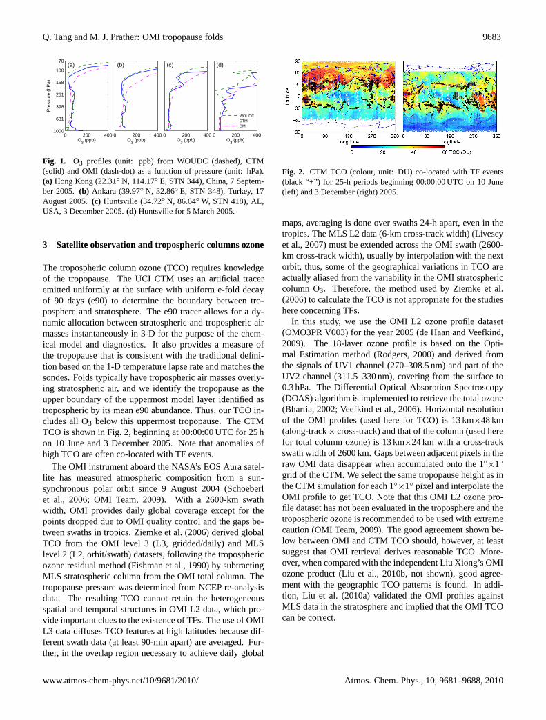
A critical evaluation of the modelled ozone, particularlywith regard to TFs is found with the ozone sonde measure-ments. In this test we restrict our comparison range from35◦ S to 40◦ N where the CTM predicts the preponderance ofTF, giving 638 World Ozone and Ultraviolet Radiation DataCentre (WOUDC) ozone sondes from 20 stations for 2005(HKO et al., 2009). Ozone sondes have much finer verti-cal resolution than the CTM. Figure1 shows four examplesfrom Hong Kong (Fig.1a), Ankara (Fig.1b), and Huntsville(Fig. 1c, d). The CTM (blue solid line) agrees well withsonde (green dash line) in Fig.1a, except for the overestima-tion in the boundary layer, due to the smoothing of the HongKong pollution plumes on our 100-km grid. Both CTM andsonde show fold structure near 251 hPa, but the CTM missesthe fine structure reported by sonde at 140 hPa, leading toan offset of 50 ppb (parts per billion, nanomoles per mole ofair) in the profile. In Fig.1b, CTM and sonde closely matchwith a O3 maximum at 400 hPa. In Fig.1c, model and sondeare similar from the surface to 250 hPa with a fold structurenear 158 hPa, although of different magnitude. Compari-son in Fig.1d is the worst: CTM predicts an increase whilesonde detects a decrease around 250 hPa; fold structure canbe found in both from 100–158 hPa, but the patterns differenormously. Overall, we grade 50% of these 638 compar-isons as “A” (e.g., Fig.1a, b), 30% as “C” (e.g., Fig.1c), and20% as “F” (e.g., Fig.1d).

The reported OMI profiles (de Haan and Veefkind, 2009)include 3–6 tropospheric layers, but only contain approxi-mately one degree of freedom for the signal in the tropo-sphere. Thus, TF detected by OMI could at best be de-tected as an enhancement somewhere in column, most likelyin the troposphere, but not as a fold resolved by sonde orCTM. OMI profiles (magenta dot dash line) generally under-estimate ozone values in the lower and middle troposphere,but overestimate them in upper troposphere and lower strato-sphere (Fig.1).

An objective criteria to identify TF is developed for theCTM based on subjective evaluations of the 638 sonde com-parisons. TFs are defined in a boolean sense (Yes or No) fromthe vertical profile of O3 abundance: starting above 5 km,once the O3 exceeds 80 ppb and then within 3 km abovedecreases by 20 ppb or more to a value less than 120 ppb.Note that TF detection depends in part on the vertical res-olution of the CTM. Given this experiment, the uppermosttropospheric layer in fold must be at least 1 km thick. Alsonote that by these criteria, TFs can be caused by STE eventsand/or biomass burning. For example, Fig.2 shows simu-lated global TCO maps for two “daily” (25-h periods) OMIswath observations, in which the 1◦

×1◦ pixels with a TFevent are marked with “+”.

Atmos. Chem. Phys., 10, 9681–9688, 2010 www.atmos-chem-phys.net/10/9681/2010/

Q. Tang and M. J. Prather: OMI tropopause folds 9683

0 200 400

70

100

158

251

398

631

1000

O3 (ppb)

Pre

ssur

e (h

Pa)

0 200 400O

3 (ppb)

0 200 400O

3 (ppb)

0 200 400O

3 (ppb)

WOUDCCTMOMI

(a) (b) (c) (d)

Fig. 1. O3 profiles (unit: ppb) from WOUDC (dashed), CTM(solid) and OMI (dash-dot) as a function of pressure (unit: hPa).(a) Hong Kong (22.31◦ N, 114.17◦ E, STN 344), China, 7 Septem-ber 2005. (b) Ankara (39.97◦ N, 32.86◦ E, STN 348), Turkey, 17August 2005.(c) Huntsville (34.72◦ N, 86.64◦ W, STN 418), AL,USA, 3 December 2005.(d) Huntsville for 5 March 2005.

3 Satellite observation and tropospheric columns ozone

The tropospheric column ozone (TCO) requires knowledgeof the tropopause. The UCI CTM uses an artificial traceremitted uniformly at the surface with uniform e-fold decayof 90 days (e90) to determine the boundary between tro-posphere and stratosphere. The e90 tracer allows for a dy-namic allocation between stratospheric and tropospheric airmasses instantaneously in 3-D for the purpose of the chem-ical model and diagnostics. It also provides a measure ofthe tropopause that is consistent with the traditional defini-tion based on the 1-D temperature lapse rate and matches thesondes. Folds typically have tropospheric air masses overly-ing stratospheric air, and we identify the tropopause as theupper boundary of the uppermost model layer identified astropospheric by its mean e90 abundance. Thus, our TCO in-cludes all O3 below this uppermost tropopause. The CTMTCO is shown in Fig.2, beginning at 00:00:00 UTC for 25 hon 10 June and 3 December 2005. Note that anomalies ofhigh TCO are often co-located with TF events.

The OMI instrument aboard the NASA’s EOS Aura satel-lite has measured atmospheric composition from a sun-synchronous polar orbit since 9 August 2004 (Schoeberlet al., 2006; OMI Team, 2009). With a 2600-km swathwidth, OMI provides daily global coverage except for thepoints dropped due to OMI quality control and the gaps be-tween swaths in tropics.Ziemke et al.(2006) derived globalTCO from the OMI level 3 (L3, gridded/daily) and MLSlevel 2 (L2, orbit/swath) datasets, following the troposphericozone residual method (Fishman et al., 1990) by subtractingMLS stratospheric column from the OMI total column. Thetropopause pressure was determined from NCEP re-analysisdata. The resulting TCO cannot retain the heterogeneousspatial and temporal structures in OMI L2 data, which pro-vide important clues to the existence of TFs. The use of OMIL3 data diffuses TCO features at high latitudes because dif-ferent swath data (at least 90-min apart) are averaged. Fur-ther, in the overlap region necessary to achieve daily global

Copernicus Publications Bahnhofsallee 1e 37081 Göttingen Germany Martin Rasmussen (Managing Director) Nadine Deisel (Head of Production/Promotion)

Contact [email protected] http://publications.copernicus.org Phone +49-551-900339-50 Fax +49-551-900339-70

Legal Body Copernicus Gesellschaft mbH Based in Göttingen Registered in HRB 131 298 County Court Göttingen Tax Office FA Göttingen USt-IdNr. DE216566440

Page 1/1

Fig. 2. CTM TCO (colour, unit: DU) co-located with TF events(black “+”) for 25-h periods beginning 00:00:00 UTC on 10 June(left) and 3 December (right) 2005.

maps, averaging is done over swaths 24-h apart, even in thetropics. The MLS L2 data (6-km cross-track width) (Liveseyet al., 2007) must be extended across the OMI swath (2600-km cross-track width), usually by interpolation with the nextorbit, thus, some of the geographical variations in TCO areactually aliased from the variability in the OMI stratosphericcolumn O3. Therefore, the method used byZiemke et al.(2006) to calculate the TCO is not appropriate for the studieshere concerning TFs.

In this study, we use the OMI L2 ozone profile dataset(OMO3PR V003) for the year 2005 (de Haan and Veefkind,2009). The 18-layer ozone profile is based on the Opti-mal Estimation method (Rodgers, 2000) and derived fromthe signals of UV1 channel (270–308.5 nm) and part of theUV2 channel (311.5–330 nm), covering from the surface to0.3 hPa. The Differential Optical Absorption Spectroscopy(DOAS) algorithm is implemented to retrieve the total ozone(Bhartia, 2002; Veefkind et al., 2006). Horizontal resolutionof the OMI profiles (used here for TCO) is 13 km×48 km(along-track× cross-track) and that of the column (used herefor total column ozone) is 13 km×24 km with a cross-trackswath width of 2600 km. Gaps between adjacent pixels in theraw OMI data disappear when accumulated onto the 1◦

×1◦

grid of the CTM. We select the same tropopause height as inthe CTM simulation for each 1◦×1◦ pixel and interpolate theOMI profile to get TCO. Note that this OMI L2 ozone pro-file dataset has not been evaluated in the troposphere and thetropospheric ozone is recommended to be used with extremecaution (OMI Team, 2009). The good agreement shown be-low between OMI and CTM TCO should, however, at leastsuggest that OMI retrieval derives reasonable TCO. More-over, when compared with the independent Liu Xiong’s OMIozone product (Liu et al., 2010b, not shown), good agree-ment with the geographic TCO patterns is found. In addi-tion, Liu et al. (2010a) validated the OMI profiles againstMLS data in the stratosphere and implied that the OMI TCOcan be correct.

www.atmos-chem-phys.net/10/9681/2010/ Atmos. Chem. Phys., 10, 9681–9688, 2010





Page 1/1

Fig. 3. Swath-by-swath comparison of total column O3 (unit: DU)from OMI (top) and CTM (bottom) for 10 June 2005 (left) and 3December 2005 (right).

3.1 Swath-by-swath comparison

OMI L2 swath data allows us to study TFs on an hourly basis,which is important since they are not static over a day. Gen-erally there is very good agreement between the modelledand measured ozone columns, both total and TCO. Impor-tantly, the TCO anomalies are not correlated with total ozoneanomalies which would be the case if we were aliasing uppertropospheric meteorologies (ridges and troughs) as STE in-trusions. Thus, we find TFs drive variations in TCO but notin total column.

Analysis of the 25 h of swaths beginning at 00:00:00 UTCfor 10 June are shown in Fig.3a, c and Fig.4a, c and for 3December in Fig.3b, d and Fig.4b, d. The total columnozone for OMI is shown in Fig.3a, b, while that for theCTM is in Fig. 3c, d. The UCI CTM successfully repro-duces the patterns, but overestimates in most extra-tropicalregions by about 15%. We recognized this problem with thestratospheric circulation of the 40-layer ECMWF wind field(Hsu and Prather, 2009).

The TCO patterns (Fig.4) are also quite similar, withsmaller absolute error than for total ozone. In both OMI andCTM a band of high TCO (∼40 DU) at 30◦ N spreads fromthe Eastern Asia, across the Pacific and North America, tothe central Atlantic. In December, the maximum regions tothe east of Australia also appear in both. At 28◦ S, however,OMI TCO has a narrow band of high TCO (∼45 DU) acrossall longitudes, which seems unphysical and has no analog inthe CTM. One apparent reason for this difference is the useof a fixed climatological profile for the a priori in the retrieval(de Haan and Veefkind, 2009). The O3-rich areas over tropi-cal Africa and South America due to biomass burning in theCTM are missing in OMI, most likely because OMI is less




Page 1/1

Fig. 4. Swath-by-swath comparison of tropospheric column O3(TCO in DU) from OMI (top) and CTM (bottom) for 10 June 2005(left) and 3 December 2005 (right).

sensitive to lower tropospheric O3 (Zhang et al., 2010). Like-wise, OMI does not detect the very low TCO over equatorialwestern and central Pacific, where the low O3 abundancesare predominantly near the surface.

3.2 Bias and variability in the CTM tropospheric ozone

Analysis of the time series of TCO for the months of Juneand December are shown in Figs.5 and 6, respectively.The patterns of the monthly mean differences (CTM−OMI)show smooth large-scale features that change only little frommonth to month as shown in Figs.5c and6c. For most of thedaylit globe (56% in June and 65% in December), the differ-ences are within±5 DU. Larger, positive biases exist overAfrica and South America. In June, the greatest differencesare located at southern Africa, while in December large bi-ases concentrate over central Africa, following the seasonal-ity of biomass burning. Likewise, the differences over SouthAmerica are more enhanced in December than in June. Sig-nificant low biases occur over western equatorial Pacific forboth months related to the ozone loss in the marine boundarylayer, where the CTM matches the typically low 5–15 ppbobserved in the tropical Pacific (Davis et al., 1996; Crawfordet al., 1997; Browell et al., 2003). In June, there is an exten-sive longitudinal extent of low CTM biases between 30◦ Nand 40◦ N off the east coast of the continents, and this maybe related to the similar problem of southern subtropical jetin December.

Consistency between the instantaneous CTM and OMITCO is shown by the 2-D probability density function (PDF)(Figs.5d and6d), which represents two million instant, in-dividual comparisons per month. The highest densities liealong the 1:1 line (black bold line) and errors are generally



Fig. 5. For June 2005, the standard deviation (σ ) of TCO (in DU)for (a) CTM and(b) OMI (see text).(c) The bias (unit: DU) of themonthly mean TCO, CTM minus OMI.(d) 2-D probability distribu-tion of N×106 individual comparisons of OMI and CTM TCO.(e)monthly mean CTM TCO (unit: DU) with the locations of SV≥0.70marked by black dots.(f) Cumulative probability distribution of SV(in (e) and (f), where SVTR and SVEX overlap, smaller values arepresented).

symmetric in December, showing little overall bias. High lat-itude swaths overlay one another and result in oversampling,so our 2-D probability per DU2 includes all OMI-CTM coin-cidences in the month weighted by their pixel area and nor-malized to one observation time per pixel per day. It is renor-malized to give a 2-D integral of 1.0. There is a low bias inthe CTM for OMI ranges 20–35 DU in June, correspondingto tropical oceans, SH mid-latitudes and Greenland.

Removing the monthly mean TCO at each 1◦×1◦

pixel, we can test the meteorologically driven vari-ations. Note that the PDF of the global tropopausepressure (TPP) has a bimodal distribution with trop-ical and extra-tropical modes (see online discussion,http://www.atmos-chem-phys-discuss.net/10/14875/2010/acpd-10-14875-2010-discussion.html). In regions con-taining both modes (usually about the subtropical jet),artificial TCO variations can be caused by the displacementbetween tropical tropopause and extra-tropical tropopause.Thus, we restrict our analysis on TCO variations to wherethe tropopause height is stable by applying a tropopause

Fig. 6. For December 2005, same as Fig.5.

filter. The filter is set up by fitting the PDF of globaltropopause pressure with two normal distribution func-tions: NTR(µTR,σ 2

TR) for tropics (TR) andNEX(µEX,σ 2EX)

for extra-tropics (EX). The global TCO dataset is thendivided into two subsets: TCOTR with TPP< µTR + σTRand TCOEX with TPP> µEX − σEX. The data withTPP∈ [µTR +σTR,µEX −σEX] are dropped. For June 2005,µTR = 91 hPa,σTR = 11 hPa,µEX = 228 hPa,σEX = 47 hPaand, thus, data with TPP in the range of 102–181 hPa aredropped, excluding 13% of the data. For December 2005,µTR = 85 hPa,σTR = 15 hPa,µEX = 235 hPa,σEX = 50 hPaand data with TPP of 100–185 hPa are excluded. Themonthly standard deviation (σ , STD) is then calculated forboth subsets: the CTM matches OMI over much of the globe(Figs. 5a, b and6a, b, where two subsets overlap, largerσ

is shown). Both generally agree on the locations of largerσ , primarily near the jet streams at 30◦ S and 30◦ N. Thereare examples where the CTM overestimatesσ (e.g., northPacific Ocean in June) and underestimatesσ (e.g., northArabian Sea in June). The former are generally caused bya single, very large folding event that the CTM apparentlyoverestimates. The largerσ observed at high latitudescannot be explained by the model.

To analyse how well we predict the synoptic variabilityof TCO, we note that if the residuals, CTM′=CTM−CTMand OMI′=OMI−OMI, are uncorrelated, then the varianceof the model residual minus the observational residual,


http://www.atmos-chem-phys-discuss.net/10/14875/2010/acpd-10-14875-2010-discussion.html

http://www.atmos-chem-phys-discuss.net/10/14875/2010/acpd-10-14875-2010-discussion.html


(CTM′ −OMI′)2, would beσ 2CTM +σ 2

OMI . Thus, the simu-lated variance (SV) index defined as

SV= 1−(CTM′ −OMI′)2

σ 2CTM +σ 2

OMI

(1)

is a measure of the fraction of variance that is accurately sim-ulated. The average andσ are weighted by the pixel area andobservation frequency as above. By definition, SV rangesfrom negative (when CTM′ and OMI′ are anti-correlated) to+1 (when CTM′ and OMI′ are identical). The SV is calcu-lated separately for both tropical and extra-tropical subsets.The mean SVTR and SVEX are 0.29 and 0.34 for June, and0.21 and 0.39 for December. In the following analysis whereSVTR and SVEX overlap, the smaller values, indicating lessaccurate predictability, are presented. Figures5e and6eshow the geographic patterns of CTM monthly mean TCO,where those locations with SV greater than 0.70 are markedby black dots. Note that in areas where the CTM matchesthe high frequency variability of OMI,σ is also large, partic-ularly along the subtropical jet streams near 30◦ S and 30◦ N(Figs.5a, b and6a, b).

Figures5f and6f present the cumulative distribution func-tion (CDF) of the index SV weighted by area (i.e., the per-centage of area whose SV is greater than or equal to the valueon the X-axis) for the globe (blue line), tropics (25◦ S–25◦ N,red line), NH mid-latitudes (25◦ N–50◦ N, green line), andSH mid-latitudes (50◦ S–25◦ S, black line). Independent ofseasons, the SV is best in SH mid-latitudes, moderate in NHmid-latitudes, and worst in the tropics.

4 TF anomalies vs. STE ozone flux

We expect regions with TF to be associated with STE O3flux as the folds are sheared and mixed with troposphericair. The TF frequency is calculated from the 2-h global O3fields from the CTM (Fig.7). Two latitude bands with a highfrequency of TF are located near the subtropical jet streamin each hemisphere. The high frequency regions over equa-torial Africa and South America are actually aliased frombiomass burning plumes, as our TF criteria detect biomassburning plumes rising above 5 km as TF events. The STE O3flux is diagnosed by following the dilution of stratosphericO3 (Hsu et al., 2005; Hsu and Prather, 2009), and for thesefluxes we use a chemical tropopause of 120 ppb of O3. Notethat this method directly calculates the O3 flux across a sur-face every time step and may not agree in magnitude, timingnor location with other methods using the residual circula-tion (e.g.,Gettelman et al., 1997) or surrogates, such as po-tential vorticity (e.g.,Olsen et al., 2003). Since the 1◦×1◦

60-layer meteorology field is not available and the STE fluxfrom 1◦

×1◦ field is only slightly different from that derivedfrom T42 field with the same vertical resolution, the STE fluxis calculated using meteorology at T42 horizontal resolutionwith 60 vertical layers. This 60-layer field is basically the




Page 1/1

Fig. 7. TF frequency (colour, unit: %) for June (left) and December(right) 2005 with STE O3 fluxes (unit: g m−2 yr−1) shown by blackdots (2≤STE<4) and magenta dots (STE≥4). The TF frequency iscalculated by dividing the number of times that a TF occurs (i.e.,sampled every 2 h) by the total times sampled.

same EC meteorology as the 1◦×1◦ 40-layer, but has much

better stratospheric circulation and STE O3 flux. The STEO3 flux is larger in NH than in SH, and in the summer ofeach hemisphere. The TF frequency and STE O3 flux arebetter coincident in SH than in NH, probably due to the morezonal structure in the SH, as large scale planetary waves maydrive the location of final STE mixing away from the jet inthe NH. From June through August, large NH STE flux oc-curs over almost all of the Asian and North American conti-nents and is not associated with TF. Over Asia the large STEregion expands beyond 60◦ N, while high TF frequency areaonly reaches 40◦ N. This STE O3 flux is associated with deepconvection (Baray et al., 1999; De Bellevue et al., 2006).Convection over summer continents extends into the lowerstratosphere, dragging O3-rich air into the troposphere. Inthe CTM approximately 5% of the summertime continentalconvection reaches O3 levels above 120 ppb. Additionally,the summer monsoon might contribute to this large STE flux,but the latitudinal extent is too large to be attributed to themonsoon alone.

5 Conclusions

Comparing the CTM profiles with WOUDC ozone sondesreveals that the model matches sonde measurements and iscapable of locating and resolving tropopause fold events. Inthe CTM, high ozone anomalies in the tropospheric columnare correlated with TF events and occur most frequently nearthe subtropical jet streams, which is consistent with previousstudies (Baray et al., 2000; Traub and Lelieveld, 2003). Overthe whole year, the TF’s frequency is 12% in the NH and9% in the SH, with 13% and 11% of the area in NH and SHcovered by TFs, in parallel with the inter-hemispheric differ-ences in STE O3 flux of 320 Tg and 270 Tg, respectively.

The real-time tropospheric and total ozone columns mea-sured by OMI are simulated by the UCI CTM for year 2005.The modelled ozone columns show very good agreementwith coincident high frequency OMI observations, both in



terms of the geographical patterns and variability. Model re-sults are generally better in extra-tropics than in tropics, inpart, because of the problems with the CTM’s tropical strato-spheric meteorology, in part, because OMI is not sensitive toO3 from biomass burning. Except for biomass burning re-gions in Africa and South America and for certain regionsover oceans, the monthly mean TCO falls within±5 DUrange of OMI values. Further analysis shows that the high-frequency variations in TCO observed by OMI are very wellmatched outside the tropics by the UCI CTM using the highresolution ECMWF pieced-forcast fields.

Having demonstrated the link between OMI anomalies inthe tropospheric column ozone (TCO) and tropopause folds,we seek to extend it to the stratosphere-troposphere exchange(STE) ozone flux. The STE flux in the vicinity of the sub-tropical jets can possibly be measured with TCO anomalies,but the large regions over the summer continents in the NHoccur through deep convection and are less apparent in theOMI ozone columns.

Acknowledgements.Thanks to the Aura science team and PIs fortheir support in our analysis, specifically the ozone instruments:HIRDLS, MLS, OMI, TES. This work is supported by NASA grant(NNX08AR25G) to UCI.

Edited by: P. Jockel

References

Appenzeller, C., Holton, J. R., and Rosenlof, K. H.: Seasonal vari-ation of mass transport across the tropopause, J. Geophys. Res.,101, 15071–15078, doi:10.1029/96JD00821, 1996.

Baray, J.-L., Ancellet, G., Randriambelo, T., and Baldy, S.: Trop-ical cyclone Marlene and stratosphere-troposphere exchange, J.Geophys. Res., 104, 13953–13970, doi:10.1029/1999JD900028,1999.

Baray, J.-L., Daniel, V., Ancellet, G., and Legras, B.: Planetary-scale tropopause folds in the southern subtropics, Geophys. Res.Lett., 27, 353–356, doi:10.1029/1999GL010788, 2000.

Beekmann, M., Ancellet, G., Blonsky, S., Muer, D. D., Ebel, A.,Elbern, H., Hendricks, J., Kowol, J., Mancier, C., Sladkovic, R.,Smit, H. G. J., Speth, P., Trickl, T., and Haver, P. V.: Regionaland Global Tropopause Fold Occurrence and Related OzoneFlux Across the Tropopause, J. Atmos. Chem., 28, 29–44, doi:10.1023/A:1005897314623, 1997.

Bhartia, P. K.: OMI Algorithm Theoretical Basis Document, OMIOzone Products,http://eospso.gsfc.nasa.gov/eoshomepage/forscientists/atbd/docs/OMI/ATBD-OMI-02.pdf, 2002.

Browell, E. V., Fenn, M. A., Butler, C. F., Grant, W. B., Brackett,V. G., Hair, J. W., Avery, M. A., Newell, R. E., Hu, Y., Fuelberg,H. E., Jacob, D. J., Anderson, B. E., Atlas, E. L., Blake, D. R.,Brune, W. H., Dibb, J. E., Fried, A., Heikes, B. G., Sachse, G. W.,Sandholm, S. T., Singh, H. B., Talbot, R. W., Vay, S. A., Weber,R. J., and Bartlett, K. B.: Large-scale ozone and aerosol distribu-tions, air mass characteristics, and ozone fluxes over the westernPacific Ocean in late winter/early spring, J. Geophys. Res., 108,8805, doi:10.1029/2002JD003290, 2003.

Carver, G., Brown, P., and Wild, O.: The ASAD atmospheric chem-istry integration package and chemical reaction database, Com-put. Phys. Commun., 105, 197–215, 1997.

Crawford, J., Davis, D., Chen, G., Bradshaw, J., Sandholm, S.,Kondo, Y., Liu, S., Browell, E., Gregory, G., Anderson, B.,Sachse, G., Collins, J., Barrick, J., Blake, D., Talbot, R., andSingh, H.: An assessment of ozone photochemistry in the extrat-ropical western North Pacific: Impact of continental outflow dur-ing the late winter/early spring, J. Geophys. Res., 102, 28469–28487, 1997.

Crutzen, P.: Discussion of chemistry of some minor constituents instratosphere and troposphere, Pure Appl. Geophys., 106, 1385–1399, 1973.

Danielsen, E. F.: Stratospheric-tropospheric exchange based on ra-dioactivity, ozone and potential vorticity, J. Atmos. Sci., 25, 502–518, 1968.

Davis, D. D., Crawford, J., Chen, G., Chameides, W., Liu, S., Brad-shaw, J., Sandholm, S., Sachse, G., Gregory, G., Anderson, B.,Barrick, J., Bachmeier, A., Collins, J., Browell, E., Blake, D.,Rowland, S., Kondo, Y., Singh, H., Talbot, R., Heikes, B., Mer-rill, J., Rodriguez, J., and Newell, R. E.: Assessment of ozonephotochemistry in the western North Pacific as inferred fromPEM-West A observations during the fall 1991, J. Geophys. Res.,101, 2111–2134, 1996.

De Bellevue, J. L., Rechou, A., Baray, J. L., Ancellet, G., and Diab,R. D.: Signatures of stratosphere to troposphere transport neardeep convective events in the southern subtropics, J. Geophys.Res., 111, D24107, doi:10.1029/2005JD006947, 2006.

de Haan, J. F. and Veefkind, J. P.: OMO3PR Readme,http://disc.sci.gsfc.nasa.gov/Aura/data-holdings/OMI/documents/v003/OMO3PROREADME.html, 2009.

Fishman, J., Watson, C. E., Larsen, J. C., and Logan, J. A.: Distri-bution of Tropospheric Ozone Determined From Satellite Data,J. Geophys. Res., 95, 3599–3617, 1990.

Gettelman, A., Holton, J., and Rosenlof, K.: Mass fluxes of O3,CH4, N2O and CF2Cl2 in the lower stratosphere calculated fromobservational data, J. Geophys. Res., 102, 19149–19159, doi:10.1029/97JD01014, 1997.

HKO, INPE, JMA, KNMI, MDI, MeteoSwiss, MMS, NASA-WFF, NASDA, NOAA-CMDL, SAWS, TSMS, ULaReunion,U Rome-CRPSM, and UAH: World Ozone and Ultraviolet Ra-diation Data Centre (WOUDC) [Data],http://www.woudc.org,retrieved 30 July 2009.

Holton, J. R., Haynes, P. H., McIntyre, M. E., Douglass, A. R.,Rood, R. B., and Pfister, L.: Stratosphere-troposphere Exchange,Rev. Geophys., 33, 403–439, 1995.

Hoor, P., Borken-Kleefeld, J., Caro, D., Dessens, O., Endresen,O., Gauss, M., Grewe, V., Hauglustaine, D., Isaksen, I. S. A.,Jockel, P., Lelieveld, J., Myhre, G., Meijer, E., Olivie, D.,Prather, M., Schnadt Poberaj, C., Shine, K. P., Staehelin, J.,Tang, Q., van Aardenne, J., van Velthoven, P., and Sausen, R.:The impact of traffic emissions on atmospheric ozone and OH:results from QUANTIFY, Atmos. Chem. Phys., 9, 3113–3136,doi:10.5194/acp-9-3113-2009, 2009.

Hsu, J. and Prather, M. J.: Stratospheric variability and tropo-spheric ozone, J. Geophys. Res., 114, D06102, doi:10.1029/2008JD010942, 2009.

Hsu, J., Prather, M. J., and Wild, O.: Diagnosing the stratosphere-to-troposphere flux of ozone in a chemistry transport model, J.


http://eospso.gsfc.nasa.gov/eos_homepage/for_scientists/atbd/docs/OMI/ATBD-OMI-02.pdf

http://eospso.gsfc.nasa.gov/eos_homepage/for_scientists/atbd/docs/OMI/ATBD-OMI-02.pdf

http://disc.sci.gsfc.nasa.gov/Aura/data-holdings/OMI/documents/v003/OMO3PRO_README.html

http://disc.sci.gsfc.nasa.gov/Aura/data-holdings/OMI/documents/v003/OMO3PRO_README.html

http://www.woudc.org


Geophys. Res., 110, D19305, doi:10.1029/2005JD006045, 2005.Jaeger, E. B. and Sprenger, M.: Vorticity, deformation and di-

vergence signals associated with stratosphere-troposphere ex-change, Q. J. Roy. Meteorol. Soc., 135, 1684–1696, doi:10.1002/qj.482, 2009.

Lamarque, J.-F. and Hess, P. G.: Cross-tropopause Mass Exchangeand Potential Vorticity Budget in a Simulated Tropopause Fold-ing, J. Atmos. Sci., 51, 2246–2269, 1994.

Levy, H.: Photochemistry of the lower troposphere, Planet. Space.Sci., 20, 919–935, 1972.

Liu, X., Bhartia, P. K., Chance, K., Froidevaux, L., Spurr, R. J.D., and Kurosu, T. P.: Validation of Ozone Monitoring Instru-ment (OMI) ozone profiles and stratospheric ozone columns withMicrowave Limb Sounder (MLS) measurements, Atmos. Chem.Phys., 10, 2539–2549, doi:10.5194/acp-10-2539-2010, 2010a.

Liu, X., Bhartia, P. K., Chance, K., Spurr, R. J. D., and Kurosu, T. P.:Ozone profile retrievals from the Ozone Monitoring Instrument,Atmos. Chem. Phys., 10, 2521–2537, doi:10.5194/acp-10-2521-2010, 2010b.

Livesey, N. J., Read, W. G., Lambert, A., Cofield, R. E., Cuddy,D. T., Froidevaux, L., Fuller, R. A., Jarnot, R. F., Jiang, J. H.,Jiang, Y. B., Knosp, B. W., Kovalenko, L. J., Pickett, H. M.,Pumphrey, H. C., Santee, M. L., Schwartz, M. J., Stek, P. C.,Wagner, P. A., Waters, J. W., and Wu, D. L.: EOS MLS Version2.2 Level 2 data quality and description document, Tech. Rep.D-33509, JPL, Jet Propulsion Laboratory California Institute ofTechnology Pasadena, California, 91109-8099, 2007.

Olsen, M. A., Douglass, A. R., and Schoeberl, M. R.: A com-parison of Northern and Southern Hemisphere cross-tropopauseozone flux, Geophys. Res. Lett., 30, 1412, doi:10.1029/2002GL016538, 2003.

OMI Team: Ozone Monitoring Instrument (OMI) Data User’sGuide, OMI-DUG-3.0, http://disc.sci.gsfc.nasa.gov/Aura/additional/documentation/README.OMIDUG.pdf, 2009.

Rodgers, C. D.: Inverse methods for atmospheric sounding: Theoryand practice, World Scientific Publishing Co., 2000.

Schoeberl, M. R., Douglass, A. R., Hilsenrath, E., Bhartia, P. K.,Beer, R., Waters, J. W., Gunson, M. R., Froidevaux, L., Gille,J. C., Barnett, J. J., Levelt, P. F., and DeCola, P.: Overview of theEOS Aura mission, IEEE T. Geosci. Remote, 44, 1066–1074,doi:10.1109/TGRS.2005.861950, 2006.

Sprenger, M., Maspoli, M. C., and Wernli, H.: Tropopause folds andcross-tropopause exchange: A global investigation based uponECMWF analyses for the time period March 2000 to February2001, J. Geophys. Res., 108, 8518, doi:10.1029/2002JD002587,2003.

Stohl, A., Bonasoni, P., Cristofanelli, P., Collins, W., Feichter, J.,Frank, A., Forster, C., Gerasopoulos, E., Gaggeler, H., James, P.,Kentarchos, T., Kromp-Kolb, H., Kruger, B., Land, C., Meloen,J., Papayannis, A., Priller, A., Seibert, P., Sprenger, M., Roelofs,G. J., Scheel, H. E., Schnabel, C., Siegmund, P., Tobler, L.,Trickl, T., Wernli, H., Wirth, V., Zanis, P., and Zerefos, C.:Stratosphere-troposphere exchange: A review, and what we havelearned from STACCATO, J. Geophys. Res., 108, 8516, doi:10.1029/2002JD002490, 2003.

Traub, M. and Lelieveld, J.: Cross-tropopause transport over theeastern Mediterranean, J. Geophys. Res., 108, 4712, doi:10.1029/2003JD003754, 2003.

Veefkind, J. P., de Haan, J. F., Brinksma, E. J., Kroon, M., andLevelt, P. F.: Total Ozone from the Ozone Monitoring Instrument(OMI) Using the DOAS Technique, IEEE T. Geosci. Remote, 44,1239–1244, doi:10.1109/TGRS.2006.871204, 2006.

Wild, O., Sundet, J., Prather, M., Isaksen, I., Akimoto, H., Brow-ell, E., and Oltmans, S.: Chemical transport model ozone sim-ulations for spring 2001 over the western Pacific: Compar-isons with TRACE-P lidar, ozonesondes, and Total Ozone Map-ping Spectrometer columns, J. Geophys. Res., 108, 8826, doi:10.1029/2002JD003283, 2003.

Zhang, L., Jacob, D. J., Liu, X., Logan, J. A., Chance, K., Elder-ing, A., and Bojkov, B. R.: Intercomparison methods for satellitemeasurements of atmospheric composition: application to tro-pospheric ozone from TES and OMI, Atmos. Chem. Phys., 10,4725–4739, doi:10.5194/acp-10-4725-2010, 2010.

Ziemke, J. R., Chandra, S., Duncan, B. N., Froidevaux, L., Bhar-tia, P. K., Levelt, P. F., and Waters, J. W.: Tropospheric ozonedetermined from Aura OMI and MLS: Evaluation of measure-ments and comparison with the Global Modeling InitiativesChemical Transport Model, J. Geophys. Res., 111, D19303, doi:10.1029/2006JD007089, 2006.


http://disc.sci.gsfc.nasa.gov/Aura/additional/documentation/README.OMI_DUG.pdf

http://disc.sci.gsfc.nasa.gov/Aura/additional/documentation/README.OMI_DUG.pdf

correlating tropospheric column ozone with tropopause ... · aura-omi satellite data ... ing events...

Documents