correlation between point load index and very low...

Australian Journal of Basic and Applied Sciences, 7(7): 216-229, 2013 ISSN 1991-8178

Corresponding Author: Zuhair Kadhim JahanGer, Lecturer, Water Resources Engineering Department, University of Baghdad, Iraq

216

Correlation Between Point Load Index And Very Low Uniaxial Compressive Strength Of Some Iraqi Rocks

1Zuhair Kadhim JahanGer, M. Sc. Civil Engineering

1Lecturer, Water Resources Engineering Department, University of Baghdad, Iraq

2Dr. Azad Abbas Ahmed, Ph.D Civil Engineering

2General Director of Andrea Engineering Test Laboratory

Abstrac: The Point load testing is used to determine rock strength indexes in scientific researches and geotechnical practices. The apparatus of point load test and its procedure enables economical testing of cores or lump rock samples in either a field or laboratory set up. In order to estimate uniaxial compressive strength, index –to- strength conversion factors are used. These factors have been proposed by various researchers worldwide and are dependent upon rock type. This study involved extensive universal load machine and point load testing of sandstone, clay stone, siltstone, chalky stone, and limestone rocks from four Iraqi different sites: Erbil Site, Al-Sulaimaniya Site, Al-Samawa site, and Al-Najaf site, the former two sites in the northern of Iraq and the latter two in the Sothern west of Iraq. To enrich the library with new correlation factor (k) between uniaxial compression strength and point load test, more than (245) individual test results, from four distinct rock unit site investigations, were used in this study. Plots of the soil- rock log for intact rocks were classified into general categories and conversion factors were determined for each category. This allows for intact rock strength data to be made available through point load testing for numerical geotechnical analysis and empirical rock mass classification systems. A correlation factor (k) between uniaxial compression strength and point load test of about (6) has been proposed, for rock of very low strength of 27.5 MPa or less. This study confirms that the UCS estimation equations are rock dependent. But as the ratio of (mean UCS/mean PLT) increases the k factor increased linearly as the equation,

, which is a new derived equation easily can be used and must be the

greater than one. This paper presents the experimental results of laboratory point load testing program and uniaxial compressive strength carried out to estimate some Iraqi rock index-to- strength conversion factor. The correlation equations for predicting compressive strength using point load index for each groups are presented along with their confidence limits to show the variability of results produced from each equation. Key words: Index tests, uniaxial compression tests, weak rock, engineering properties, mean

UCS/mean PLT.

INTRODUCTION

The Point Load Test (PLT) was developed as an index test to predict the Uniaxial Compressive Strength (UCS) of core too broken for UCS testing. A correlation factor (K) between UCS and PLT strength of 24 has been proposed although this value is disputed. This paper investigates the value of K for some Iraqi rocks using published and unpublished data sets and concludes that K is not a unique value even for a single set of specimens but is strength dependent, generally being between 10 and 20 for weaker rock (>25 MPa). It is often less than 10 for rocks of (5 MPa) strength or less. Operator error is evaluated and considered to contribute too much of the reported scatter in Point Load Test results. The PLT is considered an appropriate and useful test for predicting the UCS of weak rocks provided that the ISRM methods are strictly observed and that samples with a range of strengths are tested to determine the variation in the correlation factor K with change in strength, (Bowden, et al, 1998).

In rock, except for very soft or partially decomposed sandstone or limestone, blow counts are at the refusal level (N > 100) The point load test (PLT) is an accepted rock mechanics testing procedure used for the calculation of rock strength index. This index can be used to estimate other rock strength parameters. The focus of this paper is to present the data analysis used to correlate the point load index (Is50) with the uniaxial compressive strength (UCS), and to propose appropriate (Is50) to (UCS) conversion factors for different Iraqi rocks. The rock strength determined by (PLT), like the load frame strengths that they are estimate, are an indication of intact rock strength and not necessarily of the rock mass. The recovery ratio term used earlier also has significance for core samples. A recovery ratio near 1.0 usually indicates good-quality rock. In badly fissured or soft rocks the recovery ratio may be 0.5 or less Rock quality designation (RQD) is an index or measure of the quality of a rock mass [Bowels (1997)] used by many engineers. RQD is computed from

Aust. J. Basic & Appl. Sci., 7(7): 216-229, 2013

217

recovered core samples as, Lengths of intact pieces of core greater than 100 mm divided by Length of core advance

For example, a core advance of 1500 mm produced a sample length of 1310 mm consisting of dust, gravel, and intact pieces of rock. The sum of lengths of pieces 100 mm or larger 9 (pieces vary from gravel to 280 mm) in length is 890 mm. The recovery ratio Lr = 1310/1500 =0.87 and RQD = 890/1500 = 0.59. The rating of rock quality may be used to approximately establish the field reduction of modulus of elasticity and/or compressive strength and the following may be used as a guide, but for the case study of this research is not a satisfactory guide and indication of the rock quality and it is compressive strength. Table 1 shows the rock quality designation (Bowles, 1997).

Properties Of Intact Rocks: Physical Properties for Intact Rocks:

2.1.1Density, Specific Gravity, Unit Weight. 2.1.2Porosity, n. 2.1.3Void ratio, e. 2.1.4Permeability, k. 2.1.5Absorption, Abs.

Mechanical Properties for Intact Rocks: 2.1.1 Strength 2.1.1.1 Tensile Strength of Intact Rock. 2.2.1.1.1 Indirect Tests: (PLT & Brazilian Test) gives index value. 2.2.1.1.2 Direct Tests: (UCS) gives true and real value. 2.2.1.1.3 Tests :( PLT) and Schmidt Hammer Test (L-Type). 2.2.1.2 Shear Strength of Intact Rock. 2.2.1.2.1 Triaxial Compression Test. 2.2.1.2.2 Direct Shear test. 2.2.1.3. Deformation. 2.2.1.3.1 Modulus of Elasticity, E. 2.2.1.3.2 Poisson’s Ratio, V.

2.3 Factors Controlling the Engineering Properties of Intact Rocks:- 2.3.1 Geologic Factors:

2.3.1.1 Rock Type. 2.3.1.2 Grain Size. 2.3.1.3 Mineral Composition. 2.3.1.4 Degree of Weathering 2.3.1.5 Porosity and Intensity of fractures. 2.3.1.6. Anisotropy.

2.3.2 Engineering Factors: 2.3.2 1 Degree of Saturation, 2.3.2 2 (L/D) Ratio between (1.5 and 2.5). 2.3.2 3 Rate of Loading. 2.3.2 4 Machine Type. 2.3.2 5 End Condition of the samples.

4. The Uniaxial Compressive Strength Test (UCS): The UCS covers the determination of the strength of intact rock core specimens in uniaxial unconfined

compression state (Unconfined Compressive Strength of Intact Rock Core Specimens). The tests provide data in determining the strength of rock, namely: the uniaxial compression strength. Unconfined compressive strength of rock is used in many design formulas and is sometimes used as an index property to select the appropriate excavation technique.

The UCS is the undoubtedly the geotechnical property that is most often quoted in rock engineering practice. It is widely understood as a rough index which gives a first approximation of the range of issues that are likely to be encountered in a variety of engineering problems including roof support, pillar design, and excavating technique. For most geotechnical design problems deals with rock, a reasonable approximation of the UCS is could be sufficing .This is due in part to the high variability of UCS measurements .Moreover, the tests are expensive ,primarily because of the need to carefully prepare the specimens to ensure that their ends are perfectly parallel.


218

The deformation and strength properties of rock cores measured in the laboratory usually do not accurately reflect large-scale in situ properties because the latter are strongly Influenced by joints, faults, inhomogeneities, weakness planes, and other factors. Therefore, laboratory values for intact specimens must be employed with proper judgment in engineering applications.

Table 1: Rock quality designation (Bowls, 1997)

RQD Rock description <0.25 Very poor 0.25-0.50 Poor 0.50-0.75 Fair 0.75-0.90 Good >0.90 Excellent

Table 2: Engineering classification of intact rock on basis of strength (Deer and Miller, 1966)

Class Uniaxial Compressive Strength (MPa) Description Α >200 Very high strength B 110 -220 High Strength C 55-110 Medium Strength D 27.5-55 Low strength E < 27.5 Very low strength

Point Load Test (Plt): The PLT is an attractive to the UCS because it can provide similar data at a lower cost. The PLT has been

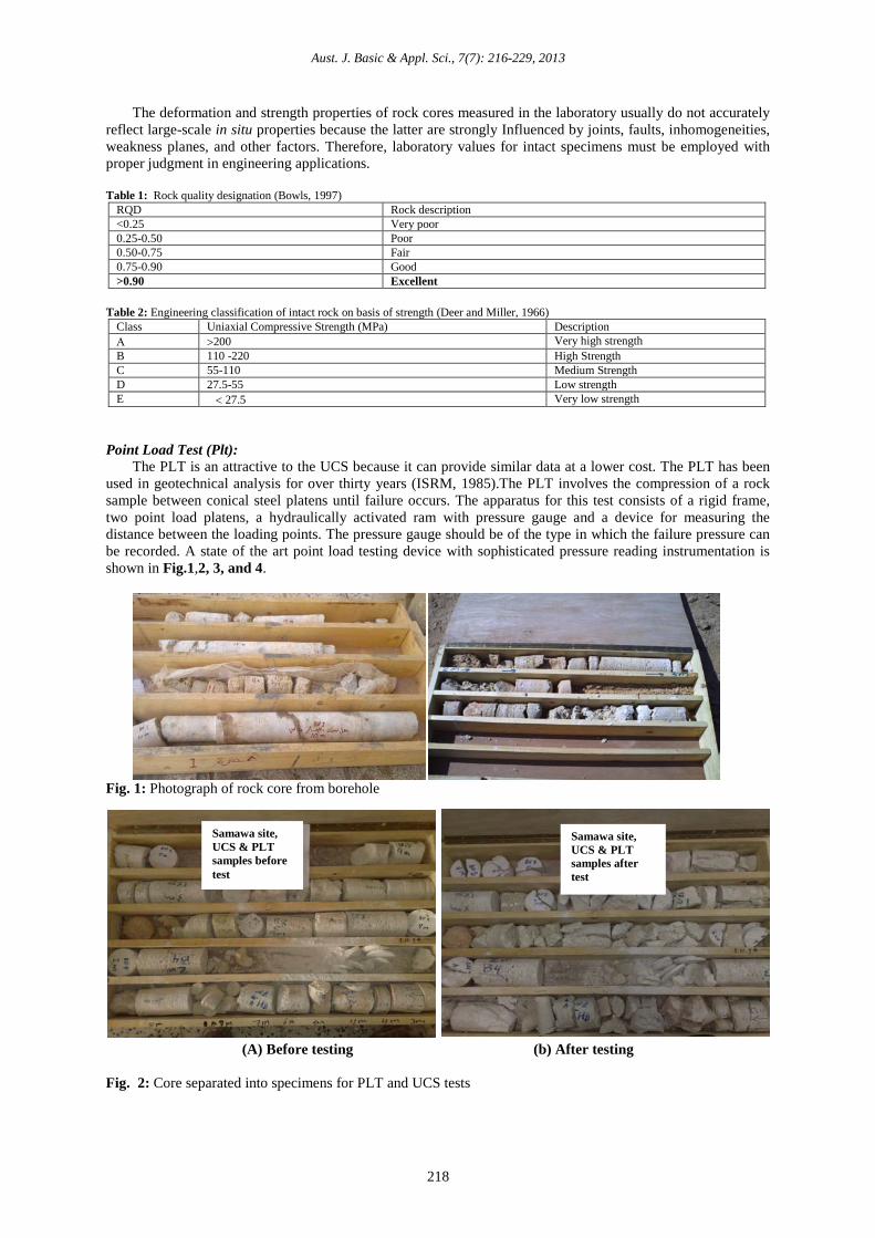
used in geotechnical analysis for over thirty years (ISRM, 1985).The PLT involves the compression of a rock sample between conical steel platens until failure occurs. The apparatus for this test consists of a rigid frame, two point load platens, a hydraulically activated ram with pressure gauge and a device for measuring the distance between the loading points. The pressure gauge should be of the type in which the failure pressure can be recorded. A state of the art point load testing device with sophisticated pressure reading instrumentation is shown in Fig.1,2, 3, and 4.

Fig. 1: Photograph of rock core from borehole

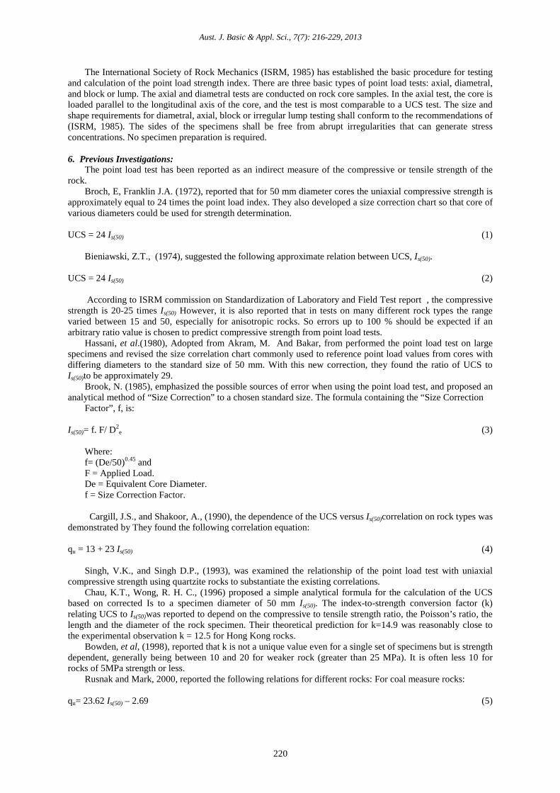
(A) Before testing (b) After testing Fig. 2: Core separated into specimens for PLT and UCS tests

Samawa site, UCS & PLT samples after test

Samawa site, UCS & PLT samples before test


219

(A) Before testing (B) UCS Test Device (C) After testing

Fig. 3: Core specimens for UCS tests.

Fig

Fig. 4: Pictorial overview of PLT stages.

Samawa site, UCS samples before test

Samawa site, UCS samples after test

Samawa site


220

The International Society of Rock Mechanics (ISRM, 1985) has established the basic procedure for testing and calculation of the point load strength index. There are three basic types of point load tests: axial, diametral, and block or lump. The axial and diametral tests are conducted on rock core samples. In the axial test, the core is loaded parallel to the longitudinal axis of the core, and the test is most comparable to a UCS test. The size and shape requirements for diametral, axial, block or irregular lump testing shall conform to the recommendations of (ISRM, 1985). The sides of the specimens shall be free from abrupt irregularities that can generate stress concentrations. No specimen preparation is required.

6. Previous Investigations:

The point load test has been reported as an indirect measure of the compressive or tensile strength of the rock.

Broch, E, Franklin J.A. (1972), reported that for 50 mm diameter cores the uniaxial compressive strength is approximately equal to 24 times the point load index. They also developed a size correction chart so that core of various diameters could be used for strength determination.

UCS = 24 Is(50) (1)

Bieniawski, Z.T., (1974), suggested the following approximate relation between UCS, Is(50).

UCS = 24 Is(50) (2) According to ISRM commission on Standardization of Laboratory and Field Test report , the compressive

strength is 20-25 times Is(50) However, it is also reported that in tests on many different rock types the range varied between 15 and 50, especially for anisotropic rocks. So errors up to 100 % should be expected if an arbitrary ratio value is chosen to predict compressive strength from point load tests.

Hassani, et al.(1980), Adopted from Akram, M. And Bakar, from performed the point load test on large specimens and revised the size correlation chart commonly used to reference point load values from cores with differing diameters to the standard size of 50 mm. With this new correction, they found the ratio of UCS to Is(50)to be approximately 29.

Brook, N. (1985), emphasized the possible sources of error when using the point load test, and proposed an analytical method of “Size Correction” to a chosen standard size. The formula containing the “Size Correction

Factor”, f, is:

Is(50)= f. F/ D2e (3)

Where: f= (De/50)0.45 and F = Applied Load. De = Equivalent Core Diameter. f = Size Correction Factor. Cargill, J.S., and Shakoor, A., (1990), the dependence of the UCS versus Is(50)correlation on rock types was

demonstrated by They found the following correlation equation:

qu = 13 + 23 Is(50) (4) Singh, V.K., and Singh D.P., (1993), was examined the relationship of the point load test with uniaxial

compressive strength using quartzite rocks to substantiate the existing correlations. Chau, K.T., Wong, R. H. C., (1996) proposed a simple analytical formula for the calculation of the UCS

based on corrected Is to a specimen diameter of 50 mm Is(50). The index-to-strength conversion factor (k) relating UCS to Is(50)was reported to depend on the compressive to tensile strength ratio, the Poisson’s ratio, the length and the diameter of the rock specimen. Their theoretical prediction for k=14.9 was reasonably close to the experimental observation k = 12.5 for Hong Kong rocks.

Bowden, et al, (1998), reported that k is not a unique value even for a single set of specimens but is strength dependent, generally being between 10 and 20 for weaker rock (greater than 25 MPa). It is often less 10 for rocks of 5MPa strength or less.

Rusnak and Mark, 2000, reported the following relations for different rocks: For coal measure rocks:

qu= 23.62 Is(50) – 2.69 (5)


221

For other rocks:

qu= 8.41 Is(50)+ 9.51 (6) Akram, M. And Bakar, (2007), performed Two hundred rock cores were drilled and used for the uniaxial

compressive strength and point load index tests. The UCS was found to be correlated with Is(50) through a linear relationship having slope of 22.792 and intercept of 13.295 for Group A rocks. The UCS versus Is (50) correlation for Group B rocks was also found to be linear but with a slope of 11.076 and zero intercept. This study confirms that the UCS estimation equations are rock dependent. Table 3 Shows Published comparisons between the PLT and UCS for sedimentary rock (Rusnak, J. and Mark C., 2000).

Table 3: Published comparisons between the PLT and UCS for sedimentary rock (Rusnak, J. and Mark C., 2000)

Agustawijaya, D.S., (2007), The UCS values were then correlated with the point load strength index values,

which show a good correlation. The conversion factor for soft rocks is found to be about 14, which is about 58% of the conversion factor for hard rocks.

Conclusion:

The PLT is a fabulous method to determine intact rock strength properties from drill core samples. It has become a famous test in geotechnical engineering. Table 4, and 5 Shows test results of the UCS and PLT for the study.

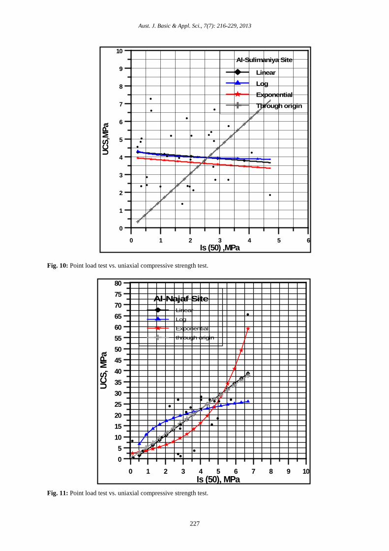
The Iraqi rocks from four locations, Erbil, Al-Samawa, Al- Sulaimaniya, and AL-Najaf sites were used to find the conversion factor k between UCS and PLT. Figs. between 8 and 12 show UCS values were correlated with the point Load strength index values, which show a good correlation using the regression equation of through origin equation which is showing the best coefficient of determination, R-squared.

The conversion factor for Iraqi rocks is found to be about (5.28) for CLAYSTONE ROCK, between (5.65 and 11.18) for LIMESTONE ROCK, and (1.52) for greenish gray SANDSTONE ROCK, which are about (8-40 %) of the conversion factor for hard rocks. The rock type is almost very low strength due to that the average UCS is below 27.5 MPa. This study confirms that the UCS estimation equations are rock dependent.


222

Table 4: Summary of results of the UCS and PLT test for rocked samples

Site Locations Rock Type No. of specimens

Uniaxial Compressive Strength,UCS Point Load Strength Index, Is 50

Mean (MPa)

Standard Deviation

Mean (MPa)

Standard Deviation

(MPa)

Coefficient of Variation

(%)

(MPa)

Coefficient of

Variation (%)

Erbil Site

CLAYSTONE, Reddish Brown

40 20.35

1.485

7.23 2.405 0.253 10.54

Al-Samawa site

LIMESTONE, White

155 13.27 2.92 22.00 1.078 0.419 38.83

Al-Sulaimaniya Site

SANDSTONE, Greenish Gray to Gray

30 4.05 1.612

39.81 1.892 1.170

61.83

Al-Najaf Site

LIMESTONE, White and Milky

23 18.88 13.72

72.64

3.39

1.638 48.33

Table 5: Summary of fit equation results

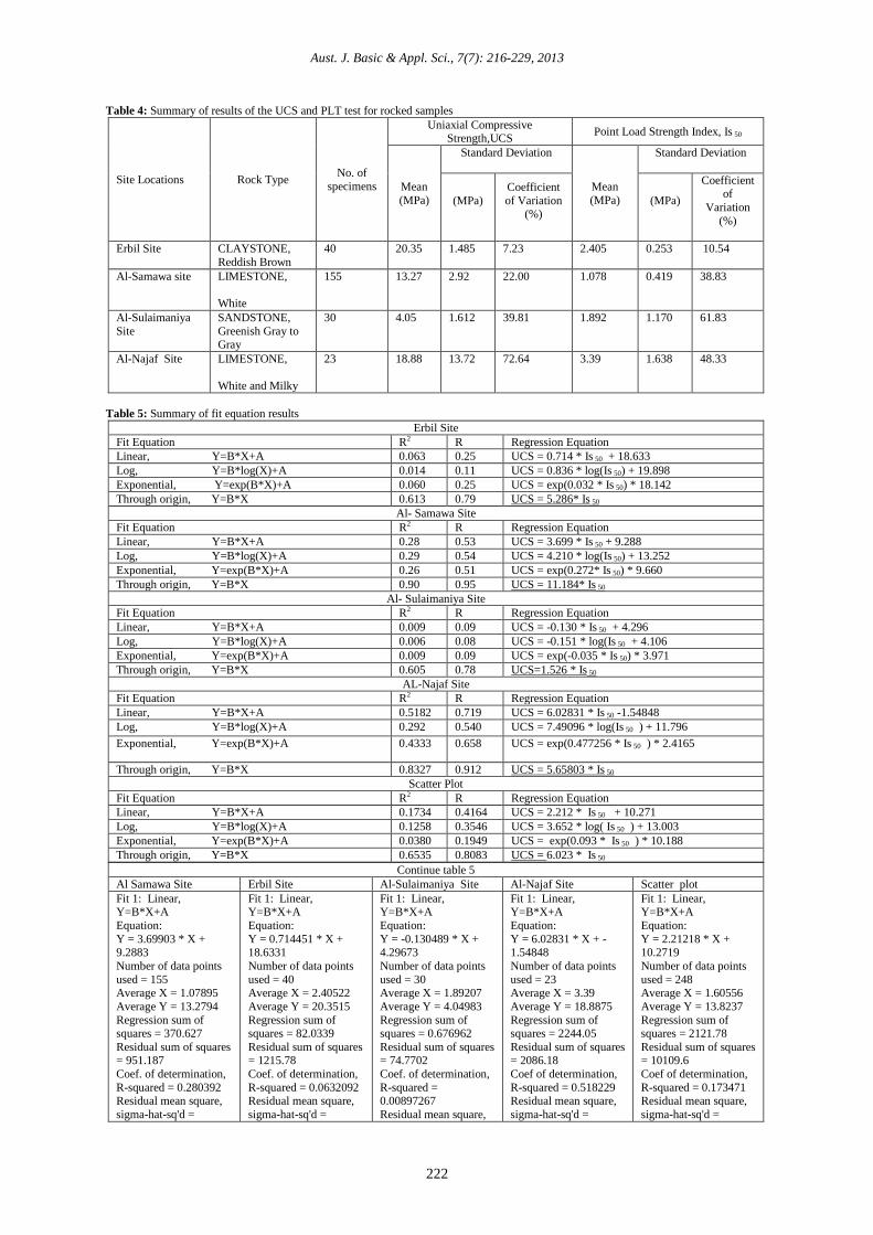
Erbil Site Fit Equation R2 R Regression Equation Linear, Y=B*X+A 0.063 0.25 UCS = 0.714 * Is 50 + 18.633 Log, Y=B*log(X)+A 0.014 0.11 UCS = 0.836 * log(Is 50) + 19.898 Exponential, Y=exp(B*X)+A 0.060 0.25 UCS = exp(0.032 * Is 50) * 18.142 Through origin, Y=B*X 0.613 0.79 UCS = 5.286* Is 50

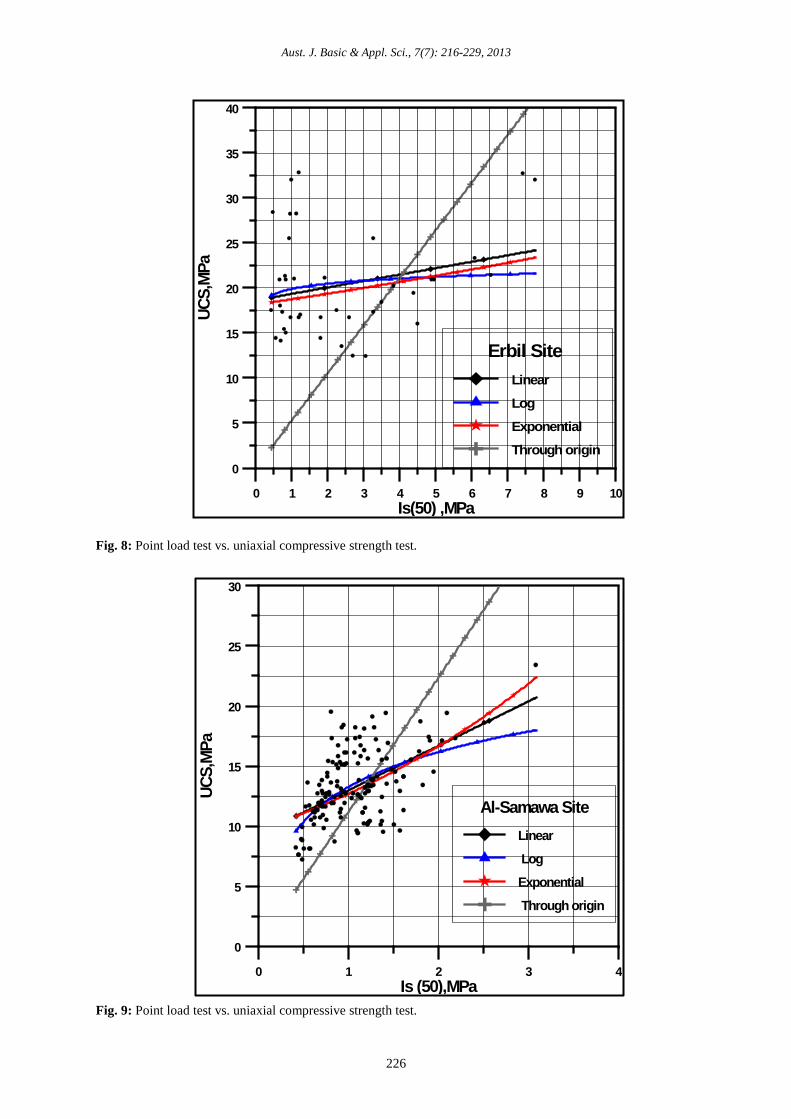
Al- Samawa Site Fit Equation R2 R Regression Equation Linear, Y=B*X+A 0.28 0.53 UCS = 3.699 * Is 50 + 9.288 Log, Y=B*log(X)+A 0.29 0.54 UCS = 4.210 * log(Is 50) + 13.252 Exponential, Y=exp(B*X)+A 0.26 0.51 UCS = exp(0.272* Is 50) * 9.660 Through origin, Y=B*X 0.90 0.95 UCS = 11.184* Is 50

Al- Sulaimaniya Site Fit Equation R2 R Regression Equation Linear, Y=B*X+A 0.009 0.09 UCS = -0.130 * Is 50 + 4.296 Log, Y=B*log(X)+A 0.006 0.08 UCS = -0.151 * log(Is 50 + 4.106 Exponential, Y=exp(B*X)+A 0.009 0.09 UCS = exp(-0.035 * Is 50) * 3.971 Through origin, Y=B*X 0.605 0.78 UCS=1.526 * Is 50

AL-Najaf Site Fit Equation R2 R Regression Equation Linear, Y=B*X+A 0.5182 0.719 UCS = 6.02831 * Is 50 -1.54848 Log, Y=B*log(X)+A 0.292 0.540 UCS = 7.49096 * log(Is 50 ) + 11.796 Exponential, Y=exp(B*X)+A 0.4333 0.658 UCS = exp(0.477256 * Is 50 ) * 2.4165

Through origin, Y=B*X 0.8327 0.912 UCS = 5.65803 * Is 50 Scatter Plot

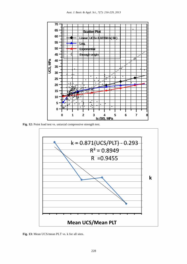
Fit Equation R2 R Regression Equation Linear, Y=B*X+A 0.1734 0.4164 UCS = 2.212 * Is 50 + 10.271 Log, Y=B*log(X)+A 0.1258 0.3546 UCS = 3.652 * log( Is 50 ) + 13.003 Exponential, Y=exp(B*X)+A 0.0380 0.1949 UCS = exp(0.093 * Is 50 ) * 10.188 Through origin, Y=B*X 0.6535 0.8083 UCS = 6.023 * Is 50

Continue table 5 Al Samawa Site Erbil Site Al-Sulaimaniya Site Al-Najaf Site Scatter plot Fit 1: Linear, Y=B*X+A Equation: Y = 3.69903 * X + 9.2883 Number of data points used = 155 Average X = 1.07895 Average Y = 13.2794 Regression sum of squares = 370.627 Residual sum of squares = 951.187 Coef. of determination, R-squared = 0.280392 Residual mean square, sigma-hat-sq'd =

Fit 1: Linear, Y=B*X+A Equation: Y = 0.714451 * X + 18.6331 Number of data points used = 40 Average X = 2.40522 Average Y = 20.3515 Regression sum of squares = 82.0339 Residual sum of squares = 1215.78 Coef. of determination, R-squared = 0.0632092 Residual mean square, sigma-hat-sq'd =

Fit 1: Linear, Y=B*X+A Equation: Y = -0.130489 * X + 4.29673 Number of data points used = 30 Average X = 1.89207 Average Y = 4.04983 Regression sum of squares = 0.676962 Residual sum of squares = 74.7702 Coef. of determination, R-squared = 0.00897267 Residual mean square,

Fit 1: Linear, Y=B*X+A Equation: Y = 6.02831 * X + -1.54848 Number of data points used = 23 Average X = 3.39 Average Y = 18.8875 Regression sum of squares = 2244.05 Residual sum of squares = 2086.18 Coef of determination, R-squared = 0.518229 Residual mean square, sigma-hat-sq'd =

Fit 1: Linear, Y=B*X+A Equation: Y = 2.21218 * X + 10.2719 Number of data points used = 248 Average X = 1.60556 Average Y = 13.8237 Regression sum of squares = 2121.78 Residual sum of squares = 10109.6 Coef of determination, R-squared = 0.173471 Residual mean square, sigma-hat-sq'd =


223

6.21691 31.9943 sigma-hat-sq'd = 2.67036

99.3418 41.0958

Fit 2: Log, Y=B*log(X)+A Equation: Y = 4.21043 * log(X) + 13.2525 Number of data points used = 155 Average log(X) = 0.00637105 Average Y = 13.2794 Regression sum of squares = 382.241 Residual sum of squares = 939.573 Coef. of determination, R-squared = 0.289179 Residual mean square, sigma-hat-sq'd = 6.141

Fit 2: Log, Y=B*log(X)+A Equation: Y = 0.836195 * log(X) + 19.8982 Number of data points used = 40 Average log(X) = 0.542123 Average Y = 20.3515 Regression sum of squares = 18.9391 Residual sum of squares = 1278.88 Coef. of determination, R-squared = 0.0145931 Residual mean square, sigma-hat-sq'd = 33.6546

Fit 2: Log, Y=B*log(X)+A Equation: Y = -0.151456 * log(X) + 4.10647 Number of data points used = 30 Average log(X) = 0.373949 Average Y = 4.04983 Regression sum of squares = 0.459387 Residual sum of squares = 74.9878 Coef .of determination, R-squared = 0.00608886 Residual mean square, sigma-hat-sq'd = 2.67813

Fit 2: Log, Y=B*log(X)+A Equation: Y = 7.49096 * log(X) + 11.7969 Number of data points used = 23 Average log(X) = 0.946553 Average Y = 18.8875 Regression sum of squares = 1268.21 Residual sum of squares = 3062.02 Coef of determination, R-squared = 0.292874 Residual mean square, sigma-hat-sq'd = 145.81

Fit 2: Log, Y=B*log(X)+A Equation: Y = 3.6526 * log(X) + 13.0039 Number of data points used = 248 Average log(X) = 0.224442 Average Y = 13.8237 Regression sum of squares = 1538.89 Residual sum of squares = 10692.5 Coef of determination, R-squared = 0.125815 Residual mean square, sigma-hat-sq'd = 43.4653

Fit 3: Exponential, log(Y)=B*X+A Equation: log(Y) = 0.272233 * X + 2.26809 Alternate equation: Y = exp(0.272233 * X) * 9.6609 Number of data points used = 155 Average X = 1.07895 Average log(Y) = 2.56181 Regression sum of squares = 2.00743 Residual sum of squares = 5.67043 Coef. of determination, R-squared = 0.261458 Residual mean square, sigma-hat-sq'd = 0.0370616

Fit 3: Exponential, log(Y)=B*X+A Equation: log(Y) = 0.0325954 * X + 2.89826 Alternate equation: Y = exp(0.0325954 * X) * 18.1426 Number of data points used = 40 Average X = 2.40522 Average log(Y) = 2.97666 Regression sum of squares = 0.170751 Residual sum of squares = 2.66704 Coef .of determination, R-squared = 0.0601702 Residual mean square, sigma-hat-sq'd = 0.0701854

Fit 3: Exponential, log(Y)=B*X+A Equation: log(Y) = -0.0351647 * X + 1.37918 Alternate equation: Y = exp(-0.0351647 * X) * 3.97166 Number of data points used = 30 Average X = 1.89207 Average log(Y) = 1.31265 Regression sum of squares = 0.0491622 Residual sum of squares = 5.50308 Coef. of determination, R-squared = 0.00885447 Residual mean square, sigma-hat-sq'd = 0.196539

Fit 3: Exponential, log(Y)=B*X+A Equation: log(Y) = 0.477256 * X + 0.882319 Alternate equation: Y = exp(0.477256 * X) * 2.4165 Number of data points used = 23 Average X = 3.39 Average log(Y) = 2.50022 Regression sum of squares = 14.0651 Residual sum of squares = 18.3888 Coef of determination, R-squared = 0.433388 Residual mean square, sigma-hat-sq'd = 0.875657

Fit 3: Exponential, log(Y)=B*X+A Equation: log(Y) = 0.0938488 * X + 2.32122 Alternate equation: Y = exp(0.0938488 * X) * 10.1881 Number of data points used = 248 Average X = 1.60556 Average log(Y) = 2.4719 Regression sum of squares = 3.81871 Residual sum of squares = 96.4818 Coef of determination, R-squared = 0.0380727 Residual mean square, sigma-hat-sq'd = 0.392203

Fit 4: Y=B*X, through origin Equation: Y = 11.1841 * X Number of data points used = 155 Average X = 1.07895 Average Y = 13.2794 Residual sum of squares = 2696.57 Coef. of determination, R-squared = 0.905894 Residual mean square, sigma-hat-sq'd = 17.5102



Fit 4: Y=B*X, through origin Equation: Y = 5.65803 * X Number of data points used = 23 Average X = 3.39 Average Y = 18.8875 Residual sum of squares = 2096.62 Coef of determination, R-squared = 0.832741 Residual mean square, sigma-hat-sq'd = 95.301

Fit 4: Y=B*X, through origin Equation: Y = 6.02358 * X Number of data points used = 247 Average X = 1.61155 Average Y = 13.8471 Residual sum of squares = 20631.2 Coef of determination, R-squared = 0.653596 Residual mean square, sigma-hat-sq'd = 83.8665


224

Fig. 5: PLT VS UCS For previous study (Fener, et al, 2005)

Fig. 6: UCS test curve


225

Fig. 7: Typical soil -rock borehole logs for the studied sites


226

0 1 2 3 4Is (50),MPa

0

5

10

15

20

25

30

UCS,

MPa

Al-Samawa SiteLinear

Log

Exponential

Through origin

Fig. 8: Point load test vs. uniaxial compressive strength test.


0 1 2 3 4 5 6 7 8 9 10Is(50) ,MPa

0

5

10

15

20

25

30

35

40

UCS,

MPa

Erbil Site Linear

Log

Exponential

Through origin


227

0 1 2 3 4 5 6 7 8 9 10Is (50), MPa

05

101520253035404550556065707580

UCS,

MPa

Al-Najaf SiteLinear

Log

Exponential

through origin



0 1 2 3 4 5 6Is (50) ,MPa

0

1

2

3

4

5

6

7

8

9

10

UCS,

MPa

Al-Sulimaniya Site

Linear

Log

Exponential

Through origin


228

0 1 2 3 4 5 6 7 8Is (50), MPa

0

5

10

15

20

25

30

35

40

45

50

55

60

65

70

UCS,

MPa

Scatter Plot

Linear UCS= 6.02358 Is( 50 )

Log,

Exponential

through origin

k = 0.871(UCS/PLT) - 0.293R² = 0.8949R =0.9455

k

Mean UCS/Mean PLT


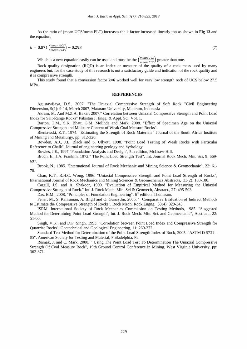
Fig. 13: Mean UCS/mean PLT vs. k for all sites.


229

As the ratio of (mean UCS/mean PLT) increases the k factor increased linearly too as shown in Fig 13.and the equation,

(7)

Which is a new equation easily can be used and must be the greater than one. Rock quality designation (RQD) is an index or measure of the quality of a rock mass used by many

engineers but, for the case study of this research is not a satisfactory guide and indication of the rock quality and it is compressive strength.

This study found that a conversion factor k=6 worked well for very low strength rock of UCS below 27.5 MPa.

REFFERENCES

Agustawijaya, D.S., 2007. "The Uniaxial Compressive Strength of Soft Rock "Civil Engineering

Dimension, 9(1): 9-14, March 2007, Mataram University, Mataram, Indonesia Akram, M. And M.Z.A. Bakar, 2007." Correlation between Uniaxial Compressive Strength and Point Load

Index for Salt-Range Rocks" Pakistan J. Engg. & Appl. Sci. Vol. 1. Barton, T.M., S.K. Bhatt, G.M. Molinda and Mark, 2008. "Effect of Specimen Age on the Uniaxial

Compressive Strength and Moisture Content of Weak Coal Measure Rocks". Bieniawski, Z.T., 1974. "Estimating the Strength of Rock Materials" Journal of the South Africa Institute

of Mining and Metallurgy, pp: 312-320. Bowden, A.J., J.L. Black and S. Ullyott, 1998. "Point Load Testing of Weak Rocks with Particular

Reference to Chalk", Journal of engineering geology and hydrology. Bowles, J.E., 1997."Foundation Analysis and Design", 5th edition, McGraw-Hill. Broch, E., J.A. Franklin, 1972." The Point Load Strength Test". Int. Journal Rock Mech. Min. Sci, 9: 669-

697. Brook, N., 1985. "International Journal of Rock Mechanic and Mining Science & Geomechanic", 22: 61-

70. Chau, K.T., R.H.C. Wong, 1996. "Uniaxial Compressive Strength and Point Load Strength of Rocks",

International Journal of Rock Mechanics and Mining Sciences & Geomechanics Abstracts, 33(2): 183-188. Cargill, J.S. and A. Shakoor, 1990. "Evaluation of Empirical Method for Measuring the Uniaxial

Compressive Strength of Rock." Int. J. Rock Mech. Min. Sci & Geomech, Abstract., 27: 495-503. Das, B.M., 2008. "Principles of Foundation Engineering", 6th edition, Thomason. Fener, M., S. Kahraman, A. Bilgil and O. Gunaydin, 2005. " Comparative Evaluation of Indirect Methods

to Estimate the Compressive Strength of Rocks", Rock Mech. Rock Engng, 38(4): 329-343. ISRM. International Society of Rock Mechanics Commission on Testing Methods, 1985. "Suggested

Method for Determining Point Load Strength", Int. J. Rock Mech. Min. Sci. and Geomechanic", Abstract., 22: 51-60.

Singh, V.K., and D.P. Singh, 1993. "Correlation between Point Load Index and Compressive Strength for Quartzite Rocks", Geotechnical and Geological Engineering, 11: 269-272.

Standard Test Method for Determination of the Point Load Strength Index of Rock, 2005. "ASTM D 5731 – 05", American Society for Testing and Material, Philadelphia, Pa.

Rusnak, J. and C. Mark, 2000. " Using The Point Load Test To Determination The Uniaxial Compressive Strength Of Coal Measure Rock", 19th Ground Control Conference in Mining, West Virginia University, pp: 362-371.

http://academic.research.microsoft.com/Publication/27371649/uniaxial-compressive-strength-and-point-load-strength-of-rocks�

http://academic.research.microsoft.com/Journal/14062/international-journal-of-rock-mechanics-and-mining-sciences-&-geomechanics-abstracts�

correlation between point load index and very low...

Documents