C O R R O S I O N BEHAVIOR OF X70 PIPELINE STEEL IN H2S C O N T A I N I N G S O L U T I O N S

Sergio Arzola-Peralta*, Juan Genesca-Llongueras*, Juan Mendoza-Flores**, Ruben Duran-Romero**

Dpto. Ingenieria Metalflrgica. Facultad Quimica. Universidad Nacional Autdnoma M6xico (UNAM).

Ciudad Universitaria. 04510 Mdxico D.F.

Direcci6n Ejecutiva de Exploraci6n y Producci6n. Corrosidn.

Instituto Mexicano del Petrdleo Eje Central L. Cfirdenas # 152

07730 M6xico D.F.

ABSTRACT

The present work describes the corrosion behavior of X70 pipeline steel immersed in H2S solutions. Electrochemical techniques such as Linear Polarization Resistance (LPR), Electrochemical Impedance Spectroscopy, EIS and Electrochemical Noise, EN, were used to characterize the electrochemical behavior of X70 pipeline steel in a 3 wt% NaC1 solution with several hydrogen sulfide (H2S) concentrations; 0, 100, 650 an 2550 ppm. Electrochemical Noise Measurements, ENM, have been carried out on this system in order to identify the type of corrosion. Electrochemical parameters like, Polarization Resistance, Re, corrosion rate, CR and Noise Resistance, Rn are presented. Additionally, a comparison of corrosion rate values between static and turbulent flow conditions was made. To simulate flow conditions, the rotating cylinder electrode, RCE, in turbulent flow regime (1000 rprn) for a saturated H2S solution was used.

Keywords Pipeline steel, H2S, Electrochemical Noise, turbulent flow.

INTRODUCTION

The study of corrosion behavior of X70 pipeline steel has been presented recently 1 using EIS technique. In this work a mixed control (charge-transfer and diffusion) was determined by means of the analysis of electrochemical impedance spectra. At high frequencies a transfer process takes place while at low frequencies (0.01-0.001 Hz) a diffusion process was characterized by the presence of a Warburg

impedance. The goal of present work is to study the corrosion behavior of the X70 pipeline steel in terms of the time series recorded in the free corrosion potential of steel in H2S containing solutions. Many authors have studied 2-7 the corrosion of steel and iron in H2S containing solutions, however, the use of Electrochemical Noise Measurements ENM, has been quite limited. Dvoracek 8 has found that the pitting of steel in H2S solutions may take place between pH values of 3 and 6 in a NaC1 solution (355 ppm of CI) saturated with H2S at room temperature. The iron sulfide film formation on steel surface it is well documented 9-14. Most of these researchers have pointed out that this film is non-protective because of the high corrosion values measured in several study conditions, some others a5 suggested that under particular circumstances the iron sulfide film might be protective. The phases that develops through this film are reported 3 to be mackinawite FeSl.x, followed by cubic FeS and troilite (hexagonal FeS), pyrrhotite and pyrite, FeS2, depending on experimental study conditions. Shoesmith reported 16 the formation of three iron monosulfide phases as a function of time, pH and applied current: mackinawite FeSl_x, cubic ferrous sulfide and troilite Therefore, ENM will provide information about the iron sulfide film behavior and the corrosion mechanism of X70 pipeline steel in H2S solutions.

EXPERIMENTAL

Electrodes and electrolytes

The working electrode was made of a cylindrical steel X-70 bar, 1.105 cm (0.435 inches) of diameter and 0.851 cm (0.335 inches) of height. The counter electrode was a rod of sintered graphite, while a saturated calomel electrode (SCE), was the reference electrode. The steel surface was polished with 600 grit SiC paper then was cleaned and degreased with acetone and finally washed with distilled water. Four deareated solutions were studied: a 3 wt% NaC1 solution with 0, 100, 650 and 2550 ppm of H2S with 6.94, 5.34, 4.38 and 4.11 pH values respectively. In order to eliminate the dissolved oxygen, all solutions were purged with N2 before each test, subsequently they were bubbled with H2S. For the lower concentrations of H2S an aliquot was taken from an already saturated solution to prepare the concentrations of both 650 and 100 ppm. All experiments were performed at atmospheric pressure (Mexico City) and at two different temperatures, 20 and 60°C.

Apparatus

All electrochemical experiments were carried out with a Solartron 1280B Electrochemical Measurement unit controlled by Corrware and Zplot Software. For all the techniques studied here, the conventional three-electrode system was used. For ENM, two-identical samples were used. The sampling time was 1 second/point, taking a total of 2058 points. EIS was measured from an initial frequency of 10 KHz to a final frequency of 0.001 Hz with an amplitude of 10 mV from the corrosion potential. The rotating cylinder electrode, RCE, Perkin-Elmer EG&G Model 636 was used to simulate turbulent flow conditions at 1000 rpm (Reynolds number ~ 6900) for the H2S saturated solution. An electrochemical monitoring of 24 hours was carried out for all the conditions, open circuit potential, OCP, Linear Polarization Resistance, LPR, Electrochemical Impedance Spectroscopy, EIS, formed one hour cycle and ENM were measured separately in a different 24 hours monitoring taking 2058 point each hour.

EXPERIMENTAL RESULTS AND DISCUSSION

The study of X70 pipeline steel in three different H2S containing solutions have been recently presented 1. The Nyquist diagrams (Figure 1) show the general behavior of steel as a function of H2S

concentration. For the three H2S conditions, Nyquist plot is formed by two processes, frequencies the iron dissolution take place and at low frequencies diffusion is present.

12000

10000

8000 E o

6000

E - - 4000

I

2000

i

A % ¢J

1:11

E

1000

800

600

400

200

0 5 0 0 0 10000 1 5 0 0 0 0

Real I m p e d a n c e (f~.cm 2)

i i i

500 1000 1500 2000

R e a l I m p e d a n c e (f2 . cm 2)

a) b)

350 250

300

,,,-,, 250

E 200

150 E ' 100

50

200

E ca 150

100 E , i i

!

50

w i i | u ~ i i i

0 250 500 750 1000 0 200 400 600 800

Real Impedancd (f2.cm 2) Real Impedance (f~.cm 2)

at high

c) d)

FIGURE 1. Nyquist impedance spectra of X70 steel immersed in: (a) 3 wt% NaC1 solution with different H2S concentration: (b) 100ppm, (c) 650ppm and (d) 2550ppm, at zero (o) and 24 hours of

exposure (.).

These plots made clear the formation of a corrosion product on steel surface reported previously by several authors as mackinawite, which take place at low frequencies range (between 0.01 and 0.001 Hz). In solutions containing H2S, carbon steel corrodes. The corrosion process is generally accompanied by the formation of sulfide film. As can be seen in Figure lb, in the 3wt% NaC1 solution with 100 ppm H2S and at the initial time, the presence of H2S reduced the diameter of the semicircle in the Nyquist plot about 19 times from that diameter observed in Figure l a. This fact confirms that the presence of HgS produces an increase in the corrosion rate of steel. By effect of immersion time, the diameter of the high- frequency semicircle increases, which can be ascribed to the growth of a sulfide film, improving its corrosion resistance. In a solution containing H2S, the H2S concentration plays an important role in determining the characteristics of the sulfide on carbon steel. By increasing the H2S concentration, the same effect can be observed independently of H2S concentration. Figures l c and l d show the

impedance spectra of X70 steel in the 3wt% NaC1 solution with 650 and 2550 ppm of H2S, respectively. These two plots seem to be equivalent, except for the difference between their ect values. Rct corresponds to the diameter of high-frequency semicircle.

Electrochemical noise

Time series of X70 pipeline steel immersed in H2S containing solutions are shown in Figure 2. Electrochemical potential and current fluctuations were simultaneously measured. It is possible to note from this Figure that there are positive and negative current transients in the 100 ppm of H2S solution at 20°C. According to Cottis and Turgoose 17 this behavior is characteristic of pitting events on X70 steel surface. However, in this study, there is not physical evidence of any pitting looking at the SEM photography of steel surface (see Figure l 0), which shows the typical scale formed on steel surface after 24 hours of exposure in the H2S saturated solution.

1 . 0 0 E - 0 6

O.OOE+O0 - A

~,~ - 1 . 0 0 E - 0 6

,~, - 2 . 0 0 E - 0 6 - c

L _ L _

0

- 3 . 0 0 E - 0 6 -

- 4 . 0 0 E - 0 6 -

-5. OOE-06 -

-6. OOE-06

0 500 1000 1500 2 0 0 0

time (s)

a)

1 . 0 0 E - 0 5

._.. 5 0 0 E - 0 6 B

,,,-, 0 . 0 0 E + 0 0 i,,,,,

' - - 5 . 0 0 E - 0 6

O - 1 . 0 0 E - 0 5

- 1 . 5 0 E - 0 5

0 5 0 0 1 0 0 0 1 5 0 0 2 0 0 0

t i m e ( s )

b) FIGURE 2. Current and potential time series for the X70 steel in the sodium chloride electrolyte with 100 ppm of H2S at 20 a) and 60°C. One point/second. At 1.30 h (A), 12 h (B) and 24 h (C) of exposure time.

In the other hand, the very high corrosion values calculated for the H2S conditions show that the film formed on steel surface cannot passivate the metal at any level. Therefore, because there is not a "passive film" it cannot be any development of pitting, like in the typical cases of steel in an alkaline solution with CI or stainless steel in a NaC1 solution. Similar behavior can be observed in the 2550 ppm of H2S solution at 20°C. Apparently transients of pitting have been developed, however, no characteristic frequencies are present in the PSD plot for all studied conditions (see Figures 4 through 7).

4.00E-06

3 0 0 E - 0 6

~ 2.00E-06 -

1 0 0 E - 0 6 -

'--- O.OOE+O0

0 -1 .00E-06 - ' - ' -~

- 2 0 0 E - 0 6

-3 .00E-06

0 500 1000 1500 2000

t ime (s}

a)

A <

c I,,,,,

¢.,3

8.00E-06

4. OOE-06 ]

O. OOE+O0

-4. OOE-06

-8.00E-06

-1.20E-05 , ,

0 500 1000 1500 2000

t ime (s)

b)

FIGURE 3. NaC1 solution with 2550 ppm of H2S at 20°C a) and b) 60°C. 1.30 h (A), 12 h (B) and 24 h (C) of exposure time. One point/s.

For the time series shown above the PSD were calculated, as well as the slope of the spectra. Table 1 summarizes the slopes calculated for all studied conditions. As it can be seen from this Table the effect of temperature was an increment in the slope value for both H2S concentrations 100 and 2550 ppm.

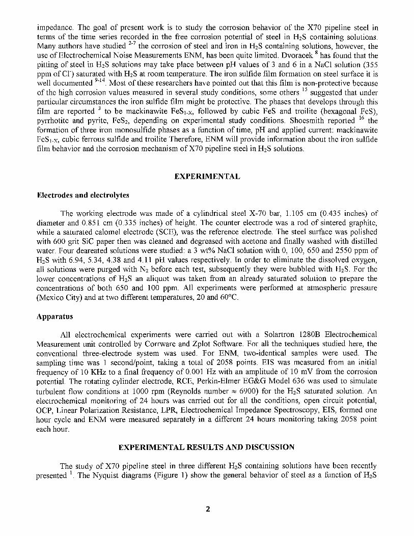
Some authors ~8-~9 have proposed the use of PSD slopes in terms of dB/decade to differentiate between several types of corrosion. According to this fact and for all experimental conditions analyzed here, the uniform corrosion type was the only corrosion type identified; therefore, the presence of pitting is ruled out.

1E-12

1E_111 / ~ 1E-12 1E-13

F ~ 1E-13 1E-14 1E-12 ~ 1E-14

1E-14 , . l~kl ~" 1E-15 "< 1E-16

' 1E-17 1E-15 ] ' " '1 'l ~ 1E-17 n

n 1 E - 1 6 ~ Q" 1E-18 1E-18

1 E - 1 7 ~ 1E-19 1E-19

1E'lS-d . . . . . . . . . . . . . . . . . . . . . . . . 1E-20 . . . . . . 1E-20 . . . . 1'i~-~ ool ol i / Z 3 . . . . . . o 5 1 o:1 . . . . "1 ' /~-3 . . . . . . & l . . . . . . '611

Frequency (Hz) Frequency (Hz) Frequency (Hz)

1E-11

1E-12

1E-13

'r- 1E-14 -< £3 1E-15 (,9 n 1E-16

1E-17

1E-18

b) a) 1E-10.

1E-11

1E-12

"~" 1E-13-

1E-14.

1E-15 13_

1E-16

1E-17

. . . . . . 0'.[)1 . . . . . . Oil . . . .

Frequency (Hz)

'i~-3 " 1 ' ~ - 3 . . . . . . o i ; 1 . . . . . . . o:1 . . . . . . 1 '~-3 . . . . . . ; ' . ; 1 . . . . . . o :1

Frequency (Hz) Frequency (Hz)

c) 1E-10 ~ ~ ~ / )

1E-11

1E-12

,"~" 1E-14

a 1E-15 03 a.. 1E-16

1E-17

1E-18 . . . .

d ) e) f)

FIGURE 4. Current PSD plots for the X70 steel in the 3 % NaC1 solution with 100 ppm H2S, at 20°C, a) 0 h, b) 12 h, c) 24 h and 60°C, d) 0 h, e) 12 h, f) 24 h.

1E-11

1E-12

1E-13

1E-14 ~,, -r 1E-15

1E-16 £3 cO 1E-17 13.

1E-18

1E-19

1E-121

1E-13

1E-14

,~, 1E-15

<:( 1E-17

1E-18

1E-19

1 E-20

1 E-21

'1'/~-3 . . . . . . o 5 1 . . . . . . o11

Frequency (Hz)

"1i~-3 . . . . . . o:;1 . . . . . . o:1 . . . .

Frequency (Hz)

1E-12

1E-13

1E-14

1E-15 O n ~ 1E-16

1E-17

1E-18

1E-3 0.01 0.1

Frequency (Hz)

a) b) c)

1E-11

1E-12

1E-13

~<.~ 1 E-14 D 03 a_ 1E-15

1E-16

1E-3

1E-11

1E-12

1E-13

1E-14

~<~ 1E-15

a 1E-16 o3 n 1E-17

1E-18

1E-19

1E-9

1E-10

1E-11

1E-12.

~" 1 E-13. "1" 1E-14.

,,_., C3 1E-15. 69 n 1E-16.

1E-17.

1E-18.

'4~-3 . . . . . . &l . . . . . . o 1 1 . . . .

Frequency (Hz)

e)

0.01 0.1 1E-3 0.01 0.1

Frequency (Hz) Frequency (Hz)

d) 0

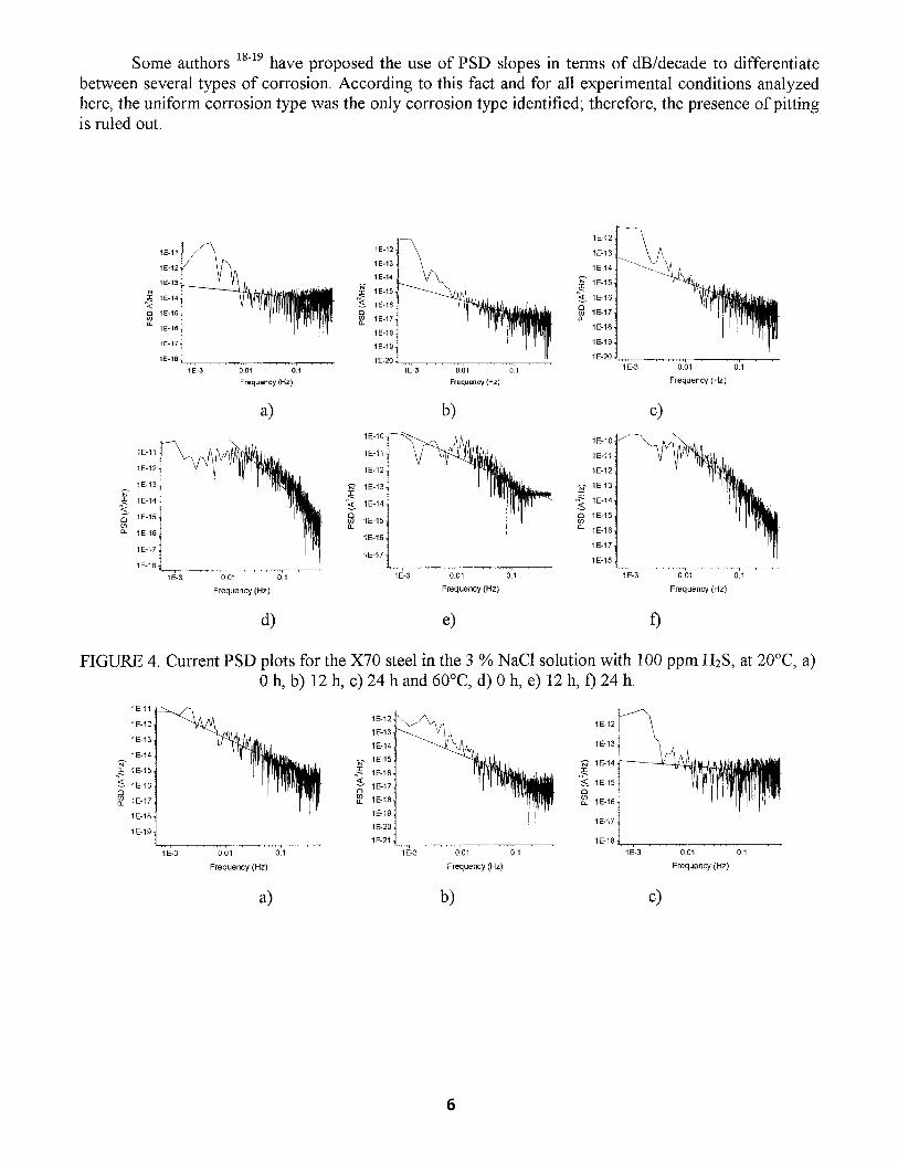
FIGURE 5. Current PSD plots for the X70 steel in the 3 % NaC1 solution with 2550 ppm H2S at 20°C, a) 0 h, b)12 h, c) 24 h and 60°C, d) 0 h. e)12 h, f) 24 h

Table 1. PSD slopes for 100 and 2550 ppm of H2S.

Concentration (H2S)

1 O0 ppm 2550 ppm 100 ppm

2550 ppm

Temperature, °C

20 20 60 60

Slope db/decade

-0.341,-1.007,-1.335 -1.732, -1.607, -0.222 -2.956. -1.466, -3.186 -1.007, -2.929, -3.452

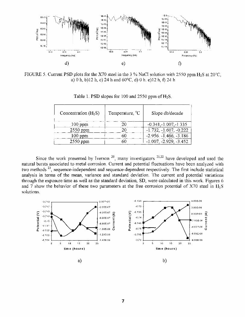
Since the work presented by Iverson 20, many investigators 21,22 have developed and used the natural bursts associated to metal corrosion. Current and potential fluctuations have been analyzed with two methods 23, sequence-independent and sequence-dependent respectively. The first include statistical analysis in terms of the mean, variance and standard deviation. The current and potential variations through the exposure time as well as the standard deviation, SD, were calculated in this work. Figures 6 and 7 show the behavior of these two parameters at the free corrosion potential of X70 steel in H2S solutions.

- 0 . 7 4 6

- 0 . 7 4 7

. - . - 0 . 7 4 8 > " - " - 0 . 7 4 9

t~ - 0 . 75

-0 .751 O

n - 0 . 7 5 2

- 0 . 7 5 3

- 0 . 7 5 4

0 .00 E+00 - 0 . 7 2 5

- 2 .00 E-07 - 0 . 73

- 4 . 0 0 E - 0 7 ,~ > - 0 . 7 3 5

- 6 . 0 0 E - 0 7 ~ "~ -0 .74

¢" - 0 . 7 4 5 - 8 . 0 0 E - 0 7 ' -

- I O -0 .75 - 1 . 0 0 E - 0 6 t~ 12.

- 1 .20 E-06 - 0 . 7 5 5

- 1 . 4 0 E - 0 6 -0 .76

4 . 0 0 E - 0 6

2 . 0 0 E - 0 6

A 0 . 0 0 E + O 0

,,._..

,+.,

e- > - 2 . 0 0 E - 0 6 tla

L_ I .

- 4 . 0 0 E - 0 6 "~ O

- 6 . 0 0 E - 0 6

- 8 . 0 0 E - 0 6

10 15

t i m e ( h o u r s )

2 0 2 5 10 15

t i m e ( h o u r s )

2 0 2 5

a) b)

- 0 . 7 1 8

-0 .72

,_., - 0 .722 > " - " - 0 . 7 2 4

t~ - 0 . 7 2 6 e-

ll; - 0 . 7 2 8

O I~. -0 .73

-0 .732

- 0 . 7 3 4

4 . 0 0 5 - 0 6 - 0 . 7 1 2

- 0 . 7 1 4 2 . 0 0 E - 0 6

- 0 . 7 1 6

0 .00E+00 ~1~ > - 0 . 7 1 8

- 0 . 7 2

- 2 . 0 0 E - 0 6 ~- ' ~ ,_ I::: - 0 . 7 2 2

- 4 . 0 0 E - 0 6 ~ "~ O - 0 . 7 2 4 tO 0 ,

- 0 . 7 2 6 - 6 . 0 0 E - 0 6

- 0 . 7 2 8

- 8 . 0 0 E - 0 6 -0 .73

0 5 10 15 20 25 0 5 10 15 20 25

t ime ( h o u r s ) t ime ( h o u r s )

5 . 0 0 5 - 0 7

0 .00E+00 , . - . .

-5 .00 E-07 " - "

Q; I ,

- 1 . 0 0 5 - 0 6 ,_

¢O

-1 .50 E-06

- 2 . 0 0 E - 0 6 ,

c) d)

FIGURE 6. Potential and current variation (mean values) vs. exposure time of X70 steel in the H2S solutions with 100 ppm H2S a) 20°C, b) 60°C, and with 2550 ppm c) 20°C and d) 60°C.

The analysis of these parameters has been proposed to study the corrosion behavior of several systems 21,22. In Figure 6, the potential variation trends tend to increase its value through the 24 hrs monitoring. In the other hand, current trend was almost always to reduce its mean value, which is in good agreement with the changes in corrosion values. The same analysis for the SD of current and potential show that the potential SD is changing its value continuously and for the fifteen hours (approximately) the SD reaches a maximum, Figure 7.

1 . 3 6 E - 0 3 3.00 E-07

1.34 E-03

e- 1.32 E-03 Q;

O I~. 1.30 E-03

13 If; 1.28 E-03

1.26 E-03

1.27 E-03

lO

t ime (s)

1.34 E-03

2 . 5 0 E - 0 7 1.33 E-03

~ " ,.-., 1 . 3 2 5 - 0 3 2 . 0 0 E - 0 7 ~ "~

Q; .-- 1.31 E-03

1.50 E-07 ~ 1.30 E-03

,._., 0 1.29 E-03 1 . 0 0 E - 0 7 a 0 .

" " 1 . 2 8 5 - 0 3

5.00 E-08 t,t; 1.27 E-03

1.26 E-03 0.00 E+00

1.25 E-03

2 0 0 5 10 15 20

tim e (s)

1.40 E-06

1.20 E-06

,,.--.,,

1.00 E-06

8 . 0 0 E - 0 7 "-- L

6.00 E-07 t~

4.00 E-07 a

2 . 0 0 E - 0 7

0 .00E+00

1.27 E-03

" " 1 . 2 6 E - 0 3 m

, - 1.26 E-03

e- 1.25 E-03 Q;

O 1.25 E-03 I%. ---, 1 . 2 4 E - 0 3 a

1.24 E-03

1.23 E-03

1.23 E-03 0.00 E+00

a)

2 . 5 0 E - 0 7 1 . 3 4 E - 0 3

1 . 3 2 E - 0 3

2 . 0 0 5 - 0 7

e-, ~ 1 . 3 0 E - 0 3

1.50 E-07 Q; ~' ~ 1 . 2 8 E - 0 3

'~ O 1 . 0 0 E - 0 7 tO a .

,,-,, " - " 1 . 2 6 E - 0 3 13 13

5 . 0 0 5 - 0 8 ~ ~ 1 . 2 4 E - 0 3

1 . 2 2 E - 0 3

5 10 15 20 25 0 5 10 15 20 25 0

b)

t i m e ( s ) t i m e ( s )

1 . 2 0 E - 0 6

1 . 0 0 E - 0 6

8 . 0 0 E - 0 7 e"

L. L

6 . 0 0 E ' 0 7 :~

(.,1

4 . 0 0 E - 0 7 ~"

2.00E-07

0 . 0 0 E + 0 0

c) d) FIGURE 7. Potential and current variation (standard deviation, SD ) vs. time exposure of X70 steel in

the H2S solutions with 100 ppm H2S a) 20°C, b) 60°C, and with 2550 ppm: c) 20°C and d) 60°C.

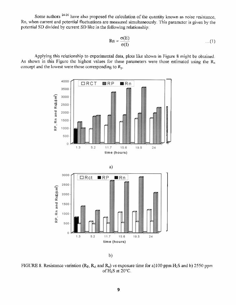
Some authors 24-26 have also proposed the calculation of the quantity known as noise resistance, Rn, when current and potential fluctuations are measured simultaneously. This parameter is given by the potential SD divided by current SD like in the following relationship

o ( E ) R n - . . . ( 1 )

o(I)

Applying this relationship to experimental data, plots like shown in Figure 8 might be obtained. As shown in this Figure the highest values for these parameters were those estimated using the Rn concept and the lowest were those corresponding to Rp.

A "E o

rv

e-

r, n¢

1.3 5.2 24 19.5 11.7 15.6

t i m e ( h o u r s )

4000

3500

3000

2500

2000

1500

1000

500

0

1.3 5.2

a)

3000 1 Rn ] 2500

2000

1500

1000

500

0 19.5 24 11.~ 15.6

t i m e ( h o u r s )

A

4~

tV'

C

t~

b)

FIGURE 8. Resistance variation (Rp, Rct and Rn) vs exposure time for a)100 ppm H2S and b) 25 50 ppm of H2S at 20°C.

Turbulent flow condition

To simulate turbulent flow conditions, the rotating cylinder electrode, RCE was used. As reported by Gabe et al. 27 and Holser et al. 28, this device provides a uniform current distribution as well as a velocity profile with clear defined hydrodynamics. The rotation speed value of RCE was selected as 1000 rpm (Re ~ 6900). Under the study conditions described on experimental procedure, the Reynolds number calculated in this work was as follows:

Re = Vd° ... (2)

where Re = Reynolds number V - Peripheral Velocity (cm/s) do - Cylinder diameter (cm) v - Kinematic fluid viscosity (cm2/s)

Substituting on equation (1): Re = 6897.0057 ~ 6900.

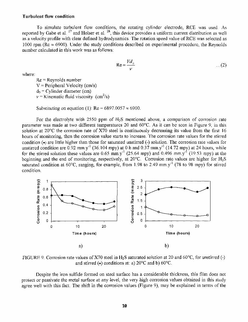
For the electrolyte with 2550 ppm of H2S mentioned above, a comparison of corrosion rate parameter was made at two different temperatures 20 and 60°C. As it can be seen in Figure 9, in this solution at 20°C the corrosion rate of X70 steel is continuously decreasing its value from the first 16 hours of monitoring, then the corrosion value starts to increase. The corrosion rate values for the stirred condition (-) are little higher than those for saturated unstirred (o) solution. The corrosion rate values for unstirred condition are 0.92 mm.y 1 (36.104 mpy) at 0 h and 0.37 mm.y 1 (14.72 mpy) at 24 hours, while for the stirred solution these values are 0.65 mm.y 1 (25.64 mpy) and 0.496 mm.y 1 (19.53 mpy) at the beginning and the end of monitoring, respectively, at 20°C. Corrosion rate values are higher for H2S saturated condition at 60°C, ranging, for example, from 1.98 to 2.49 mm.y 1 (78 to 98 mpy) for stirred condition.

0.8

0.6

0.4

'~o 0.2

o 0 t3

3

E 2.5

.e., e 2

'~o 0 5

o 0 O

0 10 20 0 10 20

T ime (hours) Time (hours)

a) b)

FIGURE 9. Corrosion rate values of X70 steel in H2S saturated solution at 20 and 60°C, for unstirred (o) and stirred (.) conditions at: a) 20°C and b) 60°C.

Despite the iron sulfide formed on steel surface has a considerable thickness, this film does not protect or passivate the metal surface at any level, the very high corrosion values obtained in this study agree well with this fact. The shift in the corrosion values (Figure 9), may be explained in terms of the

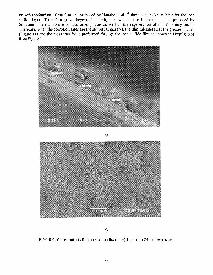
growth mechanism of the film. As proposed by Hausler et al. 29 there is a thickness limit for the iron sulfide layer. If the film grows beyond that limit, then will start to break up and, as proposed by Shoesmith 4 a transformation into other phases as well as the regeneration of this film may occur. Therefore, when the corrosion rates are the slowest (Figure 9), the film thickness has the greatest values (Figure 11) and the mass transfer is performed through the iron sulfide film as shown in Nyquist plot from Figure 1.

::::::::::::::::::::::::::::::::::::::::::::::::::::::::::::::::::::::::::::::::::::::::::::::::::::::::::::.:::::~::::::::::::::::::::::::::::::::::::::::.:::::::::::::::::::::::::::::::.:::::::::::::::::::::::::::::::

,..,..,........,..,...,..,..,.,,-.......-...-.-,-.-.,..,.,,....,......,,.,,. • - • - . • • - . , . . . . , . . . , , . . • • . . . . , . , , . . . , . . , . . . . . . • -..,.,.,,.,.,.,.-.,.,..,.......,.,......,,., - . - . . - . . . . . , , . , , . . . . . . , . . , . , , , . . . . . . . - . . - • ..,.....,..........,..,-..,....-.-.,.,...-........

~i ~ii~i~i~@~iii{i~iiii!i;iiiiii~;~i~i~ii:!iiii~i~i:iii:!ii~i~i!i~i~i~i~!~:i~ i~i~i~i~i;i ~', ~i ~! i ili ~i ~i~i~iii~ if, ;i ~i !', :i ~i ~i :i~',;!:',i',~!??,;',:!~!ii !i;!:i:',? ',~',~ !iii i:';'~;',:i !!~i:!:!~!!', i i:',~',:': ~!;i ~ii',~ili;!;',;!:',!i~!~,:!~i~i ~i:!i!!!ii;i :!:i i; !ii',!i:i i!i! i i :!:iiiii i i :i i i~ ::::.,~..:`...~:.::~.:~.:~ii~!~!:.~::~i!i!i!~:~!i~:i!i!i~:i~:i!i!i!~!i!~!i!~:~!i!i!i!i!i!i~:!!i!i!~!:!:!i!:!~!~!~!i!i!i!i!i!i!i!i!i!i!i;;!i!i!i~:~!i!i~i!i!i!i!~!i!~!i!~!!~:f:i!i~:!!~:i!i!)!~!~!i!i!i!i!i~:i!~!i!i!i!~!i!~

.o .

: : - . - - - ' . : iii!i;:.ii•.:ii•i!i!•iii•iiiiiiiii!!!i•iiiiiiii•iiiiiiiiiii•ii••iiiiiii!•iiii•ii•i!iii!i•!•!!iiii•i•ii•i!!•!!iiiiii•iii•iii•!!!!!iiiii•iii•!•!iiii••?!!iii••i••i!i!!!!iiiiii•iiii•iii!i!•ii•ii!ii :!:!:i:i:i:i:.i:!:i:i:i:i:i:i:i:i8!:•:!:i.i:i:!:i:i:!:!:i:i:i:i:i:i:i:i:!:!:i:i:i:!:i:!:i:i:!:i:i:!:i:i:i:i:!:!:!:•:i$1:i:!:!:!:i:!:i:i:!:i:i:i:!:!:

i!~. ~!iiiii~iii!ii!ii!!!ii!!!~i!!ii!iiii!i~!i~i~ii~?iiii~i~!ii!~ii!!i!i!~ii!~ii!!~!iii!iiiii~!i!;!i~!i ii!ii!iii!!!!i! !iiii!iiiii: !!ii!!?iiii!i!ii!iiiiiiiiii! i?iili ;" ......................................................................

:.::i:i8?!:i:i:i:i:i:i:?:i:i:i:i:i:i:i:?i:i:!:!:?i:i:?:i:i:!:i1:i:i:?:?:i:i:i:i:?:~:i:i:i:i:i:i:i:i1:i:i:i:i:i:i:i:i:i:!:i:i:?!:i:i: ::::::::::::::::::::::::::::::~:~:~:~~:~.~:::::~.~~::~:~

iii!i!il ........................................................................................................................ .:~, .':~:~;:.':; :; :;:;::;;, :: :;:;;::-1:11:::: 1: :: ".1 :: :1": ;::-::z-:,:::::-:::: ;: :1 ;::: ::::::::::::::::::::::::::: iiiiiii!i!ii ; ' :~: i : i " : i : i : ! : i : i : i : i;i:i:i:i:i;i:::::i:i:i:!:i:i:i:::i:i;i:i:i;i:!:ig)ii ::::::::::::::::::::: •••••••:.••:•••••••:••••••`:•:••+•.:.•.:•..••••:.•••.•••.•.•,•••.:.•.•.••••••:•••:.••:•••:•••••••

,-°-,....-n..,,,o.n-o n-o. . , • . ' . ' n - , ' . ' n - n w. ' . - . . . - : , v.-:.-.. . . . . . . . . .-. . . . .-. . . .

ili~~ii .......... ~:;~:;~;;iiii~i~iiii~iiii~!~:~;;;~i~i;ii~iiii~i~iiii!iii~iiiii~iii~;~;~;:~iii~i~.iii

:.iiii!Nii) ............... , . .

iiiiiiiiiiiiiiiiiiiiN~iiiiN!iNi!ii;i!iiiiN!iiiiiill i!!iii: iiii!!ii! i:i~i!:i:i8i:i:i¢i..~ii:..:.~8:..¢-i:.1iii>!.i..ii!?!:~:!:!i!iiii?iFi;:!~?`.:!:!:!i~i~.~f.:.-!:..>~?~`.°..!i!i

a)

b)

FIGURE 10. Iron sulfide film on steel surface at" a) 1 h and b) 24 h of exposure.

The thickness film variation through the time is shown in Figure 11. At the beginning of monitoring, the first 10 hours of exposure, the growth of the film is almost linear with 20 ~tm and then starts to fall for next 10 hours and finally increase its value up to 70 lam.

7 0 -

60

E 50

.~ 40 0 c - '

I-- E iV 30

20

f m ~

/

I ' I ' I

0 5 10 ' I ' I ' I

15 20 25

Time (Hours)

FIGURE 11. Behavior of thickness of iron sulfide film vs. exposure time.

CONCLUSIONS

Even though apparently current transients were observed at time series indicating the presence of pitting corrosion, no further confirmation of this fact was detected by the other electrochemical techniques used. In particular, the use of ENM enables us to propose a uniform type corrosion of steel in presence of H2S. This assumption is in good agreement with the corrosion rate values and SEM analysis presented in this work.

The corrosion mechanism might be controlled by the mass transfer which is performed through the H2S film, being the electrochemical species transferred the electrons and ferrous ions, Fe 2+.

From time series recorded it is possible to see the presence of transients in the free corrosion potential of steel in unstirred conditions in all H2S containing solutions, however there is no evidence of any pitting process in the corresponding PSD plots. Therefore, the corrosion mechanism might be regarded as generalized corrosion.

ACKNOWLEDGEMENTS

The authors would like to thank the Mexican Science and Technology Council (CONACYT) for the grant awarded to Mr. Arzola-Peralta, needed to develop this work.

R E F E R E N C E S

,

.

3. 4.

.

6. 7. 8. 9. 10. 11. 12. 13. 14. 15. 16.

17.

18. 19. 20. 21. 22. 23. 24. 25. 26. 27. 28. 29.

Sergio Arzola-Peralta, Juan Genesca-Llongueras, Juan Mendoza-Flores, Ruben Duran-Romero "Electrochemical study on the corrosion of x70 pipeline steel in H2S containing solutions". Paper # 03401 (NACE International, Houston, 2003). A.G. Wikjord, T.E. Rummery, F.E. Doern and D.G. Owen. Corrosion Sci. 20 (1980): p. 651. P. H. Tewari, A. Campbell. Can. J. Chem. 57 (1979): p.188 D.W. Shoesmith. Electrochemical Society Meeting, (The Electrochemical Society, Pennington, NJ, 1981). B.G. Pound, G.A. Wright, R.M. Sharp, Corrosion 45 (1989): p. 386. H. Vedage, T.A. Ramanarayanan, J.D. Mumford, S.N. Smith. Corrosion 49 (1993)114-121. D.R. Morris, L.P. Sampaleanu and D.N. Veysey. J. Electrochem. Soc. 127 (1980):p. 1228. L.M. Dvoracek, Corrosion 32 (1976): p. 64. F.H. Meyer, O.L. Riggs, R.L. McGlasson J.D. Sudburry, Corrosion 14 (1958): p.109t. R.A. Berner, Science, 137 (1962):p. 669. R.A. Berner, Geochim. Cosmochim. Acta 27 (1963): p. 563. R.A. Berner, J. Geol., 72 (1964): p. 293. R. Mddicis, Science, 170 (1970): p. 1191. S. Takeno, H. Z6ka, T. Niihara, American Mineralogist 55 (1970)" p. 1639. J.B. Sardisco, E.C. Wright, E.C. Greco, Corrosion 19 (1963): p. 354. D. W. Shoesmith, P. Taylor, M. Grant Bailey, D. G. Owen, J. Electrochem. Soc. 127 (1980) p. 1007. R.A.Cottis, S. Turgoose, "Electrochemical Impedance and Noise", Corrosion Testing Made Easy. (NACE International, Houston, 1999). A. Legat, V. Dolecek, Corrosion 51 (1995): p. 295. J. Umchurtu, (PSD slopes) W.P. Iverson, J. Electrochem. Soc., 115 (1968): p. 617. K. Hladky, J.L.Dawson, Corros. Sci. 21 (1981): p. 317. K. Hladky, J.L.Dawson, Corros. Sci. 22 (1982): p. 231 R.A. Cottis, Corrosion 57 (2001): p. 3. U. Bertocci, C. Gabrielli, F. Huet, M. Keddam, J. Electrochem. Soc. 144 (1997): p. 1. U. Bertocci, C. Gabrielli, F. Huet, M. Keddam, P. Rousseau, J. Electrochem. Soc. 144 (1997): p. 37. U. Bertocci, F. Huet, J. Electrochem. Soc. 144 (1997): p. 8. D.R.Gabe, J. Appl. Electrochem., 4 (1974): p. 91. R.A. Holser, G. Prentice, Corrosion 46 (1990): p. 764. R.H. Hausler, L.A. Goeller, R.P. Zimmerman, R.H. Rosenwald, Corrosion 28 (1972): p.7.