Cosmology

V.A. RubakovInstitute for Nuclear Research of the Russian Academy of Sciences,Moscow, RussiaandDepartment of Particle Physics and Cosmology, Physics Faculty, Moscow State University,Moscow, Russia

AbstractCosmology and particle physics are deeply interrelated. Among the commonproblems are dark energy, dark matter and baryon asymmetry of the Universe.We discuss these problems in general terms, and concentrate on several par-ticular hypotheses. On the dark matter side, we consider weakly interactingmassive particles and axions/axion-like particles as cold dark matter, sterileneutrinos and gravitinos as warm dark matter. On the baryon asymmetry side,we discuss electroweak baryogenesis as a still-viable mechanism. We brieflydescribe diverse experimental and observational approaches towards checkingthese hypotheses. We then turn to the earliest cosmology. We give argumentsshowing that the hot stage was preceded by another epoch at which densityperturbations and possibly primordial gravity waves were generated. The bestguess here is inflation, which is consistent with everything we know of densityperturbations, but there are alternative scenarios. Future measurements of theproperties of density perturbations and possible discovery of primordial grav-ity waves have strong potential in this regard.

KeywordsLectures; cosmology; cosmological model; baryon asymmetry; dark matter;dark energy; nucleosynthesis.

1 IntroductionCosmology is one of the major sources of inspiration—and confusion—for particle physicists. It givesdirect evidence for the necessity to extend the Standard Model of particle physics, possibly at an en-ergy scale that can be probed by collider experiments. Indeed, there is no doubt that most part of themass in the present Universe is in the form of mysterious dark matter particles which are not presentin the Standard Model. Also, the very existence of conventional matter in our Universe (i.e., matter–antimatter asymmetry) calls for processes with baryon number violation and substantial charge parity(CP)-violation, which have not been observed in experiments. These processes had to be rapid in theearly Universe and, furthermore, the asymmetry between matter and antimatter had to be generated ina fairly turbulent cosmological epoch. Again, the conditions necessary for the generation of this asym-metry are not present in the Standard Model. Solving the problems of dark matter and matter–antimatterasymmetry are the two immediate challenges for particle physics.

Going very much back into the cosmological history, we encounter another challenging issue.It is very well known that matter in the Universe was very hot and dense early on. It is less knownthat the properties of the matter distribution in the past and present Universe, reflected in the propertiesof the cosmic microwave background (CMB), galaxy distribution etc, unambiguously tell us that thehot epoch was not the earliest. It was preceded by another, completely different epoch responsiblefor the generation of inhomogeneities which in the end have become galaxies and their clusters, starsand ourselves. Obviously, the very fact that we are confident about the existence of such an epoch

Proceedings of the 2014 Asia–Europe–Pacific School of High-Energy Physics, Puri, India, 4–17 November 2014, edited byM. Mulders and R. Godbole, CERN Yellow Reports: School Proceedings, Vol. 2/2017, CERN-2017-005-SP (CERN, Geneva, 2017)

2519-8041– c© CERN, 2017. Published by CERN under the Creative Common Attribution CC BY 4.0 Licence (CC BY 4.0).https://doi.org/10.23730/CYRSP-2017-002.239

239

is a fundamental result of theoretical and observational cosmology. The most plausible hypothesis onthat epoch is cosmological inflation, though the observational support of this scenario is presently notoverwhelming, and alternative possibilities have not been ruled out. For the time being it appears unlikelythat we will be able to probe the physics behind that epoch in terrestrial experiments, but there is no doubtthat this physics belongs to the broad domain of ‘particles and fields’.

After this brief introduction, the scope of these lectures must be clear. To set the stage, we brieflyconsider the basic notions of cosmology. We then discuss several dark matter particle candidates andmechanisms for dark matter generation. Needless to say, these candidates do not exhaust the long list ofthe candidates proposed; our choice is based on a personal view of what candidates are more plausible.Our next topic is the matter–antimatter asymmetry of the Universe, and we present electroweak baryoge-nesis as a mechanism particularly interesting from the viewpoint of the LHC experiments. The last partof these lectures deals with cosmological perturbations, inflation (and its alternatives) and the potentialof future observational data.

These lectures are meant to be self-contained, but we necessarily omit numerous details, whiletrying to make clear the basic ideas and results. More complete accounts of cosmology and its particle-physics aspects may be found in various books [1–6]. Dark matter candidates we consider in theselectures are reviewed in Refs. [7–10]. Electroweak baryogenesis is presented in detail in reviews [11–13];for reference, a plausible alternative scenario, leptogenesis, is discussed in reviews [14, 15]. Aspects ofinflation and its alternatives are reviewed in Refs. [16–20].

2 Expanding universe2.1 Friedmann–Lemaître–Robertson–Walker metricOur Universe (more precisely, its visible part) is homogeneous and isotropic. Clearly, this does not applyto relatively small spatial scales: there are galaxies, clusters of galaxies and giant voids. But boxes ofsizes exceeding about 200 Mpc all look the same. Here the Mpc is the distance unit conventionally usedin cosmology,

1 Mpc ≈ 3× 106 light years ≈ 3× 1024 cm .

There are three types of homogeneous and isotropic three-dimensional spaces, labelled by an integerparameter κ. These are three-sphere (closed model, κ = +1), flat (Euclidean) space (flat model, κ = 0)and three-hyperboloid (open model, κ = −1). We will see that the parameter κ enters the dynamicalequations governing the space–time fabric of the Universe.

Another basic property of our Universe is that it expands. This is encoded in the space–time metric

ds2 = dt2 − a2(t)dx2 , (1)

where dx2 is the distance on a unit three-sphere, Euclidean space or hyperboloid. The metric (1) iscalled the Friedmann–Lemaître–Robertson–Walker (FLRW) metric, and a(t) is the scale factor. In theselectures we use natural units, setting the speed of light and Planck and Boltzmann constants equal to 1,

c = ~ = kB = 1 .

In these units, Newton’s gravity constant is G = M−2Pl , where MPl = 1.2 × 1019 GeV is the Planck

mass.

The meaning of Eq. (1) is as follows. One can check that a free mass put at a certain x at zerovelocity will stay at the same x forever. In other words, the coordinates x are comoving. The scalefactor a(t) increases in time, so the distance between free masses of fixed spatial coordinates x grows,dl2 = a2(t)dx2. The space stretches out; the galaxies run away from each other.

This expansion manifests itself as a red shift. Red shift is often interpreted as the Doppler effect fora source running away from us with velocity v: if the wavelength at emission is λe, then the wavelength

2

V. RUBAKOV

240

we measure is λ0 = (1 + z)λe, where z = v/c (here we temporarily restore the speed of light). Thisinterpretation is useless and rather misleading in cosmology (with respect to which reference framedoes the source move?). The correct interpretation is that as the Universe expands, space stretches outand the photon wavelength increases proportionally to the scale factor a. So, the relation between thewavelengths is

λ0 = (1 + z)λe , where z =a(t0)

a(te)− 1 ,

where te is the emission time. For z 1, this relation reduces to the Hubble law,

z = H0r , (2)

where r is the physical distance to the source and H0 ≡ H(t0) is the present value of the Hubbleparameter

H(t) =a(t)

a(t).

In the formulas above, we label the present values of time-dependent quantities by subscript 0; we willalways do so in these lectures.

Question. Derive the Hubble law (2) for z 1.

The red shift of an object is directly measurable. The wavelength λe is fixed by physics of thesource, say, it is the wavelength of a photon emitted by an excited hydrogen atom. So, one identifies aseries of emission or absorption lines, thus determining λe, and measures their actual wavelengths λ0.These spectroscopic measurements give accurate values of z even for distant sources. On the other hand,the red shift is related to the time of emission and hence to the distance to the source. Absolute distancesto astrophysical sources have a lot more systematic uncertainty, and so do the direct measurements ofthe Hubble parameter H0. According to the Planck Collaboration [21], the combination of observationaldata gives

H0 = (67.8± 0.9)km

s Mpc≈ (14.4× 109 yr)−1 , (3)

where the unit used in the first expression reflects the interpretation of red shift in terms of the Dopplershift. The fact that the systematic uncertainties in the determination of H0 are pretty large is illustratedin Fig. 1.

Traditionally, the present value of the Hubble parameter is written as

H0 = h× 100km

s Mpc. (4)

Thus, h ≈ 0.7. We will use this value in further estimates.

2.2 Hot Universe: recombination, Big Bang nucleosynthesis and neutrinosOur Universe is filled with CMB. The CMB as observed today consists of photons with an excellentblack-body spectrum of temperature

T0 = 2.7255± 0.0006 K . (5)

The spectrum has been precisely measured by various instruments, see Fig. 2, and does not show anydeviation from the Planck spectrum (see Ref. [23] for a detailed review).

Once the present photon temperature is known, the number density and energy density of CMBphotons are known from the Planck distribution formulas,

nγ,0 = 410 cm−3 , ργ,0 =π2

15T 4

0 = 2.7× 10−10 GeVcm3

(6)

3

COSMOLOGY

241

Fig. 1: Recent determinations of the Hubble parameter H0 [22]

Fig. 2: Measured CMB energy spectrum as compiled in Ref. [24]

(the second expression is the Stefan–Boltzmann formula).

The CMB is a remnant of an earlier cosmological epoch. The Universe was hot at early times and,as it expands, the matter in it cools down. Since the wavelength of a photon evolves in time as a(t), itsenergy and hence temperature scale as

ω(t) ∝ a−1(t) , T (t) =a0

a(t)T0 = (1 + z)T0 .

When the Universe was hot, the usual matter (electrons and protons with a rather small admixture oflight nuclei, mainly 4He) was in the plasma phase. At that time photons strongly interacted with elec-trons due to the Thomson scattering and protons interacted with electrons via the Coulomb force, so allthese particles were in thermal equilibrium. As the Universe cooled down, electrons ‘recombined’ withprotons into neutral hydrogen atoms (helium recombined earlier), and the Universe became transparentto photons: at that time, the density of hydrogen atoms was quite small, 250 cm−3. The photon last

4

V. RUBAKOV

242

scattering occurred at temperature and red shift

Trec ≈ 3000 K , zrec ≈ 1090 ,

when the age of the Universe was about t ≈ 380 thousand years (for comparison, its present age isabout 13.8 billion years). Needless to say, CMB photons got red shifted since the last scattering, so theirpresent temperature is T0 = Trec/(1 + zrec).

The photon last scattering epoch is an important cornerstone in the cosmological history. Sinceafter that CMB photons travel freely through the Universe, they give us a photographic picture of theUniverse at that epoch. Importantly, the duration of the last scattering epoch was considerably shorterthan the Hubble timeH−1(trec); to a reasonable approximation, recombination occurred instantaneously.Thus, the photographic picture is only slightly washed out due to the finite thickness of the last scatteringsurface.

At even earlier times, the temperature of the Universe was even higher. We have direct evidencethat at some point the temperature in the Universe was in the MeV range. A traditional source of evidenceis the Big Bang nucleosynthesis (BBN). The story begins at a temperature of about 1 MeV, when the ageof the Universe was about 1 s. Before that time neutrons were rapidly created and destroyed in weakprocesses like

e− + p←→ n + νe , (7)

while at Tn ≈ 1 MeV these processes switched off, and the comoving number density of neutrons frozeout. The neutron-to-proton ratio at that time was given by the Boltzmann factor,

ne

np= e−

mn−mpTn .

Interestingly, mn − mp ∼ Tn, so the neutron–proton ratio at neutron freeze-out and later was neitherequal to 1, nor very small. Were it equal to 1, protons would combine with neutrons into 4He at asomewhat later time, and there would remain no hydrogen in the Universe. On the other hand, for verysmall nn/np, too few light nuclei would be formed, and we would not have any observable remnants ofthe BBN epoch. In either case, the Universe would be quite different from what it actually is. It is worthnoting that the approximate relation mn −mp ∼ Tn is a coincidence: mn −mp is determined by lightquark masses and electromagnetic coupling, while Tn is determined by the strength of weak interactions(which govern the rates of the processes (7)) and gravity (which governs the expansion of the Universe).This is one of numerous coincidences we encounter in cosmology.

At temperatures somewhat below Tn, the neutrons combined with protons into light elements inthermonuclear reactions like

p + n → 2H + γ ,2H + p → 3He + γ ,

3He +2 H → 4He + p , (8)

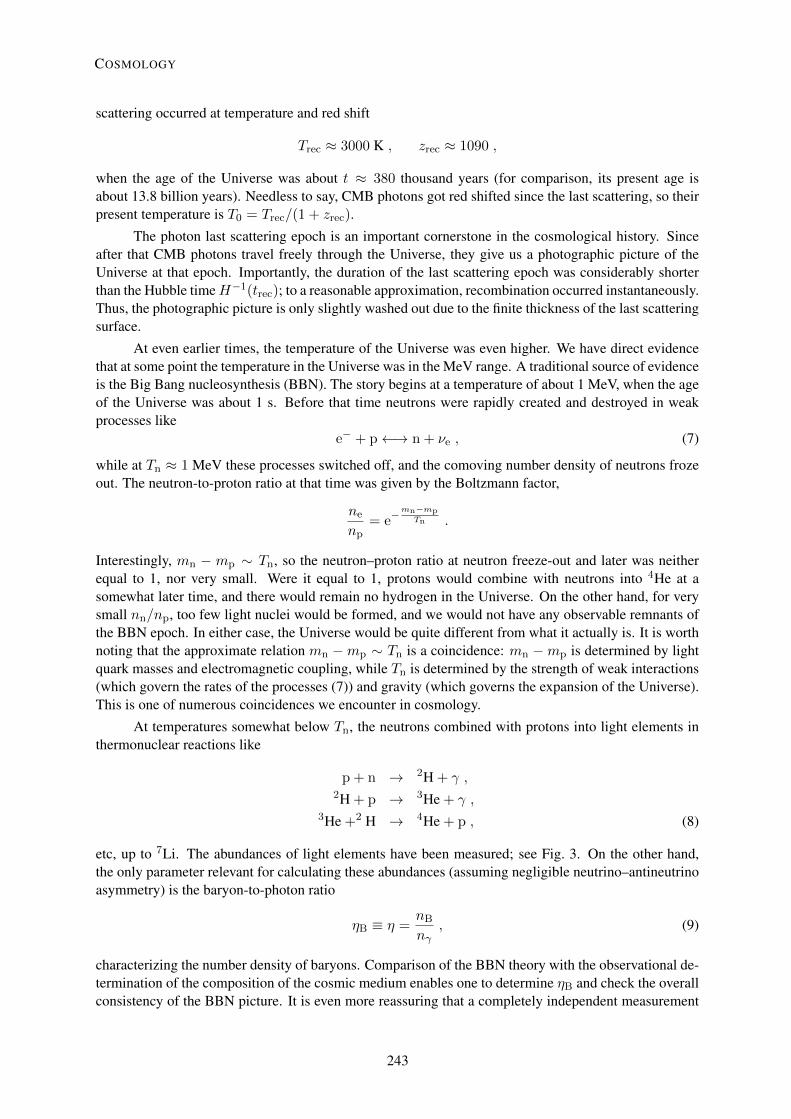
etc, up to 7Li. The abundances of light elements have been measured; see Fig. 3. On the other hand,the only parameter relevant for calculating these abundances (assuming negligible neutrino–antineutrinoasymmetry) is the baryon-to-photon ratio

ηB ≡ η =nB

nγ, (9)

characterizing the number density of baryons. Comparison of the BBN theory with the observational de-termination of the composition of the cosmic medium enables one to determine ηB and check the overallconsistency of the BBN picture. It is even more reassuring that a completely independent measurement

5

COSMOLOGY

243

3He/H p

4He

2 3 4 5 6 7 8 9 101

0.01 0.02 0.030.005

CM

B

BB

NBaryon-to-photon ratio η × 1010

Baryon density Ωbh2

D___H

0.24

0.23

0.25

0.26

0.27

10−4

10−3

10−5

10−9

10−10

2

57Li/H p

Yp

D/H p

Fig. 3: Abundances of light elements, measured (boxes; larger boxes include systematic uncertainties) and cal-culated as functions of baryon-to-photon ratio η [25]. The determination of η ≡ ηB from BBN (vertical rangemarked BBN) is in excellent agreement with the determination from the analysis of CMB temperature fluctuations(vertical range marked CMB).

of ηB that makes use of the CMB temperature fluctuations is in excellent agreement with BBN. Thus,BBN gives us confidence that we understand the Universe at T ∼ 1 MeV, t ∼ 1 s. In particular, we areconvinced that the cosmological expansion was governed by general relativity.

Another class of processes of interest at temperatures in the MeV range is neutrino production,annihilation and scattering,

να + να ←→ e+ + e−

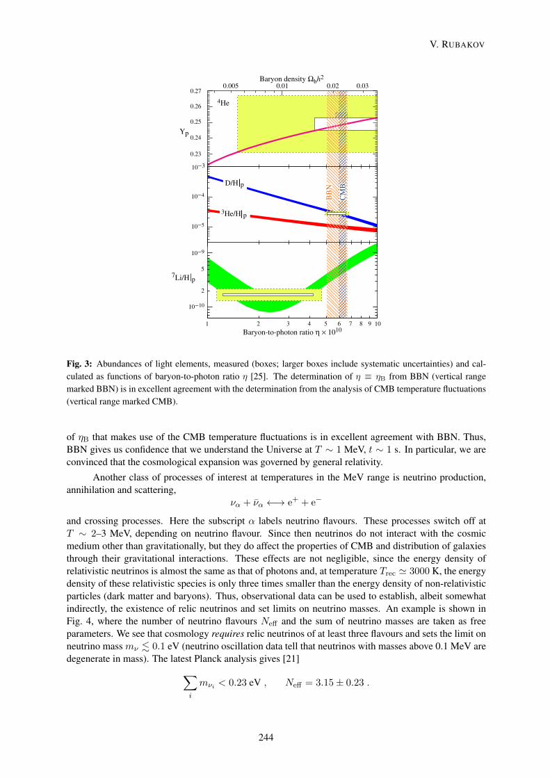
and crossing processes. Here the subscript α labels neutrino flavours. These processes switch off atT ∼ 2–3 MeV, depending on neutrino flavour. Since then neutrinos do not interact with the cosmicmedium other than gravitationally, but they do affect the properties of CMB and distribution of galaxiesthrough their gravitational interactions. These effects are not negligible, since the energy density ofrelativistic neutrinos is almost the same as that of photons and, at temperature Trec ' 3000 K, the energydensity of these relativistic species is only three times smaller than the energy density of non-relativisticparticles (dark matter and baryons). Thus, observational data can be used to establish, albeit somewhatindirectly, the existence of relic neutrinos and set limits on neutrino masses. An example is shown inFig. 4, where the number of neutrino flavours Neff and the sum of neutrino masses are taken as freeparameters. We see that cosmology requires relic neutrinos of at least three flavours and sets the limit onneutrino mass mν . 0.1 eV (neutrino oscillation data tell that neutrinos with masses above 0.1 MeV aredegenerate in mass). The latest Planck analysis gives [21]

∑

i

mνi < 0.23 eV , Neff = 3.15± 0.23 .

6

V. RUBAKOV

244

Fig. 4: Effective number of neutrino species and sum of neutrino masses allowed by cosmological observa-tions [26].

2.3 Dynamics of expansionThe basic equation governing the expansion rate of the Universe is the Friedmann equation,

H2 ≡(a

a

)2

=8π

3M2Pl

ρ− κa2

, (10)

where the dot denotes derivative with respect to time t, ρ is the total energy density in the Universeand κ = 0,±1 is the parameter, introduced in Section 2.1, that discriminates the Euclidean 3-space(κ = 0) and curved 3-spaces. The Friedmann equation is nothing but the (00)-component of the Einsteinequations of general relativity, R00 − 1

2g00R = 8πT00, specified to the FLRW metric. Observationally,the spatial curvature of the Universe is very small: the last, curvature term in the right-hand side ofEq. (10) is small compared to the energy density term [21],

1/a2

8πρ/(3M2Pl)

< 0.005 ,

while the theoretical expectation is that the spatial curvature is completely negligible. Establishing thatthe three-dimensional space is (nearly) Euclidean is one of the profound results of CMB observations.

In what follows we set κ = 0 and write the Friedmann equation as

H2 ≡(a

a

)2

=8π

3M2Pl

ρ . (11)

The standard parameter used in cosmology is the critical density,

ρc =3

8πM2

PlH20 ≈ 5× 10−6 GeV

cm3. (12)

According to Eq. (11), it is equal to the sum of all forms of energy density in the present Universe.There are at least three of such forms: relativistic matter, or radiation, non-relativistic matter, M and

7

COSMOLOGY

245

dark energy, Λ. For every form λ with the present energy density ρλ,0, one defines the parameter

Ωλ =ρλ,0ρc

.

One finds from Eq. (11) that ∑

λ

Ωλ = 1 .

The Ω are important cosmological parameters characterizing the energy balance in the present Universe.Their numerical values are

Ωrad = 8.7× 10−5 , (13a)

ΩM = 0.31 , (13b)

ΩΛ = 0.69 . (13c)

The value of Ωrad needs qualification. At early times, when the temperature exceeds the masses of allneutrino species, neutrinos are relativistic. The value of Ωrad in Eq. (13a) is calculated for the unrealisticcase in which all neutrinos are relativistic today, so the radiation component even at present consists ofCMB photons and three neutrino species. This prescription is convenient for studying the energy (andentropy) content in the early Universe, since it enables one to scale the energy density (and entropy) backin time in a simple way, see below. For future reference, let us give the value of the present entropydensity in the Universe, pretending that neutrinos are relativistic,

s0 ≈ 3000 cm−3 . (14)

Question. Calculate the numerical value of Ωγ and the entropy density of CMB photons.

Non-relativistic matter consists of baryons and dark matter. The contributions of each of thesefractions are [21]

ΩB = 0.048 ,

ΩDM = 0.26 .

Different components of the energy density evolve differently in time. The energy of a given pho-ton or massless neutrino scales as a−1, and the number density of these species scales as a−3. Therefore,the energy density of radiation scales as ρrad ∝ a−4 and

ρrad(t) =

(a(t)

a0

)4

ρrad,0 = (1 + z)4 Ωradρc . (15)

The energy of non-relativistic matter is dominated by the mass of its particles, so the energy densityscales as the number density, i.e.,

ρM(t) =

(a(t)

a0

)3

ρM,0 = (1 + z)3 ΩMρc . (16)

Finally, the energy density of dark energy does not change in time, or changes very slowly. We assumefor definiteness that ρΛ stays constant in time,

ρΛ = ΩΛρc = const . (17)

In fact, whether or not ρΛ depends on time (even slightly) is a very important question. If dark energy isa cosmological constant (or, equivalently, vacuum energy), then it does not depend on time at all. Even

8

V. RUBAKOV

246

a slight dependence of ρΛ on time would mean that we are dealing with something different from thecosmological constant, like, e.g., a new scalar field with a very flat scalar potential. The existing limits onthe time evolution of dark energy correspond, roughly speaking, to the variation of ρΛ by not more than20% in the last 8 billion years (from the time corresponding to z ≈ 1); usually these limits are expressedin terms of the equation-of-state parameter relating energy density and effective pressure pΛ = wΛρΛ:

wΛ ≈ 1.0± 0.1 . (18)

The relevance of the effective pressure is seen from the covariant conservation equation for the energy–momentum tensor,∇µTµν = 0, whose ν = 0 component reads

ρ = −3a

a(ρ+ p) .

It shows that the energy density of a component with equation of state p = wρ, w = const scales asρ ∝ a−3(1+w). As pointed out above, radiation (wrad = 1/3) and matter (w = 0) scale as ρrad ∝ a−4

and ρM ∝ a−3, respectively, while the cosmological constant case corresponds to wΛ = −1.

Question. Show that for a gas of relativistic particles, p = ρ/3.

According to Eqs. (15), (16) and (17), different forms of energy dominate at different cosmologicalepochs. The present Universe is at the end of the transition from matter domination to Λ domination: thedark energy will ‘soon’ completely dominate over non-relativistic matter because of the rapid decreaseof the energy density of the latter. Conversely, the matter energy density increases as we go backwards intime, and until relatively recently (z . 0.3) it dominated over dark energy density. At even more distantpast, the radiation energy density was the highest, as it increases most rapidly backwards in time. Thered shift at radiation–matter equality, when the energy densities of radiation and matter were equal, is

1 + zeq =a0

a(teq)=

ΩM

Ωrad≈ 3500

and, using the Friedmann equation, one finds the age of the Universe at equality

teq ≈ 50 000 years .

Note that recombination occurred at matter domination, but rather soon after equality. So, we have thefollowing sequence of the regimes of evolution:

. . . =⇒ Radiation domination =⇒ Matter domination =⇒ Λ domination .

The dots here denote some cosmological epoch preceding the hot stage of the evolution; as we mentionedin Section 1, we are confident that such an epoch existed, but do not quite know what it was.

2.4 Radiation dominationThe epoch of particular interest for our purposes is radiation domination. By inserting ρrad ∝ a−4 intothe Friedmann equation (11), we obtain

a

a=

consta2

.

This gives the evolution lawa(t) = const ·

√t . (19)

The constant here does not have physical significance, as one can rescale the coordinates x at some fixedmoment of time, thus changing the normalization of a.

9

COSMOLOGY

247

There are several points to note regarding the result (19). First, the expansion decelerates:

a < 0 .

This property holds also for the matter-dominated epoch, but it does not hold for the domination of thedark energy.

Question. Find the evolution laws, analogous to Eq. (19), for matter- and Λ-dominated Universes. Showthat the expansion decelerates, a < 0, at matter domination and accelerates, a > 0, at Λ domination.

Second, time t = 0 is the Big Bang singularity (assuming erroneously that the Universe startsbeing radiation dominated). The expansion rate

H(t) =1

2t

diverges as t → 0, and so do the energy density ρ(t) ∝ H2(t) and temperature T ∝ ρ1/4. Of course,the classical general relativity and usual notions of statistical mechanics (e.g., temperature itself) are notapplicable very near the singularity, but our result suggests that in the picture we discuss (hot epochright after the Big Bang), the Universe starts its classical evolution in a very hot and dense state, andits expansion rate is very high in the beginning. It is customary to consider for illustrational purposesthat the relevant quantities in the beginning of the classical expansion take the Planck values, ρ ∼ M4

Pl,H ∼MPl etc.

Third, at a given moment of time the size of a causally connected region is finite. Consider signalsemitted right after the Big Bang and travelling with the speed of light. These signals travel along thelight cone with ds = 0 and hence a(t)dx = dt. So, the coordinate distance that a signal travels from theBig Bang to time t is

x =

∫ t

0

dt

a(t)≡ η . (20)

In the radiation-dominated Universe,η = const ·

√t .

The physical distance from the emission point to the position of the signal is

lH(t) = a(t)x = a(t)

∫ t

0

dt

a(t)= 2t .

As expected, this physical distance is finite, and it gives the size of a causally connected region at timet. It is called the horizon size (more precisely, the size of the particle horizon). A related property is thatan observer at time t can see only the part of the Universe whose current physical size is lH(t). Both atradiation and matter domination one has, modulo a numerical constant of order 1,

lH(t) ∼ H−1(t) . (21)

To give an idea of numbers, the horizon size at the present epoch is

lH(t0) ≈ 15 Gpc ' 4.5× 1028 cm .

Question. Find the proportionality constant in Eq. (21) for a matter-dominated Universe. Is there aparticle horizon in a Universe without matter but with positive cosmological constant?

10

V. RUBAKOV

248

It is convenient to express the Hubble parameter at radiation domination in terms of tempera-ture. The Stefan–Boltzmann law gives for the energy density of a gas of relativistic particles in thermalequilibrium at zero chemical potentials (chemical potentials in the Universe are indeed small)

ρrad =π2

30g∗T 4 , (22)

with g∗ being the effective number of degrees of freedom,

g∗ =∑

bosons

gi +7

8

∑

fermions

gi ,

where gi is the number of spin states and the factor 7/8 is due to Fermi statistics. Hence, the Friedmannequation (11) gives

H =T 2

M∗Pl

, M∗Pl =MPl

1.66√g∗. (23)

One more point has to do with entropy: the cosmological expansion is slow, so that the entropy isconserved (modulo exotic scenarios with large entropy generation). The entropy density in thermalequilibrium is given by

s =2π2

45g∗T 3 .

The conservation of entropy means that the entropy density scales exactly as a−3,

sa3 = const , (24)

while temperature scales approximately as a−1. The temperature would scale as a−1 if the number ofrelativistic degrees of freedom would be independent of time. This is not the case, however. Indeed, thevalue of g∗ depends on temperature: at T ∼ 10 MeV relativistic species are photons, neutrinos, electronsand positrons, while at T ∼ 1 GeV four flavours of quarks, gluons, muons and τ -leptons are relativistictoo. The number of degrees of freedom in the Standard Model at T & 100 GeV is

g∗(100 GeV) ≈ 100 .

If there are conserved quantum numbers, such as the baryon number after baryogenesis, theirdensity also scales as a−3. Hence, the time-independent characteristic of, say, the baryon abundance isthe baryon-to-entropy ratio

∆B =nB

s.

The commonly used baryon-to-photon ratio ηB, Eq. (9), is related to ∆B by a numerical factor, but thisfactor depends on time through g∗ and stays constant only after e+e− annihilation, i.e., at T . 0.5 MeV.Numerically,

∆B = 0.14ηB,0 = 0.86× 10−10 . (25)

3 Dark energyBefore turning to our main topics, let us briefly discuss dark energy. We know very little about this‘substance’: our knowledge is summarized in Eqs. (13c) and (18). We also know that dark energy doesnot clump, unlike dark matter and baryons. It gives rise to the accelerated expansion of the Universe.Indeed, the solution to the Friedmann equation (11) with constant ρ = ρΛ is

a(t) = eHΛt ,

11

COSMOLOGY

249

H(z

)/(1

+z)

(km

/sec

/Mpc

)

0 1 2z

90

80

70

60

50

Fig. 5: Observational data on the time derivative of the scale factor as function of red shift z [27]. The change ofthe behaviour from decreasing to increasing with decreasing z means the change from decelerated to acceleratedexpansion. The theoretical curve corresponds to a spatially flat Universe with h = 0.7 and ΩΛ = 0.73.

where HΛ = (8πρΛ/3M2Pl)

1/2 = const. This gives a > 0, unlike at radiation or matter domination. Theobservational discovery of the accelerated expansion of the Universe was the discovery of dark energy.Recall that early on (substantial z), the Universe was matter dominated, so its expansion was decelerating.The transition from decelerating to accelerating expansion is confirmed by combined observational data,see Fig. 5, which shows the dependence on red shift of the quantity H(z)/(1 + z) = a(t)/a0.

Question. Find the red shift z at which decelerated expansion turned into an accelerated one.

As a remark, the effective pressure of dark energy or any other component is defined as the (pos-sibly time-dependent) parameter determining the spatial components of the energy–momentum tensor ina locally Lorentz frame (a = 1 in the FLRW context),

Tµν = diag (ρ, p, p, p) .

In the case of the cosmological constant, the dark energy density does not depend on time at all:

Tµν = ρΛηµν ,

where ηµν is the Minkowski tensor. Hence, wΛ = −1. One can view this as the characteristic of vacuum,whose energy–momentum tensor must be Lorentz-covariant. As we pointed out above, any deviationfrom w = −1 would mean that we are dealing with something other than vacuum energy density.

The problem with dark energy is that its present value is extremely small by particle-physicsstandards,

ρDE ≈ 4 GeV m−3 = (2× 10−3 eV)4 .

In fact, there are two hard problems. One is that particle-physics scales are much larger than the scalerelevant to the dark energy density, so the dark energy density is zero to an excellent approximation.Another is that it is non-zero nevertheless, and one has to understand its energy scale. To quantify thefirst problem, we recall the known scales of particle physics and gravity,

Strong interactions : ΛQCD ∼ 1 GeV ,

12

V. RUBAKOV

250

Electroweak : MW ∼ 100 GeV ,Gravitational : MPl ∼ 1019 GeV .

Off hand, physics at scale M should contribute to the vacuum energy density as ρΛ ∼ M4, and there isabsolutely no reason for vacuum to be as light as it is. The discrepancy here is huge, as one sees fromthe above numbers.

To elaborate on this point, let us note that the action of gravity plus, say, the Standard Model hasthe general form

S = SEH + SSM − ρΛ,0

∫ √−g d4x ,

where SEH = −(16πG)−1∫R√−g d4x is the Einstein–Hilbert action of general relativity, SSM is the

action of the Standard Model and ρΛ,0 is the bare cosmological constant. In order that the vacuum energydensity be almost zero, one needs fantastic cancellations between the contributions of the Standard Modelfields into the vacuum energy density, on the one hand, and ρΛ,0 on the other. For example, we know thatquantum chromodynamics (QCD) has a complicated vacuum structure, and one would expect that theenergy density of QCD should be of the order of (1 GeV)4. At least for QCD, one needs a cancellationof the order of 10−44. If one goes further and considers other interactions, the numbers get even worse.

What are the hints from this ‘first’ cosmological constant problem? There are several options,though not many. One is that the Universe could have a very long prehistory: extremely long. Thisoption has to do with relaxation mechanisms. Suppose that the original vacuum energy density is indeedlarge, say, comparable to the particle-physics scales. Then there must be a mechanism which can relaxthis value down to an acceptably small number. It is easy to convince oneself that this relaxation couldnot happen in the history of the Universe we know of. Instead, the Universe should have a very longprehistory during which this relaxation process might occur. At that prehistoric time, the vacuum in theUniverse must have been exactly the same as our vacuum, so the Universe in its prehistory must havebeen exactly like ours, or almost exactly like ours. Only in that case could a relaxation mechanism work.There are concrete scenarios of this sort [28, 29]. However, at the moment it seems that these scenariosare hardly testable, since this is prehistory.

Another possible hint is towards anthropic selection. The argument that goes back to Weinberg andLinde [30, 31] is that if the cosmological constant were larger, say, by a factor of 100, we simply wouldnot exist: the stars would not have formed because of the fast expansion of the Universe. So, the vacuumenergy density may be selected anthropically. The picture is that the Universe may be much, muchlarger than what we can see, and different large regions of the Universe may have different properties. Inparticular, vacuum energy density may be different in different regions. Now, we are somewhere in theplace where one can live. All the rest is empty of observers, because there the parameters such as vacuumenergy density are not suitable for their existence. This is disappointing for a theorist, as this point ofview allows for arbitrary tuning of fundamental parameters. It is hard to disprove this option, on the otherhand. We do exist, and this is an experimental fact. The anthropic viewpoint may, though hopefully willnot, get more support from the LHC, if no or insufficient new physics is found there. Indeed, anothercandidate for an environmental quantity is the electroweak scale, which is fine tuned in the StandardModel in the same sense as the cosmological constant is fine tuned in gravity (in the Standard Modelcontext, this fine tuning goes under the name of the gauge hierarchy problem).

Turning to the ‘second’ cosmological constant problem, we note that the scale 10−3 eV maybe associated with some new light field(s), rather than with vacuum. This implies that ρΛ dependson time, i.e., wΛ 6= −1 and wΛ may well depend on time itself. Current data are compatible withtime-independent wΛ equal to −1, but their precision is not particularly high. We conclude that futurecosmological observations may shed new light on the field content of the fundamental theory.

13

COSMOLOGY

251

4 Dark matterUnlike dark energy, dark matter experiences the same gravitational force as baryonic matter. It consistspresumably of new stable massive particles. These make clumps of mass which constitute most of themass of galaxies and clusters of galaxies. There are various ways of measuring the contribution of non-baryonic dark matter into the total energy density of the Universe (see Refs. [7–10] for details).

1. The composition of the Universe affects the angular anisotropy and polarization of CMB. Quiteaccurate CMB measurements available today enable one to measure the total mass density of darkmatter.

2. There is direct evidence that dark matter exists in the largest gravitationally bound objects—clusters of galaxies. There are various methods to determine the gravitating mass of a cluster,and even the mass distribution in a cluster, which give consistent results. As an example, the totalgravitational field of a cluster, produced by both dark matter and baryons, acts as a gravitationallens for extended light sources behind the cluster. The images of these sources enable one to re-construct the mass distribution in the cluster. This is shown in Fig. 6. These determinations showthat baryons (independently measured through their X-ray emission) make less than 1/3 of totalmass in clusters. The rest is dark matter.

Fig. 6: Cluster of galaxies CL0024 + 1654 [32], acting as gravitational lens. Right-hand panel: cluster in visiblelight. Round yellow spots are galaxies in the cluster. Elongated blue images are those of one and the same galaxybeyond the cluster. Left-hand panel: reconstructed distribution of gravitating mass in the cluster; brighter regionshave larger mass density.

A particularly convincing case is the Bullet Cluster, Fig. 7. Shown are two galaxy clusters thatpassed through each other. The dark matter and galaxies do not experience friction and thus do notlose their velocities. On the contrary, baryons in hot, X-ray-emitting gas do experience friction andhence get slowed down and lag behind dark matter and galaxies. In this way the baryons (whichare mainly in hot gas) and dark matter are separated in space.

3. Dark matter exists also in galaxies. Its distribution is measured by the observations of rotationvelocities of distant stars and gas clouds around a galaxy, Fig. 8. Because of the existence of darkmatter away from the luminous regions, i.e., in halos, the rotation velocities do not decrease withthe distance from the galactic centres; rotation curves are typically flat up to distances exceedingthe size of the bright part by a factor of 10 or so. The fact that dark matter halos are so largeis explained by the defining property of dark matter particles: they do not lose their energies byemitting photons and, in general, interact with conventional matter very weakly.

14

V. RUBAKOV

252

Fig. 7: Observation [33] of the Bullet Cluster 1E0657-558 at z = 0.296. Closed lines show the gravitationalpotential produced mainly by dark matter and measured through gravitational lensing. Bright regions show X-rayemission of hot baryon gas, which makes most of the baryonic matter in the clusters. The length of the whiteinterval is 200 kpc in the comoving frame.

Dark matter is characterized by the mass-to-entropy ratio,

(ρDM

s

)0

=ΩDMρc

s0≈ 0.26× 5× 10−6 GeV cm−3

3000 cm−3= 4× 10−10 GeV . (26)

This ratio is constant in time since the freeze out of dark matter density: both number density of darkmatter particles nDM (and hence their mass density ρDM = mDMnDM) and entropy density get dilutedexactly as a−3.

Dark matter is crucial for our existence, for the following reason. Density perturbations in baryon–electron–photon plasma before recombination do not grow because of high pressure, which is mostlydue to photons; instead, perturbations are sound waves propagating in plasma with time-independentamplitudes. Hence, in a Universe without dark matter, density perturbations in the baryonic componentwould start to grow only after baryons decouple from photons, i.e., after recombination. The mechanism

Fig. 8: Rotation velocities of hydrogen gas clouds around the galaxy NGC 6503 [34]. Lines show the contributionsof the three main components that produce the gravitational potential. The main contribution at large distances isdue to dark matter, labelled ‘halo’.

15

COSMOLOGY

253

of the growth is pretty simple: an overdense region gravitationally attracts surrounding matter; this matterfalls into the overdense region, and the density contrast increases. In the expanding matter-dominatedUniverse this gravitational instability results in the density contrast growing like (δρ/ρ)(t) ∝ a(t).Hence, in a Universe without dark matter, the growth factor for baryon density perturbations would be atmost

a(t0)

a(trec)= 1 + zrec =

Trec

T0≈ 103 . (27)

Because of the presence of dark energy, the growth factor is even somewhat smaller. The initial amplitudeof density perturbations is very well known from the CMB anisotropy measurements, (δρ/ρ)i = 5 ×10−5. Hence, a Universe without dark matter would still be pretty homogeneous: the density contrastwould be in the range of a few per cent. No structure would have been formed, no galaxies, no life. Nostructure would be formed in future either, as the accelerated expansion due to dark energy will soonterminate the growth of perturbations.

Since dark matter particles decoupled from plasma much earlier than baryons, perturbations indark matter started to grow much earlier. The corresponding growth factor is larger than (27), so that thedark matter density contrast at galactic and subgalactic scales becomes of order one, perturbations enterthe non-linear regime and form dense dark matter clumps at z = 5–10. Baryons fall into potential wellsformed by dark matter, so dark matter and baryon perturbations develop together soon after recombina-tion. Galaxies get formed in the regions where dark matter was overdense originally. For this picture tohold, dark matter particles must be non-relativistic early enough, as relativistic particles fly through grav-itational wells instead of being trapped there. This means, in particular, that neutrinos cannot constitutea considerable part of dark matter.

4.1 Cold and warm dark matterCurrently, the most popular dark matter scenario is cold dark matter, CDM. It consists of particles whichget out of kinetic equilibrium when they are non-relativistic. For dark matter particles Y which areinitially in thermal equilibrium with cosmic plasma, this means that their scattering off other particlesswitches off at T = Td mY. Since then the dark matter particles move freely, their momenta decreasedue to red shift, and they remain non-relativistic until now. Note that the decoupling temperature Td maybe much lower than the freeze-out temperature Tf at which the dark matter particles get out of chemicalequilibrium, i.e., their number in the comoving volume freezes out (because, e.g., their creation andannihilation processes switch off). This is the case for many models with weakly interacting massiveparticles (WIMPs), a class of dark matter particles we discuss in some detail below. Note also that darkmatter particles may never be in thermal equilibrium; this is the case, e.g., for axions.

An alternative to CDM is warm dark matter, WDM, whose particles decouple, being relativistic.Let us assume for definiteness that they are in kinetic equilibrium with cosmic plasma at temperatureTf when their number density freezes out (thermal relic). After kinetic equilibrium breaks down attemperature Td ≤ Tf , their spatial momenta decrease as a−1, i.e., the momenta are of order T all the timeafter decoupling. Warm dark matter particles become non-relativistic at T ∼ m, where m is their mass.Only after that do the WDM perturbations start to grow: as we mentioned above, relativistic particlesescape from gravitational potentials, so the gravitational wells get smeared out instead of getting deeper.Before becoming non-relativistic, WDM particles travel the distance of the order of the horizon size;the WDM perturbations therefore are suppressed at those scales. The horizon size at the time tnr whenT ∼ m is of order

lH(tnr) ' H−1(T ∼ m) =M∗Pl

T 2∼ M∗Pl

m2.

Due to the expansion of the Universe, the corresponding length at present is

l0 = lH(tnr)a0

a(tnr)∼ lH(tnr)

T

T0∼ MPl

mT0, (28)

16

V. RUBAKOV

254

where we neglected (rather weak) dependence on g∗. Hence, in the WDM scenario, structures of sizessmaller than l0 are less abundant as compared to CDM. Let us point out that l0 refers to the size of theperturbation in the linear regime; in other words, this is the size of the region from which matter collapsesinto a compact object.

There is a hint towards the plausibility of warm, rather than cold, dark matter. It is the dwarf-galaxy problem. According to numerical simulations, the CDM scenario tends to overproduce smallobjects—dwarf galaxies: it predicts hundreds of satellite dwarf galaxies in the vicinity of a large galaxylike the Milky Way, whereas only dozens of satellites have been observed so far. This argument is stillcontroversial, but, if correct, it does suggest that the dark matter perturbations are suppressed at dwarf-galaxy scales. This is naturally the case in the WDM scenario. The present size of a dwarf galaxy is afew kpc, and the density is about 106 of the average density in the Universe. Hence, the size l0 for theseobjects is of order 100 kpc ' 3× 1023 cm. Requiring that perturbations of this size, but not much larger,are suppressed, we obtain from (28) the estimate for the mass of a dark matter particle

WDM : mDM = 3–10 keV . (29)

On the other hand, this effect is absent, i.e., dark matter is cold, for

CDM : mDM 10 keV . (30)

Let us recall that these estimates apply to particles that are initially in kinetic equilibrium with cosmicplasma. They do not apply in the opposite case; an example is axion dark matter, which is cold despitebeing of very small axion mass.

4.2 WIMP miracleThere is a simple mechanism of the dark matter generation in the early Universe. It applies to cold darkmatter. Because of its simplicity and robustness, it is considered by many as a very likely one, and thecorresponding dark matter candidates—WIMPs—as the best candidates. Let us describe this mechanismin some detail.

Let us assume that there exists a heavy stable neutral particle Y, and that Y particles can only bedestroyed or created via their pair annihilation or creation, with annihilation products being the particlesof the Standard Model. The general scenario for the cosmological behaviour of Y particles is as follows.At high temperatures, T mY, the Y particles are in thermal equilibrium with the rest of the cosmicplasma; there are lots of Y particles in the plasma, which are continuously created and annihilate. As thetemperature drops below mY, the equilibrium number density decreases. At some ‘freeze-out’ tempera-ture Tf , the number density becomes so small that Y particles can no longer meet each other during theHubble time, and their annihilation terminates. After that the number density of surviving Y particlesdecreases like a−3, and these relic particles contribute to the mass density in the present Universe.

Let us estimate the properties of Y particles such that they really serve as dark matter. Elementaryconsiderations of mean free path of a particle in gas give for the lifetime of a non-relativistic Y particlein cosmic plasma, τann,

〈σann · v〉 · τann · nY ∼ 1 ,

where v is the relative velocity of Y particles, σann is the annihilation cross-section at velocity v, averag-ing is over the velocity distribution of Y particles and nY is the number density. In thermal equilibriumat T mY, the latter is given by the Boltzmann law at zero chemical potential,

n(eq)Y = gY ·

(mYT

2π

)3/2

e−mYT , (31)

where gY is the number of spin states of a Y particle. Let us introduce the notation

〈σann · v〉 = σ0

17

COSMOLOGY

255

(in kinetic equilibrium, the left-hand side is the thermal average). If the annihilation occurs in an s-wave,then σ0 is a constant independent of temperature; for a p-wave it is somewhat suppressed at T mY,namely σ0 ∝ v2 ∝ T/mY. A quick way to come to correct estimate is to compare the lifetime with theHubble time, or the annihilation rate Γann ≡ τ−1

ann with the expansion rate H . At T ∼ mY, the equilib-rium density is of order nY ∼ T 3, and Γann H for not too small σ0. This means that annihilation(and, by reciprocity, creation) of Y pairs is indeed rapid, and Y particles are indeed in complete thermalequilibrium with the plasma. At very low temperature, on the other hand, the equilibrium number den-sity n(eq)

Y is exponentially small, and the equilibrium rate is small too, Γ(eq)ann H . At low temperatures

we cannot, of course, make use of the equilibrium formulas: Y particles no longer annihilate (and, byreciprocity, are no longer created), there is no thermal equilibrium with respect to creation–annihilationprocesses and the number density nY gets diluted only because of the cosmological expansion.

The freeze-out temperature Tf is determined by the relation1

τ−1ann ≡ Γann ' H , (32)

where we use the equilibrium formulas. Making use of the relation (23) between the Hubble parameterand the temperature at radiation domination, we obtain

σ0(Tf) · nY(Tf) ∼T 2

f

M∗Pl

(33)

or

σ0(Tf) · gY ·(mYTf

2π

)3/2

e−mYTf ∼ T 2

f

M∗Pl

. (34)

The latter equation gives the freeze-out temperature, which, up to log–log corrections, is

Tf ≈mY

ln(M∗PlmYσ0)(35)

(the possible dependence of σ0 on temperature is irrelevant in the right-hand side: we are doing thecalculation in the leading-log approximation anyway). Note that this temperature is somewhat lowerthan mY if the relevant microscopic mass scale is much below MPl. This means that Y particles freezeout when they are indeed non-relativistic and get out of kinetic equilibrium at even lower temperature,hence the term ‘cold dark matter’. The fact that the annihilation and creation of Y particles terminate ata relatively low temperature has to do with the rather slow expansion of the Universe, which should becompensated for by the smallness of the number density nY.

At the freeze-out temperature, we make use of Eq. (33) and obtain

nY(Tf) =T 2

f

M∗Plσ0(Tf). (36)

Note that this density is inversely proportional to the annihilation cross-section (modulo a logarithm).The reason is that for higher annihilation cross-sections, the creation–annihilation processes are longerin equilibrium, and fewer Y particles survive.

1In fact, we somewhat oversimplify the analysis here. The chemical equilibrium breaks down slightly earlier than what wefind from Eq. (32): the corresponding temperature is obtained by equating the equilibrium creation–annihilation rate Γann tothe rate of evolution of the equilibrium number density (31), rather than to the Hubble parameter H . For T mY , this givesthe equation for the temperature

Γann ' nY

nY' −mY

T

T

T=mY

TH(T ) .

This temperature differs by the log–log correction from Tf determined from Eq. (34) and, at this temperature, one has nY T 2/(M∗Plσ0), cf. Eq. (36). However, below this temperature, the annihilation of Y particles continues, and it terminates attemperature Tf determined by Eq. (32), which gives Eqs. (33) and (36). All this gives rise to log–log corrections, which we donot calculate anyway. So, our estimate for the present dark matter mass density remains valid.

18

V. RUBAKOV

256

Up to a numerical factor of order 1, the number-to-entropy ratio at freeze-out is

nY

s' 1

g∗(Tf)M∗PlTfσ0(Tf)

. (37)

This ratio stays constant until the present time, so the present number density of Y particles is nY,0 =s0 · (nY/s)freeze-out, and the mass-to-entropy ratio is

ρY,0

s0=mYnY,0

s0' ln(M∗PlmYσ0)

g∗(Tf)M∗Plσ0(Tf)

' ln(M∗PlmYσ0)√g∗(Tf)MPlσ0(Tf)

,

where we made use of (35). This formula is remarkable. The mass density depends mostly on oneparameter, the annihilation cross-section σ0. The dependence on the mass of a Y particle is through thelogarithm and through g∗(Tf); it is very mild. The value of the logarithm here is between 30 and 40,depending on parameters (this means, in particular, that freeze-out occurs when the temperature drops30 to 40 times below the mass of a Y particle). Inserting g∗(Tf) ∼ 100, as well as the numerical factoromitted in Eq. (37), and comparing with (26), we obtain the estimate

σ0(Tf) ≡ 〈σv〉(Tf) = (1–2)× 10−36 cm2 . (38)

This is a weak-scale cross-section, which tells us that the relevant energy scale is TeV. We note in passingthat the estimate (38) is quite precise and robust.

If the annihilation occurs in an s-wave, the annihilation cross-section may be parametrized asσ0 = α2/M2, where α is some coupling constant and M is a mass scale (which may be higher thanmY). This parametrization is suggested by the picture of Y-pair annihilation via the exchange by anotherparticle of mass M . With α ∼ 10−2, the estimate for the mass scale is roughly M ∼ 1 TeV. Thus, withvery mild assumptions, we find that the non-baryonic dark matter may naturally originate from the TeV-scale physics. In fact, what we have found can be understood as an approximate equality between thecosmological parameter, the mass-to-entropy ratio of dark matter and the particle-physics parameters,

mass-to-entropy ' 1

MPl

(TeVαW

)2

.

Both are of order 10−10 GeV, and it is very tempting to think that this ‘WIMP miracle’ is not a merecoincidence. If it is not, the dark matter particles should be found at the LHC.

The most prominent candidate for WIMPs is neutralinos of the supersymmetric extensions ofthe Standard Model. The situation with neutralinos is somewhat tense, however. The point is thatthe pair annihilation of neutralinos often occurs in the p-wave, rather than the s-wave. This gives thesuppression factor in σ0 ≡ 〈σannv〉 proportional to v2 ∼ Tf/mY ∼ 1/30. Hence, neutralinos tend to beoverproduced in most of the parameter space of the Minimal Supersymmetric Standard Model (MSSM)and other models. Yet neutralinos remain a good candidate, especially at high tanβ.

A direct search for dark matter WIMPs is underway in underground laboratories. The idea is thatWIMPs orbiting around the centre of our Galaxy with velocity of order 10−3 sometimes hit a nucleusin a detector and deposit a small energy in it. These searches have become sensitive to neutralinos, asshown in Fig. 9. Indirect searches for dark matter WIMPs include the search for neutrinos coming fromthe centres of the Earth and Sun (WIMPs may concentrate and annihilate there), see, e.g., Ref. [36] andpositrons and antiprotons in cosmic rays (produced in WIMP annihilations in our Galaxy), see, e.g.,Ref. [37]. Collider searches are sensitive to WIMPs too, see Fig. 10. We conclude that the hunt forWIMPs has entered the promising stage.

Question. Estimate the energy deposited in the XENON detector due to elastic scattering of a dark matterWIMP, for WIMP masses 10 GeV, 100 GeV and 1 TeV. Estimate the number of events per kilogram per

19

COSMOLOGY

257

Fig. 9: MSSM predictions for spin-independent elastic neutralino–nucleon cross-section versus neutralino massand experimentally excluded regions [35]. Shaded regions correspond to MSSM parameters consistent with col-lider limits and yielding ΩDM ≈ 0.25. Regions above the open solid lines are ruled out by direct searches, closedsolid curves correspond to regions favoured by experiments indicated. Dashed lines are sensitivities of future directsearch experiments LUX and XENON 1T.

Fig. 9: MSSM predictions for spin-independent elastic neutralino-nucleon cross section versus neutralino mass andexperimentally excluded regions [20]. Shaded regions correspond to MSSM parameters consistent with colliderlimits and yieldingΩDM ≈ 0.25. Regions above the open solid lines are ruled out by direct searches, closedsolid curves correspond to regions favored by experiments indicated. Dashed lines are sensitivities of future directsearch experiments LUX and XENON 1T.

[GeV]χM1 10 210 310

]2-N

ucle

on C

ross

Sec

tion

[cm

χ

-4610

-4510

-4410

-4310

-4210

-4110

-4010

-3910

-3810

-3710

-3610

-1CMS, 90% CL, 8 TeV, 19.7 fb

-1CMS, 90% CL, 7 TeV, 5.0 fb

COUPP 2012

-W+

IceCube W

SIMPLE 2012

-W+

Super-K W

CMS

Spin Dependent

2Λ

q)5

γµγq)(χ5

γµ

γχ(Axial-vector operator

[GeV]χM1 10 210 310

]2-N

ucle

on C

ross

Sec

tion

[cm

χ

-4610

-4510

-4410

-4310

-4210

-4110

-4010

-3910

-3810

-3710

-3610

-1CMS, 90% CL, 8 TeV, 19.7 fb

-1CMS, 90% CL, 7 TeV, 5.0 fb

LUX 2013

superCD

MS

CD

MS

lite

XENON100

COUPP 2012

SIMPLE 2012CoGeNT 2011

CDMS II

CMS

Spin Independent

2Λ

q)µγq)(χµ

γχ(

Vector

3Λ4

2)νµa(G

sαχχ

Scalar

-1CMS, 90% CL, 8 TeV, 19.7 fb

Fig. 10: Excluded regions in the parameter space(MX , σpX) [23] for spin-dependent (left) and spin-independent(right) WIMP interactions with nucleon. Regions above the curves are ruled out at at 90 % confidence level. CMSdenotes searches for WIMPs at the Large Hadron Collider (assuming contact interactionY Y f1f2, wheref1,2 areStandard Model fermions); IceCube and Super-K are searchesfor neutrinos from WIMP annihilation in the Sun;others are direct searches. The shaded region in the middle of the right panel is favored by possible signal at CDMSexperiment.

assuming that the WIMP mass density around the Earth is similar to the av-erage baryon mass density,ρDM ∼ 0.3 GeV/cm3, and thatvDM ∼ 10−3.

24

Fig. 10: Excluded regions in the parameter space (MX, σpX) [38] for spin-dependent (left) and spin-independent(right) WIMP interactions with nucleons. Regions above the curves are ruled out at 90 % confidence level. CMSdenotes searches for WIMPs at the LHC (assuming contact interaction YYf1f2, where f1,2 are Standard Modelfermions); IceCube and Super-K are searches for neutrinos from WIMP annihilation in the Sun; others are directsearches. The shaded region in the middle of the right-hand panel is favoured by a possible signal at the CDMSexperiment.

year for the same masses and elastic cross-sections 10−5 pb, 10−9 pb and 10−8 pb, respectively (seeFig. 9), assuming that the WIMP mass density around the Earth is similar to the average baryon massdensity, ρDM ∼ 0.3 GeV cm−3, and that vDM ∼ 10−3.

20

V. RUBAKOV

258

4.3 Light long-lived particlesMany extensions of the Standard Model contain light scalar or pseudoscalar particles. In some modelsthese new particles are so weakly interacting that their lifetime exceeds the present age of the Universe.Hence, they may serve as dark matter candidates. The best motivated of them is the axion, but there isan entire zoo of axion-like particles.

Let us consider general properties of models with light scalars or pseudoscalars. These particlesshould interact with the usual matter very weakly, so they must be neutral with respect to the StandardModel gauge interactions. This implies that interactions of scalars S and pseudoscalars P with gaugefields are of the form

LSFF =CSFF

4Λ· SFµνFµν , LPFF =

CPFF8Λ

· PFµνFλρεµνλρ , (39)

where Fµν is the field strength of the SU(3)c, SU(2)W or U(1)Y gauge group. The parameter Λ hasdimension of mass and can be interpreted as the scale of new physics related to an S and/or a P particle.This parameter has to be large; then the interactions of S and P with gauge bosons are indeed weakat low energies. Because of that, the Lagrangians (39) contain gauge-invariant operators of the lowestpossible dimension. Dimensionless constants CSFF and CPFF are typically numbers of order 1. Theterms (39) describe interactions of (pseudo)scalars with pairs of photons, gluons as well as with Zγ, ZZand W+W− pairs.

Interactions with fermions can also be written on symmetry grounds. Since S and P are singletsunder SU(3)c × SU(2)W × U(1)Y, no combinations like Sff or P fγ5f are gauge invariant, so theycannot appear in the Lagrangian (hereafter f denotes the Standard Model fermions). Gauge-invariantoperators of the lowest dimension have the formHff , whereH is the Englert–Brout–Higgs field. Hence,the interactions with fermions are

LSHff =YSHff

Λ· SHff , LPHff =

YPHffΛ

· PHfγ5f .

It often happens that the couplings YSHff and YSPff are of the order of the Standard Model Yukawacouplings, so upon electroweak symmetry breaking the low-energy Lagrangians have the following struc-ture:

LSff =CSffmf

Λ· Sff , LPff =

CPffmf

Λ· P fγ5f , (40)

where we assume that the dimensionless couplings CSff and CPff are also of order 1.

Making use of Eqs. (39) and (40), we estimate the partial widths of decays of P and S into theStandard Model particles:

ΓP (S)→AA ∼m3P (S)

64πΛ2, ΓP (S)→ff ∼

m2fmP (S)

8πΛ2, (41)

where A denotes vector bosons. By requiring that the lifetime of the new particles exceeds the presentage of the Universe, τS(P ) = Γ−1

S(P ) > H−10 , we find a bound on the mass of the dark matter candidates,

mP (S) <(16πΛ2H0

)1/3. (42)

Assuming that the new physics scale is below the Planck scale, Λ < MPl, we obtain an (almost) model-independent bound,

mP (S) < 100 MeV . (43)

Hence, the kinematically allowed decays are P (S) → γγ, P (S) → νν and P (S)→ e+e−. It followsfrom Eq. (41) that the two-photon decay mode dominates, unless the mass of the new particle is close tothat of the electron.

21

COSMOLOGY

259

Let us now consider generation of relic (pseudo)scalars in the early Universe. There are severalgeneration mechanisms; one of them is fairly generic for the class of models we discuss. This is genera-tion in decays of condensates (we will consider another mechanism later, in the model with axions). Thepicture is as follows. Let some scalar field φ be in a condensate in the early Universe. The condensatecan be viewed as a collection of φ particles at rest. Equivalently, the condensate is the homogeneousscalar field that oscillates at relatively late times, when mφ > H . Let both particles, φ and S, interactwith matter so weakly that they never get into thermal equilibrium, and let the interaction between φ andS have the form µφS2/2, where µ is the coupling constant. Then the width of the decay φ → SS isestimated as

Γφ→SS ∼µ2

16πmφ. (44)

If the widths of other decay channels do not exceed the value (44), the decay of the φ condensate occursat a temperature Tφ determined by

Γφ→SS ∼ H(Tφ) =T 2φ

M∗Pl

.

Let the energy density of the φ condensate at that time be equal to ρφ, so that the number density ofdecaying φ particles is nφ ∼ ρφ/mφ. Immediately after the epoch of φ-particle decays, the numberdensity of S particles is of order ερφ/mφ, where ε is the fraction of the condensate that decayed into Sparticles. After S particles become non-relativistic, their mass density is of order

ρS ∼ ερφ ·mST

3

mφT3φ

,

where we omitted the dependence on g∗ for simplicity. In this way we estimate the mass fraction of Sparticles today,

ΩS =ρSρc∼ mST

30

ρc· ερφmφT

3φ

∼ 0.2 ·( mS

1 eV

)· ερφmφT

3φ

. (45)

With an appropriate choice of parameters, the correct value ΩS ' 0.2 can indeed be obtained. We notethat the last factor on the right-hand side of Eq. (45) must be small.

4.4 AxionsLet us now turn to a concrete class of models with Peccei–Quinn symmetry and axions. This symmetryprovides a solution to the strong CP-problem, and the existence of axions is an inevitable consequenceof the construction.

The strong CP-problem [39–41] emerges in the following way. One can extend the StandardModel Lagrangian by adding the following term:

∆L =αs

8π· θ0 ·Ga

µνGµν a , (46)

where αs is the SU(3)c gauge coupling, Gaµν is the gluon field strength, Gµν a = 1

2εµνλρGa

λρ is thedual tensor and θ0 is an arbitrary dimensionless parameter (the factor αs/(8π) is introduced for laterconvenience). The interaction term (46) is invariant under gauge symmetries of the Standard Model, butit violates P and CP. The term (46) is a total derivative, so it does not contribute to the classical fieldequations, and its contribution to the action is reduced to the surface integral. For any perturbative gaugefield configurations (small perturbations about Ga

µ = 0), this contribution is equal to zero. However,this is not the case for configurations of instanton type. This means that CP is violated in QCD at thenon-perturbative level.

22

V. RUBAKOV

260

Furthermore, quantum effects due to quarks give rise to the anomalous term in the Lagrangian,which has the same form as Eq. (46) with proportionality coefficient determined by the phase of thequark mass matrix Mq. The latter enters the Lagrangian as

Lm = qLMqqR + h.c.

By chiral rotation of quark fields, one makes quark masses real (i.e., physical), but that rotation inducesa new term in the Lagrangian,

∆Lm =αs

8π·Arg

(DetMq

)·Ga

µνGµν a . (47)

There is no reason to think that Arg(

DetMq

)= 0. Neither there is a reason to think that the ‘tree-level’

term (46) and the anomalous contribution (47) cancel each other. Indeed, the former term is there evenin the absence of quarks, while the latter comes from the Yukawa sector, as the quark masses are due totheir Yukawa interactions with the Englert–Brout–Higgs field.

Thus, the Standard Model Lagrangian should contain the term

∆Lθ =αs

8π

(θ0 + Arg

(DetMq

))GaµνG

µν a ≡ αs

8π· θ ·Ga

µνGµν a . (48)

This term violates CP, and off hand the parameter θ is of order 1.

The term (48) has non-trivial phenomenological consequences. One is that it generates the electricdipole moment (EDM) of the neutron, dn, which is estimated as [42]

dn ∼ θ × 10−16 e cm . (49)

The neutron EDM has not been found experimentally, and the searches place a strong bound

dn . 3× 10−26 e cm . (50)

This leads to the bound on the parameter θ,

|θ| < 0.3× 10−9 .

The problem to explain such a small value of θ is precisely the strong CP-problem.

A solution to this problem does not exist within the Standard Model. The solution is offered bymodels with axions. These models make use of the following observation. If at the classical level thequark Lagrangian is invariant under axial symmetry U(1)A such that

qL → eiβqL , qR → e−iβqR , (51)

then the θ term would be rotated away by applying this transformation. This global symmetry is calledthe Peccei–Quinn (PQ) symmetry [43], U(1)PQ. There is no PQ symmetry in the Standard Model, butone can extend the Standard Model in such a way that the classical Lagrangian is invariant under the PQsymmetry. Quark masses are not invariant under the PQ transformations (51), so PQ symmetry is spon-taneously broken. At the classical level, this leads to the existence of a massless Nambu–Goldstone fielda(x), an axion. As for any Nambu–Goldstone field, its properties are determined by its transformationlaw under the PQ symmetry:

a(x)→ a(x) + β · fPQ , (52)

where β is the same parameter as in Eq. (51) and fPQ is a constant of dimension of mass, the energyscale of U(1)PQ symmetry breaking. The mass terms in the low-energy quark Lagrangian must be

23

COSMOLOGY

261

symmetric under the transformations (51) and (52), so the quark and axion fields enter the Lagrangian inthe combination

Lm = qRmqe−2i a

fPQ qL + h.c. (53)

Making use of Eq. (47), we find that at the quantum level the low-energy Lagrangian contains the term

La = Cgαs

8π· a

fPQGaµνG

µν a , (54)

where the constantCg is of order 1; it is determined by PQ charges of quarks. Clearly, PQ symmetry (51)and (52) is explicitly broken by quantum effects of QCD, and an axion is a pseudo-Nambu–Goldstoneboson.

Hence, the θ parameter multiplying the operatorGaµνG

µν a obtains a shift depending on the space–time point and proportional to the axion field,

θ → θ(x) = θ + Cga(x)

fPQ. (55)

Strong interactions would conserve CP provided the axion vacuum expectation value is such that 〈θ〉 = 0.The QCD effects indeed do the job. They generate a non-vanishing quark condensate 〈qq〉 ∼ Λ3

QCD atthe QCD energy scale ΛQCD ∼ 200 MeV. This condensate breaks chiral symmetry and in turn generatesthe axion effective potential

Va ∼ −1

2θ2 mumd

mu +md〈qq〉+O(θ4) ' 1

8θ2 ·m2

πf2π +O(θ4) , (56)

where mπ = 135 MeV and fπ = 93 MeV are pion mass and decay constant. In fact, the axion potentialmust be periodic in θ with period 2π, so the expression (56) is valid for small θ only. The potential hasthe minimum at 〈θ〉 = 0, so the strong CP-problem finds an elegant solution. It follows from Eqs. (55)and (56) that the axion has a mass

ma ≈ Cgmπfπ2fPQ

, (57)

i.e., it is indeed a pseudo-Nambu–Goldstone boson.

There are various ways to implement the PQ mechanism. One is to introduce two Englert–Brout–Higgs doublets and choose the Yukawa interaction as

Y dQLH1DR + Y uQLiτ2H∗2UR . (58)

The two scalar fields transform under the U(1)PQ transformation (51) as follows:

H1 → e2iβH1 , H2 → e−2iβH2 .

This ensures U(1)PQ invariance of the Lagrangian (58) and hence the absence of the θ term. Bothscalars acquire vacuum expectation values v1 and v2. If no other new fields are added, we arrive at theWeinberg–Wilczek model [44,45]. In that case, the axion field θ is the relative phase of H1 and H2, andthe PQ scale equals the electroweak scale:

fPQ = 2√v2

1 + v22 = 2vSM = 2× 246 GeV .

The axion is quite heavy,ma ∼ 15 keV, and its interaction with quarks, gluons and photons is too strong.Because of that, the Weinberg–Wilczek axion is experimentally ruled out.

This problem is solved in the Dine–Fischler–Srednicki–Zhitnitsky (DFSZ) model [46, 47] byadding a complex scalar field S which is a singlet under the Standard Model gauge group. Its inter-actions involve PQ invariants

S†S , H†1H2 · S2 .

24

V. RUBAKOV

262

The field S transforms under U(1)PQ as S → e2iβS. The axion field is now a linear combination of thephases of fields H1, H2 and S and

fPQ = 2√v2

1 + v22 + v2

s , (59)

where vs is the vacuum expectation value of the field S. The latter can be large, so it is clear fromEq. (59) that the mass of the axion is small and, most importantly, its couplings to the Standard Modelfields are weak: these couplings are inversely proportional to fPQ ∼ vs. The DFSZ axion interacts withboth quarks and leptons.

Another approach is called the Kim–Shifman–Vainshtein–Zakharov (KSVZ) mechanism [48,49].It does not require more than one Englert–Brout–Higgs field of the Standard Model. The mechanismmakes use of additional quark fields ΨR and ΨL, which are triplets under SU(3)c and singlets underSU(2)W ×U(1)Y. Only these quarks transform non-trivially under U(1)PQ, while the usual quarks havezero PQ charge. One also introduces a complex scalar field S, which is a singlet under the StandardModel gauge group. One writes the PQ-invariant Yukawa interaction of the new fields,

L = yΨSΨRΨL + h.c. ,

so that S again transforms under U(1)PQ as S → e2iβS. PQ symmetry is spontaneously broken by thevacuum expectation value 〈S〉 = vs/

√2. The axion here is the phase of the field S; therefore,

fPQ = 2vs . (60)

The KSVZ model does not contain an explicit interaction of an axion with the usual quarks and leptons.

To summarize, an axion is a light particle whose interactions with the Standard Model fields arevery weak. The latter property relates to the fact that it is a pseudo-Nambu–Goldstone boson of a globalsymmetry spontaneously broken at the high-energy scale fPQ MW. As for any Nambu–Goldstonefield, the interactions of an axion with quarks and leptons are described by the generalized Goldberger–Treiman formula

Laf =1

fPQ· ∂µa · JµPQ . (61)

HereJµPQ =

∑

f

e(PQ)f · fγµγ5f . (62)

The contributions of fermions to the current JµPQ are proportional to their PQ charges e(PQ)f ; these charges

are model-dependent. In accord with Eq. (53), the action (61) can be integrated by parts and we obtaininstead

Laf = − 1

fPQ· a · ∂µJµPQ

= − a

fPQ·∑

f

2e(PQ)f mf · fγ5f . (63)

Besides the interaction (61), there are also interactions of axions with gluons, see Eq. (54), and photons,

Lag = Cgαs

8π· a

fPQ·Ga

µνGµν a , Laγ = Cγ

α

8π· a

fPQ· FµνFµν , (64)

where the dimensionless constants Cg and Cγ are also model-dependent and, generally speaking, are oforder 1. The interaction terms (63) and (64) indeed have the form (39) and (40), i.e., models with axions

25

COSMOLOGY

263

belong to the class of models with light, weakly interacting pseudoscalars. The axion mass, however, isnot a free parameter: we find from Eq. (57) that

ma ≈ mπ ·fπ

2fPQ≈ 0.6 eV ·

(107 GeVfPQ

). (65)

The main decay channel of the light axion is decay into two photons. The lifetime τa is foundfrom Eq. (41) by setting Λ = 2πfPQ/α and using Eq. (65),

τa =1

Γa→γγ=

64π3m2πf

2π

α2m5a

' 4× 1024 s ·(

eVma

)5

.

By requiring that this lifetime exceeds the age of the Universe, τa > t0 ≈ 14 billion years, we find thebound on the mass of the axion as a dark matter candidate,

ma < 25 eV . (66)

There are astrophysical bounds on the strength of axion interactions f−1PQ and hence on the axion mass.

Axions in theories with fPQ . 109 GeV, which are heavier than 10−2 eV, would be intensely producedin stars and supernovae explosions. This would lead to contradictions with observations. So, we are leftwith very light axions, ma . 10−2 eV.

As far as dark matter is concerned, thermal production of axions is irrelevant. There are at leasttwo mechanisms of axion production in the early Universe that can provide not only right axion abun-dance but also small initial velocities of axions. The latter property makes an axion a cold dark mattercandidate, despite its very small mass. One mechanism has to do with decays of global strings [50]—topological defects that exist in theories with spontaneously broken global U(1) symmetry (U(1)PQ inour case; for a discussion of this mechanism, see, e.g., Ref. [51]). Another mechanism employs an axioncondensate [52–54], an homogeneous axion field that oscillates in time after the QCD epoch. This iscalled the axion misalignment mechanism. Let us consider the second mechanism in some detail.

As we have seen in Eq. (56), the axion potential is proportional to the quark condensate 〈qq〉. Thiscondensate breaks chiral symmetry. The chiral symmetry is in fact restored at high temperatures Hence,one expects that the axion potential is negligibly small at T ΛQCD. This is indeed the case: theeffective potential for the field θ = θ + a/fPQ vanishes at high temperatures, and this field can take anyvalue,

θi ∈ [0 , 2π) ,

where we recall that the field θ is a phase. There is no reason to think that the initial value θi is zero. Asthe temperature decreases, the axion mass m(T ) starts to get generated, so that

ma(T ) ' 0 at T ΛQCD ,

ma(T ) ' ma at T ΛQCD .

Hereafter ma denotes the zero-temperature axion mass. As the mass increases, at some point the fieldθ, remaining homogeneous, starts to roll down from θi towards its value θ = 0 at the minimum of thepotential. The axion field practically does not evolve when ma(T ) H(T ) and at the time whenma(T ) ∼ H(T ) it starts to oscillate. Let us estimate the present energy density of the axion field in thispicture, without using the concrete form of the function m(T ).

The oscillations start at the time tosc when

ma(tosc) ∼ H(tosc). (67)

At this time, the energy density of the axion field is estimated as

ρa(tosc) ∼ m2a(tosc)f

2PQθ

2i .

26

V. RUBAKOV

264

The oscillating axion field is the same thing as a collection of axions at rest. Their number density at thebeginning of oscillations is estimated as

na(tosc) ∼ρa(tosc)

ma(tosc)∼ ma(tosc)f

2PQθ

2i ∼ H(tosc)f

2PQθ

2i .

This number density, as any number density of non-relativistic particles, then decreases as a−3.

The axion-to-entropy ratio at time tosc is

na

s∼H(tosc)f

2PQ

2π2

45 g∗T3osc

· θ2i '

f2PQ√

g∗ToscMPl· θ2

i ,

where we use the usual relation H = 1.66√g∗T 2/MPl. The axion-to-entropy ratio remains constant

after the beginning of oscillations, so the present mass density of axions is

ρa,0 =na

smas0 '

maf2PQ√

g∗ToscMPls0 · θ2

i . (68)

In fact, it is a decreasing function of ma. Indeed, fPQ is inversely proportional to ma, see Eq. (57); atthe same time, the axion obtains its mass near the epoch of QCD transition, i.e., at T ∼ ΛQCD, so Tosc

depends on ma rather weakly.

To obtain a simple estimate, let us set Tosc ∼ ΛQCD ' 200 MeV and make use of Eq. (57) withCg ∼ 1. We find

Ωa ≡ρa,0

ρc'(

10−6 eVma

)θ2

i . (69)

The natural assumption about the initial phase is θi ∼ π/2. Hence, an axion of mass 10−5–10−6 eV is agood dark matter candidate. Note that an axion of lower mass ma < 10−6 eV may also serve as a darkmatter particle, if for some reason the initial phase θi is much smaller than π/2. This is cold dark matter:the oscillating field corresponds to axions at rest.

A more precise estimate is obtained by taking into account the fact that that the axion masssmoothly depends on temperature:

Ωa ' 0.2 · θ2i ·(

4× 10−6 eVma

)1.2

.

We see that our crude estimate (69) is fairly accurate. Interestingly, the string mechanism of the axionproduction leads to the same parametric dependence of Ωa on the axion mass.

Search for dark matter axions with massma ∼ 10−5–10−6 eV is difficult, but not impossible. Oneway is to search for axion–photon conversion in a resonator cavity filled with a strong magnetic field.Indeed, in the background magnetic field the axion–photon interaction (second term in Eq. (64)) leadsto the conversion a→ γ, and the axions of mass 10−5–10−6 eV are converted to photons of frequencym/(2π) = 2–0.2 GHz (radio waves). Bounds on the dark matter axions are shown in Fig. 11.

4.5 Warm dark matter: sterile neutrinos and light gravitinosAs we discussed in Section 4.1, there are arguments, albeit not particularly strong, that favour warm,rather than cold, dark matter. If WDM particles are thermal relics, i.e., if they were in kinetic equilibriumat some epoch in the early Universe, then their mass should be in the range 3–10 keV. Reasonably wellmotivated particles of this mass are sterile neutrinos and gravitinos.

27

COSMOLOGY

265

S

SN Γburst

EBL

XRays

Telescopes

xion

HBHelioscopes CAST

Solar Ν

KSVZ

axion

LSW

Hal

osco

pes

ALPSII, REAPR IAXO

ADMXHF

ADMX

YMCETransparency hintWD cooling hint

axion CDM

ALP CDM

12 10 8 6 4 2 0 2 4 618

16

14

12

10

8

6

Log Mass eV

Log

Cou

plin

gG

eV

1

Fig. 11: Bounds on dark matter axions: axion–photon coupling versus axion mass [55]. Inclined straight linelabelled ‘KSVZ axion’ is the prediction of the KSVZ model, shaded region along this line is the range of predictionsof other axion models. Region below the line labelled ALP CDM is the range of predictions of other reasonablymotivated models with axion-like particles as dark matter candidates. Dashed lines show the sensitivities of futureexperiments.

4.5.1 Sterile neutrinosSterile neutrinos are most probably required for giving masses to ordinary, ‘active’ neutrinos. The massesof sterile neutrinos cannot be predicted theoretically. Although sterile neutrinos of WDM massmνs = 3–10 keV are not particularly plausible from the particle-physics prospective, they are not pathologicaleither. In the simplest models the creation of sterile neutrino states |νs〉 in the early Universe occurs dueto their mixing with active neutrinos |να〉, α = e, µ, τ . In the approximation of mixing between twostates only, we have

|να〉 = cos θ|ν1〉+ sin θ|ν2〉 , |νs〉 = − sin θ|ν1〉+ cos θ|ν2〉 ,

where |να〉 and |νs〉 are active and sterile neutrino states, |ν1〉 and |ν2〉 are mass eigenstates of massesm1 and m2, where we order m1 < m2, and θ is the vacuum mixing angle between sterile and activeneutrinos. This mixing should be weak, θ 1, otherwise sterile neutrinos would decay too rapidly, seebelow. The heavy state is mostly sterile neutrinos |ν2〉 ≈ |νs〉, and m2 ≡ ms is the sterile neutrino mass.

The calculation of sterile neutrino abundance is fairly complicated, and we do not reproduce ithere. If there is no sizeable lepton asymmetry in the Universe, the sterile neutrino production is mostefficient at temperature around

T∗ ∼(ms

5GF

)1/3

' 200 MeV ·( ms

1 keV

)1/3.

The resulting number density of sterile neutrinos is estimated as

nνs

nνα∼ T 3

∗M∗PlG

2F · sin2 2θ ∼ 10−2 ·

( ms

1 keV

)·(

sin 2θ

10−4

)2

. (70)

28

V. RUBAKOV

266

The number density of relic active neutrinos today is about 110 cm−3, so we find from Eq. (70) theestimate for the present contribution of sterile neutrinos into energy density,

Ωνs ' 0.2 ·(

sin 2θ

10−4

)2

·( mν

1 keV

)2. (71)

Thus, a sterile neutrino of mass mν & 1 keV and small mixing angle θα . 10−4 would serve as a darkmatter candidate. However, this range of masses and mixing angles is ruled out. The point is that due toits mixing with an active neutrino, a sterile neutrino can decay into an active neutrino and a photon,

νs → να + γ .

The sterile neutrino decay width is proportional to sin2 2θ. If sterile neutrinos are dark matter particles,their decays would produce a narrow line in X-ray flux from the cosmos (orbiting velocity of dark matterparticles in our Galaxy is small, v ∼ 10−3, hence the photons produced in their two-body decays arenearly monochromatic). Such a line has not been observed, and there exist quite strong limits. Theselimits, translated into limits on sin2 2θ as a function of sterile neutrino mass, are shown in Fig. 12; theyrule out the range of masses giving the right mass density of dark matter, Eq. (71). Recall that the massof a sterile neutrino should exceed 3 keV (in fact, a more precise limit is ms > 5.7 keV [56]).

100

101

102

M1 / keV

10-16

10-14

10-12

10-10

10-8

10-6

10-4

sin2 2

case 1

LMC

MW

MWM31

106 n

e / s

2

4

81216

0.0

2500

25

250

SPI

70

700

Fig. 12: Limits on sterile neutrino parameters (mass M1, mixing angle θ) obtained from X-ray telescopes. Solidline corresponds to sterile neutrino dark matter produced in non-resonant oscillations, Eq. (71). Dashed lines showthe case of resonant oscillations at non-zero lepton asymmetry; numbers in unit of 10−6 show the values of leptonasymmetry (lepton-to-photon ratio ηL) [57].

A (rather baroque) way out [58] is to assume that there is a fairly large lepton asymmetry inthe Universe. Then the oscillations of active neutrinos into sterile neutrinos may be enhanced due tothe Mikheyev-Smirnov-Wolfenstein (MSW) effect, as at some temperature they occur in the Mikheev–Smirnov resonance regime. In that case the right abundance of sterile neutrinos is obtained at smaller θ,and may be consistent with X-ray bounds. This is also shown in Fig. 12.

29

COSMOLOGY

267

4.5.2 Light gravitinoA gravitino—a superpartner of a graviton—is necessarily present in supersymmetric (SUSY) theories. Itacquires mass as a result of SUSY breaking (super-Higgs mechanism). The gravitino mass is of order

m3/2 'F

MPl,

where√F is the supersymmetry breaking scale. Hence, gravitino masses are in the right WDM ballpark

for rather low supersymmetry breaking scales,√F ∼ 106–107 GeV. This is the case, e.g., in the gauge-

mediation scenario. With so low mass, a gravitino is the lightest supersymmetric particle (LSP), so it isstable in many supersymmetric extensions of the Standard Model. From this viewpoint gravitinos canindeed serve as dark matter particles. For what follows, important parameters are the widths of decaysof other superpartners into gravitinos and the Standard Model particles. These are of order

ΓS 'M5

S

F 2'

M5S

m23/2M

2Pl

, (72)

where MS is the mass of the superpartner.

One mechanism of the gravitino production in the early Universe is decays of other superpartners.A gravitino interacts with everything else so weakly that once produced, it moves freely, without interact-ing with cosmic plasma. At production, gravitinos are relativistic and hence they are indeed warm darkmatter candidates. Let us assume that production in decays is the dominant mechanism and considerunder what circumstances the present mass density of gravitinos coincides with that of dark matter.

The rate of gravitino production in decays of superpartners of the type S in the early Universe is

d(n3/2/s)

dt=nS

sΓS ,

where n3/2 and nS are number densities of gravitinos and superpartners, respectively, and s is the entropydensity. For superpartners in thermal equilibrium, one has nS/s = const ∼ g−1

∗ for T & MS, andnS/s ∝ exp(−MS/T ) at T MS. Hence, the production is most efficient at T ∼ MS, when thenumber density of superpartners is still large, while the Universe expands most slowly. The density ofgravitinos produced in decays of the S is thus given by

n3/2

s' ΓS

g∗H−1(T ∼MS) ' 1

g∗·

M5S

m23/2M

2Pl

· M∗Pl

M2S

.

This gives the mass-to-entropy ratio today,

m3/2n3/2

s'∑

S

M3S

g3/2∗ MPlm3/2

, (73)

where the sum runs over all superpartner species which have ever been relativistic in thermal equilibrium.The correct value (26) is obtained for gravitino masses in the range (29) at

MS = 100–300 GeV . (74)

Thus, the scenario with a gravitino as a warm dark matter particle requires light superpartners [59], whichare to be discovered at the LHC.

A few comments are in order. First, decays of superpartners is not the only mechanism of gravitinoproduction: gravitinos may also be produced in scattering of superpartners [60]. To avoid overproductionof gravitinos in the latter processes, one has to assume that the maximum temperature in the Universe

30

V. RUBAKOV

268

(e.g., reached after the post-inflationary reheating stage) is quite low, Tmax ∼ 1–10 TeV. This is not aparticularly plausible assumption, but it is consistent with everything else in cosmology and can indeedbe realized in some models of inflation. Second, existing constraints on masses of strongly interactingsuperpartners (gluinos and squarks) suggest that their masses exceed (74). Hence, these particles shouldnot contribute to the sum in (73), otherwise WDM gravitinos would be overproduced. This is possibleif masses of squarks and gluinos are larger than Tmax, so that they were never abundant in the earlyUniverse. Third, a gravitino produced in decays of superpartners is not a thermal relic, as it was never inthermal equilibrium with the rest of the cosmic plasma. Nevertheless, since gravitinos are produced atT ∼MS and at that time have energy E ∼MS ∼ T , our estimate (28) does apply.

Question. Let S be the next-to-lightest superpartner which decays into a gravitino of massm3/2 = 5 keVand a Standard Model particle. Let S be produced at the LHC at subrelativistic velocity. How far isthe decay vertex of S displaced from the proton collision point? Give numerical estimates for MS =100 GeV and MS = 1 TeV.

4.6 DiscussionIf dark matter particles are indeed WIMPs, and the relevant energy scale is of order 1 TeV, then the hotBig Bang theory will be probed experimentally up to a temperature of (a few) · (10–100) GeV and downto an age of 10−9–10−11 s in the relatively near future (compare to 1 MeV and 1 s accessible todaythrough BBN). With microscopic physics to be known from collider experiments, the WIMP densitywill be reliably calculated and checked against the data from observational cosmology. Thus, the WIMPscenario offers a window to a very early stage of the evolution of the Universe.

Search for dark matter axions and signals from light sterile neutrinos makes use of completelydifferent methods. Yet there is a good chance for discovery if either of these particles make dark matter.

If dark matter particles are gravitinos, the prospect of probing quantitatively such an early stage ofthe cosmological evolution is not so bright: it would be very hard, if at all possible, to get an experimentalhandle on the gravitino mass; furthermore, the present gravitino mass density depends on an unknownreheat temperature Tmax. On the other hand, if this scenario is realized in nature, then the whole pictureof the early Universe will be quite different from our best guess on the early cosmology. Indeed, thegravitino scenario requires a low reheat temperature, which in turn calls for a rather exotic mechanismof inflation.

The mechanisms discussed here are by no means the only ones capable of producing dark matter,and the particles we discussed are by no means the only candidates for dark matter particles. Otherdark matter candidates include axinos, Q-balls, very heavy relics produced towards the end of inflation(wimpzillas) etc. Hence, even though there are grounds to hope that the dark matter problem will besolved soon, there is no guarantee at all.

5 Baryon asymmetry of the UniverseAs we discussed in Section 2.4, the baryon asymmetry of the Universe is characterized by the baryon-to-entropy ratio, which at high temperatures is defined as follows:

∆B =nB − nB

s,

where nB is the number density of antibaryons and s is the entropy density. If the baryon number isconserved and the Universe expands adiabatically (which is the case at least after the electroweak epoch,T . 100 GeV), ∆B is time-independent and equal to its present value ∆B ≈ 0.8× 10−10, see Eq. (25).At early times, at temperatures well above 100 MeV, cosmic plasma contained many quark–antiquark

31

COSMOLOGY

269

pairs, whose number density was of the order of the entropy density,

nq + nq ∼ s ,

while the baryon number density was related to densities of quarks and antiquarks as follows (baryonnumber of a quark equals 1/3):

nB =1

3(nq − nq) .

Hence, in terms of quantities characterizing the very early epoch, the baryon asymmetry may be ex-pressed as

∆B ∼nq − nq

nq + nq.

We see that there was one extra quark per about 10 billion quark–antiquark pairs. It is this tiny excessthat is responsible for the entire baryonic matter in the present Universe: as the Universe expanded andcooled down, antiquarks annihilated with quarks, and only the excessive quarks remained and formedbaryons.

There is no logical contradiction to suppose that the tiny excess of quarks over antiquarks wasbuilt in as an initial condition. This is not at all satisfactory for a physicist, however. Furthermore, theinflationary scenario does not provide such an initial condition for the hot Big Bang epoch; rather, infla-tionary theory predicts that the Universe was baryon-symmetric just after inflation. Hence, one wouldlike to explain the baryon asymmetry dynamically [61, 62], i.e., find the mechanism of its generation inthe early Universe.

5.1 Sakharov conditionsThe baryon asymmetry may be generated from an initially baryon-symmetric state only if three necessaryconditions, dubbed Sakharov conditions, are satisfied. These are:

1. baryon number non-conservation;2. C- and CP-violation;3. deviation from thermal equilibrium.

All three conditions are easily understood. (1) If baryon number were conserved, and initial netbaryon number in the Universe was zero, the Universe today would still be symmetric. (2) If C or CPwere conserved, then the rate of reactions with particles would be the same as the rate of reactions withantiparticles, and no asymmetry would be generated. (3) Thermal equilibrium means that the system isstationary (no time dependence at all). Hence, if the initial baryon number is zero, it is zero forever,unless there are deviations from thermal equilibrium. Furthermore, if there are processes that violatebaryon number, and the system approaches thermal equilibrium, then the baryon number tends to bewashed out rather than generated.

At the epoch of the baryon-asymmetry generation, all three Sakharov conditions have to be metsimultaneously. There is a qualification, however. These conditions would be literally correct if therewere no other relevant quantum numbers that characterize the cosmic medium. In reality, however,lepton numbers also play a role. As we will see shortly, baryon and lepton numbers are rapidly violatedby anomalous electroweak processes at temperatures above, roughly, 100 GeV. What is conserved in theStandard Model is the combination B−L, where L is the total lepton number. So, there are two options.One is to generate the baryon asymmetry at or below the electroweak epoch, T . 100 GeV, and makesure that the electroweak processes do not wash out the baryon asymmetry after its generation. This leadsto the idea of electroweak baryogenesis (another possibility is Affleck–Dine baryogenesis [63]). Anotheris to generate B − L asymmetry before the electroweak epoch, i.e., at T 100 GeV: if the Universe

32

V. RUBAKOV

270

is B − L asymmetric above 100 GeV, the electroweak physics reprocesses B − L partially into baryonnumber and partially into lepton number, so that in thermal equilibrium with conserved B − L one has

B = C · (B − L) , L = (C − 1) · (B − L) ,

where C is a constant of order 1 (C = 28/79 in the Standard Model at T & 100 GeV). In the secondscenario, the first Sakharov condition applies to B − L rather than baryon number itself.

Let us point out two most common mechanisms of baryon number non-conservation. One emergesin grand unified theories and is due to the exchange of supermassive particles. It is similar, say, to themechanism of charm non-conservation in weak interactions, which occurs via the exchange of heavyW bosons. The scale of these new, baryon number violating interactions is the grand unification scale,presumably of order MGUT ' 1016 GeV. It is rather unlikely, however, that the baryon asymmetry wasgenerated due to this mechanism: the relevant temperature would be of order MGUT, while such a highreheat temperature after inflation is difficult to obtain.

Another mechanism is non-perturbative [39] and is related to the triangle anomaly in the baryoniccurrent (a keyword here is ‘sphaleron’ [64,65]). It exists already in the Standard Model and, possibly withmild modifications, operates in all its extensions. The two main features of this mechanism, as applied tothe early Universe, is that it is effective over a wide range of temperatures, 100 GeV < T < 1011 GeV,and, as we pointed out above, that it conserves B − L.

5.2 Electroweak baryon number non-conservationLet us pause here to discuss the physics behind electroweak baryon and lepton number non-conservationin a little more detail, though still at a qualitative level. A detailed analysis can be found in the book [66]and in references therein.

Let us consider the baryonic current,

Bµ =1

3·∑

i

qiγµqi ,

where the sum runs over quark flavours. Naively, it is conserved, but at the quantum level its divergenceis non-zero because of the triangle anomaly (a similar effect goes under the name of the axial anomalyin the context of quantum electrodynamics (QED) and QCD),

∂µBµ =

1

3· 3colours · 3generations ·

g2

32π2εµνλρF a

µνFaλρ ,

where F aµν and g are the field strength of the SU(2)W gauge field and the SU(2)W gauge coupling,

respectively. Likewise, each leptonic current (α = e, µ, τ ) is anomalous in the Standard Model (wedisregard here neutrino masses and mixings, which violate lepton numbers too),

∂µLµα =g2

32π2· εµνλρF a

µνFaλρ . (75)

A non-trivial fact is that there exist large field fluctuations, F aµν(x, t) ∝ g−1, such that

Q ≡∫

d3xdtg2

32π2· εµνλρF a

µνFaλρ 6= 0 . (76)

Furthermore, for any physically relevant fluctuation the value of Q is an integer (‘physically relevant’means that the gauge field strength vanishes at infinity in space–time). In four space–time dimensionssuch fluctuations exist only in non-Abelian gauge theories.

33

COSMOLOGY

271

Suppose now that a fluctuation with non-vanishing Q has occurred. Then the baryon numbers atthe end and beginning of the process are different,

Bfin −Bin =

∫d3xdt ∂µB

µ = 3Q . (77)

Likewise,Lα, fin− Lα, in = Q . (78)

This explains the selection rule mentioned above: B is violated, B − L is not.

At zero temperature, the field fluctuations that induce baryon and lepton number violation arevacuum fluctuations, called instantons [67]. Since these are large field fluctuations, their probability isexponentially suppressed. The suppression factor in the Standard Model is

e−16π2

g2 ∼ 10−165 .

Therefore, the rate of baryon number violating processes at zero temperature is suppressed by this factor,making these processes totally negligible. On the other hand, at high temperatures there are large thermalfluctuations (‘sphalerons’) whose rate is not necessarily small. And, indeed, B-violation in the earlyUniverse is rapid as compared to the cosmological expansion at sufficiently high temperatures, providedthat (see Ref. [11] for details)

〈φ〉T < T , (79)

where 〈φ〉T is the Englert–Brout–Higgs expectation value at temperature T .

One may wonder how baryon number is not conserved in the absence of explicit baryon numberviolating terms in the Lagrangian of the Standard Model. To understand what is going on, let us considera massless left-handed fermion field in the background of the SU(2) gauge field A(x, t), which dependson space–time coordinates in a non-trivial way. As a technicality, we set the temporal component ofthe gauge field equal to zero, A0 = 0, by the choice of gauge. One way to understand the behaviourof the fermion field in the gauge field background is to study the system of eigenvalues of the DiracHamiltonian ω(t). The Hamiltonian is defined in the standard way

HDirac(t) = iαi (∂i − igAi(x, t))1− γ5

2,

where αi = γ0γi, so that the Dirac equation has the Schrödinger form,

i∂ψ

∂t= HDiracψ .

So, let us discuss the eigenvalues ωn(t) of the operator HDirac(t), treating t as a parameter. Theseeigenvalues are found from

HDirac(t)ψn = ωn(t)ψn .

At A = 0, the system of levels is shown schematically in Fig. 13. Importantly, there are both positive-and negative-energy levels. According to Dirac, the lowest-energy state (Dirac vacuum) has all negative-energy levels occupied, and all positive-energy levels empty. Occupied positive-energy levels (three ofthem in Fig. 13) correspond to real fermions, while empty negative-energy levels describe antifermions(one in Fig. 13). Fermion–antifermion annihilation in this picture is a jump of a fermion from a positive-energy level to an unoccupied negative-energy level. As a side remark, this original Dirac picture is, infact, equivalent to the more conventional (by now) procedure of the quantization of the fermion field,which does not make use of the notion of negative-energy levels. The discussion that follows can betranslated into the conventional language; however, the original Dirac picture turns out to be a lot more

34

V. RUBAKOV

272

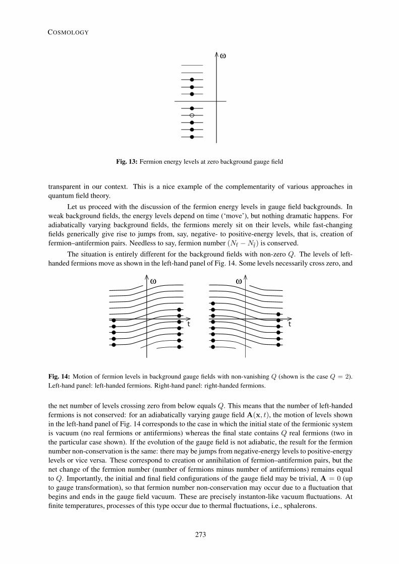
ω

Fig. 13: Fermion energy levels at zero background gauge field

transparent in our context. This is a nice example of the complementarity of various approaches inquantum field theory.

Let us proceed with the discussion of the fermion energy levels in gauge field backgrounds. Inweak background fields, the energy levels depend on time (‘move’), but nothing dramatic happens. Foradiabatically varying background fields, the fermions merely sit on their levels, while fast-changingfields generically give rise to jumps from, say, negative- to positive-energy levels, that is, creation offermion–antifermion pairs. Needless to say, fermion number (Nf −Nf) is conserved.

The situation is entirely different for the background fields with non-zero Q. The levels of left-handed fermions move as shown in the left-hand panel of Fig. 14. Some levels necessarily cross zero, and

ω

t

ω

t

Fig. 14: Motion of fermion levels in background gauge fields with non-vanishing Q (shown is the case Q = 2).Left-hand panel: left-handed fermions. Right-hand panel: right-handed fermions.

the net number of levels crossing zero from below equals Q. This means that the number of left-handedfermions is not conserved: for an adiabatically varying gauge field A(x, t), the motion of levels shownin the left-hand panel of Fig. 14 corresponds to the case in which the initial state of the fermionic systemis vacuum (no real fermions or antifermions) whereas the final state contains Q real fermions (two inthe particular case shown). If the evolution of the gauge field is not adiabatic, the result for the fermionnumber non-conservation is the same: there may be jumps from negative-energy levels to positive-energylevels or vice versa. These correspond to creation or annihilation of fermion–antifermion pairs, but thenet change of the fermion number (number of fermions minus number of antifermions) remains equalto Q. Importantly, the initial and final field configurations of the gauge field may be trivial, A = 0 (upto gauge transformation), so that fermion number non-conservation may occur due to a fluctuation thatbegins and ends in the gauge field vacuum. These are precisely instanton-like vacuum fluctuations. Atfinite temperatures, processes of this type occur due to thermal fluctuations, i.e., sphalerons.

35

COSMOLOGY

273

If the same gauge field interacts also with right-handed fermions, the motion of the levels of thelatter is opposite to that of left-handed fermions. This is shown in the right-hand panel of Fig. 14.The change in the number of right-handed fermions is equal to −Q. So, if the gauge interaction isvector-like, the total fermion number (Nleft + Nright) is conserved, while chirality (Nleft − Nright) isviolated even for massless fermions. This explains why there is no baryon number violation in QCD.The above discussion implies, instead, that there is non-perturbative violation of chirality in QCD inthe limit of massless quarks. The latter phenomenon has non-trivial consequences, which are indeedconfirmed by phenomenology. In this sense anomalous non-conservation of fermion quantum numbersis an experimentally established fact.

In electroweak theory, right-handed fermions do not interact with the SU(2)W gauge field, whileleft-handed fermions do. Therefore, fermion number is not conserved (the anomalous relations (75) and(76) suggest that this result is valid also in the presence of the Standard Model Yukawa couplings ofquarks and leptons; this is indeed the case). Since fermions of each SU(2)W doublet interact with theSU(2)W gauge bosons in one and the same way, they are equally created in a process involving a gaugefield fluctuation with non-zero Q. This again leads to the relations (77) and (78), i.e., to the selectionrules ∆B = ∆L and ∆Le = ∆Lµ = ∆Lτ .

5.3 Electroweak baryogenesisIt is tempting to make use of the electroweak mechanism of baryon number non-conservation for ex-plaining the baryon asymmetry of the Universe. This scenario is known as electroweak baryogenesis. Itmeets two problems, however. One is that CP-violation in the Standard Model is too weak: the CKMmechanism alone is insufficient to generate a realistic value of the baryon asymmetry. Hence, one needsextra sources of CP-violation. Another problem has to do with departure from thermal equilibrium that isnecessary for the generation of the baryon asymmetry. At temperatures well above 100 GeV, electroweaksymmetry is restored, the expectation value of the Englert–Brout–Higgs field φ is zero, the relation (79)is valid and the baryon number non-conservation is rapid as compared to the cosmological expansion. Attemperatures of order 100 GeV, the relation (79) may be violated, but the Universe expands very slowly:the cosmological time-scale at these temperatures is

H−1 =M∗Pl

T 2∼ 10−10 s , (80)

which is very large by the electroweak physics standards. The only way in which a strong departure fromthermal equilibrium at these temperatures may occur appears to be the first-order phase transition.

The property that at temperatures well above 100 GeV the expectation value of the Englert–Brout–Higgs field is zero, while it is non-zero in vacuo, suggests that there may be a phase transition from thephase with 〈φ〉 = 0 to the phase with 〈φ〉 6= 0. The situation is pretty subtle here, as φ is not gaugeinvariant and hence cannot serve as an order parameter, so the notion of phases with 〈φ〉 = 0 and〈φ〉 6= 0 is vague. In fact, neither electroweak theory nor most of its extensions have a gauge-invariantorder parameter, so there is no real distinction between these ‘phases’. This situation is similar to that in aliquid–vapour system, which does not have an order parameter and may or may not experience a vapour–liquid phase transition as temperature decreases, depending on other, external parameters characterizingthis system, e.g., pressure. In the Standard Model the role of such an ‘external’ parameter is played bythe Englert–Brout–Higgs self-coupling λ or, in other words, the Higgs boson mass.

Continuing to use somewhat sloppy terminology, we recall that in thermal equilibrium any systemis at the global minimum of its free energy. To figure out the expectation value of φ at a given temperature,one introduces the temperature-dependent effective potential Veff(φ;T ), which is equal to the free energydensity in the system where the average field is pinpointed to a prescribed value φ, but otherwise there isthermal equilibrium. Then the global minimum of Veff at a given temperature is at the equilibrium valueof φ, while local minima correspond to metastable states.

36

V. RUBAKOV

274

Veff(φ) Veff(φ)

φ φ

Fig. 15: Effective potential as function of φ at different temperatures. Left: first-order phase transition. Right:second-order phase transition. Upper curves correspond to higher temperatures. Black blobs show the expectationvalue of φ in thermal equilibrium. The arrow in the left-hand panel illustrates the transition from the metastable,supercooled state to the ground state.

The interesting case for us is the first-order phase transition. In this case, the system evolves asfollows. At high temperatures, there exists one minimum of Veff at φ = 0, and the expectation value of theEnglert–Brout–Higgs field is zero. As the temperature decreases, another minimum appears at finite φ,and then becomes lower than the minimum at φ = 0; see left-hand panel of Fig. 15. However, the minimawith φ = 0 and φ 6= 0 are separated by a barrier of Veff , the probability of the transition from the phaseφ = 0 to the phase φ 6= 0 is very small for some time and the system gets overcooled. The transitionoccurs when the temperature becomes sufficiently low and the transition probability sufficiently high.This is to be contrasted to the case, e.g., of the second-order phase transition, right-hand panel of Fig. 15.In the latter case, the field slowly evolves, as the temperature decreases, from zero to non-zero vacuumvalue, and the system remains very close to thermal equilibrium at all times.

During the first-order phase transition, the field cannot jump from φ = 0 to φ 6= 0 homogeneouslythroughout the whole space: intermediate homogeneous configurations have free energies proportionalto the volume of the system (recall that Veff is free energy density), i.e., infinite. Instead, the transitionoccurs just like the first-order vapour–liquid transition, through boiling. Thermal fluctuations sponta-neously create bubbles of the new phase inside the old phase. These bubbles then grow, their wallseventually collide and the new phase finally occupies the entire space. The Universe boils. In the cos-mological context, this process happens when the bubble nucleation rate per Hubble time per Hubblevolume is roughly of order 1, i.e., when a few bubbles are created in Hubble volume in Hubble time. Thevelocity of the bubble wall in the relativistic cosmic plasma is roughly of the order of the speed of light(in fact, it is somewhat smaller, from 0.1 to 0.01), simply because there are no relevant dimensionlessparameters characterizing the system. Hence, the bubbles grow large before their walls collide: their sizeat collision is roughly of the order of the Hubble size (in fact, one or two orders of magnitude smaller).While the bubble is microscopic at nucleation—its size is determined by the electroweak scale and isroughly of order (100 GeV)−1 ∼ 10−16 cm—its size at collision of walls is macroscopic, R ∼ 10−2–10−3 cm, as follows from (80). Clearly, boiling is a highly non-equilibrium process, and one may hopethat the baryon asymmetry may be generated at that time. And, indeed, there exist mechanisms of thegeneration of the baryon asymmetry, which have to do with interactions of quarks and leptons with mov-ing bubble walls. The value of the resulting baryon asymmetry may well be of order 10−10, as requiredby observations, provided that there is enough CP-violation in the theory.

A necessary condition for the electroweak generation of the baryon asymmetry is that the inequal-ity (79) must be violated just after the phase transition. Indeed, in the opposite case the electroweak

37

COSMOLOGY

275

baryon number violating processes are fast after the transition, and the baryon asymmetry, generatedduring the transition, is washed out afterwards. Hence, the phase transition must be of strong enoughfirst order. This is not the case in the Standard Model. To see why this is so, and to get an idea of inwhich extensions of the Standard Model the phase transition may be of strong enough first order, let usconsider the effective potential in some detail. At zero temperature, the Englert–Brout–Higgs potentialhas the standard form,

V (φ) = −m2

2|φ|2 +

λ

4|φ|4 .

Here

|φ| ≡(φ†φ)1/2

(81)

is the length of the Englert–Brout–Higgs doublet φ, m2 = λv2 and v = 246 GeV is the Englert–Brout–Higgs expectation value in vacuo. The Higgs boson mass is related to the latter as follows:

mH =√

2λv . (82)

Now, to the leading order of perturbation theory, the finite-temperature effects modify the effective po-tential into

Veff(φ, T ) =α(T )

2|φ|2 − β

3T |φ|3 +

λ

4|φ|4 . (83)

Here α(T ) = −m2 + g2T 2, where g2 is a positive linear combination of squares of coupling constantsof all fields to the Englert–Brout–Higgs field (in the Standard Model, a linear combination of g2, g′ 2 andy2i , where g and g′ are SU(2)W and U(1)Y gauge couplings and yi are Yukawa couplings). The phase

transition occurs roughly when α(T ) = 0. An important parameter β is a positive linear combinationof cubes of coupling constants of all bosonic fields to the Englert–Brout–Higgs field. In the StandardModel, β is a linear combination of g3 and g′ 3, i.e., a linear combination of M3

W/v3 and M3

Z/v3,

β =1

2π

2M3W +M3

Z

v3. (84)

The cubic term in (83) is rather peculiar: in view of (81), it is not analytic in the original Englert–Brout–Higgs field φ. Yet this term is crucial for the first-order phase transition: for β = 0 the phase transitionwould be of the second order.

Question. Show that the phase transition is second order for β = 0.

The origin of the non-analytic cubic term can be traced back to the enhancement of the Bose–Einstein thermal distribution at low momenta, p,m T ,

fBose(p) =1

e

√p2+m2

aT − 1

' T√p2 +m2

a

,

where m ' ga|φ| is the mass of the boson a that is generated due to the non-vanishing Englert–Brout–Higgs field, and ga is the coupling constant of the field a to the Englert–Brout–Higgs field. Clearly, atp g|φ| the distribution function is non-analytic in φ,

fBose(p) 'T

ga|φ|.

It is this non-analyticity that gives rise to the non-analytic cubic term in the effective potential. Impor-tantly, the Fermi–Dirac distribution,

fFermi(p) =1

e

√p2+m2

aT + 1

,

38

V. RUBAKOV

276

is analytic in m2a, and hence φ†φ, so fermions do not contribute to the cubic term.

With the cubic term in the effective potential, the phase transition is indeed of the first order:at high temperatures the coefficient α is positive and large, and there is one minimum of the effectivepotential at φ = 0, while for α small but still positive there are two minima. The phase transition occursat α ≈ 0; at that moment

Veff(φ, T ) ≈ −βT3|φ|3 +

λ

4|φ|4 .

We find from this expression that immediately after the phase transition the minimum of Veff is at

φ ' βT

λ.

Hence, the necessary condition for successful electroweak baryogenesis, φ > T , translates into

β > λ . (85)

According to (82), λ is proportional to m2H, whereas in the Standard Model β is proportional to (2M3

W +M3

Z). Therefore, the relation (85) holds for small Higgs boson masses only; in the Standard Model onemakes use of (82) and (84) and finds that this happens formH < 50 GeV, while in realitymH = 125 GeV.In fact, in the Standard Model with mH = 125 GeV, there is no phase transition at all; the electroweaktransition is a smooth crossover instead. The latter fact is not visible from the expression (83), but thatexpression is the lowest-order perturbative result, while the perturbation theory is not applicable fordescribing the transition in the Standard Model with large mH.

This discussion indicates a possible way to make the electroweak phase transition strong. Whatone needs is the existence of new bosonic fields that have large enough couplings to the Englert–Brout–Higgs field(s), and hence provide large contributions to β. To have an effect on the dynamics of thetransition, the new bosons must be present in the cosmic plasma at the transition temperature, T ∼100 GeV, so their masses should not be too high, M . 300 GeV. In supersymmetric extensions of theStandard Model, the natural candidate for a long time has been stop (superpartner of top-quark) whoseYukawa coupling to the Englert–Brout–Higgs field is the same as that of top, that is, large. The light stopscenario for electroweak baryogenesis would indeed work, as has been shown by the detailed analysis inRefs. [68–70].

There are other possibilities to make the electroweak transition strongly first order. Generically,they require an extension of the scalar sector of the Standard Model and predict new fairly light scalarswhich interact with the Standard Model Englert–Brout–Higgs field and may or may not participate ingauge interactions.

Yet another issue is CP-violation, which has to be strong enough for successful electroweak baryo-genesis. As the asymmetry is generated in the interactions of quarks and leptons with the bubble walls,CP-violation must occur at the walls. Recall now that the walls are made of the scalar field(s). Thispoints towards the necessity of CP-violation in the scalar sector, which may only be the case in a theorycontaining scalar fields other than the Standard Model Englert–Brout–Higgs field.

To summarize, electroweak baryogenesis requires a considerable extension of the Standard Model,with masses of new particles in the range 100–300 GeV. Hence, this mechanism will most likely be ruledout or confirmed by the LHC. We emphasize, however, that electroweak baryogenesis is not the onlyoption at all: an elegant and well-motivated competitor is leptogenesis [14, 15, 71]; there are many othermechanisms proposed in the literature.

6 Before the hot epoch6.1 Cosmological perturbations: preliminariesWith BBN theory and observations, and due to evidence, albeit indirect, for relic neutrinos, we areconfident of the theory of the early Universe at temperatures up to T ' 1 MeV, which correspond to an

39

COSMOLOGY

277

age of t ' 1 s. With the LHC, we hope to be able to learn the Universe up to temperature T ∼ 100 GeVand age t ∼ 10−10 s. Are we going to have a handle on an even earlier epoch?

The key issue in this regard is cosmological perturbations. These are inhomogeneities in the en-ergy density and associated gravitational potentials, in the first place. This type of inhomogeneities iscalled scalar perturbations, as they are described by 3-scalars. There may exist perturbations of anothertype, called tensors; these are primordial gravity waves. We will mostly concentrate on scalar perturba-tions, since they are observed; tensor perturbations are important too, and we comment on them later on.While perturbations of the present size of order 10 Mpc and smaller have large amplitudes today and arenon-linear, amplitudes of all known perturbations were small in the past, and the perturbations can be de-scribed within the linearized theory. Indeed, CMB temperature anisotropy tells us that the perturbationsat the recombination epoch were roughly at the level

δ ≡ δρ

ρ= 10−4–10−5 . (86)

Thus, the linearized theory works very well before recombination and somewhat later. We will be rathersloppy when talking about scalar perturbations. In general relativity, there is arbitrariness in the choice ofreference frame, which can be viewed as a sort of gauge freedom. In a homogeneous and isotropic Uni-verse, there is a preferred reference frame, in which quantities like energy density or distribution functionof CMB photons are manifestly homogeneous and isotropic. It is in this frame that the metric has FLRWform (1). Once there are perturbations, no preferred reference frame exists any longer. As an example,one can choose a reference frame such that the three-dimensional hypersurfaces of constant time arehypersurfaces of constant total energy density ρ. In this frame one has δρ = 0, so Eq. (86) does notmake sense. Yet the Universe is inhomogeneous in this reference frame, since there are inhomogeneousmetric perturbations δgµν(x, t). We will skip these technicalities and denote the scalar perturbation by δwithout specifying its gauge-invariant meaning.

Equations for perturbations are obtained by writing for every variable (including metric) an ex-pression like ρ(x, t) = ρ(t) + δρ(x, t) etc, where ρ(t) is the homogeneous and isotropic background,which we discussed in Section 2.3. One inserts the perturbed variables into the Einstein equations andcovariant conservation equations ∇µTµν = 0 and linearizes this set of equations. In many cases onealso has to use the linearized Boltzmann equations that govern the distribution functions of particles outof thermal equilibrium; these are necessary for evaluating the linearized perturbations of the energy–momentum tensor. In any case, since the background FLRW metric (1) does not explicitly depend on x,the linearized equations for perturbations do not contain x explicitly. Therefore, one makes use of thespatial Fourier decomposition

δ(x, t) =

∫eikxδ(k, t) d3k .

The advantage is that modes with different momenta k evolve independently in the linearized theory, i.e.,each mode can be treated separately. Recall that dx is not the physical distance between neighbouringpoints; the physical distance is a(t)dx. Thus, k is not the physical momentum (wavenumber); thephysical momentum is k/a(t). While for a given mode the comoving (or coordinate) momentum kremains constant in time, the physical momentum gets red shifted as the Universe expands, see alsoSection 2.1. In what follows we set the present value of the scale factor equal to 1 (in a spatially flatUniverse this can always be done by rescaling the coordinates x):

a0 ≡ a(t0) = 1 ;

then k is the present physical momentum and 2π/k is the present physical wavelength, which is alsocalled the comoving wavelength.

Properties of scalar perturbations are measured in various ways. Perturbations of fairly largespatial scales (fairly low k) give rise to CMB temperature anisotropy and polarization, so we have very

40

V. RUBAKOV

278

detailed knowledge of them. Somewhat shorter wavelengths are studied by analysing distributions ofgalaxies and quasars at present and in relatively near past. There are several other methods, some ofwhich can probe even shorter wavelengths. There is good overall consistency of the results obtained bydifferent methods, so we have a pretty good understanding of many aspects of the scalar perturbations.

The cosmic medium in our Universe has several components that interact only gravitationally:baryons, photons, neutrinos and dark matter. Hence, there may be and, in fact, there are perturbations ineach of these components. As we pointed out in Section 4, electromagnetic interactions between baryons,electrons and photons were strong before recombination, so to a reasonable approximation these speciesmade a single fluid, and it is appropriate to talk about perturbations in this fluid. After recombination,baryons and photons evolved independently.

By studying the scalar perturbations, we have learned a number of very important things. Toappreciate what they are, it is instructive to consider first the baryon–electron–photon fluid before re-combination.

6.2 Perturbations in the expanding Universe: subhorizon and superhorizon regimes.Perturbations in the baryon–photon fluid before recombination are nothing but sound waves. It is in-structive to compare the wavelength of a perturbation with the horizon size. To this end, recall (seeSection 2.4) that the horizon size lH(t) is the size of the largest region which is causally connected bythe time t, and that

lH(t) ∼ H−1(t) ∼ tat radiation domination and later, see Eq. (21). The latter relation, however, holds under the assumptionthat the hot epoch was the first one in cosmology, i.e., that the radiation domination started right after theBig Bang. This assumption is in the heart of what can be called hot Big Bang theory. We will find thatthis assumption in fact is not valid for our Universe; we are going to see this ad absurdum, so let us stickto the hot Big Bang theory for the time being.

Unlike the horizon size, the physical wavelength of a perturbation grows more slowly. As anexample, at radiation domination

λ(t) =2πa(t)

k∝√t ,

while at matter domination λ(t) ∝ t2/3. For obvious reasons, the modes with λ(t) H−1(t) andλ(t) H−1(t) are called subhorizon and superhorizon at time t, respectively. We are able to studythe modes which are subhorizon today; longer modes are homogeneous throughout the visible Universeand are not observed as perturbations. However, the wavelengths which are subhorizon today weresuperhorizon at some earlier epoch. In other words, the physical momentum k/a(t) was smaller thanH(t) at early times; at time t× such that

q(t×) ≡ k

a(t×)= H(t×) ,

the mode entered the horizon, and after that evolved in the subhorizon regime k/a(t) H(t), seeFig. 16. It is straightforward to see that for all cosmologically interesting wavelengths, horizon crossingoccurs much later than 1 s after the Big Bang, i.e., at the time we are confident about. So, there is noguesswork at this point.

Question. Estimate the temperature at which a perturbation of comoving size 10 kpc entered the horizon.

Another way to look at the superhorizon–subhorizon behaviour of perturbations is to introduce a

41

COSMOLOGY

279

t

q2(t) q1(t) = k1/a(t)

H(t)

t×

Fig. 16: Physical momenta q(t) = k/a(t) (solid lines, k2 < k1) and Hubble parameter (dashed line) at radiation-and matter-dominated epochs. Here t× is the horizon entry time.

new time coordinate (cf. Eq. (20)),

η =

∫ t

0

dt′

a(t′). (87)

Note that this integral converges at the lower limit in the hot Big Bang theory. In terms of this timecoordinate, the FLRW metric (1) reads

ds2 = a2(η)(dη2 − dx2) .

In coordinates (η,x), the light cones ds = 0 are the same as in Minkowski space, and η is the coordinatesize of the horizon, see Fig. 17.

Every mode of perturbation has a time-independent coordinate wavelength 2π/k, and at small ηit is in superhorizon regime, 2π/k η, and after horizon crossing at time η× = η(t×) it becomessubhorizon.

Fig. 17: Causal structure of space–time in the hot Big Bang theory. Here tr is the conformal time at recombination.

42

V. RUBAKOV

280

6.3 Hot epoch was not the firstOne immediately observes that this picture falsifies the hot Big Bang theory. Indeed, we see the horizonat recombination lH(trec) at an angle ∆θ ≈ 2, as schematically shown in Fig. 17. By causality, at re-combination there should be no perturbations of larger wavelengths, as any perturbation can be generatedwithin the causal light cone only. In other words, CMB temperature must be isotropic when averagedover angular scales exceeding 2; there should be no cold or warm spots of angular size larger than 2.Now, CMB provides us with the photographic picture shown in Fig. 18. It is seen by the naked eye that

Fig. 18: CMB sky as seen by Planck

there are cold and warm regions whose angular size much exceeds 2; in fact, there are perturbationsof all angular sizes up to those comparable to the entire sky. We come to an important conclusion: thescalar perturbations were built in at the very beginning of the hot epoch. The hot epoch was not the first,it was preceded by some other epoch, and the cosmological perturbations were generated then.

Question. Assuming (erroneously) that there is no dark energy, and that recombination occurred deep inthe matter-dominated epoch, estimate the angular scale of the horizon at recombination.

Another manifestation of the fact that the scalar perturbations were there already at the beginningof the hot epoch is the existence of peaks in the angular spectrum of CMB temperature. In general,perturbations in the baryon–photon medium before recombination are acoustic waves,

δ(k, t) = δ(k)eikx cos

[∫ t

0vs

k

a(t′)dt′ + ψk

], (88)

where vs is sound speed, δ(k) is time-independent amplitude and ψk is time-independent phase. Thisexpression is valid, however, in the subhorizon regime only, i.e., at late times. The two solutions insuperhorizon regime at radiation domination are

δ(t) = const , (89a)

δ(t) =constt3/2

. (89b)

Were the perturbations generated in a causal way at radiation domination, they would be always subhori-zon. In that case the solutions (89) would be irrelevant, and there would be no reason for a particular

43

COSMOLOGY

281

choice of phase ψk in Eq. (88). One would rather expect that ψk is a random function of k. This isindeed the case for specific mechanisms of the generation of density perturbations at the hot epoch [72].

On the other hand, if the perturbations existed at the very beginning of the hot epoch, they weresuperhorizon at sufficiently early times, and were described by the solutions (89). The consistency ofthe whole cosmology requires that the amplitude of perturbations was small at the beginning of thehot stage. The solution (89b) rapidly decays away, and towards the horizon entry the perturbation isin constant mode (89a). So, the initial condition for the further evolution is unique modulo amplitudeδ(k), and hence the phase ψ(k) is uniquely determined. For modes that enter the horizon at radiationdomination this phase is equal to zero and, after entering the horizon, the modes oscillate as follows:

δ(k, t) = δ(k)eikx cos

[∫ t

0vs

k

a(t′)dt′].

At recombination, the perturbation is

δ(k, tr) = δ(k)eikx cos(krs) , (90)

where

rs =

∫ trec

0vs

dt′

a(t′)

is the comoving size of the sound horizon at recombination, while its physical size equals a(trec)rs.So, we see that the density perturbation of the baryon–photon plasma at recombination oscillates as afunction of wavenumber k. The period of this oscillation is determined by rs, which is a straightforwardlycalculable quantity.

So, if the perturbations existed already at the beginning of the hot stage, they show the oscillatorybehaviour in momentum at the recombination epoch. This translates into an oscillatory pattern of theCMB temperature angular spectrum. Omitting details, the fluctuation of the CMB temperature is partiallydue to the density perturbation in the baryon–photon medium at recombination. Namely, the temperaturefluctuation of photons coming from the direction n in the sky is, roughly speaking,

δT (n) ∝ δγ(xn, ηrec) + δTsmooth(n) ,

where Tsmooth(n) corresponds to the non-oscillatory part of the CMB angular spectrum and

xn = −n(η0 − ηrec) .

Here (η0−ηrec) is the coordinate distance to the sphere of photon last scattering, and xn is the coordinateof the place where the photons coming from the direction n scatter the last time. The quantity Tsmooth(n)originates from the gravitational potential generated by the dark matter perturbation; dark matter haszero pressure at all times, so there are no sound waves in this component, and there are no oscillations atrecombination as a function of momentum.

One expands the temperature variation on the celestial sphere in spherical harmonics:

δT (n) =∑

lm

almYlm(θ, φ).

The multipole number l characterizes the temperature fluctuations at the angular scale ∆θ = π/l. Thesound waves of momentum k are seen roughly at an angle ∆θ = ∆x/(η0 − ηrec), where ∆x = π/k isthe coordinate half-wavelength. Hence, there is the correspondence

l←→ k(η0 − ηrec) .

44

V. RUBAKOV

282

Fig. 19: The angular spectrum of the CMB temperature anisotropy [73]. The quantity on the vertical axis is Dl

defined in (92). Note the unconventional scale on the horizontal axis, aimed at showing both small-l region (largeangular scales) and large-l region.

Oscillations in momenta in Eq. (90) thus translate into oscillations in l, and these are indeed observed,see Fig. 19.

To understand what is shown in Fig. 19, we note that all observations today support the hypothesisthat alm are independent Gaussian random variables. For a hypothetical ensemble of Universes likeours, the average values of products of the coefficients alm would obey

〈alma∗l′m′〉 = Clδll′δmm′ . (91)

This gives the expression for the temperature fluctuation:

〈[δT (n)]2〉 =∑

l

2l + 1

4πCl ≈

∫dl

lDl ,

where

Dl =l(l + 1)

2πCl . (92)

Of course, one cannot measure the ensemble average (91). The definition of Cl used in experiments is

Cl =1

2l + 1

l∑

m=−l|alm|2 ,

where alm are measured quantities. Since we have only one Universe, this is generically different fromthe ensemble average (91): for given l, there are only 2l + 1 measurements, and the intrinsic statisticaluncertainty—cosmic variance—is of order (2l + 1)−1/2. It is this uncertainty, rather than experimentalerror, that is shown in Fig. 19.

We conclude that the facts that the CMB angular spectrum has oscillatory behaviour and that thereare sizeable temperature fluctuations at l < 50 (angular scale greater than the angular size of 2 of thehorizon at recombination) unambiguously tell us that the density perturbations were indeed superhorizonat the hot cosmological stage. The hot epoch has to be preceded by some other epoch—the epoch of thegeneration of perturbations.

45

COSMOLOGY

283

6.4 Primordial scalar perturbationsThere are several things which we already know about the primordial density perturbations. By ‘pri-mordial’ we mean the perturbations deep in the superhorizon regime at the radiation-domination epoch.As we already know, perturbations are time-independent in this regime, see Eq. (89a). They set the ini-tial conditions for further evolution, and this evolution is well understood, at least in the linear regime.Hence, using observational data, one is able to measure the properties of primordial perturbations. Ofcourse, since the properties we know of are established by observations, they are valid within certain errorbars. Conversely, deviations from the results listed below, if observed, would be extremely interesting.

First, density perturbations are adiabatic. This means that there are perturbations in the energydensity, but not in composition. More precisely, the baryon-to-entropy ratio and dark matter-to-entropyratio are constant in space,

δ(nB

s

)= const , δ

(nDM

s

)= const . (93)

This is consistent with the generation of the baryon asymmetry and dark matter at the hot cosmologicalepoch: in that case, all particles were at thermal equilibrium early at the hot epoch, the temperaturecompletely characterized the whole cosmic medium at that time and as long as physics behind the baryonasymmetry and dark matter generation is the same everywhere in the Universe, the baryon and darkmatter abundances (relative to the entropy density) are necessarily the same everywhere. In principle,there may exist entropy (another term is isocurvature) perturbations, such that at the early hot epochenergy density (dominated by relativistic matter) was homogeneous, while the composition was not.This would give initial conditions for the evolution of density perturbations, which would be entirelydifferent from those characteristic of the adiabatic perturbations. As a result, the angular spectrum ofthe CMB temperature anisotropy would be entirely different. No admixture of the entropy perturbationshas been detected so far, but it is worth emphasizing that even a small admixture will show that manypopular mechanisms for generating dark matter and/or baryon asymmetry have nothing to do with reality.One will have to think, instead, that the baryon asymmetry and/or dark matter were generated beforethe beginning of the hot stage. A notable example is the axion misalignment mechanism discussedin Section 4.4: in a latent sense, the axion dark matter exists from the very beginning in that case, andperturbations in the axion field δθ0(x) (which may be generated together with the adiabatic perturbations)would show up as entropy perturbations in dark matter.

Second, the primordial density perturbations are Gaussian random fields. Gaussianity means thatthe three-point and all odd correlation functions vanish, while the four-point function and all higher ordereven correlation functions are expressed through the two-point function via Wick’s theorem:

〈δ(k1)δ(k2)δ(k3)〉 = 0,

〈δ(k1)δ(k2)δ(k3)δ(k4)〉 = 〈δ(k1)δ(k2)〉 · 〈δ(k3)δ(k4)〉+ permutations of momenta .

We note that this property is characteristic of vacuum fluctuations of non-interacting (linear) quantumfields. Hence, it is quite likely that the density perturbations originate from the enhanced vacuum fluctu-ations of non-interacting or weakly interacting quantum field(s). The free quantum field has the generalform

φ(x, t) =

∫d3ke−ikx

(f

(+)k (t)a†k + eikxf

(−)k (t)ak

),

where a†k and ak are creation and annihilation operators. For the field in Minkowski space–time, one hasf

(±)k (t) = e±iωkt, while enhancement, e.g., due to the evolution in time-dependent background, means

that f (±)k are large. But, in any case, Wick’s theorem is valid, provided that the state of the system is

vacuum, ak|0〉 = 0.

46

V. RUBAKOV

284

We note in passing that non-Gaussianity is an important topic of current research. It would showup as a deviation from Wick’s theorem. As an example, the three-point function (bispectrum) may benon-vanishing,

〈δ(k1)δ(k2)δ(k3)〉 = δ(k1 + k2 + k3) G(k2i ; k1k2; k1k3) 6= 0 .

The functional dependence of G(k2i ; k1k2; k1k3) on its arguments is different in different models

of generation of primordial perturbations, so this shape is a potential discriminator. In some models thebispectrum vanishes, e.g., due to symmetries. In that case the trispectrum (connected four-point function)may be measurable instead. It is worth emphasizing that non-Gaussianity has not been detected yet.

Another important property is that the primordial power spectrum of density perturbations isnearly, but not exactly, flat. For a homogeneous and anisotropic Gaussian random field, the powerspectrum completely determines its only characteristic, the two-point function. A convenient definitionis

〈δ(k)δ(k′)〉 =1

4πk3P(k)δ(k + k′) . (94)

The power spectrum P(k) defined in this way determines the fluctuation in a logarithmic interval ofmomenta,

〈δ2(x)〉 =

∫ ∞

0

dk

kP(k) .

By definition, the flat spectrum is such that P is independent of k. In this case all spatial scales are alike;no scale is enhanced with respect to another. It is worth noting that the flat spectrum was conjecturedby Harrison [74], Zeldovich [75] and Peebles and Yu [76] at the beginning of the 1970s, long beforerealistic mechanisms of the generation of density perturbations have been proposed.

In view of the approximate flatness, a natural parametrization is

P(k) = As

(k

k∗

)ns−1

, (95)

where As is the amplitude, ns− 1 is the tilt and k∗ is a fiducial momentum, chosen at one’s convenience.The flat spectrum in this parametrization has ns = 1. This is inconsistent with the cosmological data,which give [21]

ns = 0.968± 0.06 .

This quantifies what we mean by a nearly, but not exactly flat, power spectrum.

6.5 Inflation or not?The pre-hot epoch must be long in terms of the time variable η introduced in Eq. (87). What we wouldlike to have is that a large part of the Universe (e.g., the entire visible part) be causally connected towardsthe end of that epoch, see Fig. 20. A long duration in η does not necessarily mean a long duration inphysical time t; in fact, the physical duration of the pre-hot epoch may be tiny.

An excellent hypothesis on the pre-hot stage is inflation, the epoch of nearly exponential expan-sion [77–82],

a(t) = e∫Hdt , H ≈ const .

Inflation makes the whole visible Universe, and likely a much greater region of space, causally connectedat very early times. The horizon size at inflation is at least

lH(t) = a(t)

∫ t

ti

dt′

a(t′)= H−1eH(t−ti) ,

47

COSMOLOGY

285

Fig. 20: Causal structure of space–time in the real Universe

where ti is the time inflation begins, and we set H = const for illustrational purposes. This size is hugefor t− ti H−1, as desired.

Question. Assuming that at inflation H MPl, show that if the duration of inflation ∆t is larger than100H−1, the whole visible Universe is causally connected by the end of inflation. What is 100H−1 inseconds for H = 1015 GeV? Using the time variable η, show that the causal structure of space–time ininflationary theory with ∆t > 100H−1 is the one shown in Fig. 20.

From the viewpoint of perturbations, the physical momentum q(t) = k/a(t) decreases (gets redshifted) at inflation, while the Hubble parameter stays almost constant. So, every mode is first subhorizon(q(t) H(t)) and later superhorizon (q(t) H(t)). This situation is opposite to what happens atradiation and matter domination, see Fig. 21; this is precisely the prerequisite for generating the densityperturbations. In fact, inflation does generate primordial density perturbations [83–87] whose propertiesare consistent with everything we know about them. Indeed, at the inflationary epoch, fluctuations of all

inflation RD, MD epochs

H(t)

q(t)= a(t)k

tte

insidehorizon

insidehorizon

outsidehorizon

Fig. 21: Physical momentum and Hubble parameter at inflation and later: te is the time of the inflation end

48

V. RUBAKOV

286

light fields get enhanced greatly due to the fast expansion of the Universe. This is true, in particular, forthe field that dominates the energy density at inflation, called an inflaton. Enhanced vacuum fluctuationsof the inflaton are nothing but perturbations in the energy density at the inflationary epoch, which arereprocessed into perturbations in the hot medium after the end of inflation. The inflaton field is veryweakly coupled, so the non-Gaussianity in the primordial scalar perturbations is very small [88]. In fact,it is so small that its detection is problematic even in the distant future.

The approximate flatness of the primordial power spectrum in inflationary theory is explained bythe symmetry of the de Sitter space–time, which is the space–time of constant Hubble rate,

ds2 = dt2 − e2Htdx2 , H = const .

This metric is invariant under spatial dilatations supplemented by time translations,

x→ λx , t→ t− 1

2Hlog λ .

Therefore, all spatial scales are alike, which is also a defining property of the flat power spectrum. Atinflation, H is almost constant in time and the de Sitter symmetry is an approximate symmetry. For thisreason, inflation automatically generates a nearly flat power spectrum.

The distinguishing property of inflation is the generation of tensor modes (primordial gravitywaves) of sizeable amplitude and nearly flat power spectrum. The gravity waves are thus a smoking gunfor inflation. The reason for their generation at inflation is that the exponential expansion of the Universeenhances vacuum fluctuations of all fields, including the gravitational field itself. Particularly interestingare gravity waves whose present wavelengths are huge, 100 Mpc and larger. Many inflationary modelspredict their amplitudes to be very large, of order 10−6 or so. Shorter gravity waves are generated too,but their amplitudes decay after horizon entry at radiation domination, and today they have much smalleramplitudes making them inaccessible to gravity wave detectors like LIGO or VIRGO, pulsar timingarrays etc. A conventional characteristic of the amplitude of primordial gravity waves is the tensor-to-scalar ratio

r =PT

P ,

where P is the scalar power spectrum defined in Eq. (94) and PT is the tensor power spectrum definedin a similar way, but for transverse traceless metric perturbations hij . The result of the search for effectsof the tensor modes on CMB temperature anisotropy is shown in Fig. 22. This search has already ruledout some of the popular inflationary models.

All the above referred to the simplest, single-field inflationary models. In models with morethan one relevant field, the situation may be different. In particular, sizeable non-Gaussianity may begenerated, while the amplitude of tensor perturbations may be very low. So, it would be rather difficultto rule out the inflationary scenario as a whole.

Inflation is not the only hypothesis proposed so far. One option is the bouncing Universe scenario,which assumes that the cosmological evolution begins from contraction, then the contracting stage termi-nates at some moment of time (bounce) and is followed by expansion. A version is the cycling Universescenario with many cycles of contraction–bounce–expansion. See reviews by Lehners and Branden-berger in Ref. [16–20]. Another scenario is that the Universe starts out from a nearly flat and static statewith nearly vanishing energy density. Then the energy density increases and, according to the Friedmannequation, the expansion speeds up. This goes under the name of the Genesis scenario [90]. Theoreticalrealizations of these scenarios are more difficult than inflation, but they are not impossible, as becameclear recently.

The generation of the density perturbations is less automatic in scenarios alternative to inflation.Similarly to inflationary theory, the flatness of the scalar power spectrum is likely to be due to somesymmetry. One candidate symmetry is conformal invariance [91–94]. The point is that the conformal

49

COSMOLOGY

287

Fig. 22: Allowed regions (at 68% and 95% confidence levels) in the plane (ns, r), where ns is the scalar spectralindex and r is the tensor-to-scalar ratio [89]. The right lower corner (the point (1.0, 0.0)) is the Harrison–Zeldovichpoint (flat scalar spectrum, no tensor modes). Intervals show predictions of popular inflationary models.

group includes dilatations, xµ → λxµ. This property indicates that the theory possesses no scale and hasa good chance for producing the flat spectrum. A model building along this direction has begun ratherrecently [92–94].

6.6 Hunt continuesUntil now, only very basic facts about the primordial cosmological perturbations have been observa-tionally established. Even though very suggestive, these facts by themselves are not sufficient to un-ambiguously figure out what was the Universe at the pre-hot epoch of its evolution. New properties ofcosmological perturbations will hopefully be discovered in the future and shed more light on this pre-hotepoch. Let us discuss some of the potential observables.

6.6.1 Tensor perturbations = relic gravity wavesAs we discussed, primordial tensor perturbations are predicted by many inflationary models. On theother hand, there seems to be no way of generating a nearly flat tensor power spectrum in alternatives toinflation. In fact, most, if not all, alternative scenarios predict unobservably small tensor amplitudes. Thisis why we said that tensor perturbations are a smoking gun for inflation. Until recently, the most sensitiveprobe of the tensor perturbations has been the CMB temperature anisotropy [95–98]. However, the mostpromising tool is the CMB polarization. The point is that a certain class of polarization patterns (calledB-mode) is generated by tensor perturbations, while scalar perturbations are unable to create it [99,100].Hence, dedicated experiments aiming at measuring the CMB polarization may well discover the tensorperturbations, i.e., relic gravity waves. Needless to say, this would be a profound discovery. To avoidconfusion, let us note that the CMB polarization has been already observed, but it belongs to anotherclass of patterns (so-called E-mode) and is consistent with the existence of the scalar perturbations only.The original claim of the BICEP-2 experiment [101] to detect the B-mode generated by primordial tensorperturbations was turned down [102]: the B-mode is there, but it is due to dust in our Galaxy.

50

V. RUBAKOV

288

6.6.2 Non-Gaussianity.As we pointed out already, non-Gaussianity of density perturbations is very small in the simplest in-flationary models. Hence, its discovery will signal that either inflation and inflationary generation ofdensity perturbations occurred in a rather complicated way, or an alternative scenario was realized. Oncethe non-Gaussianity is discovered, and its shape is revealed even with modest accuracy, many concretemodels will be ruled out, while at most a few will get strong support.

6.6.3 Statistical anisotropy.In principle, the power spectrum of density perturbations may depend on the direction of momentum,e.g.,

P(k) = P0(k)

(1 + wij(k)

kikjk2

+ · · ·),

where wij is a fundamental tensor in our part of the Universe (odd powers of ki would contradict com-mutativity of the Gaussian random field δ(k), see Eq. (94)). Such a dependence would definitely implythat the Universe was anisotropic at the pre-hot stage, when the primordial perturbations were gener-ated. This statistical anisotropy is rather hard to obtain in inflationary models, though it is possible ininflation with strong vector fields [103–105]. On the other hand, statistical anisotropy is natural in someother scenarios, including conformal models [106, 107]. The statistical anisotropy would show up incorrelators [108, 109]

〈almal′m′〉 with l′ 6= l and/or m′ 6= m.

At the moment, the constraints [110, 111] on statistical anisotropy obtained by analysing the CMB dataare getting into the region which is interesting from the viewpoint of some (though not many) models ofthe pre-hot epoch.

6.6.4 Admixture of entropy perturbations.As we explained above, even a small admixture of entropy perturbations would force us to abandon themost popular scenarios of the generation of baryon asymmetry and/or dark matter, which assumed thatit happened at the hot epoch. Once the dark matter entropy mode is discovered, the WIMP dark matterwould no longer be well motivated, while other, very weakly interacting dark matter candidates, likeaxions or superheavy relics, would be preferred. This would redirect the experimental search for darkmatter.

7 ConclusionIt is by now commonplace that the two fields studying together the most fundamental properties of matterand the Universe—particle physics and cosmology—are tightly interrelated. The present situations inthese fields have much in common too. On the particle-physics side, the Standard Model has beencompleted by the expected discovery of the Higgs boson. On the other hand, relatively recently a fairlyunexpected discovery of neutrino oscillations was made, which revolutionized our view on particles andtheir interactions. There are grounds to hope for even more profound discoveries, notably by the LHCexperiments. While in the past there were definite predictions of the Standard Model, which eventuallywere confirmed, there are numerous hypotheses concerning new physics, none of which is undoubtedlyplausible. On the cosmology side, the Standard Model of cosmology, ΛCDM, has been shaped, againnot without an unexpected and revolutionary discovery, in this case of the accelerated expansion of theUniverse. We hope for further profound discoveries in cosmology too. It may well be that we willsoon learn which is the dark matter particle; again, there is an entire zoo of candidates, several of whichare serious competitors. The discoveries of new properties of cosmological perturbations will hopefullyreveal the nature of the pre-hot epoch. There is a clear best guess, inflation, but it is not excluded thatfuture observational data will point towards something else.

51

COSMOLOGY

289

Neither in particle physics nor in cosmology are new discoveries guaranteed, however. Naturemay hide its secrets. Whether or not it does is the biggest open issue in fundamental physics.

AcknowledgementThis work is supported by the Russian Science Foundation grant 14-22-00161.

References[1] S. Dodelson, Modern Cosmology (Academic Press, Amsterdam, 2003).[2] V. Mukhanov, Physical Foundations of Cosmology (Cambridge University Press, Cambridge,

2005). http://dx.doi.org/10.1017/CBO9780511790553[3] S. Weinberg, Cosmology (Oxford University Press, Oxford, 2008).[4] A.R. Liddle and D.H. Lyth, The Primordial Density Perturbation: Cosmology, Inflation and the

Origin of Structure (Cambridge University Press, Cambridge, 2009).http://dx.doi.org/10.1017/CBO9780511819209

[5] D.S. Gorbunov and V.A. Rubakov, Introduction to the Theory of the Early Universe: Hot BigBang Theory (World Scientific, Hackensack, NJ, 2011). http://dx.doi.org/10.1142/7874

[6] D.S. Gorbunov and V.A. Rubakov, Introduction to the Theory of the Early Universe:Cosmological Perturbations and Inflationary Theory (World Scientific, Hackensack, NJ, 2011).http://dx.doi.org/10.1142/7874

[7] K.A. Olive, arXiv:astro-ph/0301505.[8] G. Bertone, D. Hooper and J. Silk, Phys. Rep. 405(5–6) (2005) 279.

http://dx.doi.org/10.1016/j.physrep.2004.08.031[9] A. Boyarsky, O. Ruchayskiy and M. Shaposhnikov, Annu. Rev. Nucl. Part. Sci. 59 (2009) 191.

http://dx.doi.org/10.1146/annurev.nucl.010909.083654[10] M. Kawasaki and K. Nakayama, Annu. Rev. Nucl. Part. Sci. 63 (2013) 69.

http://dx.doi.org/10.1146/annurev-nucl-102212-170536[11] V.A. Rubakov and M.E. Shaposhnikov, Usp. Fiz. Nauk 166 (1996) 493 [Engl. Trans. Phys. Usp.

39 (1996) 461]. http://dx.doi.org/10.3367/UFNr.0166.199605d.0493[12] M. Trodden, Rev. Mod. Phys. 71(5) (1999) 1463. http://dx.doi.org/10.1103/RevModPhys.71.1463[13] T. Konstandin, Usp. Fiz. Nauk 183 (2013) 785 [Engl. trans. Phys. Usp. 56 (2013) 747].

http://dx.doi.org/10.3367/UFNr.0183.201308a.0785[14] W. Buchmuller, R.D. Peccei and T. Yanagida, Annu. Rev. Nucl. Part. Sci. 55 (2005) 311.

http://dx.doi.org/10.1146/annurev.nucl.55.090704.151558[15] S. Davidson, E. Nardi and Y. Nir, Phys. Rep. 466(4–5) (2008) 105.

http://dx.doi.org/10.1016/j.physrep.2008.06.002[16] D.H. Lyth and A. Riotto, Phys. Rep. 314(1–2) (1999) 16.

http://dx.doi.org/10.1016/S0370-1573(98)00128-8[17] B.A. Bassett, S. Tsujikawa and D. Wands, Rev. Mod. Phys. 78(2) (2006) 537.

http://dx.doi.org/10.1103/RevModPhys.78.537[18] J.L. Lehners, Phys. Rep. 465(6) (2008) 223-263. http://dx.doi.org/10.1016/j.physrep.2008.06.001[19] A. Mazumdar and J. Rocher, Phys. Rep. 497(4–5) (2011) 85.

http://dx.doi.org/10.1016/j.physrep.2010.08.001[20] R.H. Brandenberger, Lect. Notes Phys. 863 (2013) 333.

http://dx.doi.org/10.1007/978-3-642-33036-0_12[21] P.A.R. Ade et al. (Planck Collaboration), arXiv:1502.01589 [astro-ph.CO].

52

V. RUBAKOV

290

[22] P.A.R. Ade et al. (Planck Collaboration), Astron. Astrophys. 571 (2014) A16.http://dx.doi.org/10.1051/0004-6361/201321591

[23] E. Gawiser and J. Silk, Phys. Rep. 333 (2000) 245.http://dx.doi.org/10.1016/S0370-1573(00)00025-9

[24] K. Hagiwara et al. (Particle Data Group Collaboration), Phys. Rev. D 66(1) (2002) 010001.http://dx.doi.org/10.1103/PhysRevD.66.010001

[25] K.A. Olive et al. (Particle Data Group Collaboration), Chin. Phys. C 38(9) (2014) 090001.http://dx.doi.org/10.1088/1674-1137/38/9/090001

[26] E. Giusarma et al., Phys. Rev. D 90(4) (2014) 043507.http://dx.doi.org/10.1103/PhysRevD.90.043507

[27] N.G. Busca et al., Astron. Astrophys. 552 (2013) A96.http://dx.doi.org/10.1051/0004-6361/201220724

[28] V.A. Rubakov, Phys. Rev. D 61(6) (2000) 061501. http://dx.doi.org/10.1103/PhysRevD.61.061501[29] P.J. Steinhardt and N. Turok, Science 312(5777) (2006) 1180.

http://dx.doi.org/10.1126/science.1126231[30] S. Weinberg, Phys. Rev. Lett. 59(22) (1987) 2607. http://dx.doi.org/10.1103/PhysRevLett.59.2607[31] A.D. Linde, Inflation and quantum cosmology, in Three Hundred Years of Gravitation, Eds S.W.

Hawking and W. Israel (Cambridge University Press, Cambridge, 1987), p. 604.[32] J.P. Kneib et al., Astrophys. J. 598(2) (2003) 804. http://dx.doi.org/10.1086/378633[33] D. Clowe et al., Astrophys. J. 648(2) (2006) L109. http://dx.doi.org/10.1086/508162[34] K.G. Begeman, A.H. Broeils and R.H. Sanders, Mon. Not. R. Astron. Soc. 249(3) (1991) 523.

http://dx.doi.org/10.1093/mnras/249.3.523[35] T. Han, Z. Liu and A. Natarajan, J. High Energy Phys. 1311 (2013) 008.

http://dx.doi.org/10.1007/JHEP11(2013)008[36] A.D. Avrorin et al. (Baikal Collaboration), Astropart. Phys. 62 (2014) 12.

http://dx.doi.org/10.1016/j.astropartphys.2014.07.006http://dx.doi.org/10.1103/PhysRevLett.111.171101

[37] L. Bergstrom et al., Phys. Rev. Lett. 111(17) (2013) 171101.http://dx.doi.org/10.1103/physrevlett.111.171101

[38] V. Khachatryan et al. (CMS Collaboration), arXiv:1408.3583 [hep-ex].http://dx.doi.org/10.1140/epjc/s10052-015-3451-4

[39] G. ’t Hooft, Phys. Rev. Lett. 37(1) (1976) 8. http://dx.doi.org/10.1103/PhysRevLett.37.8[40] C.G. Callan, R.F. Dashen and D.J. Gross, Phys. Lett. B 63(3) (1976) 334.

http://dx.doi.org/10.1016/0370-2693(76)90277-X[41] R. Jackiw and C. Rebbi, Phys. Rev. Lett. 37(3) (1976) 172.

http://dx.doi.org/10.1103/PhysRevLett.37.172[42] J.E. Kim and G. Carosi, Rev. Mod. Phys. 82(1) (2010) 557.

http://dx.doi.org/10.1103/RevModPhys.82.557[43] R.D. Peccei and H.R. Quinn, Phys. Rev. Lett. 38(25) (1977) 1440.

http://dx.doi.org/10.1103/PhysRevLett.38.1440[44] S. Weinberg, Phys. Rev. Lett. 40(4) (1978) 223. http://dx.doi.org/10.1103/PhysRevLett.40.223[45] F. Wilczek, Phys. Rev. Lett. 40(5) (1978) 279. http://dx.doi.org/10.1103/PhysRevLett.40.279[46] M. Dine, W. Fischler and M. Srednicki, Phys. Lett. B 104(3) (1981) 199.

http://dx.doi.org/10.1016/0370-2693(81)90590-6[47] A.R. Zhitnitsky, Yad. Fiz. 31(2) (1980) 497 [Engl. trans. Sov. J. Nucl. Phys. 31 (1980) 260].[48] J.E. Kim, Phys. Rev. Lett. 43(2) (1979) 103. http://dx.doi.org/10.1103/PhysRevLett.43.103

53

COSMOLOGY

291

[49] M.A. Shifman, A.I. Vainshtein and V.I. Zakharov, Nucl. Phys. B 166(3) (1980) 493.http://dx.doi.org/10.1016/0550-3213(80)90209-6

[50] A. Vilenkin and A.E. Everett, Phys. Rev. Lett. 48(26) (1982) 1867.http://dx.doi.org/10.1103/PhysRevLett.48.1867

[51] R.A. Battye and E.P.S. Shellard, arXiv:astro-ph/9909231.[52] J. Preskill, M.B. Wise and F. Wilczek, Phys. Lett. B 120(1–3) (1983) 127.

http://dx.doi.org/10.1016/0370-2693(83)90637-8[53] L.F. Abbott and P. Sikivie, Phys. Lett. B 120(1–3) (1983) 133.

http://dx.doi.org/10.1016/0370-2693(83)90638-X[54] M. Dine and W. Fischler, Phys. Lett. B 120(1–3) (1983) 137.

http://dx.doi.org/10.1016/0370-2693(83)90639-1[55] A. Ringwald, J. Phys. Conf. Ser. 485 (2014) 012013.

http://dx.doi.org/10.1088/1742-6596/485/1/012013[56] D. Gorbunov, A. Khmelnitsky and V. Rubakov, J. Cosmol. Astropart. Phys. 0810 (2008) 041.

http://dx.doi.org/10.1088/1475-7516/2008/10/041[57] M. Laine and M. Shaposhnikov, J. Cosmol. Astropart. Phys. 0806 (2008) 031.

http://dx.doi.org/10.1088/1475-7516/2008/06/031[58] X.-D. Shi and G.M. Fuller, Phys. Rev. Lett. 82(14) (1999) 2832.

http://dx.doi.org/10.1103/PhysRevLett.82.2832[59] D. Gorbunov, A. Khmelnitsky and V. Rubakov, J. High Energy Phys. 0812 (2008) 055.

http://dx.doi.org/10.1088/1126-6708/2008/12/055[60] A. de Gouvea, T. Moroi and H. Murayama, Phys. Rev. D 56(2) (1997) 1281.

http://dx.doi.org/10.1103/PhysRevD.56.1281[61] A.D. Sakharov, Pisma Zh. Eksp. Teor. Fiz. 5 (1967) 32 [Engl. trans. JETP Lett. 5 (1967) 24].

http://dx.doi.org/10.1070/PU1991v034n05ABEH002497[62] V.A. Kuzmin, Pisma Zh. Eksp. Teor. Fiz. 12 (1970) 335.[63] I. Affleck and M. Dine, Nucl. Phys. B 249(2) (1985) 361.

http://dx.doi.org/10.1016/0550-3213(85)90021-5[64] F.R. Klinkhamer and N.S. Manton, Phys. Rev. D 30(10) (1984) 2212.

http://dx.doi.org/10.1103/PhysRevD.30.2212[65] V.A. Kuzmin, V.A. Rubakov and M.E. Shaposhnikov, Phys. Lett. B 155(1–2) (1985) 36.

http://dx.doi.org/10.1016/0370-2693(85)91028-7[66] V.A. Rubakov, Classical Theory of Gauge Fields (Princeton University Press, Princeton, NJ,

2002).[67] A.A. Belavin et al., Phys. Lett. B 59(1) (1975) 85.

http://dx.doi.org/10.1016/0370-2693(75)90163-X[68] M.S. Carena, M. Quiros and C.E.M. Wagner, Phys. Lett. B 380(1–2) (1996) 81.

http://dx.doi.org/10.1016/0370-2693(96)00475-3[69] M.S. Carena, et al., Nucl. Phys. B 503(1–2) (1997) 387.

http://dx.doi.org/10.1016/S0550-3213(97)00412-4[70] M.S. Carena et al., Nucl. Phys. B 650(1–2) (2003) 24.

http://dx.doi.org/10.1016/S0550-3213(02)01065-9[71] M. Fukugita and T. Yanagida, Phys. Lett. B 174(1) (1986) 45.

http://dx.doi.org/10.1016/0370-2693(86)91126-3[72] J. Urrestilla et al., J. Cosmol. Astropart. Phys. 0807 (2008) 010.

http://dx.doi.org/10.1088/1475-7516/2008/07/010

54

V. RUBAKOV

292

[73] P.A.R. Ade et al. (Planck Collaboration), Astron. Astrophys. 571 (2014) A1.http://dx.doi.org/10.1051/0004-6361/201321529

[74] E.R. Harrison, Phys. Rev. D 1(10) (1970) 2726. http://dx.doi.org/10.1103/PhysRevD.1.2726[75] Y.B. Zeldovich, Mon. Not. R. Astron. Soc. 160 (1972) 1P.

http://dx.doi.org/10.1093/mnras/160.1.1P[76] P.J.E. Peebles and J.T. Yu, Astrophys. J. 162 (1970) 815. http://dx.doi.org/10.1086/150713[77] A.A. Starobinsky, Pisma Zh. Eksp. Teor. Fiz. 30 (1979) 719 [Engl. trans. JETP Lett. 30 (1979)

682].[78] A.A. Starobinsky, Phys. Lett. B 91(1) (1980) 99. http://dx.doi.org/10.1016/0370-2693(80)90670-X[79] A.H. Guth, Phys. Rev. D 23(2) (1981) 347. http://dx.doi.org/10.1103/PhysRevD.23.347[80] A.D. Linde, Phys. Lett. B 108(6) (1982) 389. http://dx.doi.org/10.1016/0370-2693(82)91219-9[81] A. Albrecht and P.J. Steinhardt, Phys. Rev. Lett. 48(17) (1982) 1220.

http://dx.doi.org/10.1103/PhysRevLett.48.1220[82] A.D. Linde, Phys. Lett. B 129(3-4) (1983) 177. http://dx.doi.org/10.1016/0370-2693(83)90837-7[83] V.F. Mukhanov and G.V. Chibisov, Pisma Zh. Eksp. Teor. Fiz. 33 (1981) 549 [Engl. trans. JETP

Lett. 33 (1981) 532].[84] S.W. Hawking, Phys. Lett. B 115(4) (1982) 295. http://dx.doi.org/10.1016/0370-2693(82)90373-2[85] A.A. Starobinsky, Phys. Lett. B 117(3–4) (1982) 175.

http://dx.doi.org/10.1016/0370-2693(82)90541-X[86] A.H. Guth and S.Y. Pi, Phys. Rev. Lett. 49(15) (1982) 1110.

http://dx.doi.org/10.1103/PhysRevLett.49.1110[87] J.M. Bardeen, P.J. Steinhardt and M.S. Turner, Phys. Rev. D 28(4) (1983) 679.

http://dx.doi.org/10.1016/0370-2693(82)91219-9[88] J.M. Maldacena, J. High Energy Phys. 0305 (2003) 013.

http://dx.doi.org/10.1088/1126-6708/2003/05/013[89] P.A.R. Ade et al. (Planck Collaboration), Astron. Astrophys. 571 (2014) A22.

http://dx.doi.org/10.1051/0004-6361/201321569[90] P. Creminelli, A. Nicolis and E. Trincherini, J. Cosmol. Astropart. Phys. 1011 (2010) 021.

http://dx.doi.org/10.1088/1475-7516/2010/11/021[91] I. Antoniadis, P.O. Mazur and E. Mottola, Phys. Rev. Lett. 79(1) (1997) 14.

http://dx.doi.org/10.1103/PhysRevLett.79.14[92] V.A. Rubakov, J. Cosmol. Astropart. Phys. 0909 (2009) 030.

http://dx.doi.org/10.1088/1475-7516/2009/09/030[93] P. Creminelli, A. Nicolis and E. Trincherini, J. Cosmol. Astropart. Phys. 1011 (2010) 021.

http://dx.doi.org/10.1088/1475-7516/2010/11/021[94] K. Hinterbichler and J. Khoury, J. Cosmol. Astropart. Phys. 1204 (2012) 023.

http://dx.doi.org/10.1088/1475-7516/2012/04/023[95] V.A. Rubakov, M.V. Sazhin and A.V. Veryaskin, Phys. Lett. B 115(3) (1982) 189.

http://dx.doi.org/10.1016/0370-2693(82)90641-4[96] R. Fabbri and M.D. Pollock, Phys. Lett. B 125(6) (1983) 445.

http://dx.doi.org/10.1016/0370-2693(83)91322-9[97] L.F. Abbott and M.B. Wise, Nucl. Phys. B 244(2) (1984) 541.

http://dx.doi.org/10.1016/0550-3213(84)90329-8[98] A.A. Starobinsky, Sov. Astron. Lett. 11 (1985) 133.[99] M. Kamionkowski, A. Kosowsky and A. Stebbins, Phys. Rev. Lett. 78(11) (1997) 2058.

http://dx.doi.org/10.1103/PhysRevLett.78.2058

55

COSMOLOGY

293

[100] U. Seljak and M. Zaldarriaga, Phys. Rev. Lett. 78(11) (1997) 2054.http://dx.doi.org/10.1103/PhysRevLett.78.2054

[101] P.A.R. Ade et al. (BICEP2 Collaboration), Phys. Rev. Lett. 112(24) (2014) 241101.http://dx.doi.org/10.1103/PhysRevLett.112.241101

[102] P.A.R. Ade et al. (BICEP2 and Planck Collaborations), Phys. Rev. Lett. 114(10) (2015) 101301.http://dx.doi.org/10.1103/PhysRevLett.114.101301

[103] M.A. Watanabe, S. Kanno and J. Soda, Phys. Rev. Lett. 102(19) (2009) 191302.http://dx.doi.org/10.1103/PhysRevLett.102.191302

[104] T.R. Dulaney and M.I. Gresham, Phys. Rev. D 81(10) (2010) 103532.http://dx.doi.org/10.1103/PhysRevD.81.103532

[105] A.E. Gumrukcuoglu, B. Himmetoglu and M. Peloso, Phys. Rev. D 81(6) (2010) 063528.http://dx.doi.org/10.1103/PhysRevD.81.063528

[106] M. Libanov and V. Rubakov, J. Cosmol. Astropart. Phys. 1011 (2010) 045.http://dx.doi.org/10.1088/1475-7516/2010/11/045

[107] M. Libanov, S. Ramazanov and V. Rubakov, J. Cosmol. Astropart. Phys. 1106 (2011) 010.http://dx.doi.org/10.1088/1475-7516/2011/06/010

[108] L. Ackerman, S.M. Carroll and M.B. Wise, Phys. Rev. D 75 (2007) 083502 [Erratum Phys. Rev.D 80 (2009) 069901]. http://dx.doi.org/10.1103/PhysRevD.75.083502

[109] A.R. Pullen and M. Kamionkowski, Phys. Rev. D 76(10) (2007) 103529.http://dx.doi.org/10.1103/PhysRevD.76.103529

[110] J. Kim and E. Komatsu, Phys. Rev. D 88(10) (2013) 101301.http://dx.doi.org/10.1103/PhysRevD.88.101301

[111] G.I. Rubtsov and S.R. Ramazanov, Phys. Rev. D 91(4) (2015) 043514.http://dx.doi.org/10.1103/PhysRevD.91.043514

56

V. RUBAKOV

294