Cost and Performance Comparison of DSM Measures and SupplyChanges to Reduce Utility Carbon Emissions

Joel Ne Swisher, lund UniversityKarl fQl Johnson, Electric Power Research Institute

This paper presents the results of an empirical case study analysis of the costs to a utility of reducingits emissions of carbon dioxide (CO~. The utility is a composite of the electric supply system in thesouth-eentral region of the U.S., scaled down to the size of a 20 GW company.. The data aretaken from the EPRI Regional Systems database, and utility production cost analysis for the years 1990­2000 was performed using EPRI's MIDAS model. Our approach to analyzing the effects of demand­side management (DSM) is derived from the cost of conserved energy concept, applied to emissionreduction costs.. DSM costs are combined with the utility's costs and the level of incremental emissionreductions to determine the marginal costs, from the utility'S viewpoint, of DSM as an emission reductionstrategy..

Through investments in energy efficiency improvements, CO2 emissions could be reduced after 5 yearsby 17 percent, compared. to the utility existing plan.. Savings of 8 percent could be achieved at negativecost, due to savings in fuel and operating costs that exceed the marginal cost of the least expensiveefficiency measures, especially in residential and commercial lighting and air-conditioning. In later years,emission reductions from end-use efficiency continue accumulating at a slower rate" At a marginal cost ofabout $90/to11, the utility can begin to reduce CO2 emissions by changing their dispatch order to bummore natural gas and less coal in existing plants.. A higher-eost option would be to replace some existingand fossil fuel capacity with either solar or nuclear power, but because end-use efficiencycan obviate the need for new fossil fuel capacity in the near-term, neither appears to be cost-effectivebefore 2000..

Introduction

enacted since the ERS data were collected, the base caseforecast is corrected to include the reductions in load

caused the standards.. The analysis considersshort-term options implemented between 1990 and 1999,before new technologies, such as advanced solar ornuclear technologies, are to have a great impact_ll~I'&I .... m... over this time horizon requires simulation of the

OPt~ratlon from 1989-20040

To determine the emission-reduction cost function, thebase-case expansion plan is modified to include variouscombinations of emission reduction measures, includingenergy end-use efficiency improvements. Then, MIDAS isused to simulate the utility operation and expansion inorder to determine utility costs and fuel use. These resultsare used to determine the average cost of each emissionreduction measu.re.. Finally, the various measures areranked and the incremental cost is calculated for eachmeasure, as explained in more detail below. Note thatcosts are calculated from the utility's viewpoint, not thatof its customers or society..

This paper the results of an ofcosts of carbon dioxide (C02) emissions. Theutility is a composite of the electric supply system inthe south-central of the U.S"' scaled down to thesize of a 20 OW company.. The data are taken fromthe Electric Power Research Institute

a.ata08Lse, which nrOVl0les a4~Imlna9

and financial data for six such composite systemsin different of the U .. S" 1989)" Costs andtechnical data for systems not included inthe ERS database were taken froln a variety of currentliterature sources 1989; 1986;et a1. 1986; eta!.. 1987; 1988; Miller,et al" analysis was

et ale

The in the ERS database is used asthe base case for the analysis, and we assume that the plantakes into account existing Federal legislation regarding,for example, energy performance standards. Because theFederal Appliance Energy Efficiency Standards have been

and Performance (;OmL)8,;fS(JI!1 of D Measures and (;n~an~7es to Reduce""" - 9" 20 1

Demand-Side Management

The emission-reduction measures considered include utilityfuel switching, demand-side management (DSM)measures, and solar or nuclear capacity additions. Oneoption is for the utility to reduce its output, and thus itsemissions, through direct investments in energy end-useefficiency lmlorOiVelneJllts"

utility's costs and the level of incremental emissionreductions to determine the cost, from the utility'sviewpoint, of DSM as an emission reduction strategy.This refinement is important in evaluating the cost ofvarious levels of DSM implementation, because theutility's cost savings Ssup may not be constant. As DSM isimplemented to a greater degree, it obviates the need forsome amount of marginal capacity (the utility's mostexpensive resource), helping to make DSM attractive tothe utility..

The results of this analysis are the incremental unit costsof emission reductions as a function of the percent

el11ission reduction, compared to the utility's base caseexpansion plarlo The Iue is the difference between theannualized value (using the utility's weighted average costof capital as the discount rate) of the incremental capitalcost of the conservation investment and the incrementalannual savings in costs (including annualizedconstruction costs), divided the incremental annualmission reduction tons of carbon per year) achieved atthat cost leveL

Incremental Unit Cost

Once the most expensive resources have been removed ordeferred, however, the cost savings from additionalmeasures are reduced, thus increasing the incremental costof higher levels of emission reduction. This effect isshown by some of our results in Figure 1, which com­pares the marginal costs of various levels of energysavings (CCE) through DSM with the avoided utility costsfor the corresponding levels of energy savings. After themost expensive supplies have been removed, the marginalCCE increases, and the marginal avoided cost decreaseseBy 1998, however, high levels of energy savings mak~ itpossible to delay construction of new coal-fired generatingplants, thus increasing the marginal avoided costs at thesehigher level of savings.

== Annual in costs and annualizedconstruction costs

== Emission reduction

where:CRF

R

Factor on discountrate and amortization

cost of measure administrative

from the cost of conservedto emission reduction costs

This study uses an engineering approach. to evaluate therange of load impacts and marginal costs of DSM options,in order to fmd the least-cost strategy. OUf method firstsimulates the performance of a range of DSM measures ina group of sample buildings, and normalizes the resultsbased on the percentage load savings (or increase) in thehourly loads. These dimensionless percentages can then beapplied to other buildings in the size, age, climate. andoccupancy class of the simulated sample. When modIfiedto account for market penetration limitations and inter­actions between different DSM measures, these percentageload savings give a technically valid estimate of the load

for the entire class of buiIdings$

where:CRF

There are many procedures and programs through whichutilities can manage their loads. They range fromrelatively passive informational programs, to incentiveprograms that try to stimulate certain customer invest­ments, to active participation and direct investment inimproving the customers' end-use efficiency or loadfactor" In this analysis, we assume that DSM measures areimplemented through direct utility investment and that thecost estimates include the administrative c,?sts necessary toimplement such programs.

(2)

on discount

+

Factorrate and amortization

cost of measurelI>_'o'...",lI"'a,.....n<> cost of the measure

== Annual energy

Cost

The CCE is to electricity todetermine cost-effectiveness from the consumer's

DSM costs are combined with the

Expenditures include the incremental cost of moreefficient new or replacement energy end-use equipment,or the full cost of conservation measures that are installedas retrofits. Administrative costs of 20 percent for

9g 202 - SwISh4rctf and Johnson

SINGS STS OP ENE G Y EPPI IENCSouth en Utilities - 1998

1iIlII_

m/"/

0--.~ mV

...".---~ ;J- ~ ~ .............. 0-----.........J

~.--..

~~----.-1~iIIlII-~

1lIII-

0 .. 12

0 .. 1

0 .. 08

0_06

0 .. 04

0 .. 02

o29f> 4 6 8 14~

~ ,~DJell!Y Savings

16 20

•iii! ost

I" lVBn'W"(UMfll Costs ofEnergy Efficiency and Avoided Utility Costs

residential and industrial and 30 for commercialend-u.ses are added to aU costs to account for programopc~ratlon and losses due to unsuccessful measures (Berry"1989)9 or demand savings from DSM measuresare evaluated over the life of the measure. Most of therelevant have minimum ten-year lifetimes..

(3){I - ES%j(CCEJ) [1-Xl1}

lMWh!customer]

effectiveness, and to identify the interactions betweenmeasures 9 Interactions between end-use measures caneither increase energy and peak savings, such as coolingsavings resulting from lighting efficiency gains, orcompromise savings, such as when equipment efficiencyreduces the energy demand that can also be reduced byimprovements to the building sheH9 For example,measures that reduce shell heat flow by -50 percent andequipment improvements that reduce air-conditioningdemand by 50 percent can together save about 75, not 100percent of the base demand.

L2j

where:= Base energy demand for end-use affected

by measure j= Energy demand with measure j= Incremental cost for implen1enting

measure jES %j(CCEj) = Percent energy saved by measure j at

marginal cost= Fraction of measure j savings negated by

interactions be negative)

thetheir

Council

studies of DSM considertechnical certain measures,market which includefinancial and acceptance constraints" Thesestudies also interactions between measuresthemselves.. This considers both market

and and includes a detailedaCC:OUlltU.1l!"l of the stocks and flows of new and existingOUilOUl1gs and the measures instaUed in them. For each~nUl-US,~_ maximum rates of energy efficiencytecl1nlDloI2U~S are taken from the Northwest Power ftJl~nn1n'H"

The energy saved a givenmeasure %j) on the marginal cost thresholdfor measures (given by CCEj) and theinteractions with other measures (Xj). For DSM measuresthat affect and cooling loads, building energysimulations are used to estimate energy and demand

to measures according to cost-

Cost and Performance (;oml.Janrs(Jln of DSM Measures and .;"Bff,nnJ'V (;na4~'taE~S to ReduceG" G - 9G

For retrofit measures instal~ed. in existing buildings, thesavings depend on the penetration rates and the remainingstock of existing buildings in which retrofit measures havenot yet been installed.

where:ESNji = Savings from measure j in new buildings and

equipment replacements in year iPNji = Maximum penetration rate for end-use measure

j in new buildings in year iGji = Growth in number of customers for end-use

affected by measure j in year iTj = Turnover rate of equipment for end-use

affected by measure jEji = Number of existing customers in year i not yet

retrofitted for end-use measure j

The flows of customers' buildings and equipment, and thecorresponding end-uses, are illustrated in Figure 2 ..Efficient new and replacement equipment is assumedinstalled up to the maximum penetration rate (PNji), andall retrofit measures have a similar maximum rate atwhich they approach the full penetration (PEji), correctedfor the annual turnover in building and equipment stock(Tj) .. In each year during the planning cycle, existingbuildings remain and new buildings appear.. Both provideDSM opportunities, either retrofits or new installations,some of which are captured and some missed.. Newbuildings that do not receive DSM measures becomecandidates for retrofits.. Some equipment in existingbuildings turns over and is replaced, offering additionalopportunities.. Also, some existing buildings remain intothe following year..

For new buildings and equipment replacements, theenergy and demand savings depend on the penetrationrate, in the end-use sector (Gji) and the rate ofturnover of old stock (Tj) ..

£SNji = [Llj -- L2J] PNji [Gji + 1J Eji]

[MWh]

(4)

to nextyear i+l

(l-PNji)

(l-PEji)

Buildingsw/noDSMMeasuresInstalled

2& DSM Load Impacts.... Tracing Building and Equipment Stocks and Flows

~Yt'ISI'8r and Johnson

Results

where:ESEji = Savings from retrofit measure j in year iPEji = Maximum penetration rate for end-use affected

by retrofit measure j in year iEji+l = Eji [1- PEji - Tj]E(i) PEji :s; 1 for all j

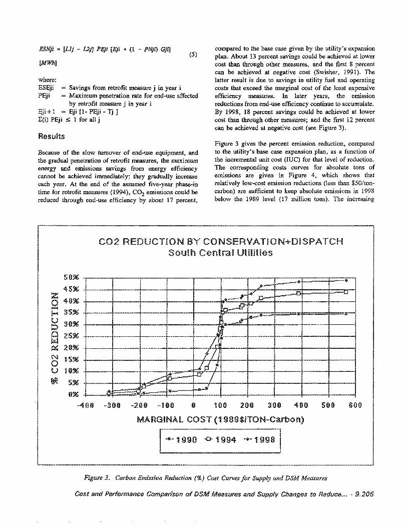
Because of the slow turnover of end-use equipment, andthe gradual penetration of retrofit measures, the maximumenergy and emissions savings from energy efficiencycannot be achieved immediately; they gradually increaseeach year. At the end of the assumed five-year phase-intime for retrofit measures (1994), CO2 emissions could bereduced through end-use efficiency by about 17 percent,

ESNji = [Llj - L2J] PEji [Eji ... (1 - PNjI) Gji]

[MWh]

(5)compared to the base case given by the utility's expansionplan. About 13 percent savings could be achieved at lowercost than through other measures, and the first 8 percentcan be achieved at negative cost (Swisher, 1991). Thelatter result is due to savings in utility fuel and operatingcosts that exceed the marginal cost of the least expensiveefficiency measures. In later years, the emissionreductions from end-use efficiency continue to accumulate.By 1998, 18 percent savings could be achieved at lowercost than through other measures; and the first 12 percentcan be achieved at negative cost (see Figure 3).

Figure 3 gives the percent emission reduction, comparedto the utility's base case expansion plan, as a function ofthe incremental unit cost (IUe) for that level of reduction.The corresponding costs curves for absolute tons ofemissions are given in Figure 4, which shows thatrelatively low-eost emission reductions (less than $50/ton­carbon) are sufficient to keep absolute emissions in 1998below the 1989 level minion tons). The increasing

2R U TI B R TIouth Central Utilities

+01 H

.... 4),,?.........--..

......---r .........0-- n. ----l'..J~

I_~ t..ru-- em-

11• ..-r!''"''11,..,..11

III

.."

l_Lid!

~~.......- -0'/0-----"'

-...A~ e_lfl

00 -200 -100 o 100 200 300 400 500 600

MARGINAL COST (1 9a9S/TON-Carbon)

Figure 3& Carbon Emission Reduction (%) Cost Curves for Supply and DSM Measures

Cost and Performance (.;omL~a!'J'S(Jln of DSM Measures and ~"IBnnAry GhaAr;gE~S to Reduce~ .. ~ - 9,,205

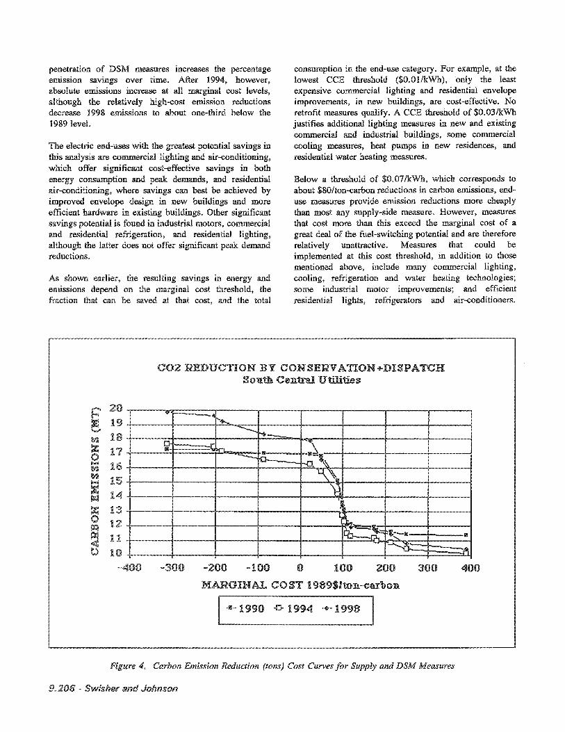
penetration of DSM measures increases the percentageemission savings over time.. After 1994, however,absolute emissions increase at all marginal cost levels,although the relatively high-cost emission reductionsdecrease 1998 emissions to about one-third below the1989 leveL

The electric end-uses with the greatest potential savings inthis analysis are commercial lighting and air-conditioning,which offer significant cost-effective savings in bothenergy consumption and peak demands, and residentialair-conditioning, where savings can best be achieved byimproved envelope design in new buildings and moreefficient hardware in existing buildings. Other significantsavings potential is found in industrial motors, commercialand residential refrigeration, and residential lighting,although the latter does not offer significant peak demandreductions"

As shown the savings in energy andemissions on the cost thefraction that can be saved at that cost, and the total

consumption in the end-use category.. For example, at thelowest CCE threshold ($O.Ol/kWh), ·only the leastexpensive commercial lighting and residential envelopeimprovements, in new buildings, are cost-effective. Noretrofit measures qualify. A CCE threshold of $O.03/kWhjustifies additional lighting measures in new and existingcommercial and industrial buildings, some commercialcooling measures, heat pumps in new residences, andresidential water heating measures..

Below a threshold of $Oo07IkWh, which corresponds toabout $80/ton-carbon reductions in carbon emissions, end­use measures provide emission reductions more cheaplythan most any supply-side measure.. However, measuresthat cost more than this exceed the marginal cost of agreat deal of the fuel-switching potential and are thereforerelatively unattractive.. Measures that could beimplemented at this cost threshold, in addition to thosementioned. above, include many commercial lighting,cooling, refrigeration and water heating technologies;some industrial motor and efficientresidential lights, refrigerators and air-conditionerso

19

~ 18

= 170~

~

~~

~ 14~

~0

=~ 11t) 10

CONSERVATION+DISPATCH'lIU"JlI"'%.'1BR111'l111"lIl'8>.. Central

-100 0 100 200

CO ST 1989$/1Dn-cu'bon

300 400

4$ Carbon Emission Reduction (tons) Cost Curves for Supply and DSM Measures

9~206 - ~MflSI'18r and Johnson

Measures analyzed here that are not cost-effective at thislevel include heat pumps and shell improvements inexisting residential buildings, and some industrial motorimprovements and commercial lighting retrofits ..

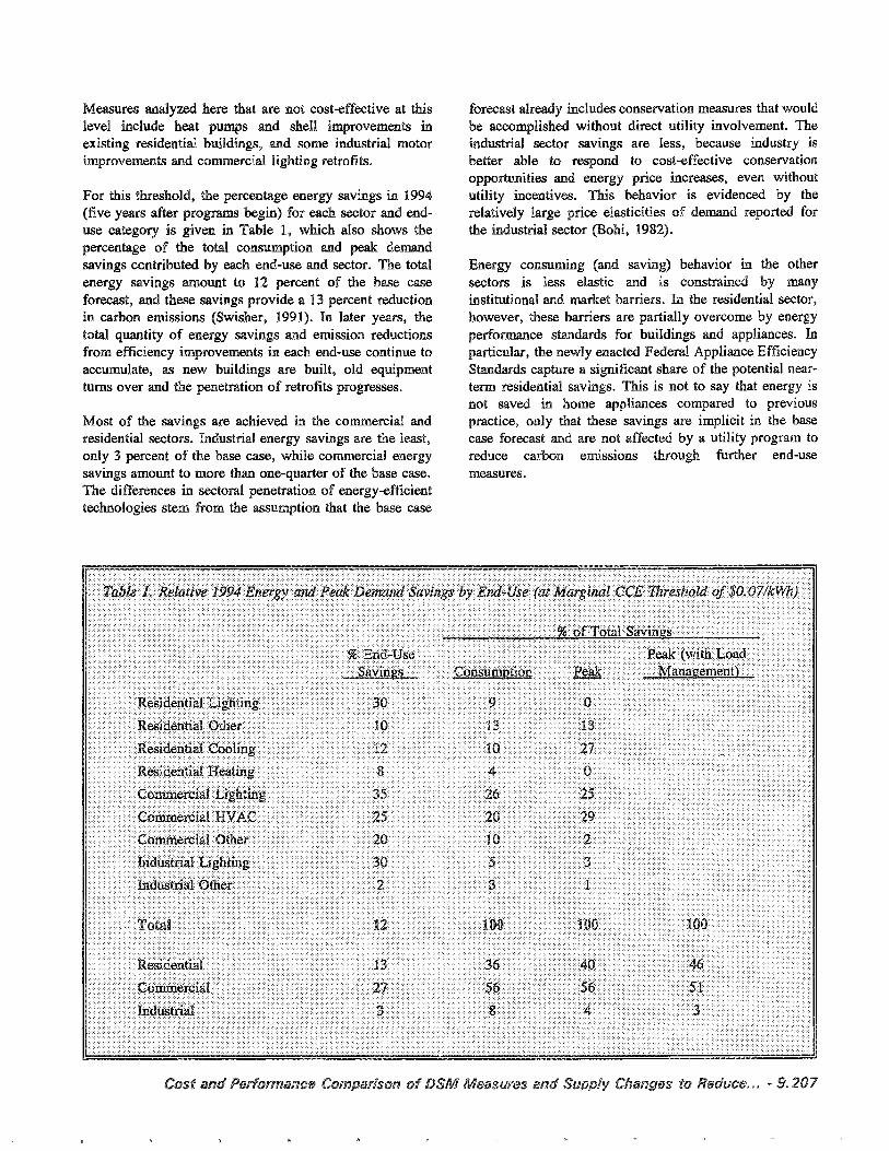
For this threshold, the percentage energy savings in 1994(five years after programs begin) for each sector and end­use category is given in Table 1, which also shows thepercentage of the total consumption and peak demandsavings contributed by each end-use and sector. The totalenergy savings amount to 12 percent of the base caseforecast, and these savings provide a 13 percent reductionin carbon emissions (Swisher, 1991). In later years, thetotal quantity of energy savings and emission reductionsfrom efficiency improvements in each end-use continue toaccumulate, as new buildings are built, old equipmentturns over and the penetration of retrofits progresses..

Most of the savings are achieved in the commercial andresidential sectors. Industrial energy savings are the least,only 3 percent of the base case, while commercial energysavings amount to more than one-quarter of the base case..The differences in sectoral penetration of energy-efficienttechnologies stem from the assumption that the base case

forecast already includes conservation measures that wouldbe accomplished without direct utility involvement. Theindustrial sector savings are less, because industry isbetter able to respond to cost-effective conservationopportunities and energy price increases, even withoututility incentives.. This behavior is evidenced by therelatively large price elasticities of demand reported forthe industrial sector (Born, 1982).

Energy consuming (and saving) behavior in the othersectors is less elastic and is constrained by manyinstitutional and market barriers. In the residential sector,however, these barriers are partially overcome by energyperformance standards for buildings and appliances. Inparticular, the newly enacted Federal Appliance EfficiencyStandards capture a significant share of the potential near­term residential savings.. This is not to say that energy isnot saved in home appliances compared to previouspractice, only that these savings are implicit in the basecase forecast and are not affected by a utility program toreduce carbon emissions through further end-usemeasures~

and Performance {,;oml.)al'J,so~nof Measures and C;h~an~'1es to Reduc8u$ - 207

Commercial energy efficiency is less affected by Federalstandards, particularly in the important lighting category..There are many mandatory and voluntary standardsdealing with the safety and performance of energy-usingequipment, but standards governing energy consumptionare weaker in most areas.. Furthermore, the large fractionof commercial space that is built on speculation andoccupied by tenants creates a situation where there arefew incentives to invest in energy-efficient buildings andequipment, no matter how cost-effective.. Because of therelative lack of either market or mandatory incentives forend-use efficiency measures, the untapped potentialappears largest in the commercial sector..

Commercial end-use technologies also provide the major­ity of peak demand reductions.. Because commercial light­ing and cooling contribute directly to summer peak loads,efficiency measures in these end-uses are especiallyeffective at reducing peak demand.. Residential coolingalso presents considerable potential for peak: loadreduction.. Further peak load reductions can be achievedthrough load management programs such as commercialthermal energy storage and direct load control of resi­dential air-conditioners.. These programs are not intendedto reduce carbon emissions directly, because they do notnec~ess:anjlV a4ecrlease~ and may increase total COllsumptlO][L

In these load programs do result inmodest reductions in emissions, due to the use of moreefficient in place of the lessefficient peak demand hours .. Althoughessentially neutral in terms of total emissions, the........... 11-.. _ ..................... effect of load programs is that

the use of variable-costae.laVltn~ the need for new plants and

load reducesthe entire program of emission

thrl()Uj]~.b DSM more cost-effective~

Supply-Side Options

""'A"UV".l~U most of the feasible """?''t"'Il''1~::Ilnt'''~1

achieved at an average cost of less thanthe most efficient is to ImlPleltneJltthe measures with the lowest cost At a marginalcost of about the can to significantlyreduce emISSions changing their order tobum more natural gas and less coal in their existing

The net cost of this measure varies with changes inheat rate efficiency) and variable operating costs,but the difference is the higher fuel cost for naturalgas~ most of the feasible savings from fuel-SWlltch.1n~ have a cost of $90 to $120 per ton-

I=SVVlstBer_ 1991).. Together with the less expensive

9.. 208 - SlIiflsJ)er and Johnson

efficiency measures, which provide the first 8 percentsavings at negative cost, fuel-switching makes it possibleto reduce emissions after five years by 35 percent at amarginal cost of $l00/ton, or 40 percent at $200/ton (SeeFigure 3)$

Beyond $200/ton-earbon incremental cost, additional emis­sion reductions can be achieved through further end-useefficiency measures.. Indeed, the total potential may begreater than shown here because such expensive measuresare not widely reported when they are not considered. cost­effective.. However, another relatively high-cost optionwould be to replace some existing and planned fossil fuelcapacity with non-eombustion resources, either solar ornuclear, or perhaps with fossil fuel plants fitted with C~emission control..

The base case expansion plan includes two nuclear stationsalready on-line and one under construction 0 Of course,because of the low variable costs and negligible carbonemissions of nuclear power, these plants are dispatched asbase load and operate as much as possible in all emissionreduction scenarios~ Some regions have significant hydro,geothermal, wind and solar resources that can yet beexploited.. The most promising renewable resources in thesouth-eentral appear to be solar in West Texas andperhaps wind in Oklahoma$ We considered two non­combustion options, nuclear power and line-focus solarthermal power in West Texas .. Nuclear power does notappear to have significant near-tenn potential for reducingCO2 emissions 0 Assuming a minimum construction lead

for a 1300 MW plant, of six years from the com­pletion of the plant already under construction, noadditional nuclear capacity could be operational before1999, too late to significantly figure in our results$

The solar thermal plants have a shorter lead time, but itwould take some time before the industry's building

could far surpass the current level of about80 MW per year.. Assuming a maximum construction ratein Texas of 160 MW per year, solar would not likelymake a significant impact on emissions until at least 1997..Cost and performance data (corrected for climate) weretaken from California Energy Commission projections forline-focus plants built for utility ownership, at larger scalethan the present plants and with no on-site gas-firedbackup (CEC, 1989)&

The existing expansion has two large coal-fired plantsdue to begin operation in 1997 ~ Either the aggressive solaror nuclear strategy would obviate the need for theseplants.. Indeed, neither supply strategy can save much inemissions, compared to the base case expansion plan, untilthe time these plants would be replaced.. Until then, thenon-fossil plants would replace gas-fired plants, resulting

in smaller emission savings.. In 1996, the solar plants canreduce emissions about 2 percent, at an incrementalcost of $1751ton, more expensive than most othermeasures.. By replacing the coal-fired plants, solar canreduce emissions by 7 percent in 1998, or nuclear couldprovide 11 percent reduction in the year 2000.. Eithertechnology, implemented by itself, would have anincremental cost of about $90/ton compared to the basecase, roughly equivalent to the cost of fuel-switching ..

Without the option of reducing emissions through inexpen­sive DSM, replacement of new coal-fired capacity withsolar or nuclear capacity would be competitive with thefuel-switching option, especially if gas prices wereexpected to increase more than assumed here.. However,these technologies will not represent least-costopportunities until the less expensive DSM measuresdescribed above have already been implemented. This isan example of how the supply-side effect of DSMmeasures can change the utility's incremental costs andemissions~ in a way that makes additional emission.reduction measures appear more expensive.

Extension to Other Regions

The results presented above apply to utilities in the south­central region of the U.S&, but one might expect similargeneral trends in other regions as welL The fonow~g

comparison of the regional variations in the results IS

based on a simplified analysis of the supply-side param­eters using MIDAS. Assuming that energy end-use effi­ciency improvements have the same costs and percentageenergy savings, these supply-side variations determine theregional differences in the emission reduction potential asa function of incremental cost" Of course, differences inclimate, building practices and costs, and existing end-usetechnology win create regional variations in the perform­ance of DSM measures as welL However, in the energyefficiency "supply curve" analysis performed to date inseveral regions, the total percentage energy savings for agiven end-use at a given cost level do not seem to varygreatly (Geller, et aL 1987; Miller, et at 1989) .. Rather,supply-side differences, especially the generating capacityand fuel mix, can be expected to drive most of theregional variations ..

The regional results are shown in 5, in the form ofincremental cost curves, for percentage carbon emissionreductions both DSM and supply-side measures& Thecurve for the south-central is the 1994 curve from

3" The results suggest si ificant differences acrossthe Because of the assumption of equal DSM per­formance across the regions, the percentage savings forthe DSM options are similar for each region.

The effect of is less for all the other1."'~Ji.V.8UI.0I9 compared to the south-central region. This resultreflects this region's relatively large amount of gas-fired

which allows for a large fraction of the load metcoal....fired plants to be shifted to gas-fired plants. The

west and northeast regions, which have relatively lessemissions before fuel-switching, can still achieve signifi­cant reductions because of their gas-fired capacity. Theother regions have both higher base-case emissions andless emission reduction potential because of less gas-firedcapacity, especially the east-central region, which is sodominated by coal....fired supply capacity that there is littlepotential for fuel switching, both in percentage terms andabsolute quantities. Only in the West do renewablesources contribute significantly by 2000, but their impactis diluted by the load....growth reductions available thoughend-use efficiency, as discussed above. Note that the east­central region produces greater absolute emissionreductions than the south-central region, and the west andnortheast regions produce less" These results simplyreflect the of the base case plan, which is

cost-effective of the conservation measuresto eliminate the need for the coal-fired

Dlannt~ for 1997& neither the solar nor thewould the new coal-fired plants, at

the As a the incremental emissionreduction from these would be about 40 per-cent as much as suggested above aremented This result reduces the savings for solar to2&5 1998) and for nuclear to 4&5 percent2000), and it increases the incremental cost from $90 to

3 shows these emission savingsfrom solar as a small increment at around $230/ton....carbon" Emission frOID nuclear would not appearuntil after 1998..

The other class of emission reduction tec:.hn!O!Ct2U~S

involves emissions from the powergases. This is the most common method of mJ1tH!~ltl{]l2

emissions" from combustion product gasesnew that would not

reduce other emissions. enussionsare about 100 times in volume than S02 emissionsfrom a coal and is less reactivethan In the mass of in the stack gas isthree times that of the coal fuel! the feasibility of

removal and considering the huge materialis very speculative at present One

recent estimate the cost of direct CO2 control, if itcould be done, at over $500/ton-carbon and

1989)*

Cost and Performance Co~rnlJ,ar/~~on of DSM Measures and ~~"",--j',,# {;'t18J1fJ6'S to Reduce".,,, - 9,,209

REDUCTION BY CONSERVATION+DISPATCH---J_--,............... Va:riations - 1994

A. ~

p--~v

~f.J

L,...-...---iII IJ!iII

m""'-

fi--!'''m7 A J\

'~~-..~

'C ...A -..l -~

.....,~il A~

-~+

tr _.A~~.

-I;Z-- _n -'--..-0

7) ~~

~

.--~"l1IlI" :JIIIIIIIIIIl'l :I;f

......-~ '1l~:""""""-

J.~ ¥

---J:J~l.J

-200 -100 600500o 100 300 400

.rGIoolllll.1lIl§O-'~ COST (1989$/TOH-Carbon)

45~

40~

35~

30~

25~

20~

15~

1096

5~

O~

-400

Cent .... Southeast

5~ Carbon Emission Cost Six Geographic KeJUOI1,s

Another feedback results from the changes inrevenues due to end-use measures such as energy end-use

The costs of the end-use measures will tend toincrease and lead to a feedback similar to thatdescribed above.. even if the cost to the utility

The cost of reduction measures does notconsider the feedback of in

caused increased costs and lost saleso In general,cost fuel for

eX~lm.i)le~ win raise costs and in decreaseddemand and additional reductions in emissionso theaverage cost of the reductions are reduced somewhatthis effect This benefit comes at the expense of consumer

lost from the increase..

for the east-centralin the west and northeast

Effects of Price Feedback

and lower of a DSM program is zero, the may have toto compensate for revenues lost due to the

energy This result occurs when price is greaterthan short-run cost (as in this case study),because for every kWh the utility saves thema.r2:1nal cost and loses the price (assuming zero cost ofsaved energY)e The price increase leads to decreasedoelJnaDd. especially for non-participants (Hobbs, 1990).. Asthe cost of the end-use measures increases, this effect isenhancecL

How great is the price feedback effect from the end-useefficiency measures considered in this analysis? To answerthis question, let us again concentrate on" the $Oe07/kWhmarginal CCE threshold, where most of the attractivemeasures have been implemented" The average cost to the

(net of utility cost savings) at this level is almostzero.. the price feedback effect would only resultfrom increases due to lost revenues, not fromincreased costs ..

9,,210 - Swisher and Johnson

gies is still relatively uncertain, and new technologicaldevelopments might make additional end-use efficiencymeasures attractive beyond those analyzed here.. Althoughend-use efficiency opportunities may become saturatedover time, exploiting these opportunities in the near-termcan control emissions at reasonable costs while advancedsupply technologies are being developed ..

California Commission 19890 Technology Char-acterizations for 10"'1""$'"1,,"',n7 Report 90.. CEC Staff

Sacramento..

L.. 19890 The Administrative CostsConservation Oak National .L.ai)0f41tOl~V

Oak Ridge, TN, ORNL/CON-294 ..

ckno ledgement

Parts of this work were the Electric PowerResearch Institute (EPRI)o AU views expressed are thoseof the authors and do not necessarily reflect the positionsnor policies of EPRIo comments came from PhilHanser, Jan Borstein and an anonymous reviewero

References

Do 1982.. Price Elasticities ofDemand forEvaluating the Estimates, Electric Researchlnst:Itute~ Palo Calif.. , EPRI EA-26120

Chernick and Es CaverhiU 19890 The Valuation ofExternalities from Energy Production, and UsesPLC Boston..

As stated earlier, the utility is assumed to implement end­use programs by direct investment, recovering the coststhrough the rate base (as expenses) .. The details of howand from which customers the costs would be recoveredare not considered.. However, one possibility is that theutility selectively recovers some fraction of the costs fromthe beneficiaries of the investments, i..e. the rticipants inthe DSM program.. This approach reduces the fraction ofcosts that must be recovered from the non-participants,thus mitigating their price increase and the resultingdemand feedback" Also, improved end-use efficiencymakes an end-use less expensive at the margin for theparticipant, producing a positive price feedback ondemand" This rebound effect is limited because partici­pants normally have smaller price elasticities than non­participants (Henly, et at 1988). Also, most of thesavings are achieved in the residential and commercialsectors, which have relatively low price elasticities ofdemand.

onclusion

With low DSM investment costs, cost recovery,and the participants' rebound effect, there are manypressures 'the feedback effects of end-useefficiency investment and lost revenue.. At an average unitcost of zero, it is possible that the combination of thesepressures could for the revenue effect

the more feedback effect is thatcaused a average unit cost of the DSMmeasures" This feedback is similar to that causedother of cost such as to more~Yl,\~"f;;::n}'~ fuel or other measures °

/OP:'.".1 I"" "7 Con-

Efficient

Electric Power Research Institute 1989& The EPRIElectric Power Research

Calif.. , EPRI P-6211"

Electric Power Research Institute 1988. Technical Assess­ment Guide vol.. 20 Electric Power Research Institute, Palo

EPRI P-4463-SRo

H .. , et at 1987.. Acid Rain andservationo American Council for an

Washington.

et aL 1988.. MlDAS-Multiobjective Intl'-~orf"tpl1

Decision Analysis System User ManuaL Electric PowerResearch Palo Calif., EPRI P-5402-CCM.

J", et aL 1988"f\U~Op{lOn of More Efficient APPi1:anc:es"

." .... ""'."" ... A~ .. _ voL 9, pp 163-1700

The results in 4 and 5 thatsubstantial near-term reductions in carbon emis-

on the order of 35 or more for the casecould be achieved at a cost of less

" rrnl-l~aT'nnli1 ~ This that a carbon tax onthe order of would stimulate utilities to invest inmeasures to achieve reductions of this Altema-

if the of carbon emission or someother market-based were as as $100/ton,the same result would be achieved ..

more than half of the 35 emissionreduction achieved. at an incremental cost of $100/ton­carbon results from fuel and on the

the remainder is from end-use efficiencyJ"'U."H.U'J,~H this analysis does not extend far into

the it appears that non-fossil generating sourcessuch as nuclear and/or solar energy would be able to com-

for future load and maintain emissions atthe reduced level" Of course, the cost of these technolo-

and Performance (;oml.)lJr",so'n of DSM Measures and _0."........... ,.".8 (;'naJ7gE~S to Reduce"o" - 9,,211

Hobbs, B.F.. 1990. "The Most-Value Criterion: EconomicEvaluation of Utility Demand-Side Measures ConsideringCustomer Value," The Electricity Journal.

Hunn, B.. D. et at 1986. Technical Potentiallor ElectricalEnergy Conservation and Peak Load Reduction in TexasBuildings.. Public Utility Commission of Texas, Austin..

Meier, A., et a1.. 1983. Supplying Energy ThroughGreater Efficiency.. University of California Press,Berkeley..

12 - and Johnson

Miner, P.M., et a1. 1989.. The Potential for ElectricityConservation in New York State.. New York State EnergyResearch and Development Authority II

Northwest Power Planning Council 1986. Northwest Con­servation and Electric Power Plan 1986. NWPPC,Portland..

Swisher, J.N,. 1991 .. Prospects for International Trade inEnvironmental Services,,· An Analysis of InternationalCarbon Emission Offsets. PhD Thesis, StanfordUniversity, Civil Engineering Dept..