cost-benefit analysis of the effects of implementing sea...

Activity 2 – Defining Sea Traffic Management

Cost-Benefit Analysis of the Effects of Implementing Sea Traffic Management in

the Northern Parts of the EU

MONALISA 2.0 — COST-BENEFIT ANALYSIS OF IMPLEMENTING STM IN NORTHERN EU 1

Document Status Authors

Name Organisation

Peter Andersson Linköping University

Pernilla Ivehammar Linköping University

Review

Name Organisation

Approval

Name Organisation Signature Date

Björn Andreasson SMA 2015-12-22

Document History

Version Date Status Initials Description

1.0 2015-12-22 Appr. Final deliveravle for ML 2.0

TEN-T PROJECT NO: 2012-EU-21007-S

DISCLAIMER: THIS INFORMATION REFLECTS THE VIEW OF THE AUTHOR(S) AND THE EUROPEAN COMMISSION IS NOT LIABLE FOR ANY USE THAT MAY BE MADE OF THE INFORMATION CONTAINED THEREIN.


Table of contents 1. Introduction ................................................................................................................. 5

1.1 Sea Traffic Management ......................................................................................... 5

1.2 Aim of the study ...................................................................................................... 6

1.3 Outline of the study ................................................................................................. 6

2. Methodology ............................................................................................................... 8

2.1 Cost-benefit analysis ............................................................................................... 8

2.2 Data ........................................................................................................................ 8

3. Volume of traffic in the northern parts of the EU ................................................... 10

3.1 Method for measuring the volume of traffic ............................................................ 10

3.2 Ship types ............................................................................................................. 12

3.3 Volume of traffic in the selected areas ................................................................... 13

4. Volume of anchored ships awaiting berth in the EU part of the Baltic Sea .......... 15

4.1 Method for measuring the volume of traffic ............................................................ 15

4.2 Methodology for estimating the total volume of anchored ships ............................. 16

4.3 Volume of anchored ships in the selected area ..................................................... 17

5. Estimating costs of sea transportation ................................................................... 19

5.1 Fuel costs .............................................................................................................. 19

5.2 Emission costs ...................................................................................................... 20

5.3 Manning costs ....................................................................................................... 22

5.4 Capital costs ......................................................................................................... 24

6. Benefits of route optimisation ................................................................................. 25

6.1 Total costs for sea traffic in the northern part of the EU ......................................... 25

6.2 The potential for route optimization ....................................................................... 28

6.3 Benefits of shorter routes ...................................................................................... 29

7. Benefits of adjusted arrival times ............................................................................ 31

7.1 Methodology for calculating the benefits ............................................................... 31

7.2 Benefits of adjusting arrival times .......................................................................... 32

8. Costs for the project ................................................................................................. 35

8.1 Costs related to the ships ...................................................................................... 35


8.2 Costs related to the ports ...................................................................................... 36

8.3 Costs for governance ............................................................................................ 37

8.4 Summary of estimated costs ................................................................................. 37

9. Case study: The benefits of Port CDM in the Port of Gothenburg ........................ 39

10. Cost-benefit analysis of Sea Traffic Management ................................................ 41

10.1 Benefits and costs of route optimisation with constant safety .............................. 41

10.2 Benefits and costs for Port CDM with adjusted arrival times ................................ 43

10.3 Additional benefits from increased safety with STM............................................. 44

10.4 Summary of benefits and costs ........................................................................... 44

10.5 Results in an EU perspective .............................................................................. 46

10.6 Improved knowledge in MONALISA 2.0 .............................................................. 47

10.7 The need for further studies to validate the results .............................................. 47

REFERENCES ............................................................................................................... 48


1. Introduction Increased international trade together with the intention to reduce global emissions leads to increasing needs to make transportation at sea as efficient as possible. The availability of data from ships’ AIS-transmitters provides new opportunities to quantify traffic and better evaluate proposals aimed at making sea transportation more efficient.

1.1 Sea Traffic Management The MONALISA 2.0 project has developed the concept “Sea Traffic Management (STM)”, aimed at increasing safety, environmental and operational efficiency for maritime transportation. STM includes the four sub-concepts “Strategic voyage management (SVM)”, “Dynamic voyage management (DVM)”, “Flow management (FM)” and “Port collaborative decision making (Port CDM)” These four concepts are supported by a “System-Wide Information Management architecture (SeaSWIM)” concept that will support current and future systems used by the maritime industry by providing a distributed, flexible, and secure information management architecture for sharing information. (Lind et al, 2014, Smith, 2015). This study focuses on the sea transportation part of these four central concepts of STM, and possible savings in the port due to Port CDM.

SVM is the preliminary planning of the route before the voyage takes place. The main objective with the DVM is to iteratively adjust the original voyage plan in order to always run the ship in the most cost-efficient and safe way, using all possible in-data that can affect the voyage plan. Flow Management aims at optimising the total traffic situation in a given area with the help of updated information about the intended routes of ships in that area.

With shared information ships may take a more optimal route, mainly taking other ships’ movements into account as well as other factors such as weather, ice and traffic restrictions. The overall aim is to save fuel, travel time and capital costs as well as reducing the environmental impact of shipping, and increase safety.

Port CDM builds on the sharing and providing of information between different stakeholders related to the port for the purpose of providing situational awareness and instant sharing of changes related to the port call process, enabling each actor to make accurate plans. The sea transportation part of Port CDM requires updated information about berthing times, based on which ships could adjust their speed to arrive at the port just in time. Thereby, ships could sail at a more fuel-efficient speed without increasing the transit time of the cargo. Moreover, Port CDM may lead to better utilization of infrastructure and resources in ports.

Thus, an introduction of STM creates a potential for ships both to optimise routes, the possibility of achieving just in time arrival at ports, adjusting to a more fuel-efficient speed and enabling each actor in the port to make better plans and utilize available resources


more optimal. However, STM requires investments both ashore and in equipment on board participating ships as well as costs for operating the system.

1.2 Aim of the study A first study of the Baltic Sea Region was carried out as part of MONALISA 1, estimating potential benefits and costs of using shorter routes and adjusting arrival times at ports. The analysis was based on AIS-data and unit costs (Andersson, Ivehammar, 2014), and showed that the benefits of dynamic route planning widely outweigh the costs. The current report will present results from a second study, using AIS-data provided by the Swedish Maritime Administration (SMA) and publicly available AIS-data. An area comprising most of the northern EU waters is selected, longer time periods are studied, and updated and more comprehensive data and unit values are used in the valuation of effects. The previous study focused on dynamic route planning, whereas this second study includes the broader concept of Sea Traffic Management. The aim of the present study is to conduct a cost-benefit analysis in order to estimate the benefits and costs for society as a whole of implementing STM in the northern part of EU.

1.3 Outline of the study The initial part of the study measures the potential savings from route optimisation. The volume of sea traffic for the northern parts of the EU, comprised of two major areas in the North Sea and in the Baltic Sea, is first calculated, based on complete AIS-data for three selected days. Then, the total costs of the traffic is calculated by using the updated unit values and formulas for fuel, manning and capital costs as well as costs for emissions. This provides a basis for the estimation of the total potential for savings by achieving shorter routes after the introduction of STM.

The second part of the study focuses on adjusted arrival times as part of Port CDM. Today contracts often stipulate that ships should arrive as soon as possible, whether or not a berth is available, i.e. a “hurry up and wait”-principle (Alvarez et al., 2010). The ship may have to anchor before entering a port because the berth may be occupied, the cargo may not be ready, adjustment of berth time to tides or channel operations, etc. During the analysis, a lack of information has been identified regarding the extent to which ships of different types and categories anchor, awaiting to enter the port and do not lie at anchor for other reasons, and for how long time they lie at anchor. Hence, AIS-data from anchored ships outside ports in the EU countries of the Baltic Sea are gathered through public AIS-data. Data is collected for the Baltic Sea during twenty occasions with follow-up during April and May to achieve the extent of anchoring awaiting berths in the area. Based on this data, estimates are made about the potential savings by arriving just in time, depending on for how long before original ETA (estimated time of arrival) a ship’s speed can be adjusted, and how much fuel this will save.


The third part of the study focusses on the potential savings in ports by implementing Port CDM, examined in a separate report by Merkel (2015). A summary of that report concerning the gains of higher resource utilization and shorter turn-around times is presented in this report. The benefits from savings identified in the three parts of the study are then compared with the costs for the system. There will be costs for developing technology and investments in equipment as well as for training and for running the system. Governance of such a system may also be necessary.

The possible gains for society as a whole are analysed, by estimating the benefits and costs of implementing STM. By society, all parties that in one way or another are affected by sea transportation are included, i.e. the buyers and sellers of the services but also society as a whole, e.g. if there are positive or negative effects on the environment. The potential effects on freight flows ashore are not included in the calculations.

As participation in STM is not intended to be mandatory, costs (and benefits) will depend on the propensity to join the system. In this report it will be assumed that all involved ships and ports will participate in the system. Only effects on traffic with cargo ships and tankers will be accounted for. All figures are stated in euro, the price level as of June 2015.1

1 The exchange rate for June 15: 9.23 SEK/euro (The Riksbank, 2015) and 1.12 USD/euro are used, when transferring values originally provided in SEK or USD. Values are recalculated to the price level of June 15, 2015 with consumer price index (www.scb.se).


2. Methodology 2.1 Cost-benefit analysis A cost-benefit analysis (CBA) is based on welfare theory (Boardman et al., 2011). This theory is about achieving as much benefit as possible with the scarce resources available. The concern is the well-being of society as a whole, including all individuals, all firms and the public sector. The aim of a cost-benefit analysis is to provide a basis for decisions in order to maximise the total welfare in society. Since resources are scarce, only changes where the benefits exceed the costs should be implemented. All parties that are affected in one way or another by the studied change (often called a project), should be included in the CBA. The valuation should if possible be based on the involved actors’ own preferences. A central part of CBA is opportunity cost, i.e. the cost of resources used in a project is equal to the value of their best alternative usage.

The methodology in a cost-benefit analysis is that all effects of a proposed project are first identified. For example, a new road might save travel time and improve safety, but at the same time uses material and labour and might make intrusion in some recreational area. In a second step, these identified effects of the project are, if possible, quantified. How much travel time would the new road save, how much material would be used to build the road and how would the road encroach on the environmental area etc. The third step is to try to estimate the value of all effects in monetary terms by for example using values per unit for travel time savings. Some identified effects may not be measurable in such a way, but should still be part of the cost-benefit analysis. Effects without an estimated value should be described in words. Some effects will occur only once while other effects may occur several times over the project’s lifetime. The effects which are evaluated in monetary terms are therefore discounted to be comparable. Finally, the effects are summed up to find out if the benefits exceed the costs. Some effects as well as values may be uncertain, and a sensitivity analysis, to evaluate the robustness of the conclusions, should be carried out.

2.2 Data In this study, the traffic is quantified using Automatic Identification System (AIS) data from ships in the Baltic Sea and the North Sea. The technology allows measuring the total sea traffic in the selected areas. It is mandatory since 2007 for commercial ships above 300 gross tonnage (GT) to have an AIS transmitter that continuously sends a signal with information about the ship (e.g. position, speed, course, destination and data about the ship) (EU Directive 2013/52/EU). Depending on the ship’s speed, a signal is registered with different frequencies, and a single ship’s position and other data can be registered and result in over 1,000 observations in one day. The designated organisations of the HELCOM member states collect data from all ships with AIS transmitters in the Baltic Sea Region. This data has been made available via SMA. Ships’ AIS data is also visible in real time on the publicly available internet site MarineTraffic. AIS data from tailor-made


files, produced by SMA, are used to calculate the volume of sea traffic in the northern parts of the EU, and real time AIS information on the internet site MarineTraffic is used to measure the extent of anchored ships in the Baltic Sea.

Ships’ fuel consumption, which is an important input to compute costs, is calculated based on the ships’ AIS-data. The fuel consumption of each individual ship is estimated based on each ships speed, beam, draught and length. For estimating emissions, established relationships between fuel consumption and emissions are used. The unit values for emissions used in transport infrastructure planning in Sweden as well as values from different European studies are used for the evaluation. Other costs for operating ships are taken from different reports, contacts with Swedish ship owners and the Swedish Maritime Administration. The costs for the project have been estimated by different participants in the MONALISA project.


3. Volume of traffic in the northern parts of the EU

3.1 Method for measuring the volume of traffic Three days are selected for which complete AIS data is delivered from the Swedish Maritime Administration (SMA) for one area in the Baltic Sea and one area in the North Sea, in order to estimate the total volume of sea traffic that could be affected by STM. The selected area in the Baltic Sea is chosen to represent the sea traffic in waters related to the EU-countries. Sea traffic in the Gulf of Finland is excluded, since it includes most traffic to Russian ports. As it is only possible to select squared formed regions for analysis, it was not possible to include the Bay of Bothnia without also including all traffic along the Norwegian west coast. The selected area in the North Sea consists of data which are gathered by Danish authorities and shared with SMA. No other data for the rest of the North Sea or the Mediterranean Sea was available by SMA at the moment of conducting the study. Hence, the area studied will be referred to as the northern parts of the EU, comprising the studied areas in the Baltic Sea and the North Sea. The shaded areas in figure 3.1 and 3.2 show analysed areas. Figure 3.1 The studied area in the Baltic Sea

Source: The Swedish Maritime Administration


Figure 3.2 The studied area in the North Sea

Source: The Swedish Maritime Administration

The selected days are September 1, 2014; February 4, 2015 and April 10, 2015. They are chosen to be normal days. There were no limitations from ice in the selected areas. The summer period is avoided since commercial traffic may be reduced, and there are also many cruise ships in the region. On the days in question, there were no strong winds or waves which could have caused the ships in the selected areas to sail slower or await better weather conditions.

Moreover, the study is confined to ships registered as ‘cargo’ (including general cargo, bulk, ro-ro, automobile carriers, and container) or ‘tanker’ with a 300 GT or above. Ferries are excluded as it is assumed they normally already have optimised their routes and that there are limited scope for them to shorten distances with the introduction of STM. Tugboats, pilot ships, and ships categorized as ‘other’ are also disregarded. A lower limit of 60 meters and 300 GT is used for the AIS data to exclude ships that are considered not to be relevant for the study. Based on these selection criteria, SMA delivered six files, one for each of the chosen days and areas, with all data from the AIS transmitters from cargo ships and tankers.

There were 75 % as many ship voyages in the selected area of the North Sea as compared to the selected area of the Baltic Sea. However, the files for the Baltic Sea


contained almost one million observations and the ones for the North Sea just over a hundred thousand. The large difference in the number of observations can be explained by the fact that, according to SMA, AIS signals are registered less frequently in the North Sea. In addition, when ships move slowly, change speed and course, ships send signals more frequently than when heading straight forward. In the selected area in the Baltic Sea ships enter or leave ports and narrow waters, unlike in the North Sea, where ships more often sail on a straight line and at a more even speed.

To calculate the costs, the sailed distance for each ship must be measured. AIS data only contains the actual speed at the moment of observation. Thus, for each ship, the average speed is calculated from all observations during the whole time of the 24 hour period that the ship was underway, and subsequently multiplied with the total time sailed during the day. The distance is then converted into meters. Observations when the ships’ speed was below one knot are excluded, as this may reflect manoeuvring in a port or moving while lying along a berth or at anchor. A few ships have more than one time period during the 24 hour period when they were moving, i.e. approaching a port in the morning and leaving in the evening. Such occurrences are analysed separately, as if there had been two different ships. The fact that ships send AIS signals less frequently in the North Sea may make the calculation of average speed and sailed distance somewhat less reliable than for the Baltic Sea. However, at sea, ships seldom change speed so the calculated average is considered accurate. The time underway for the ships may however be slightly underestimated in the North Sea, if the ship entered or exited the area before or after the first or last observation. This inaccuracy has been estimated to be only a few minutes; hence it will have an insignificant impact on the final results.

Information about each individual ship’s GT as well as the type of cargo ship, i.e. general cargo, container, roro/automobile carrier or bulk is gathered at the website of MarineTraffic (2015), since this information is not available from AIS data. This information is needed since some of the cost data is related to GT and type of ship.

3.2 Ship types In a report by the Swedish Environmental Protection Agency (SEPA, 2010) ships sailing in Swedish waters are categorised into different types. The ship types are taken from the Finnish system for calculations called LIPASTO2. This is a system used to calculate emissions representative for maritime traffic in Finnish waters and its surroundings. SEPA (2010) has made a selection from the ship types in LIPASTO aimed to represent maritime traffic in Swedish surrounding waters. Each such category represents an average of ships of different age, type, condition, load etc. within the category. The ships are sorted into categories based on SEPA (2010), since some of the cost data is based on these categories.

2 http://lipasto.vtt.fi/indexe.htm


http://lipasto.vtt.fi/indexe.htm

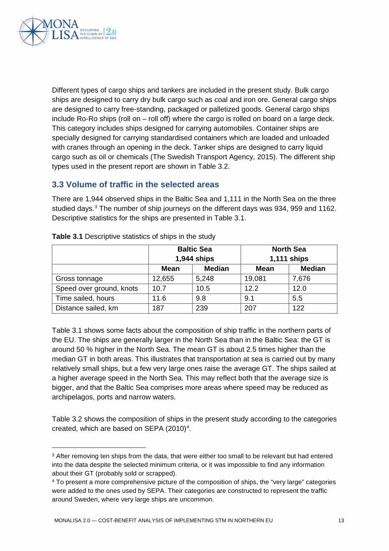
Different types of cargo ships and tankers are included in the present study. Bulk cargo ships are designed to carry dry bulk cargo such as coal and iron ore. General cargo ships are designed to carry free-standing, packaged or palletized goods. General cargo ships include Ro-Ro ships (roll on – roll off) where the cargo is rolled on board on a large deck. This category includes ships designed for carrying automobiles. Container ships are specially designed for carrying standardised containers which are loaded and unloaded with cranes through an opening in the deck. Tanker ships are designed to carry liquid cargo such as oil or chemicals (The Swedish Transport Agency, 2015). The different ship types used in the present report are shown in Table 3.2.

3.3 Volume of traffic in the selected areas There are 1,944 observed ships in the Baltic Sea and 1,111 in the North Sea on the three studied days.3 The number of ship journeys on the different days was 934, 959 and 1162. Descriptive statistics for the ships are presented in Table 3.1.

Table 3.1 Descriptive statistics of ships in the study

Baltic Sea 1,944 ships

North Sea 1,111 ships

Mean Median Mean Median Gross tonnage 12,655 5,248 19,081 7,676 Speed over ground, knots 10.7 10.5 12.2 12.0 Time sailed, hours 11.6 9.8 9.1 5.5 Distance sailed, km 187 239 207 122

Table 3.1 shows some facts about the composition of ship traffic in the northern parts of the EU. The ships are generally larger in the North Sea than in the Baltic Sea: the GT is around 50 % higher in the North Sea. The mean GT is about 2.5 times higher than the median GT in both areas. This illustrates that transportation at sea is carried out by many relatively small ships, but a few very large ones raise the average GT. The ships sailed at a higher average speed in the North Sea. This may reflect both that the average size is bigger, and that the Baltic Sea comprises more areas where speed may be reduced as archipelagos, ports and narrow waters.

Table 3.2 shows the composition of ships in the present study according to the categories created, which are based on SEPA (2010)4.

3 After removing ten ships from the data, that were either too small to be relevant but had entered into the data despite the selected minimum criteria, or it was impossible to find any information about their GT (probably sold or scrapped). 4 To present a more comprehensive picture of the composition of ships, the “very large” categories were added to the ones used by SEPA. Their categories are constructed to represent the traffic around Sweden, where very large ships are uncommon.


Table 3.2 Number of ships of each type in the present study

The distribution between cargo ships and tankers is almost the same in both areas: about 75 percent are cargo ships and 25 percent tankers. Again, it is visible that most traffic is with relatively small ships. In the Baltic Sea, 53 percent of the ships are below 6,000 GT and in the North Sea 44 percent is below 6,000 GT. There are fewer smaller ships in the North Sea and a larger share of large ships in all categories except large tankers in this sample. The second most common type of ship after small cargo ones are large bulk and large tankers. They also contribute to a large part of the costs, which will be showed in Chapter 5.

Ship type GT Baltic Sea North Sea cargo Cargo small 300-5,999 843 43.3 % 393 35.3 %

Bulk medium 6,000-13,999 98 5.0 % 68 6.1 % Bulk large 14,000- 167 9.1 % 143 12.8 % RoRo (incl automobile) 6,000- 113 5.8 % 68 6.1 % Container medium 6,000-13,999 129 6.6 % 66 5.9 % Container large 14,000-69,999 92 4.7 % 70 6.3 % Container very large 70,000- 7 0.4 % 34 3.0 %

tanker Tanker small 300-5,999 181 9.3 % 98 8.8 % Tanker medium 6,000-13,999 64 3.3 % 45 4.1 % Tanker large 14,000-69,999 242 12.4 % 114 10.3 % Tanker very large 70,000- 8 0.4 % 13 1.2 %

Total 1,944 1,111


4. Volume of anchored ships awaiting berth in the EU part of the Baltic Sea

4.1 Method for measuring the volume of traffic The frequency of ships that have to wait outside the port before berthing is studied. In the AIS data supplied by the Swedish Maritime Administration (SMA), it is not easy to separate ships that are not moving because they lie in a port from lying at anchor. Specific areas have to be defined, but as ships may anchor at many different locations, it is not easy to identify all such areas. The study to be presented finds that during the 20 studied occasions, ships had anchored outside 86 different EU-ports in the studied area. Moreover, it is difficult to identify which anchored ships are relevant to the present study, i.e. really waiting for berth or port to be ready in a port and not for other reasons. To find out which ships were anchored waiting for berth, and information about the ships, complementary data for all ships entering all ports in the area for the time period must also be analysed. Therefore data of ships lying at anchor in the Baltic Sea are collected from the Web site MarineTraffic to be able to study anchoring outside all EU-ports in the Baltic Sea in an effective way.

We make observations of anchored ships displayed at the Web site MarineTraffic (2015) on twenty occasions in April and May 2015. All ships anchored at a specific moment are observed and those ships which are anchored waiting to enter a port are registered and all other ships lying at anchor for other reasons are excluded. The registered ships are then followed up to find out for how long each one anchors before berthing and to verify that the ship actually enters the port of destination. The occasion of the primary observation are selected with approximately 48 hours interval. The time of observation is selected to cover both weekdays and weekends and observations are also made at different times to cover daytime and night time. Table 4.1 shows the weekday and time of day for the 20 moments observed. Table 4.1 Occasions when anchored ships were observed

Weekday Date and time of first observation Monday 27 April at 14.00 11 May at 22.00 25 May at 15.00 Tuesday 21 April at 07.00 5 May at 06.00 19 May at 10.00 Wednesday 13 May at 23.00 27 May at 03.00 Thursday 23 April at 14.00 30 April at 01.00 7 May at 21.00 21 May at 8.00 Friday 1 May at 21.00 15 May at 11.00 29 May at 09.00 Saturday 25 April at 13.00 9 May at 19.00 23 May at 18.00 Sunday 3 May at 16.00 17 May at 9.00

Ships can be anchored for many different reasons and the intention is to only include those ships which have to anchor outside a port while awaiting their berthing time. Thus those ships coming out from a port waiting for orders, ships anchored in order to take bunker (this is mainly present outside of Gothenburg and Skagen, where ships stop on


their way to or from the North Sea to take bunker from small tankers), ships anchored because of technical problems, and ships that unload at sea, are all excluded from the analysis. Hence, only ships that in fact did turn out to wait for berth are registered.

All ships lying at anchor in the area at the time of observation are registered, with data of how long they had already been lying at anchor, destination (port noted in the AIS data), ship type, length, beam, draught, average speed during the last journey and the GT of the ships. Twenty-four hours later, all ships are checked again to find out if they are still anchored, and if not, for how long after the first observation they had been at anchor. The ships are followed up until berthing in the port and on the next occasion of observation, the ships still waiting for berth from earlier occasions are not included in the new observation, to not double count any ships.

A possible problem is if some ships have their transponder turned off or if their self-reported status is incorrectly stated “for orders”. This could lead to missing some ships actually anchored awaiting berth.

4.2 Methodology for estimating the total volume of anchored ships The collected data is used to estimate the extent of anchored ships waiting for berth in ports in the EU-part of the Baltic Sea in a year. Thus, data is collected for Sweden, Denmark, Germany (the Baltic Sea part), Poland, Lithuania, Latvia, Estonia and Finland. From the number of ships lying at anchor at one moment on each of the twenty occasions, and the total time they were lying at anchor, the extent of ships lying at anchor in the area for a year is estimated. Making an observation at one moment during a 24-hour period gives only a 1/24 probability to register all ships anchored only for one hour within that period of time. To obtain the right number of ships anchored for one hour during a period of 24 hours, the observed number is multiplied by 24. For ships lying at anchor 2 hours, the chance of observing is 2/24, thus that number is multiplied by 24/2, for ships lying at anchor for three hours by 24/3 etc.

The estimation of number of ships in a period of 20 days is calculated as

∑ 24

ℎ𝑖𝑖𝑛𝑛𝑖𝑖=1 , 1 ≤ ℎ𝑖𝑖 ≤ 24 (4.1)

where n is the number of observed ships totally at the twenty occasions and h is the anchored time in hours. The estimation of number of ships in a year is calculated as ∑ 24

ℎ𝑖𝑖∗ 360

20𝑛𝑛𝑖𝑖=1 , 1 ≤ ℎ𝑖𝑖 ≤ 24 (4.2)


4.3 Volume of anchored ships in the selected area Table 4.2 shows the number of ships anchored by time anchored waiting for berth in ports in the EU-part of the Baltic Sea. Table 4.2 Number of anchored ships in the EU-part of the Baltic Sea, by anchored time

Hours anchored

Number of ships in total at the 20 occasions

Estimated number of ships in a period of 20 days

Estimated number of ships per year

1 2 48 864 2 6 72 1,296 3 5 40 720 4 9 54 972 5 2 9.6 172.8 6 5 20 360 7 6 20.6 370.3 8 4 12 216 9 3 8 144 10 8 19.2 345.6 11 8 17.5 314.2 12 7 14 252 13 5 9.2 166.2 14 9 15.4 277.7 15 5 8 144 16 7 10.5 189 17 6 8.5 152.5 18 4 5.3 96 19 13 16.4 295.6 20 7 8.4 151.2 21 5 5.7 102.9 22 10 10.9 196.4 23 10 10.4 187.8 ≥24 373 373 6,714 Total 519 817 14,700

Table 4.3 shows the anchored ships distribution by countries that the ports are located in.


Table 4.3 Number of anchored ships in the EU-part of the Baltic Sea, by country

Area Number of ships anchored in total at the 20 occasions

Estimated number of ships anchored in a period of 20 days

Estimated number of ships anchored per year

Denmark 48 57.7 1,039.3 Kiel Canal 13 70.8 1,273.9 Rest of Germany 48 75.0 1,350.5 Poland 70 105.1 1,891.6 Estonia 33 58.5 1,053.7 Latvia 81 112.7 2,029.0 Lithuania 39 50.8 913.6 Finland 42 83.5 1,502.1 Gothenburg 36 48.7 876.6 Rest of Sweden 109 153.9 2,769.9 Total 519 817 14,700

The anchored ships are divided in six categories of cargo ships. The categories as well as the share of ships in each category are shown in Table 4.4. Tankers are overrepresented among anchored ships: they contribute to 25 percent of the sea traffic but over 40 percent of ships lying at anchor.

Table 4.4 Distribution of relevant ship types lying at anchor awaiting berth

Category GT interval % of all at the observations

% of the estimated

Cargo, small 100–5,999 29.3 28.4 Cargo, medium 6000–13,999 7.9 10.9 Cargo, large ≥14,000 16.0 16.9 Tanker, small 100–5999 14.1 15.8 Tanker, medium 6,000–13,999 15.2 12.3 Tanker, large ≥14,000 17.5 15.7

The observations of anchored ships will be used to estimate benefits of slow steaming in Chapter 7.


5. Estimating costs of sea transportation

The main cost of sea transportation for society as a whole are fuel costs, manning costs, capital costs, and costs for emissions and accidents caused by ships:

C = f (F,L,K,E,A)

where C = costs F = fuel costs L = labour costs K = capital costs E = emission costs A= accident costs The fuel consumption by a ship is mainly affected by the size, type and condition of ship, speed and load. Emissions, in turn, are affected by fuel consumption as well as type of engine, presence of catalyser and fuel type (SEPA, 2010). Changes in safety are estimated in another study (SSPA, 2015), accident costs will be discussed, based on the result of that study in Chapter 10. 5.1 Fuel costs Fuel costs are an important cost for operating a ship. The model for hull resistance in deep water (Larsson, Raven, 2010), applied by the Swedish maritime research institute SSPA (Holm, 2015), is used to estimate fuel consumption for a ship. Fuel consumption for a specific journey by a ship is calculated as 𝐶𝐶 = 𝑅𝑅𝑇𝑇∗𝐷𝐷

𝐸𝐸𝑀𝑀𝑀𝑀𝑀𝑀∗𝜂𝜂𝑇𝑇 (5.1)

where C = fuel consumption in kilogram RT = resistance D = sailed distance in meters EMGO = MGO (Marine Gas Oil) energy density, 46200 is used ηT = overall efficiency, 0.35 is used 𝑅𝑅𝑇𝑇 = 1

2∗ 𝜌𝜌 ∗ 𝑉𝑉𝑆𝑆2 ∗ (𝐵𝐵 + 2𝑑𝑑) ∗ 𝐿𝐿 ∗ 𝐶𝐶𝐵𝐵 ∗ 𝐶𝐶𝑇𝑇𝑆𝑆 (5.2)

where ρ= water density VS= velocity (speed) in m/s


B = beam of ship DR = draught of ship L = length of ship Cb = block coefficient measuring size of hull CTS = resistance constant

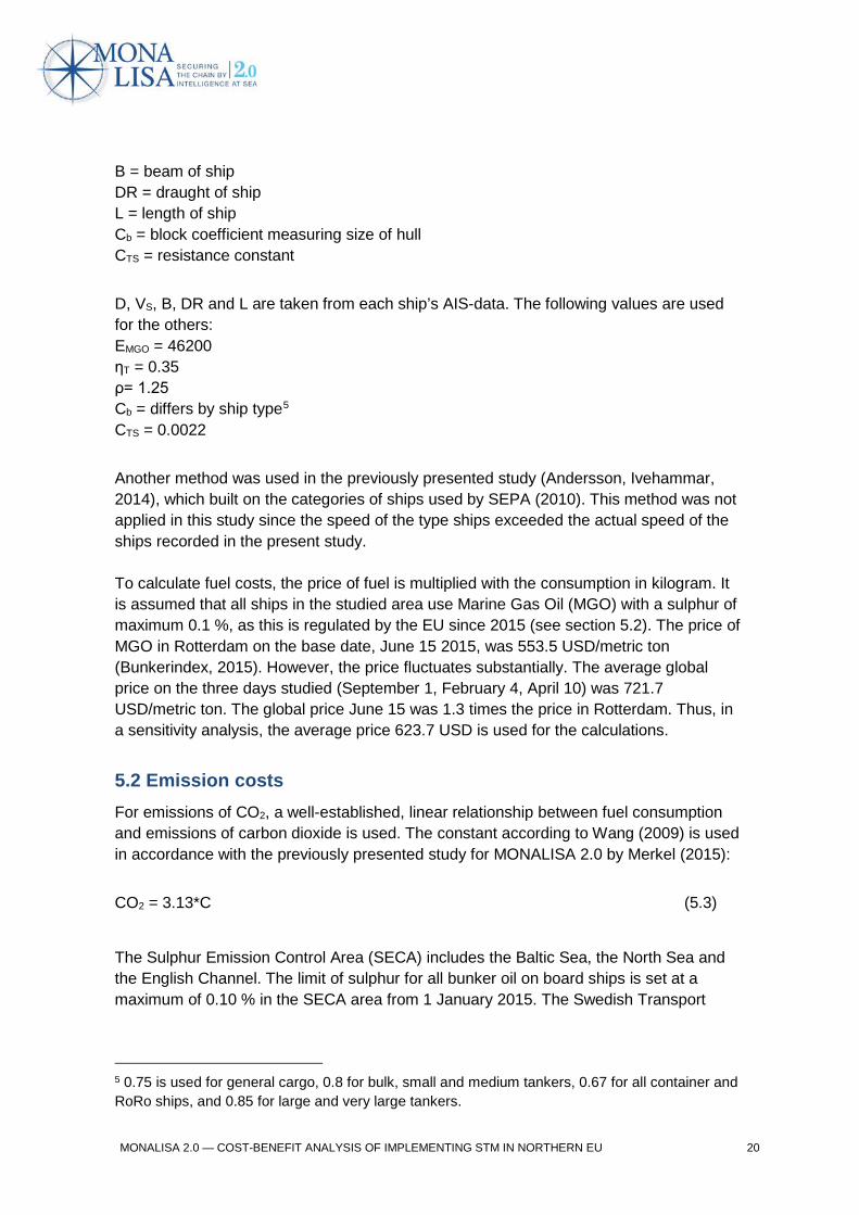
D, VS, B, DR and L are taken from each ship’s AIS-data. The following values are used for the others: EMGO = 46200 ηT = 0.35 ρ= 1.25 Cb = differs by ship type5 CTS = 0.0022

Another method was used in the previously presented study (Andersson, Ivehammar, 2014), which built on the categories of ships used by SEPA (2010). This method was not applied in this study since the speed of the type ships exceeded the actual speed of the ships recorded in the present study. To calculate fuel costs, the price of fuel is multiplied with the consumption in kilogram. It is assumed that all ships in the studied area use Marine Gas Oil (MGO) with a sulphur of maximum 0.1 %, as this is regulated by the EU since 2015 (see section 5.2). The price of MGO in Rotterdam on the base date, June 15 2015, was 553.5 USD/metric ton (Bunkerindex, 2015). However, the price fluctuates substantially. The average global price on the three days studied (September 1, February 4, April 10) was 721.7 USD/metric ton. The global price June 15 was 1.3 times the price in Rotterdam. Thus, in a sensitivity analysis, the average price 623.7 USD is used for the calculations.

5.2 Emission costs For emissions of CO2, a well-established, linear relationship between fuel consumption and emissions of carbon dioxide is used. The constant according to Wang (2009) is used in accordance with the previously presented study for MONALISA 2.0 by Merkel (2015):

CO2 = 3.13*C (5.3)

The Sulphur Emission Control Area (SECA) includes the Baltic Sea, the North Sea and the English Channel. The limit of sulphur for all bunker oil on board ships is set at a maximum of 0.10 % in the SECA area from 1 January 2015. The Swedish Transport

5 0.75 is used for general cargo, 0.8 for bulk, small and medium tankers, 0.67 for all container and RoRo ships, and 0.85 for large and very large tankers.


Agency is the surveying authority for controlling that the sulphur content in the bunker oil fulfils the requirements. (The Swedish Transport Agency, 2015)

When we calculate emissions of nitrogen oxides (NOX), sulphur dioxide (SO2) and particulate matter 2.5 (PM2.5) we use the emissions per kg fuel for different categories in SEPA (2010). The emissions depend on ship types and thus ship types are considered for the calculations (individually or as categories). Table 5.1 shows emissions of NOX, SO2 and PM2.5 per kg fuel, assuming that all ships are driven by MGO with a sulphur of maximum 0.1 %.

Table 5.1 Kg emissions of NOx, SO2 and PM2.5 per kg fuel, categories of ships

Source: Table 12, SEPA (2010), adjusted for shifting to MGO

There are different recommendations of which unit values should be used for cost-benefit calculation and analysis in the transport sector, and it was decided that calculations be based on three such recommendations: ASEK, CAFE and the Stern Review. ASEK is a project in Sweden, led by the Swedish Transport Administration which, based on research, recommends which methods and unit values should be used for cost-benefit calculation and analysis in the transport sector in Sweden. SEPA (2010) uses the values from ASEK 4 (SIKA, 2009) as main values to calculate emission costs for different types of ships. As alternative values SEPA (2010) uses values from the European Union’s program for clean air called Clean Air for Europe (CAFE) (EC DG Environment, 2005) and from the Stern Review on the Economics of Climate Change (Stern, 2006). The Stern report discusses the effects on the world economy of global warming.

The last ASEK recommendations are ASEK 5, from 2014 (The Swedish Transport Administration, 2014). The recommended values for calculating emission costs according to ASEK 5 in 2010 prices are 80 SEK per kg NOX and 27 SEK per kg SO2. (The Swedish

Ship type NOX SO2 PM2.5 Cargo small 0.0731 0.00180 0.00119 Bulk medium 0.0728 0.00170 0.00115 Bulk large 0.0729 0.00172 0.00116 RoRo (incl automobile) 0.0661 0.00191 0.00125 Container medium 0.0733 0.00184 0.00122 Container large Container very large 0.0722 0.00156 0.00108 Tanker small 0.0731 0.00180 0.00119 Tanker medium 0.0728 0.00170 0.00115 Tanker large 0.0734 0.00181 0.00134 Tanker very large 0.0734 0.00181 0.00134


Transport Administration, 2014) For CO2 the recommendation by ASEK 5 is 1.08 SEK per kg for the medium term.6 For sensitivity analysis ASEK 5 recommends 3.50 SEK per kg.

We will use the unit values recommended by ASEK 5 converted to euros and the price level for 2015 as the main alternative for the present report. As a low and a high alternative in a sensitivity analysis, we will use values used by SEPA (2010), Stern or CAFE converted into euros and the price level for 2015. When applicable, we use the values from ASEK for the Baltic Sea, as they are chosen to reflect the costs in waters near Sweden. For the North Sea, we use values from CAFE. The values in the two areas differ because more populated areas are affected by the emissions in the North Sea. For PM2.5 no values are estimated by ASEK, hence CAFE is used as the only source. Concerning emissions of carbon dioxide, the costs are globally distributed and the same values for the Baltic Sea and the North Sea are used. The values used are shown in Table 5.2.

Table 5.2 Values euro/kg and source for unit values used in the calculations, price level 2015

Main low high CO2 BS/NS 0.12 (ASEK) 0.07 (Stern, low) 0.35 (ASEK, high) NOX BS 9.01 (ASEK) 2.86 (CAFE low) 9.01 (ASEK)

NS 9.00 (CAFE average) 5.28 (CAFE low) 14.49 (CAFE high) SO2 BS 3.04 (ASEK) 3.04 (ASEK) 11.50 (CAFE high)

NS 12.94 (CAFE average) 7.14 (CAFE low) 20.70 (CAFE high) PM2.5 BS 21.50 (CAFE average) 12.42 (CAFE low) 36.22 (CAFE high)

NS 49.68 (CAFE average) 28.98 (CAFE low) 82.80 (CAFE high)

5.3 Manning costs The actual number of positions on board varies not only between the smaller and larger ships. It also differs for a similar size of ship due to age, condition, special requirements, nationality, etc. Manning costs were studied in a report for the Swedish Department of Industry (Andersson and Forsblad 2010) on the competitiveness of the Swedish shipping industry. The manning costs used in this report are based on that report.7 First, for each of the eleven types of ships, the number of positions (officers, mates) were estimated, based on the above mentioned report. ‘Officers’ include all superior positions on deck and

6 This is lower than the recommendation by ASEK 4, which was 1.50 SEK per kg CO2 in price level 2006. The Swedish Transport Administration (2014) mentions that in the EU Emissions Trading System the price per kg emissions of CO2 has been 0.30 SEK at its highest and most of the time even lower, and the HEATCO recommendation is 0.30 SEK per kg CO2 in price level 2010. However, The Swedish Transport Administration does not recommend those lower values. 7 Andersson and Forsblad (2010) obtained information about number of positions and labour costs from interviews and written material from most Swedish ship owners. Complimentary information about the number of positions was received in e-mails from large Swedish ship owners when making the previous study (Andersson, Ivehammar, 2014).


engine (master, first and second officer etc.) and ‘mates’ all other positions on deck, engine and for catering. The results are shown in Table 5.3. It must be noted that the categories are broad and the number of positions may vary substantially around the estimated average within each category. Table 5.3 Estimated number of positions for each type of ship

Ship type Estimated number of positions

Cargo small 4 officers, 5 mates Bulk medium 7 officers, 8 mates Bulk large 8 officers, 9 mates RoRo 8 officers, 9 mates Container medium 7 officers, 8 mates Container large 8 officers, 8 mates Container very large 9 officers, 10 mates Tanker small 6 officers, 6 mates Tanker medium 7 officers, 8 mates Tanker large 9 officers, 10 mates Tanker very large 9 officers, 11 mates

A particular problem with manning costs at sea is that seamen on ships registered in different countries normally are hired on the terms stated by agreements and labour laws made in each country. However, these differ substantially between countries. Normally when evaluating labour costs in a cost-benefit analysis, it is assumed that the alternative value is the gross (total) cost for the employer including payments for income tax and for social benefits, because it is the value of what the employee is expected to produce in the best alternative employment. However, in high cost countries in the west, this is not usually the case because in order to have a competitive wage compared to low-cost countries, the public sector subsidizes the shipping companies and reimburses income tax and payments for social benefits. In that case, the theoretically correct cost, i.e. the value of the foregone employment for the seamen concerned, is the net wage.

A second problem is that crewmembers are not always employed full time. Under many Western European contracts, there are two persons employed full time per position. Taking into account some extra need for persons owing to vacation and other reasons for vacancies, it is possible to estimate that there is a need for about 2.1 persons per position. However, many crewmembers, especially mates, are hired on temporary contracts. Then there will only be one person employed full time per position. In order not to underestimate costs, in the main alternative it is assumed that for officers the total cost is 2.1 times the monthly net wage. For mates, a mix between low cost wages and western contracts is assumed. Thus, to construct a reasonable average, the wage is multiplied by a factor 1.5 in order to make it an average between different types of employment conditions.


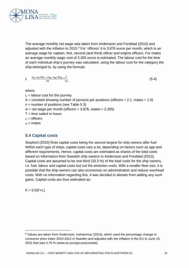
The average monthly net wage was taken from Andersson and Forsblad (2010) and adjusted with the inflation to 2015.8 For ‘officers’ it is 3,876 euros per month, which is an average wage for captain, first, second (and third) officer and engine officers. For mates an average monthly wage cost of 2,305 euros is estimated. The labour cost for the time of each individual ship’s journey was calculated, using the labour cost for the category the ship belonged to, by using the formula:

𝐿𝐿 = 𝐴𝐴𝑀𝑀(𝑛𝑛𝑀𝑀∗𝑊𝑊𝑀𝑀)+𝐴𝐴𝑀𝑀(𝑛𝑛𝑀𝑀∗𝑊𝑊𝑀𝑀)30

* 𝑇𝑇24

(5.4)

where L = labour cost for the journey A = constant showing number of persons per positions (officers = 2.1, mates = 1.5) n = number of positions (see Table 5.3) w = net wage per month (officers = 3,876, mates = 2,305) T = time sailed in hours O = officers M = mates

5.4 Capital costs Stopford (2010) finds capital costs being the second largest for ship owners after fuel. Within each type of ships, capital costs vary a lot, depending on factors such as age and different requirements. Hence, capital costs are estimated as shares of the total costs based on information from Swedish ship owners to Andersson and Forsblad (2010). Capital costs are assumed to be one third (33.3 %) of the total costs for the ship owners, i.e. fuel, labour and capital costs but not the emission costs. With a smaller fleet size, it is possible that the ship owners can also economize on administration and reduce overhead costs. With no information regarding this, it was decided to abstain from adding any such gains. Capital costs are thus estimated as:

K = 0.5(F+L)

8 Values are taken from Andersson, Ivehammar (2014), which used the percentage change in consumer price index 2010-2012 in Sweden and adjusted with the inflation in the EU to June 15, 2015 that was 4.76 % (www.ec.europa.eu/eurostat).


6. Benefits of route optimisation

6.1 Total costs for sea traffic in the northern part of the EU Using all the sea traffic that was recorded by AIS data and described in chapter 3 together with the costs for shipping companies and the costs for emissions presented in chapter 5, the total cost to society per year of sea traffic for cargo ships and tankers above 60 meters and 300 GT in the studied area can be estimated. This calculation is based on the (1,944 + 1,111) = 3,055 ships which were observed during the three days. To obtain annual costs, the costs for three days are multiplied by 120, assuming that the three days are representative for sea traffic in one year. Table 6.1 shows the number of ships in each category for the Baltic Sea and for the North Sea, as well as costs distributed between different categories. Fuel costs are calculated using the fuel price of 553 USD from the base day June 15 converted into euros with the exchange rate 1.12 USD/EUR. Table 6.1 Total annual costs to society for ship traffic in the northern part of the EU, million euros

When both areas are added, it results in an annual cost to society for all sea traffic with cargo ships and tankers in the northern part of the EU of 3,674 million euros. Large bulkers and tankers, owing to high fuel consumption, represent the category with the highest costs, especially in the North Sea. Small cargo ships is the most common category but represents only 13 % of the total costs in the Baltic Sea and 5 % in the North Sea. Cargo ships contribute with 70 % of the total costs in the Baltic Sea and 75 % of total costs in the North Sea.

Baltic Sea North Sea Ship type Number

ships

Costs million EUR

Number ships

Costs million EUR

cargo Cargo small 843 271 393 75 Bulk medium 98 111 68 53 Bulk large 167 402 143 677 RoRo (incl automobile) 113 184 68 114 Container medium 129 173 66 59 Container large 92 223 70 111 Container very large 7 33 34 95

tanker Tanker small 181 92 98 136 Tanker medium 64 118 45 32 Tanker large 242 453 114 213 Tanker very large 8 30 13 19

Total 1,944 2,089 1,111 1,585


The cost per ship is lower for the smaller ships and increases with size for all types of ships. For example, the cost to society for a small cargo ship’s traffic in the Baltic Sea area in a year is 320,000 euros compared to 2.4 million euros for the large bulkers in the area; 507,000 euros for a small tanker and 1.9 million for a large tanker. However, the fact that the cost is lower for small ships does not mean that they are the most efficient, because at the same time they carry less cargo.

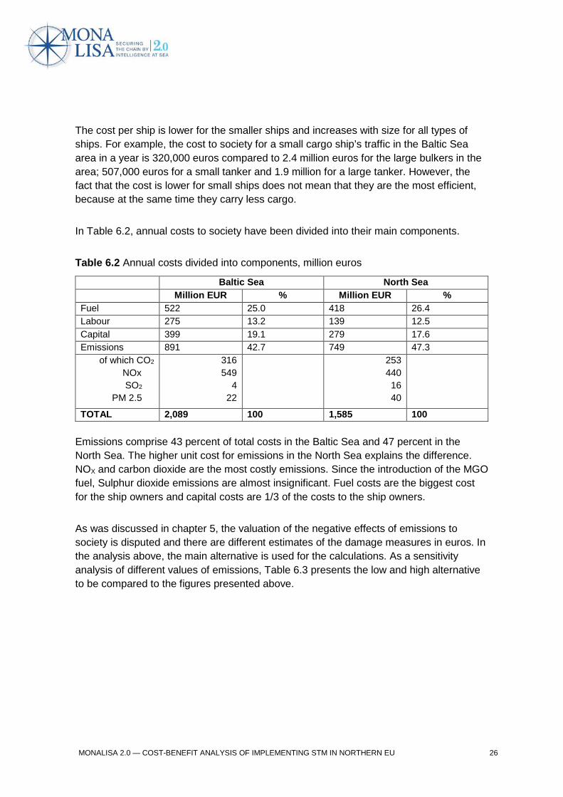
In Table 6.2, annual costs to society have been divided into their main components.

Table 6.2 Annual costs divided into components, million euros

Baltic Sea North Sea Million EUR % Million EUR % Fuel 522 25.0 418 26.4 Labour 275 13.2 139 12.5 Capital 399 19.1 279 17.6 Emissions 891 42.7 749 47.3

of which CO2 NOx SO2 PM 2.5

316 549

4 22

253 440 16 40

TOTAL 2,089 100 1,585 100 Emissions comprise 43 percent of total costs in the Baltic Sea and 47 percent in the North Sea. The higher unit cost for emissions in the North Sea explains the difference. NOX and carbon dioxide are the most costly emissions. Since the introduction of the MGO fuel, Sulphur dioxide emissions are almost insignificant. Fuel costs are the biggest cost for the ship owners and capital costs are 1/3 of the costs to the ship owners.

As was discussed in chapter 5, the valuation of the negative effects of emissions to society is disputed and there are different estimates of the damage measures in euros. In the analysis above, the main alternative is used for the calculations. As a sensitivity analysis of different values of emissions, Table 6.3 presents the low and high alternative to be compared to the figures presented above.


Table 6.3 Sensitivity analysis: annual costs divided into components, million euros

Low alternative High alternative Baltic Sea North Sea Baltic Sea North Sea Million

EUR % Million

EUR % Million

EUR % Million

EUR %

Fuel 522 33.2 418 32.8 522 19.2 418 17.6 Labour 275 17.5 139 10.9 275 10.1 139 5.9 Capital 399 25.4 279 21.9 399 14.7 279 11.7 Emissions 376 23.9 438 34.4 1,526 56.0 1,539 64.8

of which CO2

185

148

923

739

NOx 174 258 549 708 SO2 4 9 17 25

PM 2.5 13 23 37 67 TOTAL 1,573 100 1,274 100 2,723 100 2,375 100 In % of main alternative

75.3

80.4

130.4

149.8

When all the low unit values for emissions are applied, the total cost to society becomes 25 percent lower in the Baltic Sea and 20 percent lower in the North Sea. The total cost falls from 3,674 million to 2,847 million euros. The smaller reduction in the North Sea comes from a lower difference in unit values for this area. If all unit values in the high alternative are applied instead, the total cost becomes 30 percent higher in the Baltic Sea and almost 50 percent higher in the North Sea, totalling 5,098 million euros.

The ambiguity in how to value emissions is clearly illustrated, by the total emission cost in the Baltic Sea varying between 376 and 1,576 million euro and between 438 and 1,539 in the North Sea. Consequently, the share of emission costs of total costs varies between 24 and 56 percent for the Baltic Sea and between 34 and 65 percent for the North Sea. In should be noted, however, that this is the largest possible interval, as it is a combination of either all the lowest or all the highest values of emissions.

As emission costs are a major cost component, it also contributes with the largest insecurity. Several other sensitivity analyses are carried out. Another significant cost driver is the price of fuel, which varies substantially over time. If the average price for the studied three days is used instead of the spot price of 553.5 USD/tonne from June 15, the total cost would increase by four percent. If, however, it is assumed that the fuel price is 50 percent higher, the total cost to society would increase 19 percent.

Alternative assumptions concerning labour and capital will change the total cost with less than ten percent. If for example one more person per position for officers and for mates for all categories of ships is assumed, the total cost to society would increase by just over one percent. If it instead had been assumed that there was only one person employed per position (instead of 2.1 for officers and 1.5 for mates), meaning that all employees are on temporary contracts, the total cost to society would fall by 4 %. If capital costs were 40


percent of ship owner’s cost instead of 33.3 percent, the total cost would go up by approximately six percent. Thus, other costs than those for emissions and fuel contribute relatively little to the uncertainty.

6.2 The potential for route optimization How much ships will be able to shorten their route depends on many factors. The resulting average distance per ship that can be saved consists of many ships that may not shorten their route at all and ships that under certain conditions may save several percent. There are several possibilities to obtain such savings.

One option is to “cut corners” along today’s routes when there is no conflicting traffic in the opposite direction. If ships are informed about the intended route of other ships in the vicinity it will make it easier to shorten routes without jeopardizing safety. This option can be enhanced with the support of flow management from a monitoring central ashore. The study from SSPA (2015) conducted simulations of the traffic in the Sea of Kattegat, which is a particular area with a lot of traffic in crossing fairways and one large corner where the traffic could take a shorter route with the help of STM. The study finds that in one month, it is possible to reduce fuel consumption with 10.8 percent by optimising routes. This corresponds approximately to three times the reduction of distance. The unit values presented in chapter 5 are applied to calculate the benefit to society of this optimization. Without exact knowledge about the types of ships are involved, an average of the different emission factors for different ship types is used. If the traffic in the Sea of Kattegat has the same composition of ships as in the Baltic Sea in general, this will be a correct estimation. The saving for the month of August 2014 was 4.6 million euros, of which 37 percent is reduced fuel costs and the remaining 63 percent are reduced costs for emissions. For a whole year, the savings to society including the reduced emissions from route optimization in the area is 55 million euros, if the unit values from the present study are applied to this simulation.

Today’s traffic is typically separated by 7-10 kilometres in opposite direction. Ships sail at 20-40 km/h. This can be compared with airplanes, which fly at around 900 km/h and is separated by ten kilometres horizontally or 330 meters vertically. In narrow waters, separation becomes smaller, and in fairways in ports, channels and archipelagos, ships meet with even smaller margins. In order to quantify the importance of reducing the sailed distance along separated zones, another set of AIS data from the Swedish Maritime Administration is used. It consists of the traffic crossing certain passage lines during the month of April 2015. One was drawn in the strait Bälten, one in Öresund south of Malmö and one between Bornholm and Sweden, ‘Bornholmsgattet’. Ships were separated, using the course registered in AIS-data when crossing the line, between those sailing inbound to and outbound from the Baltic Sea. The results are shown in table 6.4.


Table 6.4 Average number of ships per day passing lines in the Baltic Sea, April 2015

Inbound Outbound Total

Bälten 14.7 25.9 40.6

Öresund 33.7 24.4 58.1

Bornholmsgattet 56.3 57.8 114.1

An analysis is made of ships first passing inbound to the Baltic Sea either through Bälten or Öresund and subsequently passing at Bornholmsgattet. Inbound ships sail a 5-7 percent longer distance than outbound between these lines. On average, 24.6 ships per day sailed from Öresund to Bornholmsgattet and another 6.5 per day from Bälten to the same line. The total of 31.1 ships make 3.8 percent of the average daily number of ships registered in the data presented in chapter 3, and represent 3.5 percent of the total sailed distance in that area. If the inbound traffic owing to route optimisation could take a five percent shorter route on average without reducing safety, near 0.2 percent of the total cost in the Baltic Sea would be saved. Other separated areas may contribute to additional gains in terms of shorter distances.

With the modern technology that STM provides, it appears plausible that with optimised routes in the entire area, ships on average would be able to sail at least one percent shorter than under previous conditions. Those gains may consist of zero percent in some areas and several percent in other areas.

6.3 Benefits of shorter routes There are two ways to take advantage of the possibility to shorten distance. One alternative is to sail at constant speed arriving earlier to the port and be able to load or unload prior to the time of arrival without route optimisation. Choosing this alternative, ship owners can save on fuel, labour and capital, and additionally, the transit time of the cargo falls. Since the total costs for cargo and tanker traffic in the northern part of the EU in the main alternative is approximately 3,700 million euros, 37 million euros per year can be saved on fuel, labour and capital for each percentage that ships can reduce the sailed distance when sailing with constant speed.

The other alternative is to utilize the shorter route to reduce speed and arrive at the same time as with the longer route. With such slow steaming, savings are only in the form of lower fuel consumption and resulting reduction of emissions. In Table 6.5, the benefit to society if speed is reduced instead of the time sailed is shown.


Table 6.5 Benefits to society for reduction in speed, million euros per year

Saved distance Baltic Sea North Sea Total

0.1 % 4.2 3.5 7.6

0.5 % 20.8 17.4 38.2

1 % 41.4 34.7 76.1

2 % 81.9 68.7 150.6

5 % 198.6 166.6 365.2

If the distance is shortened by one percent, the gain to society would be 76.1 million euros per year if ships’ speed is reduced, compared to 37 million euros (not counting benefits of decreased transit times of the cargo) in the case where speed is held constant.


7. Benefits of adjusted arrival times

7.1 Methodology for calculating the benefits Instead of lying at anchor and wait for berth, ships can decrease speed. The saving from decreased speed due to adjusted arrival times based on better updated information about berthing times will be reduced fuel consumption, which will lower fuel costs as well as emission costs.

The amount of saved fuel depends on how many hours before arrival a ship can reduce its speed in order to save fuel. This, in turn, depends on how long before berthing ports would be able to provide reliable information about berthing time and for how long before berthing ships currently lie at anchor, as well as the reduction in speed.

Fuel consumption per hour in kg for a specific ship is calculated as

𝐶𝐶ℎ = 𝐶𝐶𝑚𝑚 ∗ 𝑆𝑆𝑘𝑘ℎ ∗ 1852 (7.1)

where Ch= fuel consumption per hour for the ship Cm= fuel consumption per metre for the ship calculated with equation (1) and (2) with D=1 Skh=speed in knots per hour

Saved fuel due to adjusted arrival time for a ship is calculated as

𝐶𝐶𝑠𝑠𝑠𝑠 = �(𝐶𝐶ℎ0 ∗ ℎ𝑠𝑠𝑠𝑠) − �𝐶𝐶ℎ1 ∗ℎ𝑠𝑠𝑠𝑠

(1−𝑠𝑠𝑠𝑠)�� (7.2)

where Csa= saved fuel consumption for the ship Ch0= fuel consumption per hour at the sailed speed Ch1= fuel consumption per hour at decreased speed hsl= hours before the original ETA (estimated time of arrival) starting to slow down speed sr= relative speed reduction

The hours before original ETA (estimated time of arrival) it is possible for the ship to start

to slow down and save fuel is restricted by

ℎ𝑠𝑠𝑠𝑠 ≤ ℎ𝑖𝑖𝑛𝑛, ℎ𝑠𝑠𝑠𝑠

(1−𝑠𝑠𝑠𝑠) ≤ (ℎ𝑖𝑖𝑛𝑛 + ℎ𝑠𝑠𝑛𝑛) (7.3)


where

hin= hours in advance of original ETA the information can be received

han= hours the ship was anchored awaiting berth

The emissions of CO2 are calculated as 3.13 kg per kg fuel and PM2.5 as 0.0012 per kg

fuel. Table 7.1 shows the values for the block coefficient (Cb)9 and the emissions per kg

fuel that differs with ship type for the six categories of ships.

Table 7.1 Values that differ with ship type

Ship type GT interval Cb NOx/kg fuel SO2/kg fuel Cargo, small 100–5,999 0.75 0,071 0,0018 Cargo, medium 6000–13,999 0.75 0,073 0,0017 Cargo, large ≥14,000 0.75 0,073 0,0017 Tanker, small 100–5999 0.825 0,0731 0,0018 Tanker, medium 6,000–13,999 0.825 0,0731 0,0018 Tanker, large ≥14,000 0.825 0,0732 0,0018

7.2 Benefits of adjusting arrival times The saved fuel is calculated for each anchored ship and summed to a total fuel saving per year under different assumptions. Table 7.2 shows the saved fuel if speed is reduced by 10 percent, 25 percent or 50 percent and the possible time in advance the information can be received is one hour, four hours or 12 hours prior to the original ETA for the ship.

Table 7.2 Fuel savings in 1000 kg per year from adjusted arrival times in the Baltic Sea Region

Time prior to arrival information is provided Reduction in speed 1 hour 4 hours 12 hours 10 % 807 3,218 9,672 25 % 1,864 7,433 22,252 50 % 5,139 12,154 33,881

Table 7.3 shows the saved emissions in thousand kilos of SO2, NOX and PM 2.5, while

Table 7.4 shows the saved emissions of CO2.

9 For simplicity, the values for Cb in this section is the average of the one for cargo ships and for tankers


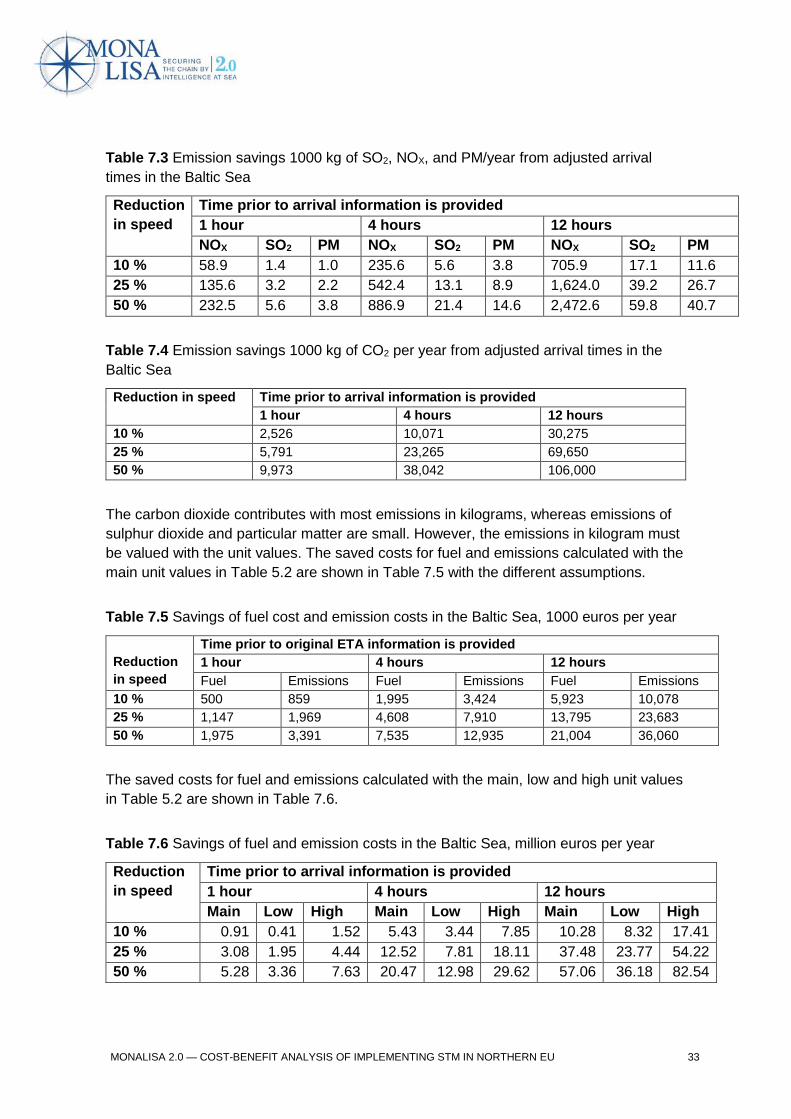
Table 7.3 Emission savings 1000 kg of SO2, NOX, and PM/year from adjusted arrival times in the Baltic Sea

Reduction in speed

Time prior to arrival information is provided 1 hour 4 hours 12 hours NOX SO2 PM NOX SO2 PM NOX SO2 PM

10 % 58.9 1.4 1.0 235.6 5.6 3.8 705.9 17.1 11.6 25 % 135.6 3.2 2.2 542.4 13.1 8.9 1,624.0 39.2 26.7 50 % 232.5 5.6 3.8 886.9 21.4 14.6 2,472.6 59.8 40.7

Table 7.4 Emission savings 1000 kg of CO2 per year from adjusted arrival times in the Baltic Sea

Reduction in speed Time prior to arrival information is provided 1 hour 4 hours 12 hours

10 % 2,526 10,071 30,275 25 % 5,791 23,265 69,650 50 % 9,973 38,042 106,000

The carbon dioxide contributes with most emissions in kilograms, whereas emissions of sulphur dioxide and particular matter are small. However, the emissions in kilogram must be valued with the unit values. The saved costs for fuel and emissions calculated with the main unit values in Table 5.2 are shown in Table 7.5 with the different assumptions.

Table 7.5 Savings of fuel cost and emission costs in the Baltic Sea, 1000 euros per year

Reduction in speed

Time prior to original ETA information is provided 1 hour 4 hours 12 hours Fuel Emissions Fuel Emissions Fuel Emissions

10 % 500 859 1,995 3,424 5,923 10,078 25 % 1,147 1,969 4,608 7,910 13,795 23,683 50 % 1,975 3,391 7,535 12,935 21,004 36,060

The saved costs for fuel and emissions calculated with the main, low and high unit values in Table 5.2 are shown in Table 7.6.

Table 7.6 Savings of fuel and emission costs in the Baltic Sea, million euros per year

Reduction in speed

Time prior to arrival information is provided 1 hour 4 hours 12 hours Main Low High Main Low High Main Low High

10 % 0.91 0.41 1.52 5.43 3.44 7.85 10.28 8.32 17.41 25 % 3.08 1.95 4.44 12.52 7.81 18.11 37.48 23.77 54.22 50 % 5.28 3.36 7.63 20.47 12.98 29.62 57.06 36.18 82.54


To choose a main alternative, assumptions must be made about what is a reasonable time before ETA that the reliable information can be received by the (master of) the ship that no more changes are likely, and for how long time a typical ship sails between ports. The AIS data for the Baltic Sea (Chapter 3) shows that some ships do not sail far between two ports in the Baltic Sea. A 25 percent speed reduction and information four hours or twelve hours before original ETA is estimated as reasonable alternatives. Thus benefits are between 12.52 million euro and 37.48 million euro. How the savings in the main alternatives are distributed on the different ship types if all reduced speed accordingly is shown in Table 7.7.

Table 7.7 Total savings, main values, information received 4 hours or 12 hours before original ETA, 25 % reduction in speed, categories of ships

Ship type GT interval Savings 1000 euros 4 hours 12 hours Cargo, small 100–5,999 726 2,101 Cargo, medium 6000–13,999 1,656 4,967 Cargo, large ≥14,000 2,959 8,876 Tanker, small 100–5999 998 2,994 Tanker, medium 6,000–13,999 1,609 4,826 Tanker, large ≥14,000 4,571 13,714 Total 12,519 37,478


8. Costs for the project In this chapter, an outline of the costs associated with the Sea Traffic Management (STM) concept is presented. As the concept is still in a development phase, all costs have to be estimated based on current knowledge and reasonable assumptions. The figures presented in this chapter are estimates given by different persons at a MONALISA 2.0 project meeting (MONALISA 2015) or later in mails to the authors, and are not the author’s unless clearly stated. Investments are assumed to depreciate during eight years. Investment costs may fall over time as technology develops, but in order not to underestimate the costs and make the project appear profitable, relatively high estimates of the costs are used. It is unlikely that STM would be introduced only in the northern part of the EU. As many ships involved operate outside of the studied area, it would be an overestimation to allocate all investment costs for the project to this area. We have allocated 50 percent of the investment costs that are not specific to this area to the project. Since the costs are uncertain, we will present a higher alternative and a lower alternative when estimating the costs for the project.

STM will give raise to costs for the ships involved, i.e. for the ship owners; for the ports involved and for the private businesses or public authorities who are providing the services. In the following, we estimate the costs for the studied areas in the Baltic and North Sea. If STM is applied in the whole of the EU, ships that operate in the northern parts of the EU have already installed necessary equipment and the additional cost for implementing STM on a broader scale will not increase proportionally.

8.1 Costs related to the ships In 2013 around 5,000 unique ships of the types in this study sailed in the entire Baltic Sea of which around 75 percent are cargo ships and 25 percent are tankers (Swedish Institute for the Marine Environment, 2014). There are no corresponding figures for the area in the North Sea that we study, but as most ships that operate in the Baltic Sea also operate in the North Sea, and the present study do not cover the entire Baltic Sea, it is assumed that the total number of unique ships totally in the studied area is 5,000.

Ships have to make investments in the technology required and also in training for the staff who are going to run the equipment. It is estimated that the annual costs for a ship’s required equipment for participating is 1,500 euros. With 5,000 ships in the area, the total investment cost is around 7.5 million euros per year. 50 percent of this cost is allocated to the project, i.e. 3.75 million euros per year.

Today’s staff needs to be trained. It is estimated that additional training for the system will amount to between 1,000 euros per person for a two-day course, and 500 euros for a one-day course and that training is required for on average six persons per ship. With 5,000 ships in the area, a once-and-for-all investment in training of between 15 and 30 million euros is needed. This cost is expected to disappear in the longer run when the


training will be included in the regular education of ship officers. If the cost is distributed over ten years with a discount rate of 3.5 percent, 50 percent of the annual cost is between one and two million euros.

Ships applying STM will exchange information with other ships and stations ashore. The annual cost for this communication has been estimated at on average 2,300 euros per ship and year as the higher alternative and 1,150 as the lower. In the studied area, there were on average 648 cargo ships and tankers per day operating in the Baltic Sea and 371 ships in the North Sea. Some other ships like ferries will also be using the services. It is estimated in cooperation with providers of the technology that the daily number of ships applying STM in the study area to 1,100. The communication cost per year will then end up at between about 1.25 and 2.5 million euros. 8.2 Costs related to the ports To apply Port CDM, investments in equipment must be made in the ports. The need to invest can be expected to vary depending on the size of the port. When implemented, it will make it possible for ships to adjust arrival times and to make port operations more efficient. Complete Port CDM is estimated to require investments of the magnitude of 100,000-200,000 euros in the high alternative.

However, not all ports need to implement such extensive application of Port CDM. From the study of anchored ships, it can be concluded that in the studied area in the Baltic Sea Region, only seven ports have on average at least one ship that arrived and had to anchor before berthing per day and 86 EU harbours in the area had at least one anchored ship waiting for berth in the harbour. Thus, there are many ports with less intense traffic that not require the extensive application of Port CDM.

In the high alternative it is assumed that seven big ports with most anchored ships in the Baltic Sea Region, that are identified in our study, make the full investment of on average 150,000 euros, another 20 medium sized ports invest 75,000 euros and the remaining ports invest 10,000 euros. In addition to investments are the costs for running the system. They are assumed to be 10,000 euros per year in the big ports, 5,000 euros per year in the medium sized ports and 1,000 euros per year in the remaining ports. It is estimated that the annual cost for investments and running the system in the seven big ports is 25,000 euros, for the twenty medium sized is 12,500 euros and for another 30 is 2,500 euros per year. The total costs for implementing Port CDM in the Baltic Sea would under these assumptions sum up to half a million per year in the high alternative.

In the low alternative the only costs assumed are for the adaptation that each actor is required to make in order to capitalize on PortCDM functionality by building connectors allowing the PortCDM integration platform to extract information, expected to be 1000 euros per connector at approximately 15 connectors per port in average. Counting the big and the medium sized ports this sums up to approximately 200 000 euros per year.


8.3 Costs for governance Applying the concept of STM internationally prerequisites that the system is governed by national and/or international bodies. For the entire EU, it is estimated that the governance costs would amount to 5 million euros per year. 50 percent of this cost is allocated to the project, resulting in an annual cost of 2.5 million euros.

To apply flow management and obtain the full benefits of route optimization (analysed in chapter 6), there would be public or private service providers doing optimization as well as monitoring services ashore. These can be regarded as open-sea versions of today’s VTS (Vessel Traffic Service) monitoring the traffic in ports and archipelagos. SoundREP in the Sound between Sweden and Denmark is one current example of such a central. It is assumed that there would be seven such centrals: five in the Baltic Sea and two in the North Sea. It is estimated that each central would have to make investments of the same magnitude as the biggest ports, i.e. around 150,000 euros. Each position in the central to conduct Flow Management would require seven employees, covering 24 hours monitoring all year around. It is assumed that each person costs 60,000 euros, based on today’s costs for VTS staff. Each position would bring about costs of 2.5 million euros per year. It is assumed that there are two positions in each central, this would add up to 84 persons in the seven centrals.

The study of STM is not a comparison between an implemented STM and today’s situation, but a comparison between with and without STM in the future. If new technology is implemented only with STM it might ease the workload for today’s VTS operators and if STM is implemented, there would be fewer such operators needed. In the low alternative it would be assumed that today’s VTS operators can handle all the tasks.

The total annual cost would be about 125,000 euros for investments and 5 million euros for staff in the higher alternative and no extra cost for staff in the lower alternative, thus adding to between 0.125 and 5.125 million euros per year. 8.4 Summary of estimated costs The costs in the higher and in the lower alternative are summarized in Table 8.1.


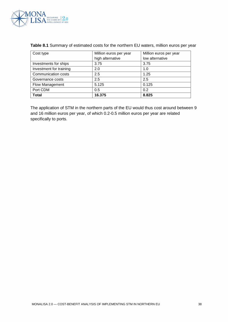
Table 8.1 Summary of estimated costs for the northern EU waters, million euros per year

Cost type Million euros per year high alternative

Million euros per year low alternative

Investments for ships 3.75 3.75 Investment for training 2.0 1.0 Communication costs 2.5 1.25 Governance costs 2.5 2.5 Flow Management 5.125 0.125 Port CDM 0.5 0.2 Total 16.375 8.825

The application of STM in the northern parts of the EU would thus cost around between 9 and 16 million euros per year, of which 0.2-0.5 million euros per year are related specifically to ports.


9. Case study: The benefits of Port CDM in the Port of Gothenburg

This chapter is a summary of the study by Merkel (2015). It considers two major sources of benefits that are hypothesized to result from transitioning to collaborative port operations, where involved actors collaboratively through real-time sharing of information optimize the port approach and turnaround process. Locations, intentions and capabilities of terminal operators, service providers and ships are shared to ensure:

1) Higher predictability in estimated berthing times, giving rise to shortened time spent waiting for berthing by approaching the port at a more optimized speed.

2) Improved readiness of terminal operators and service providers in port,

resulting in shortened service times and total port turnaround times.

The estimation of impacts is based on one month’s traffic data in the Port of Gothenburg. The data used (SSPA, 2015) was collected and structured by Viktoria Swedish ICT, and is a detailed set of information regarding the port calls made to the Port of Gothenburg during the month of August, 2014. The information regards estimated times of arrival, actual arrival and departure at certain states in the port approach.

There are two separate benefit categories owing to the dynamic exchange of information

in the collaborative port:

• Voyage speed optimization prior to port approach, enabling operational and environmental cost savings.

• Shorter service times and subsequently shorter total port turnaround times, enabling operational, capital, time and environmental cost savings.

The benefit of voyage speed optimization is already captured by the anchoring study presented in Chapter 4 and Chapter 8. The number of ships in August 2014 is similar to, but somewhat lower than, the estimated number of ships anchoring before entering the port of Gothenburg in the study described in Chapter 4. Recalculated to one month the estimated number of anchored ships in the study presented in Chapter 4 would be 73 ships. The number of ships anchored before entering the port of Gothenburg in August 2014 was 55 (SSPA, 2015).

The study considers the effects of a fully implemented Port CDM concept in the Port of Gothenburg against a business-as-usual scenario. It is assumed that Port CDM is neutral with regard to changes in traffic safety. Therefore, neither effects of increased nor


decreased safety of operations are estimated. The estimated benefits of Port CDM by cost savings from reduced service times in the port of Gothenburg under different scenarios is shown in Table 9.1.

Table 9.1 Estimated annual benefits of reduced service time, million euros/year

Low-impact scenario Median-impact scenario High-impact scenario

5.87 14.67 23.47

The low-impact scenario assumes that service times can be reduced by 1 hour. The high-impact scenario assumes a service time reduction of 4 hours. The median-impact scenario assumes the average impact of the low and high cases, and a service time reduction of 2.5 hours. The estimated benefits are to a majority made up of emissions cost savings, capital cost savings and bunker cost savings. The most noteworthy source of uncertainty in the estimations according to Merkel (2015) is related to the size of the traffic sample, and its representativeness for long term flows of traffic in the Port of Gothenburg.

We have found no studies about the current efficiency in the port of Gothenburg and if there is a potential to improve it, and if so, with how much. This case study shows an important stage in the production process of sea transportation and the need to extend such studies to more ports. Before more evidence is provided, cautious conclusions about the potential gains must be made.


10. Cost-benefit analysis of Sea Traffic Management This report analyses three parts of STM: the effects of route optimization, adjusted arrival times and reduced service times in ports. In this chapter we present the cost-benefit analysis of more efficient sea transportation through the implementation of the STM concept, discuss the trade-off between efficiency and safety, and propose issues that need to be investigated further in order to validate the results.

10.1 Benefits and costs of route optimisation with constant safety The total costs for cargo and tanker traffic in the northern part of the EU, i.e. the main part of the Baltic Sea and the North Sea, were calculated in chapter 6. It was found that the total cost for society in the main alternative for the traffic was approximately 3,700 million euros per year of which around 45 percent are costs generated from emissions. Using all low and high unit values for emissions in the sensitivity analysis, costs range between 2,850 – 5,100 million euros. In the main alternative, this means that for each percentage that ships can reduce the distance approximately 37 million euros per year can be saved on fuel, labour and capital, with a maximum span of 29-51 million if operating with constant speed.

According to the present study, society will gain more if ships utilise the shorter distance by ‘slow steaming’, i.e. reducing speed instead of arriving earlier. Benefits to society includes all parties, thus both the savings for the ship owners and the gains from reduced emissions. If the benefit of decreased transit time of the cargo is not large, it would be more profitable for the ship owners to reduce speed, unless being restricted by contracts about arrival times.

The analysis shows that it will be beneficial for ship owners to participate in STM (reducing speed) if the distance can be shortened by 0.65 percent or more if they have to pay all costs for the project. It will be a net gain to society already if distances can be shortened by around 0.2 percent, when the effect on lower emissions is included, given that the estimation of costs is accurate. Thus, the conclusion from this cost-benefit analysis is that the break-even reduction in distance for making route optimisation profitable is 0.2 percent.

In Figure 10.1 the total savings for society, the savings for the ship owners in terms of reduced fuel consumption and the estimated costs for the project are compared for different percentages of shortened distance. As the system is not fully developed, costs can only be approximated. The estimates made by persons involved in the MONALISA project ended with plausible assumptions at around 16 million euros per year (see Chapter 8).


Figure 10.1 Benefits and costs of shortened distance

If the low or high alternatives for valuation of emissions are used instead of the main alternative, the savings will be 32 percent lower to 56 percent higher. The low, main and high alternatives are compared in Figure 10.2. Even if the low alternative to value emissions is applied, the net benefit will be positive if distances can be shortened by 0.5 percent. Figure 10.2 Benefits and costs of shortened distance, different valuation of emissions

Whether ships will reduce speed or arrive earlier is determined by several factors. The fuel savings for the ship is not the sole consideration for the ship owners: contracts

0

50

100

150

200

250

300

350

400

0,1 0,5 1 1,5 2 2,5 3 3,5 4 4,5 5

mill

ion

euro

s per

yea

r

saved distance in %

society saving

fuel saving

Cost

0

100

200

300

400

500

600

0,1 0,5 1 1,5 2 2,5 3 3,5 4 4,5 5

mill

ion

euro

s per

yea

r

saved distance in %

society saving

Cost

Savings society highalternative

Savings society lowalternative


specifying the ETA are one institutional constraint and requirements to be ready for loading or unloading to shorten transit time for cargo is another. Regardless of the choice, there will be a net gain to society if route optimization can shorten distances by at least around 0.5 percent. The case studies presented in section 6.2 appear to support that this is highly probable

10.2 Benefits and costs for Port CDM with adjusted arrival times Chapter 7 showed the costs for ships which arrive and having to anchor outside EU ports in the Baltic Sea. For adjusted arrival times, two factors determine the potential savings: how long before original ETA a ship is receiving reliable information and how much it reduces its speed. As a main alternative, it was assumed that ships reduce the speed by 25 percent. In one alternative, if speed reduction occurs 4 hours before ETA this would give rise to savings of 12.5 million euros per year. As another alternative, speed reduction can begin already 12 hours before ETA and savings would be 37.5 million euros. The potential savings depend on the assumptions about time and speed: a 10 percent speed reduction with information one hour before original ETA would only save 1 million euros and if all anchored ships would reduce speed by 50 percent and have information 12 hours before original ETA the savings would be as much as 57 million euros.

Additional savings may be possible within ports by implementing Port CDM in order to shorten turnaround times (service times). An alternative source of gains in ports, even if turnaround times remain unchanged, is a more efficient use of the port’s resources, which would in the long run reduce the demand for fixed capital as well as labour and hired resources in ports.

The case study from the port of Gothenburg summarized in chapter 9 illustrates the potential. The mean time spent at a quay in that port was 15 hours (Merkel, 2015). We present a one percent reduction of turnaround time as our main alternative, like for route optimisation, because to our knowledge there is no evidence proving the magnitude of inefficiencies in ports. For each percent that can be saved in the port, the turnaround time in the port of Gothenburg would be reduced by 9 minutes per ship. That would save 0.88 million euros per year. If all 7 ports in the Baltic Sea with most anchored ships could save the same amount, and another 20 could save 25 percent of that amount, the total gain to society would end up at around 10.6 million.

If the ships can reduce the time with one hour, as is assumed in one alternative by Merkel, it is equal to 6.7 percent shortened turnaround time in the port of Gothenburg. This would mean 5.9 million euros per year in benefit for society in a port of the size of Gothenburg and 71 million euros per year for the Baltic Sea with the same assumptions as above. This option is used as our high alternative.


As it remains to prove evidence of inefficiencies, we use 0 as our low alternative. This case study shows that the potential for savings with shared communication may be large, but is sensitive to assumptions about the actual saved turnaround time or saved resources, and additional studies are required to confirm the conclusions.

10.3 Additional benefits from increased safety with STM The analysis in the present study so far builds on the assumption that safety is unchanged and that the number of accidents is constant. Route optimisation and more effective means of monitoring ships intend to have a positive impact on safety. Unlike other measures, it aims at increasing safety not at the expense of longer routes, but at combining improved safety and efficiency.

In the study of the Sea of Kattegat, which is a particular area with many conflicting ships (referred to in section 6.2) routes were not only optimised, but through a Conflict Resolution Algorithm, the number of conflicts was reduced (SSPA 2015). In this simulation for August 2014, routes were shortened so 10.8 % of fuel consumption could be saved. At the same time, with optimized traffic, the number of conflict candidates (i.e. situations where ships could come into conflicting courses) was reduced with 60 percent, from today’s 337 to 138.

The benefit of higher safety should be added to the benefits from increased efficiency. SSPA (2015) uses data of present accidents in the area together with estimated increased safety from simulations and values of increased safety to calculate the benefit per ship year. The estimated value is 11,200 euro per ship year. A ship year is defined as a ship underway 24 hours per day for a year.

From the data presented in chapter 6.1 the estimated number of ship years in the Baltic Sea is 313 and in the North Sea is 141, totalling 454 ship years per year. Applying this estimate of the value of increased safety to the present study thus results in an additional benefit of 5.1 million euros per year.

10.4 Summary of benefits and costs The main results are summarised in Table 10.1. A main, a low and a high alternative are presented for different options to save with annual values in euros rounded up to millions.

• Route optimisation concerns the areas in the Baltic Sea and the North Sea

showed in figure 3.1 and 3.2 and savings from either arriving earlier or reducing

speed are presented. Low and high alternatives are different values of emissions.


• The gains from adjusted arrival times builds on the study of the entire EU part of

the Baltic Sea and the options with 4 and 12 hours’ notice are shown. More

options are found in table 7.6. Low and high alternatives are different values of

emissions.

• The main alternative of Port CDM builds only on the case study from Gothenburg

extrapolated to the Baltic Sea as described above, where the main alternative

concerns a one percent shortened turnaround time and the high alternative 6.7

percent (corresponding to one hour shortened time in the port of Gothenburg).

Because there is no evidence of inefficiencies today, we use the value 0 as the

low alternative.

• The value of increased safety is based on the estimate by SSPA of 11,200 euros

per ship year.

Table 10.1 Summary of benefits and costs in selected alternatives, million euros per year

Benefits Costs

Route optimisation

Baltic Sea+North Sea

per % shorter route

Adjusted arrival times

entire EU part of Baltic

Sea, 25 % lower speed

Port CDM

Gothenburg

extrapolated

Increased safety

SSPA esti-

mated value

Costs for

STM

arrive

earlier

reduce

speed

4 hours’

notice

12 hours’

notice

main 37 76 12 37 11 5 12.6

low 29 52 8 24 0 5 12.6

high 51 119 18 54 71 5 12.6

Route optimization contributes with the biggest gain, and has alone a positive net benefit, e.g. the benefit is greater than the cost. Even with the low valuation of the reduced emissions, the net benefit is over 4. The net benefit is larger from slow steaming than from arriving earlier, however unaccounted for the value of shorter transit time for goods. For Sea Traffic Management as a whole, including all three concepts analyzed in this study, the net benefits are positive. The main alternative with the lower figures results in benefits that are 65 million euros per year and the benefit/cost ratio is 5.1. With the higher figures, benefits are 129 million and the ratio 10.2.10

10 (37+12+11+5)=65 and (76+37+11+5)=129.


Benefits and costs are distributed on different actors. The ship owners can be identified as the major stakeholder in Sea Traffic Management. They will gain either on fuel, labour and capital if cargo owners or contracts stipulate that they arrive ASAP, or only on fuel if they are able to reduce speed. The latter case with slow steaming will normally be more profitable to ship owners, but may be at the expense of other actors. If ship owners are the direct winners, their gains may spread to the cargo owners, or even to the end consumers of the goods. How these gains are distributed depends mostly on how strong competition is in different stages of the distribution chain.

However, reductions in fuel consumption also give rise to lower emissions. This gain is larger than those of lower fuel consumption, and the magnitude depends on the valuation of emissions, which is displayed in figure 10.1 and 10.2. All individuals in society will gain from lower emissions in terms of less greenhouse gases, fewer deaths, improved crops etc. In addition is the value of increased safety that is distributed between ship owners and other individuals in society, who run the risk of being hurt by accidents at sea.

The costs for STM fall partly on the ship owners in terms of investments and labour costs and on the ports for the necessary investments for conducting Port CDM. Costs for monitoring and governance of the system may be split between private actors and the government. If the government charges fees to cover the costs, they will fall on the ship owners, who in turn, may raise prices to their customers. As the private benefits appear to be larger than the costs, the customers of sea transportation will in the end be winners, together with the environment.

10.5 Results in an EU perspective In 2006, it was estimated that the traffic in the Baltic Sea contributed with 10.5 percent of EU’s emissions from ships and the North Sea with 47.7 percent (EU, 2007). However, the North Sea in that report includes the intense traffic in the English Channel as well as to and from ports in the Netherlands and Belgium that is not included in this study. If the traffic in EU has the same composition of ship types as in the present study, it can be estimated that the studied area in the northern part of the EU comprise about 20 percent of the whole traffic in the EU. The potential for savings in the entire EU waters per percent shorter routes would sum up to five times as much, or near 185 million euros per year with earlier arrival or 380 million with reduction in speed. Adjusted arrival times could add another 60-180 million euros. In addition are the gains from more efficient handling in ports through Port CDM. The case study from Gothenburg indicates that there are significant benefits, but is too limited to extrapolate to the entire EU. It remains to be developed better knowledge about the potential in large and smaller ports around the EU. At the same time the participants would also have costs for ships, ports and governance for STM.


10.6 Improved knowledge in MONALISA 2.0 Compared to the cost-benefit analysis made in the first study (Andersson and Ivehammar, 2014) several improvements have been made in the present one. Instead of constructing a “representative day” made up of AIS data from two half days, the present study includes the traffic from three full days and the studied area is more representative for the traffic in EU waters as it comprises areas in both the Baltic Sea and the North Sea. The study of anchored ships includes twice as many observed days as the first study, and the concept of Port CDM has been approached for the first time through the case study of Gothenburg. Updated and more comprehensive unit values for emissions are used. Fuel consumption has been calculated individually for each ship in the study, and instead of using standard values for categories of ship types, individual data about each ship is used. A first estimate of the value of increased safety has been added. The savings from dynamic route planning in the first study indicated a somewhat exaggerated potential, since it has been concluded in the present study that the average speed and fuel consumption used by SEPA is much larger than the actual data shows. In addition, the studied area in the Baltic Sea in the previous study comprised non-EU waters, and the total sailed distance in the present study is about 2/3 of that in the first study.

10.7 The need for further studies to validate the results Several aspects of STM remains in a premature stage of analysis, and some issues have been identified during this study of benefits and costs of STM that needs to be analysed more deeply to validate the results. There is scope for:

- further studies of the economic impact of increased safety (reduced risk for accidents) - making simulations and statistical analysis about the potential for reducing distance

when optimising routes

- in-depth studies of how long before ETA it is realistic that ships can reduce speed

- developing better knowledge about the costs for operating different types of ships: labour and capital costs and the costs for required technology and governance of STM - analysing extended areas for larger parts of the EU, including the Mediterranean Sea,

and AIS-data from longer time periods about the volume of traffic and anchored ships

- carrying out more case studies or general studies of the effects ashore of Port CDM


REFERENCES

Alvarez, J F., T. Longva, and E. S. Engbrethsen (2010), ‘A Methodology to Assess

Vessel Berthing and Speed Optimization Policies’, Maritime Economics & Logistics, 12,

327-46.

Andersson, P., Forsblad S., Samhällsekonomisk analys av svenskt sjöfartsstöd., in

Betänkande av utredningen om sjöfartens konkurrensförutsättningar, SOU 2010:73, 2010

Andersson, P., Ivehammar, P. (2014). Economic Impacts - Cost Benefit Analysis of

Implementing Dynamic Route Planning at Sea. Norrköping, Sweden: MONALISA

Project Bureau.

Boardman, A. E., Greenberg, D. G., Vining, A. R., Weimer, D. L., Cost-Benefit Analysis,

Concepts and Practice, Fourth Edition, Pearson Prentice Hall, 2010

Bunkerindex (2015). www.bunkerindex.com

EC DG Environment (2005), Damages per tonne emission of PM2.5, NH3, SO2, NOx

and VOCs from each EU25 Member State (excluding Cyprus) and surrounding seas.

ENV.C.1/SER/2003/0027, AEA Technology Environment

EU (2007), External Costs of Maritime Transport. Directorate General Internal Policies of

the Union.

EU Directive 2013/52/EU Official Journal of the European Union, 14.11.2013, L 304/1.

Holm H. (2015), Estimating potential fuel savings from relevant back propagation of

anchor times. SSPA Report RR102592-01-00-A.

Lind, M., Brödje, A., Watson, R., Haraldson, S., Viktoria Swedish, I. C. T., & ICT, V. S.

(2014), Digital Infrastructures for enabling Sea Traffic Management

LIPASTO (2014), http://lipasto.vtt.fi/indexe.htm


MarineTraffic (2015), www.marinetraffic.com

Markström L., Holm H. (2013), Voyage optimisation on the shallow waters of the Baltic

Sea, SSPA Highlights, 58, 2013.

Merkel A. (2015), Socioeconomic Impacts of Transitioning to Collaborative Port

Operations.

A Case Study of the Port of Gothenburg. Master Thesis in Economics. Linköping

University

MONALISA (2015), Minutes Cost-benefit analysis meeting, Gothenburg, 24 August 2015.

The Riksbank (2014), www.riksbank.se

SSPA (2015): FSA Formal Safety Assessment of the STM concept developed in

MONALISA2.0 SSPA Report.

Smith H.A. (2015), STM: The Target Concept. Draft. MONALISA 2.0_D2.3.1

Statistics Sweden (2014), www.scb.se

Stopford, M. (2010), Maritime Economics (3rd ed.). London and New York: Routledge.

The Swedish Environmental Protection Agency (SEPA), Johansson, J. Farelius, J. Höök,

C. (2010) Miljökostnader för sjöfartens avgasutsläpp. Ekonomiska konsekvenser,

Rapport 6374

The Swedish Maritime Administration, (2015), www.sjofartsverket.se

The Swedish Transport Administration (2014), Samhällsekonomiska principer och

kalkylvärden för transportsektorn: ASEK 5.1. http://www.trafikverket.se/Foretag/Planera-

och-utreda/Planerings--och-analysmetoder/Samhallsekonomisk-analys-och-

trafikanalys/Modellanpassade-indata--och-omvarldsforutsattningar/


The Swedish Transport Administration (2014), www.trafikverket.se

The Swedish Transport Agency (2015), www.transportstyrelsen.se


http://www.trafikverket.se/

http://www.transportstyrelsen.se/

39 partners from 10 countries taking maritime transport into the digital age

By designing and demonstrating innovative use of ICT solutions

MONALISA 2.0 will provide the route to improved

SAFETY - ENVIRONMENT - EFFICIENCY

Swedish Maritime Administration ◦ LFV - Air Navigation Services of Sweden ◦ SSPA ◦ Viktoria Swedish ICT ◦ Transas ◦ Carmenta ◦ Chalmers University of Technology ◦ World

Maritime University ◦ The Swedish Meteorological and Hydrological Institute ◦ Danish Maritime Authority ◦ Danish Meteorological Institute ◦ GateHouse ◦ Navicon ◦ Novia

University of Applied Sciences ◦ DLR ◦ Fraunhofer ◦ Jeppesen ◦ Rheinmetall ◦ Carnival Corp. ◦ Italian Ministry of Transport ◦ RINA Services ◦ D’Appolonia ◦ Port of Livorno ◦ IB SRL ◦ Martec SPA ◦ Ergoproject ◦ University of Genua ◦ VEMARS ◦ SASEMAR ◦ Ferri Industries ◦ Valencia Port Authority ◦ Valencia Port Foundation ◦ CIMNE ◦ Corporacion

Maritima ◦ Technical University of Madrid ◦ University of Catalonia ◦ Technical University of Athens ◦ MARSEC-XL ◦ Norwegian Coastal Administration

www.monalisaproject.eu


http://www.monalisaproject.eu/

cost-benefit analysis of the effects of implementing sea...

Documents