The Cost of Production & Managerial Decision

Making

The Cost of Production & Managerial Decision

Making

Topics to be Discussed

WHAT?

Relationship between Production and Costs

Measuring Cost: Which Costs Matter?

Cost in the Short Run

Cost in the Long Run

Topics to be Discussed Short-Run Cost Curves

Long-Run Cost Curves

Plant Size and Economies of Scale

Plant Size and Diseconomies of Scale

Economies of Scope

Breakeven Analysis

Estimating and Predicting Costs

Why Cost Analysis is important?

Costs play in determining the profitability of the firm

Conventional accounting statements do not always present the information needed for effective managerial decisions

Understand various cost concepts

Understand concepts of economies of scale and scope and apply them to business strategy

Introduction

The production technology measures the relationship between input and output. (Q =f (K, L, R) )

Given the production technology, managers must choose how to produce a product with minimum cost

Why outsourcing?

Introduction

To determine the optimal level of output and the input combinations, we must know costs of production.

We know Total cost C=w (L) + r (K)

Various cost concepts

Measuring Cost:Which Costs Matter?

Accounting Cost Eg. Actual expenses plus depreciation charges for capital

equipment These are explicit costs

Economic Cost (explicit + implicit costs) Cost to a firm of utilizing economic resources in

production, including opportunity cost (implicit costs) So economic costs include both explicit and implicit

costs

Economic Cost vs. Accounting CostEconomic Cost vs. Accounting Cost

Opportunity Cost Opportunity costs refer to the value of the inputs owned and used

by the firm in its own production activity.

In measuring production costs, the firm must include the opportunity costs of all inputs, whether purchased or owned by the firm.

Profit = Total Revenue – Total Cost

Accounting Profit Vs Economic Profit

Accounting Profit = Total Revenue – Explicit costs

Economic Profit = Total Revenue – (Explicit + implicit cost)

Measuring Cost:Which Costs Matter?

An Example for opportunity cost

A firm owns its own building and pays no rent for office space

Does this mean the cost of office space is zero?

NO!

There is also Cost of Being “Your Own Boss”

Private Costs and Social Costs Any example for social cost? How to estimate social costs?

Measuring Cost:Which Costs Matter?

Total output is a function of variable inputs and fixed inputs. (Q=f (K, L,R,Land)

Therefore, the total cost of production equals the fixed cost (the cost of the fixed inputs) plus the variable cost (the cost of the variable inputs), or…

VC FC TC

Measuring Cost:Which Costs Matter?

Fixed, Variable Costs and Total CostsFixed, Variable Costs and Total Costs

Fixed Cost

Does not vary with the level of output

Cost paid by a firm that is in business regardless of the level of output

Fixed cost must be paid even if output is zero

Variable Cost

Cost that varies as output varies

Example?

Measuring Cost:Which Costs Matter?

Fixed and Variable CostsFixed and Variable Costs

A Firm’s Short-Run Costs

0 50 0 50 --- --- --- ---

1 50 50 100 50 50 50 1002 50 78 128 28 25 39 643 50 98 148 20 16.7 32.7 49.34 50 112 162 14 12.5 28 40.55 50 130 180 18 10 26 366 50 150 200 20 8.3 25 33.37 50 175 225 25 7.1 25 32.18 50 204 254 29 6.3 25.5 31.89 50 242 292 38 5.6 26.9 32.4

10 50 300 350 58 5 30 3511 50 385 435 85 4.5 35 39.5

Rate of Fixed Variable Total Marginal Average Average AverageOutput Cost Cost Cost Cost Fixed Variable

(FC) (VC) (TC) (MC) Cost Cost Cost(AFC) (AVC) (AC)

Cost in the Short Run

Marginal Cost (MC) is the cost of expanding output by one unit. Since fixed cost have no impact on marginal cost, it can be written as:

Q

TC

Q

VC MC

Cost in the Short-Run

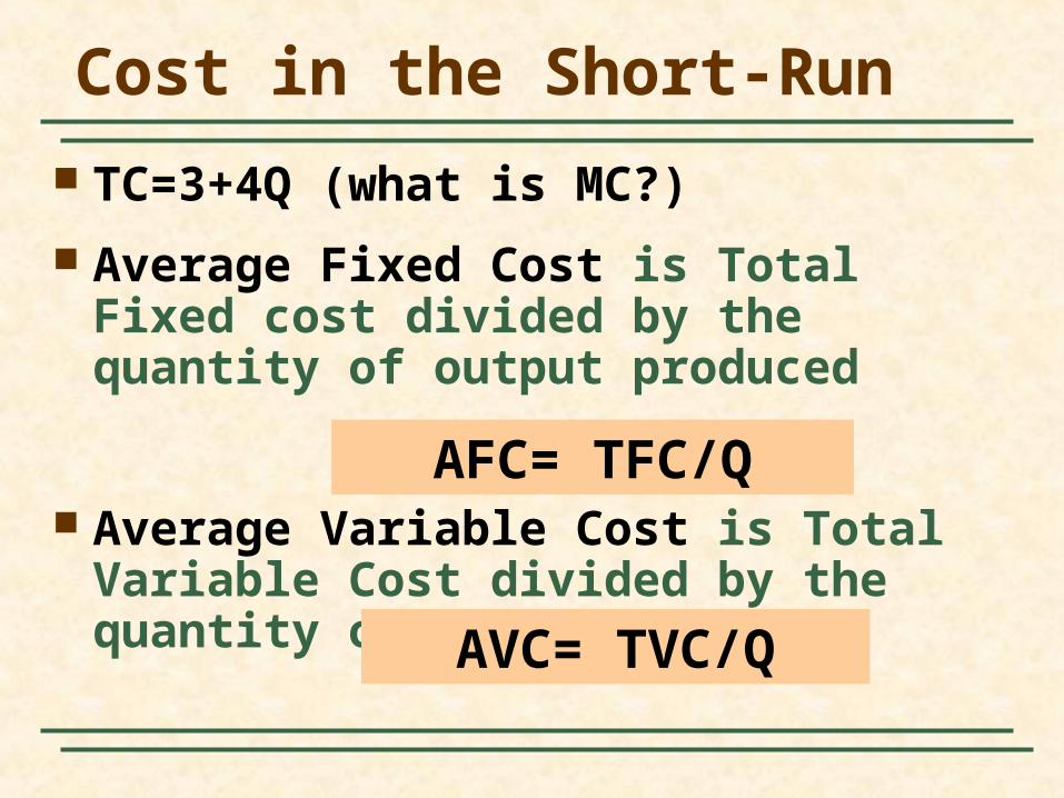
TC=3+4Q (what is MC?)

Average Fixed Cost is Total Fixed cost divided by the quantity of output produced

Average Variable Cost is Total Variable Cost divided by the quantity of output produced

AFC= TFC/Q

AVC= TVC/Q

Cost in the Short Run

Average Cost (AC) is the cost per unit of output, or average fixed cost (AFC) plus average variable cost (AVC).

Q

TVC

Q

TFC ATC

Cost in the Short Run

That is,

Q

TCor AVC AFC ATC

Cost in the Short Run

The Determinants of Short-Run Cost

The relationship between the production function and cost can be exemplified by either increasing marginal returns and decreasing cost or decreasing marginal returns and increasing cost.

Cost in the Short Run

The Determinants of Short-Run Cost Increasing marginal returns and decreasing cost

With increasing marginal returns, output is increasing relative to input and variable cost and total cost will fall relative to output.

Diminishing marginal returns and increasing costWith decreasing marginal returns, output is

decreasing relative to input and variable cost and total cost will rise relative to output.

Cost in the Short Run

Consequently (see the table):MC decreases initially with increasing

marginal returns 0 through 4 units of output

MC increases with decreasing marginal returns (due to law of diminishing marginal returns)

5 through 11 units of output

A Firm’s Short-Run Costs (Rs)

0 50 0 50 --- --- --- ---

1 50 50 100 50 50 50 1002 50 78 128 28 25 39 643 50 98 148 20 16.7 32.7 49.34 50 112 162 14 12.5 28 40.55 50 130 180 18 10 26 366 50 150 200 20 8.3 25 33.37 50 175 225 25 7.1 25 32.18 50 204 254 29 6.3 25.5 31.89 50 242 292 38 5.6 26.9 32.4

10 50 300 350 58 5 30 3511 50 385 435 85 4.5 35 39.5

Rate of Fixed Variable Total Marginal Average Average AverageOutput Cost Cost Cost Cost Fixed Variable Total

(FC) (VC) (TC) (MC) Cost Cost Cost(AFC) (AVC) (ATC)

Cost Curves for a Firm

Output

Cost(Rs.per

year)

100

200

300

400

0 1 2 3 4 5 6 7 8 9 10 11 12 13

VC

Variable costincreases with production and

the rate varies withincreasing &

decreasing returns.

TCTotal cost

is the verticalsum of FC

and VC.

FC50

Fixed cost does notvary with output

Cost Curves for a Firm

Output (units/yr.)

Cost(Rs per

unit)

25

50

75

100

0 1 2 3 4 5 6 7 8 9 10 11

MC

AC

AVC

AFC

A firm’s expansion path shows the minimum cost combinations of labor (L) and capital (K) at each level of output.

Cost in the Long Run

A Firm’s Expansion Path

Labor per year

Capitalper

year

Expansion Path

The expansion path illustratesthe least-cost combinations oflabor and capital that can be used to produce each level of

output in the long-run.

25

50

75

100

150

10050 150 300200

A

Rs2000Isocost Line

200 UnitIsoquant

B

Rs3000 Isocost Line

300 Unit Isoquant

C

A Firm’s Long-Run Total Cost Curve

Output, Units/yr

Costper

Year

Expansion Path

1000

100 300200

2000

3000

D

E

F

Long-Run Average Cost (LAC)

Constant Returns to Scale

If input is doubled, output will double and average cost is constant at all levels of output.

Long-Run Cost Curves and Returns to Scale

Long-Run Average Cost (LAC)

Increasing Returns to Scale

If input is doubled, output will more than double and average cost decreases at all levels of output.

Long-Run Cost Curvesand Returns to Scale

Long-Run Average Cost (LAC)

Decreasing Returns to Scale

If input is doubled, the increase in output is less than twice as large and average cost increases with output.

Long-Run Cost Curvesand Returns to Scale

Long-Run Average Cost (LAC)

In the long-run:

Firms experience increasing and decreasing returns to scale and therefore long-run average cost is “U” shaped.

Long-Run Cost Curvesand Returns to Scale

Long-Run Averageand Marginal Cost

Output

Cost(Rs per unit

of output

LAC

LMC

A

Economies of Scale

Economies of Scale are technological or organisational advantages that accrue to the firm as it increases output in the long run.

Economies of scale reduces long run average costs.(Declining portion of LAC curve)

Economies of ScaleEconomies of Scale occur when increase

in output is greater than the increase in inputs.

Due to advancing technological devt and mass production, there will be reduction in the production costs and prices

Eg: Computer, other consumer electronics etc.

Economies of Scale

Economies of Scale

At higher scales of operation, more specialised and productive machinery can be used.

There are financial reasons for economies of scale

Bulk purchase advantage, bank loans at lower interest rates, decreasing costs in advertisement and promotional activities

Economies of Scale

Economies of scale due to International trade in inputs

Outsourcing accounts for more than one third of total manufacturing costs by Japanses firms, saving them more than 20 % of production costs.

Opening of production facilities abroad

Globalisation and new economies of scale

Diseconomies of Scale

Diseconomies of Scale Increase in output is less than the

increase in inputs.Diseconomies of scale are

organisational disadvantage that the firm encounters as it increases output in the long run.

Diseconomies of scale increase long run average costs (Increasing portion of LAC Curve)

Measuring Economies of Scale by estimating Cost-Output Elasticity

outputin

increase 1% a fromcost in %Δ

elasticityoutput Cost Ec

Measuring Economies of Scale

Cost –Output Elasticity

Cost Elasticity is the percentage change in long run total cost from a 1 per cent change in output

Measuring Economies of Scale

The cost elasticity reflects the presence of either economies of scale or diseconomies of scale

Ec= percentage change in LTC

Percentage change in Q

Measuring Economies of Scale

Ec= LTC . (Q2 +Q1)

Q (LTC2 + LTC1)

Where LTC is Long run Total Cost

Q is output

Measuring Economies of Scale

Measuring Economies of Scale

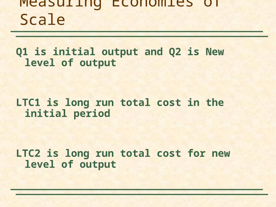
Q1 is initial output and Q2 is New level of output

LTC1 is long run total cost in the initial period

LTC2 is long run total cost for new level of output

Measuring Economies of Scale

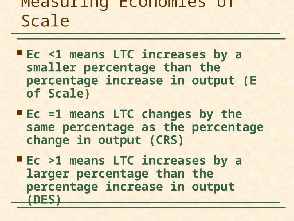
Ec <1 means LTC increases by a smaller percentage than the percentage increase in output (E of Scale)

Ec =1 means LTC changes by the same percentage as the percentage change in output (CRS)

Ec >1 means LTC increases by a larger percentage than the percentage increase in output (DES)

Measuring Economies of Scale

Ec < 1 means Economies of Scale

Ec = 1 means constant returns to scale

Ec > 1 means diseconomies of scale

Economies of Scope

If total cost of production is lower when two products (services) are produced together than when they are produced separately.

Economies of scope occur when the average cost of undertaking two or more activities together is less than the sum of the costs of each activity separately.

Examples:

Automobile company--cars and trucks

University--Teaching and research

A firm that produces a second product in order to use the by-products

What are the advantages of joint production?

Consider an automobile company producing cars and tractors

Economies of Scope

Advantages

1) Both use capital and labor.

2) The firms share management resources.

3) Both use the same labor skills and type of machinery.

Economies of Scope

ObservationsThere is no direct relationship

between economies of scope and economies of scale.

May experience economies of scope and diseconomies of scale

May have economies of scale and not have economies of scope

Economies of Scope

Degree of Economies of Scope measures the savings in cost and can be written:

C(X) is the cost of producing X C(Y) is the cost of producing Y C(X,Y) is the joint cost of producing both

products

),(

),()()C(X SC

YXC

YXCYC

Economies of Scope

Example The ABC Corporation produces 1000 wood

cabinets and 500 wood desks per year, the total cost being $30000. If the firm produced 1000 wood cabinets only, the cost would be $23000. If the firm produced 500 wood desks only, the cost would be $ 11,000.

(a) Calculate the degree of economies of Scope

(b) Why do economies of scope exist?

Example

S= (23000+11000-30000)/30000=0.13

Example

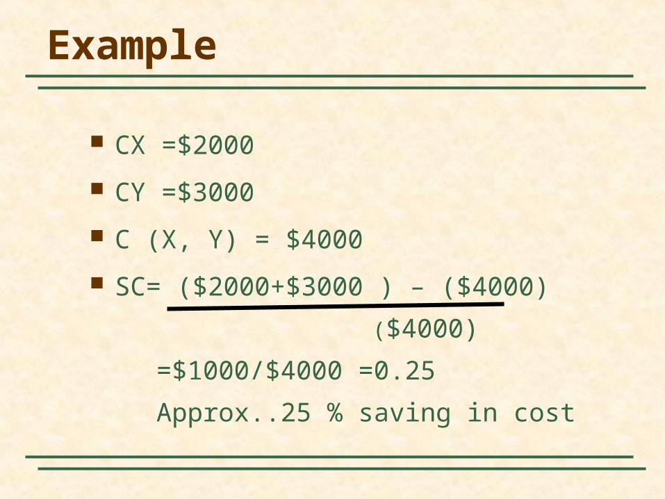
CX =$2000

CY =$3000

C (X, Y) = $4000

SC= ($2000+$3000 ) – ($4000)

($4000)

=$1000/$4000 =0.25

Approx..25 % saving in cost

Interpretation:

If Savings in Cost > 0 -- Economies of scope

If Savings in Cost < 0 -- Diseconomies of scope

Economies of Scope

Estimating and Predicting Cost

Estimates of future costs can be obtained from a cost function, which relates the cost of production to the level of output and other variables that the firm can control.

Suppose we wanted to derive the total cost curve for automobile production.

Either using time series data or cross section data on variables we can estimate cost functions and predict for future.

Difficulties in Measuring Cost

1) Output data may represent an aggregate of different type of products.

2) Cost data may not include opportunity cost.

3) Allocating cost to a particular product may be difficult when there is joint

products.

Estimating and Predicting Cost

Break-even Analysis

Most useful for managerial decision making

A firm is at break even when revenue of the firm is equal to its cost

TR = TC

No profit, No loss

How to calculate Breakeven point Quantity?

Break-even Analysis

Qb = TFC/ (P-AVC)

TFC = Total Fixed Cost

P= Price of product

AVC= Average Variable Cost

Break-even Analysis

Suppose a firm producing a product that has fixed cost per month Rs. 60,000, Average Variable Cost of production is Rs.3.60, Price of Product is Rs.6 per one. What is the breakeven output ?

TFC/ (P- AVC)

60,000/ (6.0 –3.60)

= 25,000 units

Summary

Cost functions relate the cost of production to the level of output of the firm.

Managers, investors, and economists must take into account the opportunity cost associated with the use of the firm’s resources.

Firms are faced with both fixed and variable costs in the short-run.

Summary

When there is a single variable input, as in the short run, the presence of diminishing returns determines the shape of the cost curves.

In the long run, all inputs to the production process are variable. The shape of long run average cost curve is determined by whether firm experiences IRS, CRS or DRS

Summary

The firm’s expansion path describes how its cost-minimizing input choices vary as the scale or output of its operation increases.

A firm enjoys economies of scale when it can double its output at less than twice the cost.

Summary

Economies of scope exist when the joint output of a single firm is greater than the output that could be achieved by two different firms each producing a single output.

Thank you