Run a Better Business

Student NotesS

Cost Volume Profit Analysis

by John Donald, Lecturer, School of Accounting, Economics and Finance, Deakin University, Australia

continued page 11

As mentioned in the last set of Student Notes, the ability to categorise costs as either fixed or variable and to estimate the fixed and variable components of mixed costs, is important because it enables the use of decision making techniques like cost volume profit analysis (CVP analysis). This is essentially a short-term (or tactical) decision tool which shows the effect on profit of changes in costs, prices and sales volume in units. We cannot estimate accurately the impact of these changes unless we know which costs are fixed and which are variable. A manager may want the answers to questions such as ‘what would be the impact on monthly profit of an increase in production and sales of 100 units per month, what increase in sales volume is required to cover the additional fixed costs of our new advertising campaign’ or ‘how many units of product X do we need to make and sell in order for it to be profitable?’ These and other questions can be answered using CVP analysis.

CVP analysis is sometimes called break-even analysis because it allows the user to calculate a break-even point. This is the level of production and sales at which a product or service stops losing money and becomes profitable. At the break-even point profit equals zero. Once we know the break-even point we can assess the financial viability of a new product or analyse our current operating performance.

Assumptions Underlying CVP Analysis

A number of basic assumptions underlie CVP analysis and these need to be kept in mind when assessing its usefulness in a particular decision making situation. The assumptions are:

1. The behaviour of sales revenue and costs is linear throughout the relevant range of activity.

In other words, we assume that selling price per unit, variable cost per unit and the total amount of fixed costs will remain constant during the time period under consideration.

2. The number of units sold is equal to the number of units produced during each period i.e. all the units produced are sold.

3. Variable costs change in total in direct proportion to the level of activity.

4. All costs can be divided into fixed and variable elements.

5. Labour productivity, production technology and market conditions do not change.

6. In multiproduct firms, the sales mix remains constant i.e. the number of units of each product sold will remain a constant percentage of the total number of all the units sold in each period (for all products).

10

11Run a Better Business

N TARGET

CVP analysis is a simplified model of reality, however, in many cases the estimates that it produces are accurate enough to be quite useful. The main danger is using it when a large change in the level of activity will take operations outside the usual or relevant range, so that the CVP assumptions may no longer be valid.

Contribution Income Statement

The starting point for a CVP analysis is the

preparation of a contribution format income statement. This groups together all the variable costs and all the fixed costs for a certain period. Most importantly, it shows the amount of contribution margin as an intermediate figure instead of the gross profit amount shown on a conventional income statement. Contribution margin is the amount of revenue remaining after deducting all variable costs. It can be stated both as a total amount and on a per unit basis as shown in Illustration 1. below.

[CVP analysis is a simplified

model of reality,

however the estimates

that it produces

are accurate enough to be quite useful]

continued page 12

 

Illustration 1. A contribution income statement

12Run a Better Business

Student NotesS

Contribution Margin per Unit

The income statement for the Widmark Clock Company shows that contribution margin per unit ($200) is equal to the selling price per unit ($500) less the variable cost per unit ($300). We will assume that the term cost includes all costs and expenses pertaining to the production and sale of the product. Hence variable costs include variable manufacturing costs plus variable selling and administrative expenses. We can see that for every clock that Widmark makes and sells it will have $200 to cover fixed costs and contribute towards profit. Because total fixed costs are $80, 000 per month, Widmark must generate at least $80, 000 of contribution margin each month before it starts earning any profit. Its monthly sales must exceed 400 clocks ($80 000 ÷ $200). This is Widmark’s break-even point as shown in Illustration 2. below. If Widmark sold 401 clocks in a month its profit before tax for that month would be $200. Once the sales volume of a product passes the break-even point, contribution margin per unit is equal to profit before tax per unit.

Contribution Margin Ratio

The contribution margin ratio (CMR) is the proportion of the selling price per unit represented by contribution margin per unit. For example, if the selling price is $10 per unit and this yields $8.50 in contribution margin, the CMR is 85 per cent or 0.85. Alternatively, the CMR is the proportion of total sales revenue represented by the total contribution margin amount. For the Widmark Clock Company the CMR is $200 ÷ $500 or 40 per cent. Out of each sales dollar 40 cents is available to apply to fixed costs and to contribute to profit. If Widmark’s sales revenue increased by $20, 000 from $200, 000 in August to $220, 000 in September its profit before tax would increase from zero to $8 000 ($20 000 x 40 per cent).

Using the CMR enables managers to quickly determine the effect on profit from any planned change in sales provided that the change does not take the level of activity outside the relevant range. If this occurs, total fixed costs and/or variable cost per unit may change. The relevant range is an important limitation on CVP analysis. If we were considering an infinitely large range of output and sales, starting from zero, all costs would tend to be variable. The assumptions that total fixed costs will remain constant and that variable cost per unit does not change are only valid within the normal or relevant range.

Note that the contribution margin ratio plus the variable cost ratio (total variable costs ÷ sales revenue) equals 100 per cent i.e. CMR + VCR = 100 per cent (or 1.0)

Illustration 2. A contribution income statement at the break-even point

continued page 13

 

[Using the CMR enables managers to quickly determine the effect on profit from any planned change in sales]

13Run a Better Business

N TARGET

Calculating the Break-Even Point

The break-even point can be calculated in three ways:

1. The graphical method

2. The equation method

3. The contribution margin method

1. The Graphical Method

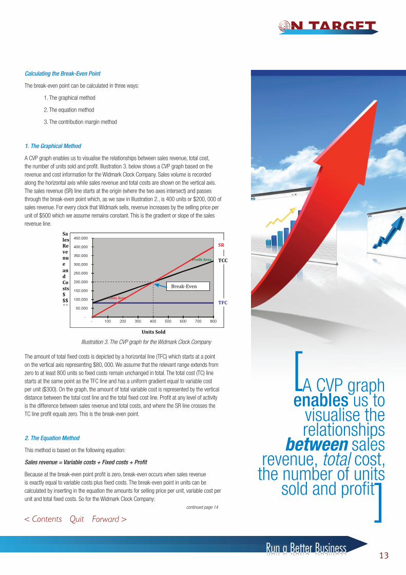
A CVP graph enables us to visualise the relationships between sales revenue, total cost, the number of units sold and profit. Illustration 3. below shows a CVP graph based on the revenue and cost information for the Widmark Clock Company. Sales volume is recorded along the horizontal axis while sales revenue and total costs are shown on the vertical axis. The sales revenue (SR) line starts at the origin (where the two axes intersect) and passes through the break-even point which, as we saw in Illustration 2., is 400 units or $200, 000 of sales revenue. For every clock that Widmark sells, revenue increases by the selling price per unit of $500 which we assume remains constant. This is the gradient or slope of the sales revenue line.

The amount of total fixed costs is depicted by a horizontal line (TFC) which starts at a point on the vertical axis representing $80, 000. We assume that the relevant range extends from zero to at least 800 units so fixed costs remain unchanged in total. The total cost (TC) line starts at the same point as the TFC line and has a uniform gradient equal to variable cost per unit ($300). On the graph, the amount of total variable cost is represented by the vertical distance between the total cost line and the total fixed cost line. Profit at any level of activity is the difference between sales revenue and total costs, and where the SR line crosses the TC line profit equals zero. This is the break-even point.

2. The Equation Method

This method is based on the following equation:

Sales revenue = Variable costs + Fixed costs + Profit

Because at the break-even point profit is zero, break-even occurs when sales revenue is exactly equal to variable costs plus fixed costs. The break-even point in units can be calculated by inserting in the equation the amounts for selling price per unit, variable cost per unit and total fixed costs. So for the Widmark Clock Company:

Illustration 3. The CVP graph for the Widmark Clock Company

continued page 14

[A CVP graph enables us to

visualise the relationships

between sales revenue, total cost, the number of units

sold and profit]

 

 Break-­‐Even  Point  

Profit  Area  

       Loss  Area  

                     Units  Sold  

Sales  Revenue  and  Costs  $  $$$$RRevenue  $Revenue  Revenue  

SR  

TCC  

TFC  

14Run a Better Business

Student NotesS

Sales revenue = Variable costs + Fixed costs + Profit

$500Q = $300Q + $80,000 + $0

Where:

Q = Number of clocks sold

$500 = Selling price per unit

$300 = Variable cost per unit

$80,000 = Total fixed costs

Now solve for the value of Q:

$500Q = $300Q + $80,000 + $0

$200Q = $80,000

Q = $80,000 ÷ $200

Q = 400 clocks

This is the break-even point in terms of units sold. To find the sales revenue needed to break-even, we multiply the number of units sold at the break-even point by the selling price per unit:

400 x $500 = $200, 000 (break-even sales revenue)

3. The Contribution Margin Method

The third method of calculating the break-even point is derived from the equation method described above. When we solved for the value of Q, the last step involved dividing total fixed costs by the contribution margin of $200 per unit to give break-even units (Q = 400). This simple calculation can be expressed thus:

Break-even point in units sold = Total fixed costs

Contribution margin per unit

400 = $80,000 ÷ $200

To calculate the amount of break-even sales revenue we use the contribution margin ratio instead of contribution margin per unit:

Break-even point in dollars of sales revenue = Total fixed costs

Contribution margin ratio

$200, 000 = $80,000 ÷ 0.4

The contribution margin method can be extended to give the number of sales units or sales dollars required to reach a certain target profit figure simply by adding the target profit to the total fixed cost amount in the break-even formula. Note that the target profit figure we must use is the profit required before tax has been deducted. If you are given a target profit figure after tax, dividing it by (1 – the tax rate) will convert it into the larger before tax amount:

Target profit before tax = (target profit after tax) ÷ (1 – t)

where t denotes the income tax rate.

CVP Analysis with Multiple Products

So far we have considered situations involving single products. However, the reality is that there are very few single product organisations. CVP analysis can be adapted for situations where there is more than one product being made and sold. For example, assume that the Contex Calculator Company produces two types of calculator: Model A and Model B. Their details are as follows:

Model A Model B

Selling Price Per Unit $30 $50

Variable Cost per Unit 15 20

Contribution Margin Per Unit $15 $30

Sales Mix 2 1

Contex typically sells two Model A calculators for each Model B that is sold. The sales mix is, therefore, two to one. Assume that Contex’s total fixed costs are $100, 000.

We can now calculate the weighted average contribution margin (WACM) per unit using the sales mix numbers as weights. Since two Model As are sold for each Model B, the contribution margin of A is multiplied by 2, and the contribution margin of B is multiplied by 1. The sum of the answers is then divided by 3 (the sum of the weights) to give the weighted average contribution margin per unit of $20.

WACM per unit = ($15 x 2) + ($30 x 1)

3

= $20

The weighted average contribution margin per unit can now be used to calculate the break-even point in units:

Break-even sales in units = Total fixed costs

WACM per unit

= $100, 000 ÷ $20

= 5, 000

These 5, 000 units would consist of 3, 333 units of Model A (two-thirds of 5, 000) and 1, 667 units of Model B (one-third of 5, 000).

Check: TCM = (3, 333 x $15) + (1, 667 x $30) = $100, 005 = TFC ($5 rounding error)

Although the method we have just used is appropriate for situations where the sales mix is constant, in reality a constant sales mix is very rare. If a firm’s sales mix does vary over time, one of the main assumptions underlying CVP analysis becomes invalid and the results it produces become less reliable.