Counting, Generating, and Solving Sudoku

Mathias Weller

April 21, 2008

Abstract

In this work, we give an overview of the research done so far on thetopic of Sudoku grid enumeration, solving, and generating Sudoku puz-zles. We examine possible extensions and generalizations of previous workon solving and generating Sudoku puzzles focusing mainly on rulebasedsolvers. A possible way to influence the difficulty of a generated Sudokupuzzle is described and we introduce new deduction rules for solving apuzzle based on the rules described by David Eppstein in his paper “Non-repetitive Paths and Cycles in Graphs with Application to Sudoku”. Wethen generalize these new rules further leading to an efficient constraintpropagation algorithm that is able to solve puzzles that could not besolved by applying only Eppstein’s deduction rules. The implementationof this strategy and how it may be used to implement the special casesis explained, followed by a practical evaluation of the solving power of allpresented solvers.

1

Contents

1 Introduction 31.1 The Sudoku Game . . . . . . . . . . . . . . . . . . . . . . . . . . 31.2 Sudoku Variants . . . . . . . . . . . . . . . . . . . . . . . . . . . 6

2 Prior Work 72.1 Counting Sudoku Grids . . . . . . . . . . . . . . . . . . . . . . . 92.2 Complexity . . . . . . . . . . . . . . . . . . . . . . . . . . . . . . 11

2.2.1 Short Introduction to NP-completeness . . . . . . . . . . 112.2.2 Sudoku Decision Problem . . . . . . . . . . . . . . . . . . 122.2.3 Complexity of the Sudoku Decision Problem . . . . . . . 12

2.3 Generating Sudoku Puzzles . . . . . . . . . . . . . . . . . . . . . 132.3.1 Incremental Generation . . . . . . . . . . . . . . . . . . . 132.3.2 Decremental Generation . . . . . . . . . . . . . . . . . . . 14

2.4 Judging the Difficulty of Generated Sudoku Puzzles . . . . . . . 142.5 Finding Solutions to Sudoku Puzzles . . . . . . . . . . . . . . . . 15

2.5.1 Solving Sudoku Puzzles via Backtracking . . . . . . . . . 152.5.2 Solving Sudoku Puzzles via Constraint Programming . . . 152.5.3 Solving Sudoku Puzzles via Logic Deduction . . . . . . . 16

2.6 Graph Coloring . . . . . . . . . . . . . . . . . . . . . . . . . . . . 18

3 Generalization and Contribution 183.1 Counting Sudoku . . . . . . . . . . . . . . . . . . . . . . . . . . . 193.2 Generating Sudoku Puzzles . . . . . . . . . . . . . . . . . . . . . 20

3.2.1 Finding a Full Sudoku Grid . . . . . . . . . . . . . . . . . 203.2.2 Deletion Witnesses . . . . . . . . . . . . . . . . . . . . . . 21

3.3 Judging the Difficulty of Generated Sudoku Puzzles . . . . . . . 213.4 Finding Solutions to Sudoku Puzzles . . . . . . . . . . . . . . . . 21

3.4.1 Extension of Bilocation and Bivalue . . . . . . . . . . . . 223.4.2 Group-Modified Rules . . . . . . . . . . . . . . . . . . . . 253.4.3 Limited Constraint Propagation . . . . . . . . . . . . . . 26

4 Experimental Results 31

5 Outlook and Future Work 32

2

1 Introduction

Sudoku (or “Number place”, as it is called in the US) is a well-known logicpuzzle popular for its appearance in newspapers and magazines. Its popular-ity is expressed in examples like a Boston Japanese restaurant that hands out$10 gift certificates to patrons who can finish a Sudoku puzzle before their Sushiis served. There are official tournaments in Europe and the US with the possi-bility to win monetary prizes [Sem05]. Solving a Sudoku puzzle is usually verysatisfactory for the puzzler, or, to quote Henry Dudeney, “A good puzzle, likevirtue, is its own reward” [Dud02]. Sudoku is a derivative of Latin Square, apuzzle first described by Leonhard Euler in 1783. The Sudoku puzzle was firstcreated for Dell Magazines by Howard Garnes, an architect from Indianapolisand introduced to the US public in 1979. It was not until seven years laterthat Sudoku was successful in Japan, where it was first published by the Nikolicompany under its current name, which is Japanese for “single number”. Atthe beginning of the 21st century, the puzzle spread all over the world. Thisinternational success partially relies on using numbers instead of letters or words[Sem05]. When solving Sudoku puzzles, one naturally stumbles upon a varietyof questions: Does my puzzle have a solution? If so, is it the only one for mypuzzle? If not, how many solutions are there and is there a systematic way of de-termining all solutions? Does the puzzle become harder if there were less hints?What is the minimum number of hints in order to assure a unique solution? Inthis article, we will consider some of these and other questions.

1.1 The Sudoku Game

Sudoku is a puzzle game played on a grid that consists of 9 × 9 cells eachbelonging to three groups: one of nine rows, one of nine columns and one ofnine blocks (sometimes called boxes or subsquares). Three blocks in a row arecalled a band, three vertically stacked blocks are called a stack, a chute is eithera band or a stack (see Figure 1). A Sudoku grid is full, if each group containsthe numerals from 1 to 9 exactly once. Figure 1 shows a full Sudoku grid. ASudoku puzzle is a Sudoku grid that is partially filled, meaning that a set offixed cells (cells whose numerals are given, i.e. that cannot be chosen by thesolver), also called hints or clues is provided by a puzzle master, whereas theother cells are blank. Figure 2 shows a possible Sudoku puzzle for the grid inFigure 1. The objective of the puzzle game is to fill the Sudoku grid by assigninga numeral to each blank cell in such a way that each numeral is unique in eachof its three groups. A solution to a Sudoku puzzle is a full Sudoku grid that isconsistent with the puzzle, meaning that all hints of the puzzle appear in the fullgrid as well. Figure 1 is a solution to the puzzle in Figure 2. A Sudoku grid iscalled proper or unisolvent if it has only one solution, ambiguous if it has morethan one solution and invalid if it has no solution at all, due to contradictinghints. Most daily newspaper Sudoku puzzles provide about 28 or 30 clues,but for the difficulty of the puzzle, the number of hints matters less than thecomplexity of the logical leaps required to assign numerals to the blank cells

3

1 3 8 2 7 6 5 4 92 7 5 4 1 9 8 6 36 4 9 5 8 3 1 7 25 8 3 1 6 7 2 9 49 1 6 3 4 2 7 5 87 2 4 9 5 8 3 1 63 5 2 7 9 4 6 8 14 6 1 8 3 5 9 2 78 9 7 6 2 1 4 3 5

1 3 8 2 7 6 5 4 92 7 5 4 1 9 8 6 36 4 9 5 8 3 1 7 25 8 3 1 6 7 2 9 49 1 6 3 4 2 7 5 87 2 4 9 5 8 3 1 63 5 2 7 9 4 6 8 14 6 1 8 3 5 9 2 78 9 7 6 2 1 4 3 5

Figure 1: A full Sudoku grid. On the right, the first band and the second stackare marked.

1 7 92 5 6

3 15 8 1 6

6 75 8 1 6

2 76 9 7

8 2 5

Figure 2: A proper Sudoku puzzle.

4

[Sem05]. As opposed to the difficulty, the number of clues plays a crucial role indetermining the properness of a puzzle. So far, no proper 9× 9 Sudoku puzzleswith less than 17 hints is known, whereas there are several proper puzzles withexactly 17 hints. The minimal number of hints necessary for an n×n puzzle tohave a unique solution is yet unknown [HM07], although a lower bound of n−1is easy to prove: if a puzzle had only n − 2 hints, then there are two numeralsthat are not specified by the puzzle. These two numerals may be exchangedthroughout the solution to the puzzle in order to obtain another solution for itand thus, the puzzle cannot be proper (see also Section 2.6 on page 18).

In order to do complexity analysis for solving Sudoku puzzles, we parametrizethem. In this case, the size of each group (meaning the number of differentnumerals) (n = 9), the order of the Sudoku grid, meaning the length of aside of the blocks (m =

√n = 3), or the number of cells in the Sudoku grid

(h = n2 = 81) may be used. Since they are all polynomial in one another,an efficient algorithm with regard to any of these parameters is efficient withregard to all of them, hence efficiency is invariant under choosing one of thementioned parameters. For reasons of compatibility with other papers, n willrefer to the number of different numerals in the following part of the article,if not explicitly stated otherwise. Though it is common to use numerals to fillthe Sudoku grid, letters, pictures or any kind of items dividable into at leastn disjoint equivalence classes is suitable as well.

Sudoku is closely related to the Latin Square problem: given an n ×n square of cells and a set of fixed cells, find a completely filled n× n grid thatis a superset of the fixed cells such that each item is unique for its column androw while still using only n different types of items. Figure 3 shows an exampleof a Latin Square puzzle and its solution.

6 4 2 13 9 4 84 6 3 75 2 8 9

8 1 3 21 7 3

2 8 6 1 74 9 5 1 8

3

6 8 4 3 7 2 1 5 91 3 6 9 4 5 7 2 89 4 2 6 1 8 3 7 57 5 3 2 8 4 9 6 18 6 7 1 5 3 4 9 25 9 1 8 2 7 6 3 43 2 8 4 9 6 5 1 74 7 9 5 3 1 2 8 62 1 5 7 6 9 8 4 3

Figure 3: A 9× 9 Latin Square puzzle and its solution.

5

1 3 7 46 2 3

7 84 3 7

2 7 47 8

3 8 18 5 3 6

Figure 4: An 8× 8 Sudoku puzzle with 2× 4 groups.

Figure 5: The 12 pentomino groups.

1.2 Sudoku Variants

Although this article is mainly about plain Sudoku as described above, thisshort introduction to Sudoku variants may be of interest for the reader.

As already mentioned, a Sudoku grid may have any dimension n, although9×9 puzzles are by far the most common. There are also puzzles that do not havethe same number of stacks and bands. An example is the 8× 8 Sudoku puzzleshown in Figure 4. The groups may be irregular, which allows for 5×5 grids withpentomino groups (groups of irregular shape that contain exactly five cells, seeFigure 5). This type of puzzle is also known as “Logi-5”. Apart from geometricdifferences, there are several Sudoku variants that impose new rules or modifythe existing rules of the puzzle: The Sudoku X variant enforces the numeralsin the cells on the diagonals to be unique for each diagonal (see Figure 6)[Mon05]. The Hypersudoku variant, also called Windocu consists of a normalSudoku grid that is supplemented with additional regions that have to containeach numeral exactly once. These regions overlap the blocks, thereby givingadditional information (see Figure 6). The Samurai Sudoku variant consists offive 9 × 9 Sudoku puzzles arranged in a quincunx1 such that the grid in the

1A quincunx is a formation of five entities similar to a cross. For example, the five dots ona side of a dice form a quincunx.

6

5 4 6 1 2 7 8 3 98 9 7 4 5 3 2 1 62 3 1 9 6 8 7 5 41 7 8 6 4 5 3 9 26 2 9 7 3 1 5 4 83 5 4 8 9 2 6 7 17 1 2 5 8 9 4 6 39 6 3 2 7 4 1 8 54 8 5 3 1 6 9 2 7

Figure 6: Left: A 9× 9 Sudoku X grid. Right: A 9× 9 Hypersudoku grid.

middle is being overlapped by the other four grids in its four corners, such thatthe middle grid shares one block with each of the other grids while the outergrids are disjoint (see Figure 7) [Tel06]. The circular Sudoku variant employs acircular formation of cells that is divided into segments and rings. Each cell hasto be assigned a numeral such that each ring and each pair of neighboring sectorscontain each numeral exactly once (see Figure 8) [PMH06]. A variant combiningthe idea of the Rubik’s cube with Sudoku puzzles is the Sudokucube, a 3× 3× 3cube that can be solved by turning plains of subcubes in such a way that eachside becomes a valid Sudoku grid. Hence the cube contains the numbers 1 to 9exactly 6 times each. Variants that use letters instead of numerals may enforcethe formation of a valid word at some place in the grid. For almost every Sudokuvariant, there is another variant with the nonconsecutive property, meaning thatno two neighboring cells may be assigned consecutive numerals. Other variantsmay modify the way in which hints are given, for example the 2005 U.S. PuzzleChampionship featured a puzzle that contained ranges of numerals as hints.

2 Prior Work

In this chapter, publications about Sudoku puzzles are being introduced: Fora start, we will consider the problem of counting possible Sudoku grids in Sec-tion 2.1. A general complexity consideration in Section 2.2 will introduce tothe topic of generating (Section 2.3) and solving (Section 2.5) Sudoku puzzles.In Section 2.4, the problem of judging the difficulty of a generated puzzle willbe addressed. We will show parallels to the Graph-n-Coloring problem inSection 2.6. Chapter 3 will introduce thoughts and ideas developed from theapproaches of Chapter 2 and finally, results of applying some of these ideas aregiven in Chapter 4.

7

9 3 7 1 8 6 4 2 5 1 6 4 3 9 5 2 7 81 2 4 5 7 9 3 8 6 8 2 3 1 7 4 5 6 96 5 8 2 3 4 7 9 1 9 5 7 2 8 6 4 1 32 6 1 4 5 7 9 3 8 4 8 5 7 6 9 1 3 28 7 5 3 9 2 1 6 4 7 9 2 5 3 1 6 8 44 9 3 8 6 1 5 7 2 3 1 6 8 4 2 7 9 55 8 2 7 1 3 6 4 9 7 1 5 2 3 8 4 1 7 9 5 63 1 6 9 4 8 2 5 7 8 3 9 6 4 1 9 5 3 8 2 77 4 9 6 2 5 8 1 3 2 6 4 5 7 9 6 2 8 3 4 1

3 6 4 1 9 2 8 5 71 7 8 5 4 6 9 2 35 9 2 3 8 7 4 1 6

9 2 7 3 5 6 4 8 1 9 5 3 7 6 2 5 1 3 4 9 85 3 8 4 7 1 9 2 6 4 7 1 3 8 5 4 6 9 2 1 74 6 1 9 2 8 7 3 5 6 2 8 1 9 4 8 7 2 6 3 56 7 3 5 8 9 1 4 2 5 3 7 2 9 4 1 8 62 8 4 1 6 3 5 7 9 4 1 6 3 8 7 9 5 21 5 9 7 4 2 8 6 3 8 2 9 6 5 1 7 4 37 1 5 2 3 4 6 9 8 6 4 3 1 2 8 5 7 93 9 6 8 1 7 2 5 4 9 5 8 7 4 6 3 2 18 4 2 6 9 5 3 1 7 2 7 1 9 3 5 8 6 4

Figure 7: A 9× 9 Samurai Sudoku grid.

Figure 8: A circular Sudoku puzzle with n = 8.

8

2.1 Counting Sudoku Grids

This section is a short summary of what was done so far on the topic of de-termining the number of full Sudoku grids of specific dimensions. For a moredetailed view, please refer to the literature given in the section.

First of all, we are interested in the number of different full Sudoku grids ofa certain order. To calculate this number, we first need a definition of differenceregarding Sudoku grids. Therefore, an equality relation is to be provided thatrelates equal Sudoku grids. Hence two grids that are not related are considereddifferent. For the following lemmas, two Sudoku grids are considered equal ifevery cell of a grid contains the same numeral as the cell at the same positionin the other grid. This equality relation will be referred to as E.

Lemma 2.1 ([HM07]) There are N4×4 = 288 valid full 4× 4 Sudoku grids.

Lemma 2.2 ([FJ06]) There are

N9×9 = 6, 670, 903, 752, 021, 072, 936, 960

valid full 9× 9 Sudoku grids.

Remark The lemmas were proved using a combination of symmetry consider-ation and brute force calculation, which did not allow for the calculation of theexact number of valid 16× 16 Sudoku grids yet, so this is an open problem.

This result may satisfy for the time being, but the fact that in order to calculatethese numbers a Sudoku grid and the version of the grid that is simply rotated by90 are considered different may be disturbing. Hence another equality relationis presented:

Definition Let S denominate the set of all full Sudoku grids of a certain order.A transformation t : S → S is called validity-preserving. Let T be a set ofvalidity-preserving transformations. We define the equality relation ET ⊆ S×Swith

(s1, s2) ∈ ET ⇔ ∃k ∈ N ∃t1, . . . , tk ∈ T ((t1 t2 . . . tk)(s1), s2) ∈ E.

Remark The relation ET relates two grids iff one can be transformed into theother by using only transformations in T . Note that being validity-preserving isinvariant with respect to composition, thus t1t2 . . .tk is a validity-preservingtransformation but is not necessarily in T .

So far, a number of transformations that preserve the validity of a Sudoku gridare known. For example, a Sudoku grid may be rotated by a multiple of 90

without affecting its validity. Furthermore, it is possible to permute the numer-als throughout the entire grid without changing the validity of the grid becausegenerally the items in a Sudoku grid are not ordered. More transformations willbe mentioned later in this section and additional possibilities will be discussedin Section 3.2.1.

9

Definition Let T1 be the set that consists of the following validity-preservingtransformations:

• Permuting numerals

• Permuting rows in the same band

• Permuting bands

• Transposing the grid (That is, mirroring the grid by the main diagonal)

The equality relation E′ := ET1 is being referred to when speaking of essentiallydifferent Sudoku grids. For irregular puzzle sizes, the transposition is not va-lidity preserving. The following transformations are referred to when speakingof essentially different irregular Sudoku grids:

• Permuting numerals

• Permuting rows in the same band

• Permuting bands

• Permuting columns in the same stack

• Permuting stacks

Lemma 2.3 ([HM07]) There are N ′4×4 = 2 essentially different 4×4 Sudokugrids (see Figure 9).

1 2 3 4 1 2 3 43 4 1 2 3 4 2 12 1 4 3 2 1 4 34 3 2 1 4 3 1 2

Figure 9: Representatives of the only two equivalence classes of 4 × 4 Sudokugrids with respect to essentially different Sudoku grids.

Lemma 2.4 ([RJ06a]) There are N ′9×9 = 5, 472, 730, 538 essentially different9× 9 Sudoku grids.

Other Sudoku variants were analyzed as well. Applying the transformationslisted in Definition 2.1 to different grid sizes results in different numbers of fullgrids. An overview about these results is given in Table 1.

10

Grid type Block types Number of essentially different Sudoku grids

4× 4 2× 2 2 (See Lemma 2.3)6× 6 2× 3 49 [RJ06b]8× 8 2× 4 1, 673, 187 [Rus06]

10× 10 2× 5 4, 743, 933, 602, 050, 718 [Pet06]9× 9 3× 3 5, 472, 730, 538 (See Lemma 2.4)

Table 1: Number of different Sudoku grids with respect to E′ for differentpuzzle sizes. Note that different transformations apply for irregular Sudokupuzzle sizes.

2.2 Complexity

From the point of view of a student of theoretical computer science, a veryimportant consideration is the complexity analysis of a problem. In this section,we will discuss the decision variant of the Sudoku problem. This will be definedin Section 2.2.2, after a short introduction to NP-completeness.

2.2.1 Short Introduction to NP-completeness

This section will provide a brief overview over the topic of NP-completeness.First of all, it is important to know some terms: In computer science, an algo-rithm is called deterministic if each step is determined only by prior steps andthe input data. A deterministic algorithm is called efficient if its running timeis bounded by a polynomial in the size of the input data. The set of problemsthat are solvable efficiently is denominated by P, while NP denominates the setof problems whose solutions are efficiently verifiable. Let A and B be problemsin NP, then a function f is called a reduction from A to B if for any input d,d ∈ A ⇔ f(d) ∈ B and the computation of f(d) is deterministic and efficient.So the question whether d ∈ A can be answered by applying the reduction f tod and testing whether f(d) ∈ B. If such a function exists for two problems Aand B, A is called reducible to B. Note that if f(d) ∈ B can be determined effi-ciently, so can d ∈ A. Also note that the binary reducible-relation is transitive,meaning that if A is reducible to B and B is reducible to C, A is also reducibleto C. A problem Q in NP is called NP-complete, if all problems in NP can bereduced to it. Hence, if Q was solvable efficiently, all problems in NP would be.For example, the SAT Problem, which is to tell whether a given Boolean for-mula in conjunctive normal form has a satisfying assignment, in other words, ifthe formula can evaluate to true, is NP-complete. It is yet unknown if efficientlyfinding solutions to the problems in NP is possible. This is called the P vs. NPProblem.

11

2.2.2 Sudoku Decision Problem

We refer to “the Sudoku problem” as the problem of finding a solution to agiven Sudoku puzzle. Much like SAT, where the decision problem is to findwhether a satisfying assignment of all variables of a given formula exists, thedecision problem for Sudoku is to find whether a solution to a given Sudokupuzzle exists. Note that it does not matter if the solution is ambiguous or not,the uniqueness of a solution is not of interest. The decision variant of the LatinSquare problem is defined analogously.

2.2.3 Complexity of the Sudoku Decision Problem

The Sudoku decision problem is in NP. Obviously, the size of an n×n Sudokugrid is polynomial in n and thus a given solution to the grid can be verifiedefficiently. It has been shown that the decision problem of Sudoku is NP-complete by reducing Latin Square, which is known to be NP-complete, toSudoku [YS03]. In the following, a sketch of the proof will be presented: Tosolve an n × n Latin Square, we construct a k × k Sudoku grid with k = n2

as follows: let S(i, j) denote the numeral in the cell of the Sudoku grid whosecolumn is i and whose row is j and let L(r, s) denote the cell of the Latin Squarewhose column is r and whose row is s. The Sudoku grid is then constructedrespecting the equation

S(i, j) =

r(L(i− 1, (j − 1)/n)) , if stack((i, j)) = rowband((i, j)) = 1,trn((i, j)) , otherwise

withtrn(x) = (colstack(x) · n + stack(x) + row(x)) mod n2 + 1

where rowband(x) stands for the number of the row in the band of cell x, andcolstack(x) stands for the number of the column in the stack of cell x. Thefunctions stack(x) and row(x) stand for the stack and the row of x respectively.This leads to

S(i, j) =

r(L(i− 1, j−1

n )) , if⌊

i−1n

⌋= (j − 1) mod n = 0,

trn((i, j)) , otherwise.

with r being a bijection that maps the n numerals of the Latin Square to n ofthe k numerals of the Sudoku:

r(x) = (x− 1) · n + 1,

and

trn(x) = (((i− 1) mod n) · n +⌊

i− 1n

⌋+ j − 1) mod n2 + 1.

This construction enforces the assignment of all numerals d with

∃x ∈ 0, . . . , n : d = r(x)

12

22

1

4 2 5 8 3 6 92 5 8 3 6 9 4 7 13 6 9 4 7 1 5 8 2

4 5 8 2 6 9 35 8 2 6 9 3 7 1 46 9 3 7 1 4 8 2 51 8 2 5 9 3 6

8 2 5 9 3 6 1 4 79 3 6 1 4 7 2 5 8

Figure 10: An example for the reduction from Latin Square to Sudoku.

to the cells with ⌊i− 1

n

⌋= (j − 1) mod n = 0

but does not enforce any ordering on them other than the Latin Square rules forthe resulting grid to comply with the Sudoku rules. Figure 10 shows an examplefor the reduction of a 3 × 3 Latin Square: together, the gray cells make up asolution to the given Latin Square. The numerals 1, 4 and 7 in the gray cells ofthe Sudoku grid are translated to the numerals 1,2 and 3 in the Latin Square.

2.3 Generating Sudoku Puzzles

Generating a Sudoku puzzle is the task of choosing a subset of cells of theSudoku grid to contain hints to enable the solver to calculate a solution forthe puzzle. To be satisfactory for human solvers, the solution implied by thehints should be unique, so it is desirable to generate proper puzzles. Basically,there are two different methods to create a proper Sudoku puzzle: Incrementalgeneration, which assigns numerals to one cell after another until sufficient hintsare given for the puzzle to have a unique solution. Decremental generationremoves numerals from the cells of a full Sudoku grid for as long as desired orpossible in order for the solution to stay unique.

2.3.1 Incremental Generation

Several Sudoku programmer forums advice to implement Sudoku generatorsthat (randomly) pick cells and assign a (random) non-conflicting numeral tothem until an automated solver can solve it. The disadvantage of this methodis that determining if a numeral contradicts another in a partially filled Sudokugrid in general requires a solver. When assigning a random numeral to a ran-dom cell, the puzzle may become invalid so the generator must either utilizebacktracking to find another cell or numeral, or discard the whole puzzle andstart over when a puzzle becomes invalid.

13

1 2 3 4 5 6 7 8 94 5 6 7 8 9 1 2 37 8 9 1 2 3 4 5 62 3 4 5 6 7 8 9 15 6 7 8 9 1 2 3 48 9 1 2 3 4 5 6 73 4 5 6 7 8 9 1 26 7 8 9 1 2 3 4 59 1 2 3 4 5 6 7 8

Figure 11: Trivial Sudoku grid generated by S(x, y) = ((bx/mc+m·(x mod m)+y) mod n) + 1, where x is the number of the row of the cell starting with 0 andy is the number of its column starting with 0, n is the number of numerals andm =

√n is the order of the Sudoku grid.

2.3.2 Decremental Generation

To generate a Sudoku puzzle decrementally, we have to create a completelyfilled grid first. There are multiple methods for how this can be achieved: Forinstance, we could just take an existing Sudoku grid or generate a trivial Sudokugrid by employing a mathematical formula (see Figure 11). The transformationof an existing grid using validity-preserving transformations will also yield a newSudoku grid. We can also employ an algorithm for incremental generation ofSudoku puzzles and apply a solver to it. This last method may seem intricatebut may be of interest for complexity analysis. After generating a full Sudokugrid, the numerals from this grid are being removed for as long as possible forthe solution to stay unique. Therein lies the problem of indirect generation ofSudoku puzzles, because determining if a Sudoku grid is proper is not trivialand usually requires a solver. If the removal of a numeral causes the puzzle tonot be proper anymore, backtracking is used or the puzzle is discarded.

2.4 Judging the Difficulty of Generated Sudoku Puzzles

With the generation of a Sudoku puzzle comes the task to judge its difficulty. Tothe best of our knowledge, all Sudoku puzzle generators determine the difficultyof a puzzle after its generation, which has the disadvantage that one cannotchoose the difficulty of the puzzle to be generated. In order to get a puzzle ofdesired difficulty, the generator may have to be run multiple times. Eppstein’sgenerator judges a puzzle by the logic rules needed to solve it. Each rule isassigned a value and the difficulty value of the puzzle equals the maximumdifficulty value of all rules needed to solve it, where the solver only applies adifficult rule if all simpler rules have been exhausted [Epp05b]. This means thatif we were to generate a Sudoku puzzle of a certain difficulty, we would need an

14

automated solver.

2.5 Finding Solutions to Sudoku Puzzles

Finding solutions to Sudoku puzzles is easily done by a simple backtrackingalgorithm explained in Section 2.5.1. However, there are two main reasons whythis is not desirable: Backtracking in general takes too much time and it is notfitting to judge the difficulty of a Sudoku puzzle. For the purpose of simulating ahuman solver and thus evaluating the difficulty of a Sudoku puzzle in context ofhuman strategies, solving it with a set of deduction-rules is of great interest. Forthese reasons this article is focused on (efficient) non-backtracking algorithmsfor solving Sudoku puzzles and just briefly introduces other options.

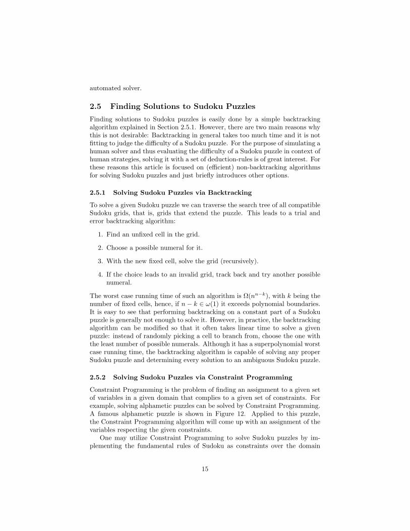
2.5.1 Solving Sudoku Puzzles via Backtracking

To solve a given Sudoku puzzle we can traverse the search tree of all compatibleSudoku grids, that is, grids that extend the puzzle. This leads to a trial anderror backtracking algorithm:

1. Find an unfixed cell in the grid.

2. Choose a possible numeral for it.

3. With the new fixed cell, solve the grid (recursively).

4. If the choice leads to an invalid grid, track back and try another possiblenumeral.

The worst case running time of such an algorithm is Ω(nn−k), with k being thenumber of fixed cells, hence, if n− k ∈ ω(1) it exceeds polynomial boundaries.It is easy to see that performing backtracking on a constant part of a Sudokupuzzle is generally not enough to solve it. However, in practice, the backtrackingalgorithm can be modified so that it often takes linear time to solve a givenpuzzle: instead of randomly picking a cell to branch from, choose the one withthe least number of possible numerals. Although it has a superpolynomial worstcase running time, the backtracking algorithm is capable of solving any properSudoku puzzle and determining every solution to an ambiguous Sudoku puzzle.

2.5.2 Solving Sudoku Puzzles via Constraint Programming

Constraint Programming is the problem of finding an assignment to a given setof variables in a given domain that complies to a given set of constraints. Forexample, solving alphametic puzzles can be solved by Constraint Programming.A famous alphametic puzzle is shown in Figure 12. Applied to this puzzle,the Constraint Programming algorithm will come up with an assignment of thevariables respecting the given constraints.

One may utilize Constraint Programming to solve Sudoku puzzles by im-plementing the fundamental rules of Sudoku as constraints over the domain

15

s e n dm o r e

m o n e y

Figure 12: A popular alphametic puzzle. The objective is to find values fors, e, n, d, m, o, r, y ∈ 0 . . . 9 with s 6= 0, m 6= 0, (1000s + 100e + 10n + d) +(1000m + 100o + 10r + e) = 10000m + 1000o + 100n + 10e + y, and no twodifferent variables being assigned the same value.

1, . . . , n: Each numeral must be unique for its column, row and block. Ingeneral, Constraint Programming is NP-complete and equally suitable for solv-ing any given Sudoku puzzle as the backtracking algorithm. In the Internet,there are a lot of examples and tutorials on how to tweak constraint program-ming for Sudoku, effectively improving the performance for example by cuttingdown symmetric branches.

2.5.3 Solving Sudoku Puzzles via Logic Deduction

This method tries to mimic a human solver by applying a set of rules that ruleout possibilities for numerals in certain cells or fix unfixed cells in the grid thussimplifying the task of solving the puzzle. As long as each of these rules canbe implemented efficiently, the whole solving process can, because the numberof cells is polynomial in n and the number of possible numerals per cell is atmost n. Hence not every given Sudoku puzzle is solvable by a solver using onlylogic deduction, unless P=NP. However, it is an open problem whether thereis a ruleset that is able to solve all proper Sudoku puzzles. A set of deductionrules to solve a Sudoku puzzle is the following [Epp05a]:

• EliminateIf there is only one numeral left for a cell, assign it to this cell.

• LocateIf there is only one cell left for a numeral in a group, assign it to this cell.

• AlignEliminate possibilities for numerals that would leave no choices for an-other group. This means that if all cells of a group g that may containa numeral x share two of their three groups (g and g′), all possibilities ofx in cells of g′ that are not part of g may be removed, because if placedin any of these cells, there would be no cell in g that may contain x. Forexample, if all possibilities of 1 in a block are in the same row, then allpossibilities of 1 in this row outside of the block may be removed.

• Pair/TriadEliminate possibilities for numerals that would leave no choices for two(three) other numerals in a group. This means that if two (three) cells thatshare two of their three groups contain the only two (three) possibilities

16

for two (three) numerals in one of their shared groups, then all possibilitiesof these numerals may be removed from both groups. For example, if theonly possibilities for the numerals 1 and 2 in a block are in two cells inthe same row, all possibilities of 1 and 2 may be removed from the rest ofthe row and the rest of the block.

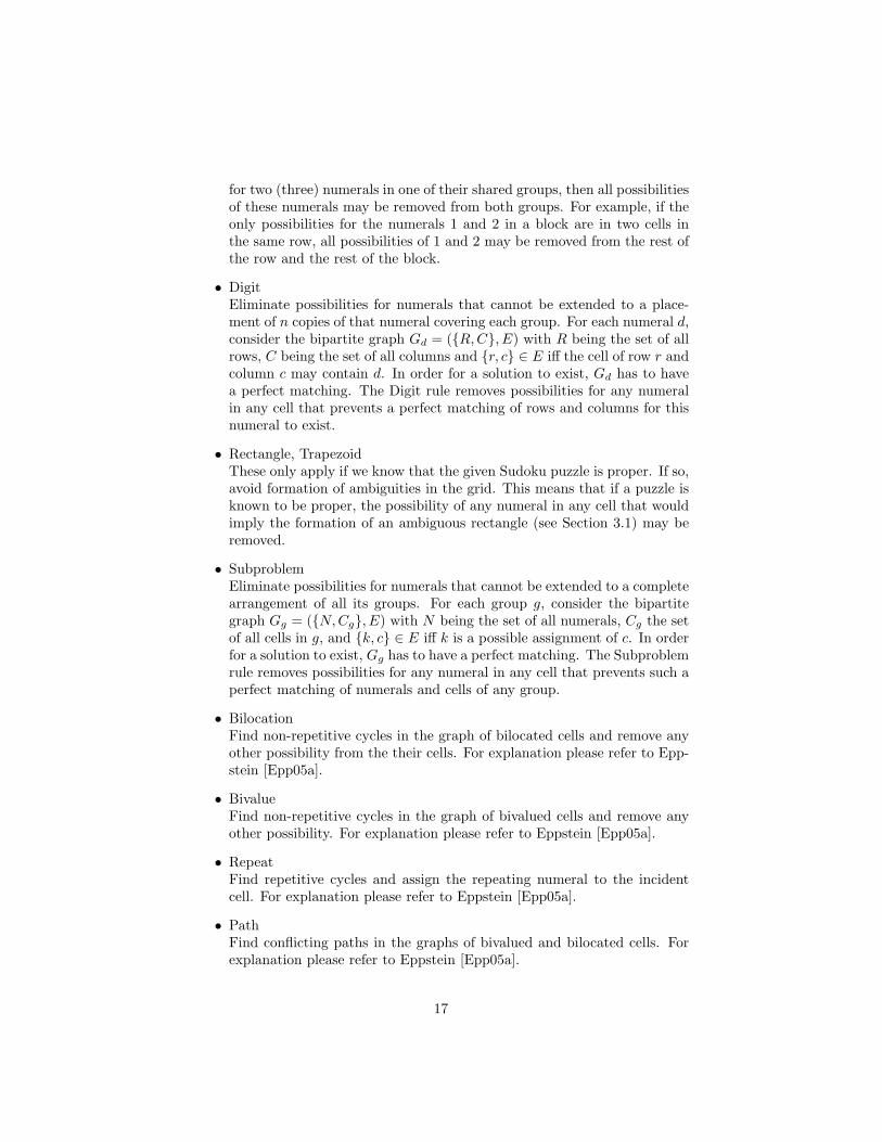
• DigitEliminate possibilities for numerals that cannot be extended to a place-ment of n copies of that numeral covering each group. For each numeral d,consider the bipartite graph Gd = (R,C, E) with R being the set of allrows, C being the set of all columns and r, c ∈ E iff the cell of row r andcolumn c may contain d. In order for a solution to exist, Gd has to havea perfect matching. The Digit rule removes possibilities for any numeralin any cell that prevents a perfect matching of rows and columns for thisnumeral to exist.

• Rectangle, TrapezoidThese only apply if we know that the given Sudoku puzzle is proper. If so,avoid formation of ambiguities in the grid. This means that if a puzzle isknown to be proper, the possibility of any numeral in any cell that wouldimply the formation of an ambiguous rectangle (see Section 3.1) may beremoved.

• SubproblemEliminate possibilities for numerals that cannot be extended to a completearrangement of all its groups. For each group g, consider the bipartitegraph Gg = (N, Cg, E) with N being the set of all numerals, Cg the setof all cells in g, and k, c ∈ E iff k is a possible assignment of c. In orderfor a solution to exist, Gg has to have a perfect matching. The Subproblemrule removes possibilities for any numeral in any cell that prevents such aperfect matching of numerals and cells of any group.

• BilocationFind non-repetitive cycles in the graph of bilocated cells and remove anyother possibility from the their cells. For explanation please refer to Epp-stein [Epp05a].

• BivalueFind non-repetitive cycles in the graph of bivalued cells and remove anyother possibility. For explanation please refer to Eppstein [Epp05a].

• RepeatFind repetitive cycles and assign the repeating numeral to the incidentcell. For explanation please refer to Eppstein [Epp05a].

• PathFind conflicting paths in the graphs of bivalued and bilocated cells. Forexplanation please refer to Eppstein [Epp05a].

17

With this ruleset, Eppstein managed to solve about 96% of the proper puzzlesgenerated by a puzzle generator that works as follows [Epp05b]:

1. generate a full Sudoku grid:

(a) choose a random cell

(b) assign a random, non-conflicting numeral

(c) propagate the changes by applying the most simple deduction rulesas often as possible

2. revert the changes step by step for as long as the puzzle stays proper(determined by a backtracking solver)

Solving by logic deduction is a suitable method to determine the difficulty of aSudoku puzzle, that is, how hard it is for a human solver to find a solution, forexample by applying a difficulty index to each deduction rule.

2.6 Graph Coloring

An n× n Sudoku grid may be interpreted as a graph in the following way: foreach cell there is a vertex of the graph. Each two vertices are connected iff theyshare a group. Each numeral is represented by a different color. A full Sudokugrid belongs to an n-coloring of this graph, so that no two adjacent verticeshave the same color. Solving a Sudoku puzzle is therefore equal to completing apartial coloring of the graph representing it. Note that this induces a reductionfrom Sudoku to Graph-n-Coloring: Given an n × n Sudoku puzzle, builda graph G with n2 vertices, one for each of the cells of the grid and connecttwo vertices iff they share at least one of their groups. The size of the graph ispolynomial in n and the partial coloring of G given by the hints in the Sudokupuzzle can be extended to an n-coloring of G iff the Sudoku puzzle has a solution.The number of ways to complete a partial coloring is a monic polynomial2 ofdegree at most n2 and due to the reduction, the same holds for the number ofdifferent solutions to a Sudoku puzzle [HM07]. Note that this is an exponentiallygrowing function in n.

3 Generalization and Contribution

In this chapter, the previously presented approaches will be extended and gener-alized. We will extend the term “essentially different” and consider the impactson the number of Sudoku grids. After presenting a different way to generateSudoku puzzles, we will introduce generalizations of parts of the set of deductionrules presented in Section 2.5.3 and a limited constraint propagation algorithmto solve Sudoku puzzles.

2A polynomial is called monic if all its coefficients are integer.

18

3.1 Counting Sudoku

In Section 2.1, the transformations leading to the term “essentially differentgrid” are mentioned. Recall also the difference between two Sudoku grids beingequal with respect to E′ and being equal with respect to E. Additionally to thefour transformations considered by E′, the ambiguous rectangle transformationmay be taken into account:

Definition An ambiguous rectangle is a formation of four cells that share ex-actly two different rows, columns, blocks, and numerals.

Flipping such a rectangle means to replace the content of each cell with thecontent of the cell it shares a block with.

Remark Figure 9 on page 10 shows an ambiguous rectangle (the gray cells formone) and its flipped variant. This is exactly the same as Eppstein [Epp05a] de-fined to test whether a Sudoku grid was ambiguous (a grid is ambiguous if itcontains an ambiguous rectangle). If a solution to a Sudoku puzzle containsan ambiguous rectangle that is not part of the puzzle, this solution cannotbe unique, because the ambiguous rectangle may be flipped to obtain a sec-ond solution to the puzzle. Flipping a flipped ambiguous rectangle reverts thetransformation, thus, flipping is its own inverse transformation. The equivalencerelation that takes the five transformations mentioned so far into account willbe referred to as E′′.

As shown in Figure 9 on page 10, the only two essentially different 4×4 Sudokugrids are in fact equal under flipping an ambiguous rectangle. Hence, withrespect to E′′ there is just one equivalence class of 4 × 4 Sudoku grids (thismeans, there are no essentially different grids of this type), which in turn meansthat all 4 × 4 Sudoku grids can be obtained from a single one by applying aseries of the stated transformations.

It is now of interest how many full 9 × 9 Sudoku grids exist that are es-sentially different with respect to E′′. Unfortunately, applying the ambiguousrectangle transformation to 9× 9 Sudoku grids is not trivial. Using Burnside’slemma like Jarvis and Russel [RJ06a] did to calculate N ′9×9 (see Lemma 2.4 onpage 10) is not applicable to the ambiguous rectangle transformation, becauseof its dependency on numerals, not just geometric shapes. Thus, there is at themoment no better way than to look at all N ′9×9 = 5, 472, 730, 538 equivalenceclasses and checking all pairs of classes for equality by brute force. However, forthe sheer size of these classes it is overwhelmingly costly to handle them. In thefollowing, we will estimate how many comparisons it would take to calculate thenumber of different Sudoku grids taking the ambiguous rectangle transforma-tion into account. If the average number of grids in an equivalence class withrespect to E′ is

k ≈ N9×9

N ′9×9

=6.6 · 1021

5.4 · 109≈ 1.2 · 1012

and a uniform distribution of grids in each class is assumed, the estimatednumber of comparisons is N9×9/2, which is approximately 3.3 · 1021. Hence

19

even if we compared a trillion Sudoku grids per second it would take 104 yearsto finish calculation. However it is still interesting how many 9 × 9 grids areessentially different with respect to E′′, because from a list of these grids, itwould be possible to generate every valid 9× 9 Sudoku grid, which is useful forgenerating Sudoku puzzles.

3.2 Generating Sudoku Puzzles

As we have already seen, Sudoku puzzle generators employ backtracking whenthe puzzle becomes invalid while adding or removing a numeral. To avoid this,we will try to retrace the actions a potential solver would take to solve a Sudokupuzzle and reverse them to reconstruct a puzzle from a given Sudoku grid. Ofcourse there are multiple puzzles for a single grid. The idea is to select anavailable trace that is closest to a desired difficulty level whenever there aremultiple choices. This eliminates the need for backtracking in the generationprocess. However, a full Sudoku grid has to be obtained first.

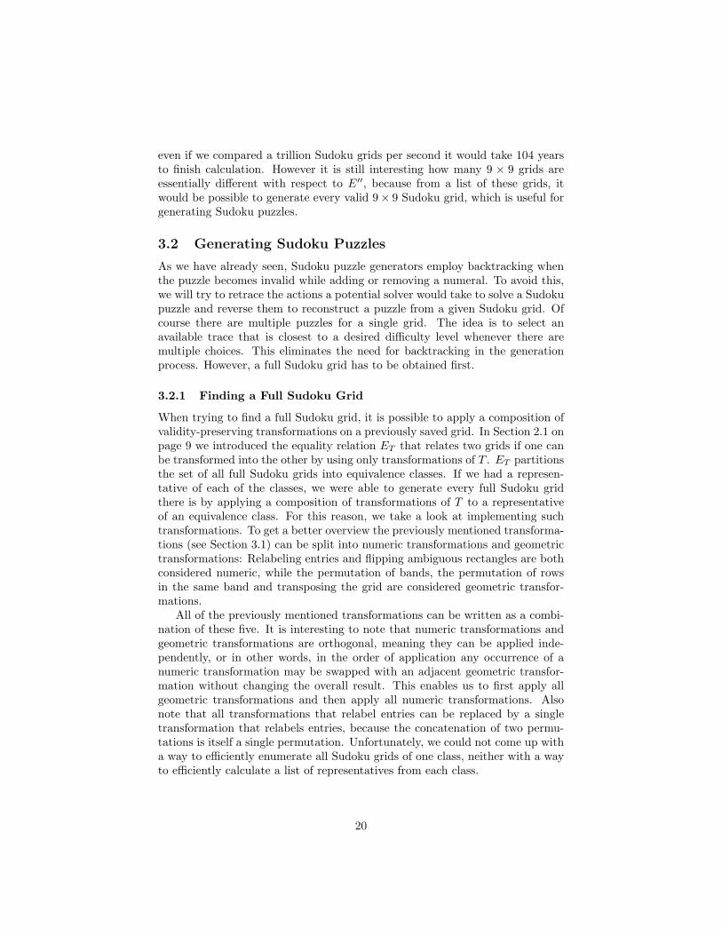
3.2.1 Finding a Full Sudoku Grid

When trying to find a full Sudoku grid, it is possible to apply a composition ofvalidity-preserving transformations on a previously saved grid. In Section 2.1 onpage 9 we introduced the equality relation ET that relates two grids if one canbe transformed into the other by using only transformations of T . ET partitionsthe set of all full Sudoku grids into equivalence classes. If we had a represen-tative of each of the classes, we were able to generate every full Sudoku gridthere is by applying a composition of transformations of T to a representativeof an equivalence class. For this reason, we take a look at implementing suchtransformations. To get a better overview the previously mentioned transforma-tions (see Section 3.1) can be split into numeric transformations and geometrictransformations: Relabeling entries and flipping ambiguous rectangles are bothconsidered numeric, while the permutation of bands, the permutation of rowsin the same band and transposing the grid are considered geometric transfor-mations.

All of the previously mentioned transformations can be written as a combi-nation of these five. It is interesting to note that numeric transformations andgeometric transformations are orthogonal, meaning they can be applied inde-pendently, or in other words, in the order of application any occurrence of anumeric transformation may be swapped with an adjacent geometric transfor-mation without changing the overall result. This enables us to first apply allgeometric transformations and then apply all numeric transformations. Alsonote that all transformations that relabel entries can be replaced by a singletransformation that relabels entries, because the concatenation of two permu-tations is itself a single permutation. Unfortunately, we could not come up witha way to efficiently enumerate all Sudoku grids of one class, neither with a wayto efficiently calculate a list of representatives from each class.

20

3.2.2 Deletion Witnesses

To decide whether the numeral in a certain cell may be removed it is of greatimportance whether it can be restored using the rules of a potential solver. Onepossibility would be to just try and remove that numeral. If the solver canderive it from the information left, it can be safely removed. However, thereis a better way than this trial and error technique. In the following, we willuse structures called deletion-witnesses (DW) to know in advance which rulesapplied on which cells would cause the numeral in a certain cell to be derived.

Definition A witness of a numeral k of a cell c is a pair (R,S) of a logic deduc-tion rule R and a set S of pairs of cells and numerals such that the collectivityof the pairs in S implies the assignment of k for the cell c by the rule R. Thenumeral k is then called witnessed by (R,S).

Remark Witnessed numerals may be removed in the generation process be-cause a solver can deduct them with the help of its witnesses.

This will enable us to remove only those numerals deductible by a given setof rules and thus effectively influencing the difficulty level of the puzzle. Thismethod still does not generally allow for choosing a difficulty level in advancebecause the rule that causes the deduction of the content of a selected cell is notnecessarily the easiest. Since the solver applies rules with a high difficulty ratingonly if the easier rules are exhausted, the puzzle may be easier than expected.However, a puzzle generated by this method will not be harder than expected.Also note that this method does not require backtracking.

3.3 Judging the Difficulty of Generated Sudoku Puzzles

When generating a Sudoku puzzle incrementally, the difficulty may be con-trolled by picking the numerals in such a way that deduction by rules with thedesired difficulty-level are possible. Whereas, when generating decrementally,the difficulty of the puzzle may be controlled by removing those numerals whoserecalculation has the desired difficulty.

3.4 Finding Solutions to Sudoku Puzzles

When looking at Eppstein’s Bilocation and Bivalue rules [Epp05a] a distinctfeeling that they are two occurrences of a common phenomenon arises. In ourwork, this phenomenon is called constraint propagation, meaning that changingthe grid in a certain way may affect other cells. However, not all possibleconstraint propagation mechanisms can be considered efficiently, hence we focuson four ways in which such propagation may occur:

1. Not assigning a numeral to a certain cell may force not assigning anothernumeral to another cell.

2. Not assigning a numeral to a certain cell may force assigning anothernumeral to another cell.

21

3. Assigning a numeral to a certain cell may force not assigning anothernumeral to another cell.

4. Assigning a numeral to a certain cell may force assigning another numeralto another cell.

In fact, Eppstein’s Bilocation and Bivalue rules [Epp05a] only cover points 2 (bythe Bilocation rule) and 4 (by the Bivalue rule). Additionally, the Bilocationand Bivalue rules are separated from one another, which further limits theirpotential. A cycle of Bivalued and Bilocated cells in a puzzle may exercisea constraint on other cells of the puzzle. This source of information is notexploited by applying Bivalue and Bilocation rules separately. Therefore thenext two sections will discuss a combination of these two. In Section 3.4.3,we will discuss a further step of generalization and the implementation of allmentioned rules.

3.4.1 Extension of Bilocation and Bivalue

Inspired by Eppstein’s cycle analysis approach [Epp05a] Bivalue and Bilocationrules were combined. This is possible since they are, as described above, con-straint propagating rules. The combination of the two rules can be condensedinto two rules for a human Sudoku solver. In the following, those are going tobe explained.

Definition If two cells c1,c2 in a group share a possible numeral x, these twocells are called grouped by x (written as c1 ∼g

x c2). If c1 ∼gx c2 and x cannot

be assigned to any other cell in the group, these two cells are called bilocated byx (written as c1 ∼l

x c2). If c1 ∼gx c2 and c1,c2 have only two possible numerals

each, the two cells are called bivalued by x (written as c1 ∼vx c2).

Remark Note that for two cells to be bivalued, the intersection of the sets oftheir respective possible numerals may contain both numerals, although this isnot required for the Bivalued property to apply. Also note that the grouped,bilocated, and bivalued relations are symmetric and intransitive.

Definition For an n× n Sudoku grid S, the graph G = (W, E) with

W = c | c is a cell in S

E = c, c′ | c, c′ ∈W ∧ ∃x(c ∼lx c′ ∨ c ∼v

x c′)

with the edge-labeling function

label : E → P(L, V × 1, . . . , n)

(L, x) ∈ label(c, c′)⇔ c ∼lx c′

(V, x) ∈ label(c, c′)⇔ c ∼vx c′

22

is called Force-Propagation-Graph or short FPG. Note that an edge may havemultiple labels. Let (x, y) be a label, then x = type((x, y)) is the type of thelabel and y = numeral((x, y)) is the numeral of the label. The function

d : (L, V × 1, . . . , n)2 → N

calculates the distances of two labels. It is much like the Hamming-Distance inthat it specifies how many parts of the labels differ.

d((p, q), (x, y)) =

0 , if p = x ∧ q = y

1 , if p = x⇔ q 6= y

2 , else.

A path in the FPG of length p + 2 is called alternating if for each edge ei in thepath, there is a label bi ∈ l(ei) such that

∀i ∈ 0, . . . , p : d(bi, bi+1) = 1.

That means that only one part of the label may differ from edge to edge. Analternating cycle is defined analogously.

The additional rules are defined as follows.

1. Alternating Cycle Rule (ACR)Suppose there is an alternating cycle in the FPG. Let ci be a cell of thecycle and ei and ei+1 its incident edges. If there are two numerals xand y with (L, x) ∈ label(ei) and (L, y) ∈ label(ei+1), remove all possiblenumerals except x and y from consideration for ci (see Figure 13).

2. Repetitive Cycle Rule (RCR)Suppose there is an alternating path of p+ 1 edges in the FPG that startsand ends at the same vertex (cell) but is not an alternating cycle - thismeans that the edges incident to the starting cell prevent the alternatingpath from being an alternating cycle. Let e0, ep denote these two edgesand b0, bp the labels of e0 and ep that were used to form the alternatingpath (note that d(b0, b1) = d(bp−1, bp) = 1, but d(b0, bp) 6= 1). Then, thestarting cell may not be assigned the numeral of the label whose type is Vif there are any, and must be assigned the numeral of the label whose typeis L if there are any. These two numerals cannot be the same because theequality would yield d(b0, bp) = 1 and thus the alternating path would aswell be an alternating cycle. Also, if both labels were of the same type,then for the same reason, their numerals would not differ.

While being an improvement to applying the Bilocation and Bivalue rules sepa-rately, the Alternating Cycle and Repetitive Cycle rules alone are not powerfulenough to provide a substantial gain of solving power, as shown in Section 4.Further generalization of the rules will be considered in the following sections.

23

7 5 8 4 6 98 4 6 5 1

3 7 2 8 5 45 6 3

5 2 13 9 65 8 4 61

5 1

Figure 13: An example for the application of the ACR. The grid on the rightshows the alternating cycle and the labels of its edges. Note the two markedcells in the top row. The left one may only contain 1 or 2, whereas the right onemay only contain 1 or 3. Because each of them may only contain two numeralsone of which is 1, the two cells are connected by an edge labeled “V1”, whichstands for “bivalued by 1”, with respect to the top row. That means that byassigning 1 to any of them, the other cell is forced not to contain 1 but theother possible numeral. Not being able to contain the 1 propagates by the edgelabeled “L1”. This label means that the two cells are bilocated by 1 with respectto their group, meaning that if 1 cannot be assigned to any of them, the othercell is forced to contain 1. The other edges are formed in the same manner.

24

3.4.2 Group-Modified Rules

The definition of the FPG can be extended to support propagation throughgrouping. That means that propagation may occur among cells that do nothave to be bivalued or bilocated, but just in the same group. Since there are alot of cells that are related by being in the same group, the extended FPG willbe much bigger (although still polynomial in n) than the FPG. The size maybe too much for a human solver to handle, which is why this was not includedinto the (previous) definition of FPG. However, for an automated solver, this isstill of interest, so we will define the extended FPG in the following:

Definition For an n× n Sudoku grid S, the graph G∗ = (W, E∗) with

W = c | c is a cell in S

E∗ = c, c′ | c, c′ ∈W ∧ ∃x(c ∼gx c′

with the edge-labeling function

label∗ : E∗ → P(L, V, G × 1, . . . , n)

(L, x) ∈ label∗(c, c′)⇔ c ∼lx c′

(V, x) ∈ label∗(c, c′)⇔ c ∼vx c′

(G, x) ∈ label∗(c, c′)⇔ c ∼gx c′

is called extended Force-Propagation-Graph or short EFPG. The function

d∗ : (L, V, G × 1, . . . , n)2 → N

calculates the distance of two labels.

d∗((p, q), (x, y)) =

∞ ,if p = x = G ∧ q 6= y

0 , if (p = L⇔ x = L) ∧ q = y

2 , if (p = L⇔ x 6= L) ∧ q 6= y

1 , otherwise.

Analogous to FPG, a path in the EFPG of length p + 2 is called alternating iffor each edge ei in the path, there is a label bi ∈ label(ei) such that

∀i ∈ 0, . . . , p : d∗(bi, bi+1) = 1.

Now, both additional rules stated in the previous section may also be used withd∗ instead of d:

1. Extended Alternating Cycle Rule (EACR)Suppose there is an alternating cycle in the FPG. Let ci be a cell of thecycle and ei and ei+1 its incident edges. If there are two numerals xand y with (L, x) ∈ label(ei) and (L, y) ∈ label(ei+1), remove all possiblenumerals except x and y from consideration for ci.

25

2. Extended Repetitive Cycle Rule (ERCR)Suppose there is an alternating path of p + 1 edges in the EFPG thatstarts and ends at the same vertex (cell) but is not an alternating cycle.Let e0, ep denote the two edges that are incident to the starting cell andb0, bp the labels of e0 and ep that were used to form the alternating path(note that d∗(b0, b1) = d∗(bp−1, bp) = 1 but ∞ 6= d∗(b0, bp) 6= 1). Thenthe starting cell may not be assigned the numeral of the label whose typeis V or G if there are any, and must be assigned the numeral of the labelwhose type is L if there are any.

With the Extended Alternating Cycle and Repetitive Cycle Rules we are closerto the goal of making use of the four limited constraint propagation mechanismsmentioned in Section 3.4. However, there is still a more abstract formulationthan these two rules, which for example takes into account multiple cells havinginfluence on the content of a single cell. In the following we will introduce thisformulation and explain our implementation of it.

3.4.3 Limited Constraint Propagation

After uniting Bilocation and Bivalue rules, there are still unconsidered con-straint propagation rules as mentioned in Section 3.4. To take them into ac-count a limited constraint propagation algorithm was implemented. The ideais to build a graph by analyzing the Sudoku grid with respect to the followinginterpretation of the fundamental rules of Sudoku:

• Each cell contains at least one numeral.This implies that, if there is only one numeral left for a cell, it has to beassigned to it (Eliminate).

• Each cell contains at most one numeral.This implies that, if a numeral has been assigned to a cell, no other numeralmay be assigned to it (Cell-Flood).

• Each group contains each numeral at least once.This implies that, if a numeral can only be assigned to one cell in a group,it has to be assigned to this exact cell (Locate).

• Each group contains each numeral at most once.This implies that, if a numeral has been assigned to a cell in a group, noother cell in this group may be assigned this numeral (Group-Flood).

In the following the algorithm and its implementation will be described. Thegeneral structure of a constraint-propagation-node, or fp node is shown in Fig-ure 14. The assignment of a numeral to a cell of a Sudoku grid is representedby an fp node containing this numeral. Not assigning a certain numeral to acell is represented by an fp node whose numeral is negative. An fp node can betriggered, meaning that it was determined to be true, for example, if a cell mustcontain the numeral k, the triggered-property of the fp node of k in this cell is

26

Figure 14: An fp node has an array of triggers and an array of impacts.

set to true. If a numeral k of a cell has been determined to cause a violation ofthe above rules, the node of −k of this cell is triggered. Every fp node has a listof triggers. A trigger of a node f is a list of fp nodes that collectively imply f ,meaning that f is a logic consequence of the totality of all nodes of the trigger.Triggers have a type that describes the nature of its implication. Types may beEliminate, Locate, Cell-Flood and Group-Flood:

• Eliminate:For all k ∈ 1, . . . , n and all cells c of the grid, the totality of all negativenodes of c except the node of −k trigger the node of k of this cell, seeFigure 16.

• Cell-Flood:For all k ∈ 1, . . . , n and all cells c of the grid, the node of k triggers allnegative nodes of c except −k, see Figure 16.

• Locate:For all k ∈ 1, . . . , n, all groups g and all cells c of g, the totality of allnodes with the numeral −k of all cells of g except c trigger the node withk of c, see Figure 17.

• Group-Flood:For all k ∈ 1, . . . , n, all groups g and all cells c of g, the node of ktriggers all nodes with −k of all cells of g except c, see Figure 17.

Likewise, every node has a list of impacts, which point to the triggers it partic-ipates in (those have to be considered when changing the “triggered” propertyof a node). With this data structure it is possible to represent most of theimplications that assigning or not assigning a certain numeral to a certain cellmay have. The graph structure in which these constraints are organized isbuilt by the following algorithm:

for all cells c in the grid beginfor all possibilities k of c begin

27

Figure 15: An fp node may be triggered by several other fp nodes and may itselfhave impact on multiple fp nodes.

28

Figure 16: Illustration of the Eliminate and Cell-Flood implementation.

Figure 17: Illustration of the Locate and Group-Flood implementation.

f = fp_node(c, k)s = new setfor all possible negative numerals -m begin

if m != k then add fp_node(c, -m) to smake s an impact of f by Cell-Floodmake f a trigger for s by Eliminate

t = new setfor all groups g that contain c begin

for all cells d of g beginif d != c then add fp_node(d, -k) to s

make s an impact of f by Group-Floodmake f a trigger of s by Locate

Lemma 3.1 The size of the graph structure is polynomial in the size of theSudoku grid.

Proof Let n be the number of different numerals in the grid. Note that thenumber of groups is 3 and does not depend on n. Hence, in each run of theouter loops, 4 triggers and 4 impacts will be added, each of size O(n). Theouter loops will run O(n2) · O(n) times since there are n2 cells in a grid andeach cell contains at most 2n possibilities (−n, . . . , n \ 0). In total, thegraph structure will be of size O(n4).

The following algorithm is an implementation of the Limited Constraint Prop-agation method to solve Sudoku puzzles:

build the graph structure Gaccount for the given hintsdo

for all cells c in the grid begin

29

for all possibilities k of c beginf = fp_node(c, k)f’ = fp_node(c, -k)if f’ is a consequence of f in G then trigger f’

while changes occurred

Remark Being a consequence of f in G is determined by a modified BFS3

algorithm that gathers all consequences of f in a set while traversing the graph.A node f∗ is considered a consequence of f if any trigger of f∗ consists exclu-sively of nodes that are either triggered, a consequence of f , or f itself. Thisway, the solver will only trigger nodes that are logical consequences of nodesthat are triggered already. Hence at any given time, all triggered nodes areconsequences of the hints given in the puzzle and therefore, if the solver finds afull Sudoku grid, it is indeed the solution to the puzzle. Note that if a puzzleis ambiguous, no solution will be found. Triggering f ′ causes all impacts of f ′

that do not contain any more untriggered nodes to be triggered as well, whichmay induce a chain-triggering of multiple nodes. The node f is then deletedsince f represents the impossibility of f ′.

Lemma 3.2 The solver runs in polynomial time.

Proof Obviously, the inner for-loops will be executed at most O(n3) times.The outer while-loop will run for as long as nodes are being triggered. Sinceonce a node is triggered, it will not become untriggered again, and the size ofthe data structure containing all nodes is polynomial in n, the outer while-loopwill run a number of times that is polynomial in n. Finding a path in a graphof polynomial size will also take polynomial time and so will triggering a node.All in all, the worst case running time stays polynomial in n.

With this technique, we now have a more powerful polynomial time solvingmechanism that allows for the implementation of the AC, RC, EAC and ERCrules by limiting the set of edges that are subject to the path algorithm used:The Graph-Accessibility algorithm that finds a path in the graph structurewas modified to only use edges that imply its incident vertices to be bilocated,bivalued or, in case of the extended rules, grouped in such a way as describedin the respective sections: All Cell-Flood triggers are allowed, Locate and Elim-inate triggers are allowed only if the trigger contains at most one untriggerednode. If a Group-Flood trigger is encountered, the AC and RC implementationmakes sure that the cells of both nodes have only two possible numerals andthus imply a Bivalue rule. The EAC and ERC implementation makes sure thatno two Group-Flood triggers that do not imply Bivaluation are consecutive.

To show how Alternating Cycles are being detected and exploited, supposethere is an Alternating Cycle. Let c be a cell in the cycle having more thantwo possible numerals. Let x, y and z be three of them with x and y beingpart of the labels of the two incident edges used to form the cycle. The path

3breadth-first search

30

Strategy Test Puzzles Test Puzzles Solved

ACR and RCR 5464 6 (0.11%)EACR and ERCR 5464 4261 (78%)Limited Constraint Propagation 5464 5464 (100%)

Table 2: Comparison of the three solving strategies presented in Section 3.4.

algorithm will find a path from the node (c, z) to the node (c,−z) along thecycle, thereby removing z from consideration for this cell as proposed by theAlternating Cycle rule. To show how Repetitive Cycles are being detected andexploited, suppose there is an alternating path that starts and ends in the samecell c. If (V, z) is a label of the first or last edge that is used to form this path,then the path algorithm will find a path from the node (c, z) to (c,−z) therebyremoving z from consideration for this cell. If (L, z′) is such a label, then thepath algorithm will find a path from the node (c,−z′) to (c, z′) thereby removing−z′ from consideration for c and hence triggering (c, z′) as described in the RCRdefinition. The same holds for the extended versions of the two rules.

When applying Limited Constraint Propagation, the difficulty of a puzzlecan be estimated by modifying the path algorithm to always take the mostsimple available path and analyzing the structure of it. Overall length, averagenumber of untriggered nodes of the triggers, types of used triggers are examplefeatures that may contribute to measuring the difficulty of a path. Having animplementation for all three methods, we are now prepared to carry out someexperiments.

4 Experimental Results

In this section, the results of our implementation of the deduction rules men-tioned in Section 3.4 will be presented. In order to test the AC, RC, EAC andERC rules (see Section 3.4.1 and Section 3.4.2) we modified our implementationof the Limited Constraint Propagation algorithm according to Section 3.4.3. Allthree variants were tested as follows: A list of Sudoku puzzles that could notbe solved by Eppstein’s solver [Epp05b] was generated. A puzzle from this listwill be referred to as test puzzle. For each test puzzle and each of the threesolvers, the solver and Eppstein’s solver were run in turns until the puzzle wassolved or no more numerals could be determined. Only traditional 9 × 9 Su-doku puzzles were considered. All in all, 143262 Sudoku puzzles were generated,5646 of which were test puzzles (3.94%). The results are presented briefly inTable 2. Although the combination of the two rules did prove to be helpful insolving Sudoku puzzles (Figure 18 shows a Sudoku puzzle that is not solvableby Eppstein’s solver [Epp05b], but does contain an alternating cycle that yieldsa solution to the puzzle) it was rare that the AC and RC rules were enoughto solve a test puzzle. Only six test puzzles (0.11% of all test puzzles) provedto be solvable by applying the AC and RC rules. The EAC and ERC rules

31

1 9 2 3 66 9 7 4 83 2 8 5 6 1 9 7 41 3 6

2 6 55 9 3 66 9 5 2 3

9 6 4 78 6 9 5

Figure 18: An example test puzzle that is solvable by applying the AlternatingCycle Rule. The cycle shown on the right implies the removal of the possibilityof the numeral 3 in the lower left marked cell. Hence, the 3 is to be assigned tothe cell directly below it.

proved to substantially increase solving power. 4261 test puzzles (78%) couldbe solved using the implementation described above. As expected, the furthestgeneralization, the implementation of the limited constraint propagation algo-rithm was superior to the simpler cycle rules. In the test, it was able to solveall 5464 test puzzles. This result encourages the idea that this algorithm maybe able to solve all proper Sudoku puzzles. Additionally, since it is easy tocombine the limited constraint propagation algorithm with a rating system, itmay be an excellent choice for an implementation of a Sudoku puzzle generatoras described in Section 3.2.

5 Outlook and Future Work

While writing this article, the following tasks arose but were not addressed here.They provide a topic for future research regarding Sudoku:

1. Compare generated puzzles with those of other generators (need somethingto measure quality, for example: number of filled cells).

2. Think about how to generate a full Sudoku grid (efficiently enumerateall?).

3. Find a suitable parameter and check whether Sudoku is FPT and deter-mine the problem kernel.

4. Calculate the number of different Sudoku grids under ambiguous rectangletransformation.

32

5. Consider Sudoku as convincing someone that a certain solution is indeedunique to a puzzle.

6. Research backtracking by Knuth’s dancing links.

7. Check hints of a incremental generator for superfluousness.

8. Try to prove that Limited Constraint Propagation can solve all properSudoku puzzles.

9. Implement a Sudoku generator based on deletion witnesses with regard tothe LCP-solver.

In the process of developing generalizations of previously researched topics, therewere dead ends and ideas that proved wrong. Attempts of extending the set oftransformations further than just adding the ambiguous rectangle failed: Inter-preting the n’th numeral in the m’th row as the row of the numeral n in thecolumn m failed because the resulting grid may have the same numeral twice ina block. However, this may work for Latin Squares. Secondly, switching rowswith blocks instead of switching rows and columns (as a transposition does),failed because each block intersects a row and a column with three numeralseach, if this block were to become a row, it would have to be intersected bytwo groups at 3 numerals each while there would have to be a cell shared by allthree groups, which is impossible if the overall geometry of the group was to bekept.

References

[Dud02] Henry Ernest Dudeney. The Canterbury Puzzles. Dover Publications,2002.

[Epp05a] David Eppstein. Nonrepetitive Paths and Cycles in Graphs with Ap-plication to Sudoku. ACM Computing Research Repository, July2005.

[Epp05b] David Eppstein. PADS library, July 2005. source code of sudoku.py,URL: http://www.ics.uci.edu/~eppstein/PADS/Sudoku.py.

[FJ06] Bertram Felgenhauer and Frazer Jarvis. Mathematics of Sudoku I.Mathematical Spectrum, 39, February 2006.

[HM07] Agnes M. Herzberg and Ram M. Murty. Sodoku Squares and Chro-matic Polynomials. Notices of the AMS, 54:708–717, June 2007.

[Mon05] Christopher Monckton. Sudoku X Book 1: The Only Puzzles Withthe X Factor. Justin, Charles & Co., Nov 2005.

[Pet06] Kjell Fredrik Pettersen. Sudoku Enumeration 2x5. URL: http://www.afjarvis.staff.shef.ac.uk/sudoku/sud25gp.html, 2006.

33

[PMH06] Caroline Higgins Peter M. Higgins. The Official Book of CircularSudoku: Book 1. Plume, July 2006.

[RJ06a] Ed Russel and Frazer Jarvis. Mathematics of Sudoku II. MathematicalSpectrum, 39, February 2006.

[RJ06b] Ed Russel and Frazer Jarvis. Sudoku Enumeration 2x3. URL: http://www.afjarvis.staff.shef.ac.uk/sudoku/sud23gp.html, 2006.

[Rus06] Ed Russel. Sudoku Enumeration 2x4. URL: http://www.afjarvis.staff.shef.ac.uk/sudoku/sud24gp.html, 2006.

[Sem05] Ivan Semeniuk. Addictive, seductive, sudoku. New Scientist, 2531,December 2005.

[Tel06] The Daily Telegraph. The ”Daily Telegraph” Samurai Sudoku. PanBooks, Oct 2006.

[YS03] Takayuki Yato and Takahiro Seta. Complexity and Completenessof Finding Another Solution and Its Application to Puzzles. IE-ICE transactions on fundamentals of electronics, communications andcomputer sciences, 86(5):1052–1060, 2003.

34