ORIGINAL ARTICLE

Coupling inter-patch movement models and landscape graphto assess functional connectivity

Benjamin Bergerot • Pierline Tournant • Jean-Pierre Moussus •

Virginie-M. Stevens • Romain Julliard • Michel Baguette •

Jean-Christophe Foltete

Received: 12 April 2012 / Accepted: 16 October 2012

� The Society of Population Ecology and Springer Japan 2012

Abstract Landscape connectivity is a key process for

the functioning and persistence of spatially-structured

populations in fragmented landscapes. Butterflies are

particularly sensitive to landscape change and are excel-

lent model organisms to study landscape connectivity.

Here, we infer functional connectivity from the assess-

ment of the selection of different landscape elements in a

highly fragmented landscape in the Ile-de-France region

(France). Firstly we measured the butterfly preferences of

the Large White butterfly (Pieris brassicae) in different

landscape elements using individual release experiments.

Secondly, we used an inter-patch movement model based

on butterfly choices to build the selection map of the

landscape elements to moving butterflies. From this map,

functional connectivity network of P. brassicae was

modelled using landscape graph-based approach. In our

study area, we identified nine components/groups of

connected habitat patches, eight of them located in

urbanized areas, whereas the last one covered the more

rural areas. Eventually, we provided elements to validate

the predictions of our model with independent experi-

ments of mass release-recapture of butterflies. Our study

shows (1) the efficiency of our inter-patch movement

model based on species preferences in predicting complex

ecological processes such as dispersal and (2) how inter-

patch movement model results coupled to landscape graph

can assess landscape functional connectivity at large

spatial scales.

Keywords Dispersal � Fragmented landscape �Inter-patch movement modelling � Lepidoptera �Pieris brassicae � Urbanization

Introduction

Habitat fragmentation is defined as the emergence of dis-

continuities in the habitat of a given species (Wilcove et al.

1986; Fahrig 2003; Haddad and Tewksbury 2005). From an

organism’s viewpoint, the fragmentation process creates a

patchwork of suitable habitats separated by a matrix of

landscape elements that are more or less hospitable

according to their resource availability or permeability to

movements. As habitat patches are often too small to

sustain viable populations, the persistence of many species

in fragmented landscapes relies on dispersal, i.e., the

movements of individuals which maintain gene flow

between local populations, rescue declining populations or

allow recolonizations after local extinction (Fahrig and

Merriam 1994; Haddad 1999; Hanski 1999).

B. Bergerot (&) � J.-P. Moussus � R. Julliard � M. Baguette

CNRS-MNHN-PARIS VI UMR 7204‘Conservation des

Especes, Restauration et Suivi des Populations’, CRBPO,

55 Rue Buffon, CP 51, 75005 Paris, France

e-mail: bergerot@mnhn.fr

B. Bergerot

Hepia, Centre de Lullier, University of Applied Sciences

Western Switzerland, Technology, Architecture and Landscape,

Route de Presinge 150, 1254 Jussy, Switzerland

P. Tournant � J.-C. Foltete

CNRS-UMR TheMA 6049, Universite de Franche-Comte,

32 rue Megevand, 25030 Besancon Cedex, France

V.-M. Stevens

F.R.S. FNRS, Unite de Biologie Du Comportement, Universite

de Liege, 22 quai Van Beneden, 4020 Liege, Belgium

V.-M. Stevens � M. Baguette

CNRS USR 2936 ‘Station d’ecologie experimentale du CNRS,

09200 Moulis, France

123

Popul Ecol

DOI 10.1007/s10144-012-0349-y

Landscape connectivity describes how elements making

up a given landscape will facilitate or impede the move-

ments of dispersing individuals (e.g., Taylor et al. 1993).

The mechanistic understanding of the dispersal process is

an essential prerequisite to the assessment of landscape

connectivity. Dispersal can be considered as a three-stage

process: (1) the decision of leaving a suitable habitat, (2)

the transience through more or less hospitable landscape

elements and (3) the settlement in an empty habitat or a

local population (Stevens et al. 2010). As various costs and

benefits are associated to each of these stages, they are

under uncoupled selection pressures (Baguette and Van

Dyck 2007; Clobert et al. 2009), which hinders wide

generalizations but rather makes functional landscape

connectivity population specific. Functional connectivity

ultimately results from habitat selection by dispersing

individuals (i.e., their choice at the border between land-

scape elements). Dispersal is itself controlled by the per-

meability of each landscape element (i.e., the relative costs

and benefits associated to their crossing; e.g., Stevens et al.

2006). Consequently, considering functional connectivity

requires dealing with individuals’ dispersal fluxes. If dis-

persal events are difficult to observe directly, dispersal

connectivity can be estimated using techniques such as

cost-distance modelling, individual based models or land-

scape genetics (Baguette and Van Dyck 2007; Spear et al.

2010; Storfer et al. 2010). Landscape graphs modelling

(applied from graph theory, Bunn et al. 2000, Urban and

Keitt 2001) has been proposed as an appealing addition to

these approaches and was used in many ecological studies

dealing with landscape connectivity for conservation pur-

poses (Saura and Pascual-Hortal 2007; Andersson and

Bodin 2009; Foltete et al. 2012). This method, based on the

metapopulation concept, allows modeling and measuring

the potential functional connectivity by taking into account

the whole network in a given landscape (Urban et al. 2009;

Galpern et al. 2011). The landscape is modelled as a graph

considering the optimal habitat patches for the focal spe-

cies as the nodes of the network and links between nodes

represent paths connecting habitat patches, based on eco-

logical assumptions about the movements of the species

within the landscape.

In this study, landscape graph modelling was associated

with an inter-patch movement model to assess the level

of functional connectivity between habitat patches (i.e.,

physical areas used by an organism or by a community of

different organisms, Morrison and Hall 2002) among

landscape elements (i.e., all other physical areas which

surround habitat patches) of an urbanized landscape around

Paris in the Ile-de-France region (France). More specifi-

cally, we intend to define and delineate graph components

(i.e., a group of connected nodes, isolated from other

components, also called a subgraph, Fall et al. 2007) within

this region for a study species, the Large White butterfly

(P. brassicae) and to test the relevance of these graph

components with empirical data from field study.

First, we experimentally assessed the landscape element

selection of individual butterflies. We released butterflies at

selected locations that offered choices between landscape

elements. Using the results of these experiments, we built a

transition matrix of the selections between landscape ele-

ments. Second, we used a graph-based approach to identify

graph components of highly connected habitat patches in

the region. Predictions were validated by using a mass

release experiment of marked individuals. We expected

that released individuals will move more often between

well connected habitat patches than between randomly

chosen landscape elements.

Materials and methods

Study species and rearing conditions

Pieris brassicae is a common and widespread species

across Europe (Bink 1992), which is present in the

urbanized region of Ile-de-France (Bergerot et al. 2010a).

We bred individuals in the lab by placing adults captured in

the region in an oviposition cage (80 9 80 9 80 cm) with

cabbage leaves (Brassica oleracea L.) under incandescent

light to maintain a 14L: 10D photoregime. A honey-water

solution (1:10 flower honey, 9: 10 water) in Eppendorf tube

was provided ad libitum as a source of carbohydrate, and

water was supplied through a soaked sponge. To produce

synchronized batches of young larvae, oviposition plants

were changed every 2 days. Eggs on plants were held in a

growth chamber at 23 �C and 50 % relative humidity until

larvae hatched and reached the adult stage. We then used

adult butterflies in the experiment.

Individual release procedure and habitat selection

Three release sites near Paris (France) were used to collect

individual data of habitat choice by butterflies in urbanized

landscapes (Fig. 1a). Each site was a 30 m diameter

roundabout covered with gravel without any tree (so

without any shaded area) or flowers (which could be

attractive for the butterflies). Each roundabout provided

access to different landscape elements with similar area,

hence offering the opportunity to select specific landscape

elements. As butterflies had to leave the roundabout, they

had to perform direct, oriented movements to enter a given

landscape element. Site 1 (IRS 1: 48�49037.6300N–

2�25050.5900E) offered escape through 6 landscape ele-

ments: lawn, shaded lawn (by trees), artificial area, shaded

artificial area (by trees), forest edge and wastelands

Popul Ecol

123

(Fig. 1b). Site 2 (IRS 2: 48�5005.1100N–2�26016.1800E)

offered escape through 4 different landscape elements:

lawn, shaded lawn, artificial area and shaded artificial area.

Finally, site 3 (IRS 3: 48�43048.0300N–2�31014.3200E)

offered 4 exits made of only two different landscape ele-

ments: lawn and shaded lawn.

We standardized the release procedure as much as pos-

sible. First, to insure comparable feeding status among

butterflies, butterflies were food-deprived during 12 h and

then fed them ad libitum with honey-water solution (1/10

honey, 9/10 water) during 2 h just before release. Butterflies

were placed in individual boxes at 5–6 �C for transportation

between the laboratory and the release sites (15–30 min

according to sites) to avoid stress and energy consumption.

All releases were performed under optimal weather condi-

tions to ensure butterfly flight activity: wind speed less than

10 km/h, air temperature C17 �C and 100 % sunshine. The

low wind speed prevented wind direction from interfering

with landscape element selection. For release, each butterfly

was individually placed on a take-off platform at the center

of the release point, with a random orientation relative to the

sun. Then, the butterfly was allowed to warm up for a few

minutes in the sun before it left the platform and escape the

roundabout. Only effective choice was considered i.e., when

the butterfly did not return to the roundabout within 10 s

after crossing its limit. We then recorded the first landscape

element in which it entered. The observers remained at a

distance C10 m from the butterfly to avoid interference with

the butterfly’s behavior.

We performed three release sessions in 2009 at each

site, at the end of May, mid-June and mid-July. In total, 48,

50 and 50 butterflies were released at sites 1, 2 and 3

respectively. Each session lasted 2 days in order to perform

the individual releases between 11.30 am and 14.30 pm in

specific weather conditions mentioned above. The order of

the sites was randomly chosen to avoid an hour effect.

Statistical analyses of butterfly preferences

To test if butterflies used some landscape elements more

than others, we compared the choices made at the three

sites (Table 1) using odd ratio comparisons. Odds ratio

comparisons describe the strength of the association of an

event (here the choice of a given landscape element)

a b

Fig. 1 Location of a the three individual release sites (IRS) and the two MRS used in the Ile-de-France region. b: IRS 1: roundabout with 6

landscape elements

Table 1 Butterfly leaving into each habitat (%) according to the

landscape elements present at each release site (N: number of indi-

viduals released in each site)

Site 1

(N = 48)

Site 2

(N = 50)

Site 3

(N = 50)

Lawn 20.83 26.00 32.00

Shaded lawn 4.17 56.00 68.00

Artificial area 2.08 4.00

Shaded artificial area 22.92 14.00

Wastelands 6.25

Forest edge 43.75

Popul Ecol

123

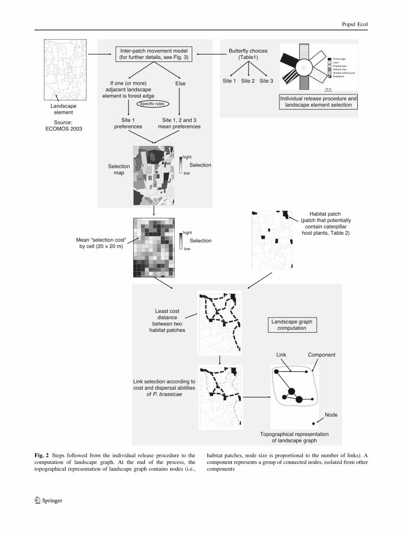
Fig. 2 Steps followed from the individual release procedure to the

computation of landscape graph. At the end of the process, the

topographical representation of landscape graph contains nodes (i.e.,

habitat patches, node size is proportional to the number of links). A

component represents a group of connected nodes, isolated from other

components

Popul Ecol

123

occurring in different groups (e.g., sites). To compare

butterfly preferences, we calculated the odds ratio and their

associated P values using median-unbiased estimation

(med-P).

Inter-patch movement model

The inter-patch movement model allowed the calculation

of ‘‘the number of individuals that come into a specific

landscape element’’ (i.e., selection of a landscape element

by P. brassicae) at the Ile-de-France scale to obtain a

‘‘selection map’’ (Fig. 2). More precisely, the model cal-

culated a percentage of individuals that come into a given

landscape element according to the nature of the landscape

element considered and the nature of the adjacent land-

scape elements (Fig. 3). Landscape elements data were

extracted from the land cover database (ECOMOS 2003,

Table 2). To compute the inter-patch model and so obtain

the selection map, we simulated the release of 200 but-

terflies in each landscape element and analyzed the pro-

pensity of butterflies to go in the adjacent elements (Fig. 3)

based on the butterfly preferences obtained from landscape

element selection results (i.e., individual release experi-

ments). In this model, the butterfly had two choices: ‘‘stay

in the landscape element’’ or ‘‘go in one of the adjacent

landscape elements’’. We thus obtained the percentage of

butterflies (out of 200 simulation releases per landscape

elements) which stay or leave the landscape element of

interest.

The inter-patch movement model follows specific rules

(Fig. 2). Firstly, some butterfly preferences could not be

tested in the individual release experiment (choice with

landscape elements classified as ‘‘Others’’ in Table 2, e.g.,

from/to inland waters). So in the inter-patch movement

model, we attributed the value 1 to butterfly selection

between landscape elements classified as ‘‘Others’’ and

available groups of landscape elements tested in individual

release experiment. By doing this, ‘‘Other’’ landscape

elements have no influence in the calculation of landscape

element selection.

Secondly, two specific rules (Fig. 2) were used to cal-

culate landscape element selection in the inter-patch

Fig. 3 Procedure of selection

(S) calculation for a landscape

element (Element) with 200

simulated releases in each

adjacent landscape element

Table 2 Number of landscape elements occurring in the study area following the ECOMOS 2003 classification and their cumulative area (ha)

Landscape element Description Number of elements

(%)

Cumulative area

(ha, %)

Artificial areas Tar roads, buildings, parking, houses, railway tracks 63306 (57.79 %) 79635.74 (30.90 %)

Shaded lawns Shaded lawnsa (public and private), cemeteriesa, campinga, orchardsa 24545 (22.40 %) 19765 (7.67 %)

Wastelands Shrubsa, industrial and urban wastelandsa, fallow landsa, construction

sites

8255 (7.53 %) 98031.97 (38.04 %)

Forest edges Forest edgesa, forest waysa 6225 (5.68 %) 45665.29 (17.72 %)

Lawns Lawnsa (in public and private areas), golf coursesa, racecoursesa, sport

facilitiesa4135 (3.77 %) 8343.43 (3.23 %)

Others Inland waters (rivers, ponds, lakes…) 2220 (2.02 %) 3131.99 (1.22 %)

Shaded artificial

areas

Shaded tar roads, shaded parking, artificial shaded canal banks 872 (0.81 %) 3148.25 (1.22 %)

a Landscape elements that potentially contain P. brassicae host plants and considered as habitat patch

Popul Ecol

123

movement model using results coming from the butterfly

preferences (i.e., individual release experiment). For one

specific landscape element, we used butterfly preferences

derived from butterfly choices at release site 1 (Table 1) if

an adjacent landscape element was forest edge, else we

used the mean butterfly preferences from all three sites.

Indeed, the individual release results showed that the

presence of forest edge in one adjacent landscape element

significantly modifies butterfly preferences and forest edge

was significantly more chosen. In other words, if the sur-

rounding landscape elements included forest edges, but-

terfly preferences considered in the inter-patch movement

model were derived from butterfly preferences at release

site 1, otherwise we used mean selections from all three

release sites (1, 2 and 3).

Thirdly, we weighted butterfly selection according to the

contact length between adjacent landscape elements. The

aim of this step was to take into account the contact length

between a specific landscape element and the adjacent

landscape elements in the calculation of butterfly selection

in the inter-patch movement model. For example, the

number of individuals that come in a specific landscape

element bordered at 80 % by shaded lawn and 20 % by

lawn would be different that the same landscape element

bordered at 20 % by shaded lawn and 80 % by lawn. We

thus assumed that the butterfly choice would increase with

the length of boundary between two adjacent landscape

elements.

Mass release-recapture protocol

To validate our model predictions, we performed two mass

releases of P. brassicae in 2009. Resightings of marked

butterflies were then mainly performed by volunteers made

aware of this experiment by wide media coverage (TV,

newspapers). Released butterflies were reared in the lab

under the same conditions as butterflies used in individual

release experiments. Adult butterflies were then placed in

transport cages (1.20 9 1.20 9 1.20 m) containing honey-

water solution and water 2 h before the release session

(travelling time was 20–35 min according to the location of

the release sites).

Two release sessions were performed, in two urban

parks: in park 1 in June 2009 and in park 2 in July 2009

under the same weather conditions as those selected for

individual releases Each mass release session began at

12.30 pm. Both parks were public urban parks (Fig. 1a).

Park 1 (MRS 1: 48�5108.3400N–2�1905.6800E) was 0.2 ha

and park 2 (MRS 2: 48�50038.6800N–2�21026.1500E) was

23.5 ha. 26 and 84 butterflies were released in MRS1 and

MRS2 respectively.

Each butterfly was marked on the ventral side of both

the left and the right hind-wings with fine, non-toxic,

permanent makers (Staedler Lumocolor 313, Staedler,

Nurnberg, Germany). Butterflies were marked with a

symbol associated with a specific colour for each mass

release site to increase the detection of reading errors. We

did not use individual marks to avoid identification mis-

takes as much as possible and because we wish to identify a

diffusion gradient in the matrix and not to get information

on individual trajectories.

Measuring landscape connectivity

In this study, we defined suitable habitat patches as landscape

elements that potentially contain caterpillar host plants

(Table 2). We used host plants and not nectar sources

because in urban landscapes, adult feeding resources do not

represent a main factor explaining butterflies distribution

patterns (Bergerot et al. 2010b). As P. brassicae females

mainly lay eggs on Brassica and Tropaeolum (Dennis and

Hardy 2007), we selected all landscape elements which

could contain these host plants in their herb layers in the

ECOMOS 2003 classification (Table 2).

Landscape connectivity network was investigated using

the landscape graph-based approach, considering the pre-

viously defined habitat patches as the node of the graph

(Fig. 2, Bunn et al. 2000; Urban and Keitt 2001). Among

the different types of existing graphs, we focused on the

minimum planar graph (O’Brien et al. 2006; Fall et al.

2007) for which all pairs of nearby nodes are connected by

a link based on least-cost distances. Various methods have

been proposed to model these inter-habitat patch links and

one of the most recurrent is based on least-cost distance

because of its greater ecological relevance than Euclidean

distance (O’Brien et al. 2006; Fall et al. 2007; Minor and

Lookingbill 2010). Based on the selection map obtained by

the inter-patch movement model (Fig. 2), we generated a

20 m resolution grid cell of our study area (Fig. 2) and

calculated the mean butterfly selection value of each cell.

These values were used to compute the edge-to-edge least

cost distance between all pairs of nearby nodes.

As in the studies of O’Brien et al. (2006) and Laita et al.

(2011) and in order to test how the landscape graph-based

model fits with the empirical data describing the dispersal

process, we drew several landscape graphs by successively

increasing the length of the least cost distance between

nodes (called the threshold distance). This length could

correspond to the maximum movement ability for the

considered species. Following this method, each landscape

graph newly computed contained a specific number of

components, i.e., a group of habitat patches potentially

interconnected by dispersal movements, functionally iso-

lated from any other group (Urban and Keitt 2001). The

threshold distance was initialized at 0, i.e., corresponding

to all the nodes remaining isolated, and was regularly

Popul Ecol

123

increased of 25 cost units until all the nodes were con-

nected into a single component. Between these two

extremes, the relevance of each graph was assessed by the

rate of intra-component resights, i.e., the proportion of

individuals visually recaptured in the same component

from where they were released (Fig. 4). Theoretically, we

assumed that the higher the proportion, the higher the

relevance of the graph. However, as the number of com-

ponents inherently decreases when the threshold distance

increases, we expect a monotonic increase in the proportion

of within-component recaptures with increasing threshold

distances. To distinguish an effect of landscape connec-

tivity from this artefact, we used a set of randomly gen-

erated resighting points to get a pattern purely attributable

to this artefact, and then compare observed patterns to this

null expectation. The spatial distribution (mean and stan-

dard deviation of Euclidean distances to mass release sites

(MRS) of those simulated points was the same as the real

resighting points. We simulated 100 resighting points for

each release site. Random resighting points were computed

based on the maximum number of days during which

butterflies were resighted for each release site and the mean

daily dispersal distance of P. brassicae (i.e., from 3 to 5

daily km randomly covered, Feltwell 1981). Then, we

compared recapture rates in the two series (real and sim-

ulated) using v2 tests according to increasing threshold

distances corresponding to decreasing number of compo-

nents. The most realistic landscape graph provides the

maximal difference between the rate of intra-component

resights resulting from the observed data and the random

sample. Indeed, at this threshold, the selected graph better

fitted the data than random simulations. Spatial and sta-

tistical analyses were performed with ESRI ArcGis 9.3�

and R2.7.0� respectively.

Results

Butterfly landscape element selection

Results showed no significant differences between butterfly

choices (Table 1) for lawns (same choices at sites 1, 2 and

3), artificial areas (sites 1 and 2) and shaded artificial areas

(sites 1 and 2). Only two significant differences occurred

between sites 1–2 and sites 1–3 (Table 1). Indeed, in sites 2

and 3, shaded lawns were significantly more chosen than in

site 1 (med-P \ 0.001). In site 1, forest edges were sig-

nificantly more chosen than other landscape elements

(v2 test, v2 = 36.5, df = 5, P \ 0.001). Thus, when forest

edges were available (site 1), butterflies preferentially

chose this landscape element, otherwise, when forest edges

were absent, they mainly chose shaded lawns (v2 test, site

2, v2 = 60.96, df = 3, P \ 0.001 and v2 test, site 3,

v2 = 6.48, df = 1, P = 0.011).

Landscape selection map

In the 20 9 20 meters grid obtained (Fig. 2), 64 % of the

landscape area were selected lower than 40 %. Only 21 %

a

b

Fig. 4 Rates of intra-component resights from real recapture points

(black line) and random recapture points (grey line) according to the

cost distance (meters) of landscape graphs (a). Difference between the

rates of intra-components resights from real recapture data and random

data according to the cost distance (meters) of landscape graphs (b)

Fig. 5 Frequency of the landscape elements selection (%) according

to their area (%) obtained by inter-patch movement modelling.

Although the category ‘0–10’ includes the value of zero, other

categories cover the range between the value above the lower limit

and the value at the higher limit

Popul Ecol

123

of landscape area had selection up to 50 % (Fig. 5). Based

on the ECOMOS classification of the putative presence of

host plants, 29 % of the landscape area were covered by

habitat patches (i.e., 34 % landscape elements among a

total of 109 558). The mean selection (%) of habitat pat-

ches was significantly higher (24.73 % ± 20.23) than

non habitat patches (9.59 % ± 9.52) (t test, t = 138,

P \ 0.001).

Mass-release-resighting experiment

and graph modelling

A total of 110 butterflies were released in two MRS (26 in

MRS 1 and 84 in MRS 2). 11 recapture events were

recorded (3 coming from MRS 1 and 8 coming from MRS

2, Fig. 6). Euclidean distances between release and

recapture sites varied from 120 m to 20.46 km and the

latest recapture was made 18 days after the release.

We calculated the unchanged component rates (i.e.,

number of butterflies seen in the same component) using

the 11 points where butterflies have been resighted and a

random sample of 100 points for each released site

(Fig. 4a).

The number of recaptures in the same graph components

was 5 individuals (45 %) for MRS 1 and MRS 2. For the

simulated data, the unchanged component rate was 14 %

(28 individuals). By comparing the unchanged component

rates made by graph components between real and simu-

lated data, we showed that resighted butterflies were

significantly more often found in the same component

than simulated individuals (v2 test, v2 = 5.62, df = 1,

P = 0.018).

The difference between these rates strongly varied

according to the butterfly selection: the curve of Fig. 4b

shows that the difference was positive until a cost distance

threshold of about 400, and then rapidly decreased to

become negative. According to this curve, we chose the

distance of 325 to compute the final landscape graph which

better represented the real P. brassicae habitat connectivity

network. By taking into account all the links having a least

cost distance between 300 and 325, the corresponding

value expressed in a metric unit was assessed to the aver-

age distance of 3.1 km. This graph identified 9 main

components in the landscape; the north of the region

(8 components) being much more fragmented than the

south (1 component) (Fig. 6a).

Discussion

Our results show that P. brassicae individuals mainly

chose forest edges and shaded lawns to leave their release

points, whereas open lawns were less frequently chosen.

The availability of nectar sources, roosting sites and gra-

dients of microclimatic conditions are key factors for the

selection of flyways by dispersing butterflies (e.g., Dennis

and Hardy 2007; Van Halder et al. 2008). In this study we

simulated individual inter-patch movements to obtain the

a b

Fig. 6 Map (a) of the 9 main

components (surrounded by

lines) and possible links (blacklines) between suitable habitats

(represented by circles with

various diameters according to

their areas). Resighting points of

released butterflies are related to

their release points (1 and 2 for

MRS 1 and MRS 2 respectively)

by black bold lines (For MRS 1,

two black bold lines are too

short to be seen). Urbanized

patches (in black) identified

(b) by the ECOMOS 2003

classification in the Ile-de-

France region (areas such as

rural patches and open urban

areas are represented in white)

Popul Ecol

123

selection value for each landscape element. Selection of

landscape elements varied widely in our urban region. This

result clearly shows that butterfly movements might be

hindered by hostile landscape elements in a densely

urbanized region such as Ile-de-France. Following Dennis

and Hardy (2007), two types of flights have been identified

for butterflies: ‘‘direct linear flight’’ regarded as dispersal

flight and ‘‘search flight’’ regarded as resource seeking

activity. Our inter-patch movement model was well suited

to model ‘‘direct linear flight’’ between landscape elements

because such displacements were shown to be widely used

by P. brassicae individuals in cities (Dennis and Hardy

2007).

In this study, landscape elements classified as ‘‘Others’’

have no influence in the calculation of landscape element

selection in the inter-patch movement model. Here, these

landscape elements represented only 1.22 % of the land-

scape elements considered and to our knowledge no other

studies revealed an impact of such landscape elements on

habitat selection in P. brassicae. Thus, we could easily

consider here that potential bias induced by such choice

was limited in our study. However, in other landscapes

where ‘‘Others’’ landscape elements could be more

numerous, care would need to be taken in the integration of

such parameters.

Compared to more classical work on dispersal (e.g.,

analysis of movement paths or random walk simulations,

Turchin 1998; Bowne and Bowers 2004), our method

provides new insights in the understanding of dispersal

behaviour by providing information how we can estimate

inter-patch movement of organisms in an environment and

also information on how we can estimate potential con-

nectivity between habitat patches. Indeed, if random walk

simulations within habitat patches provide a valuable tool

for modelling routine movements (Schtickzelle and Bagu-

ette 2003), for dispersal movements between landscape

elements at a larger scale, specific considerations are

required (i.e., butterfly landscape element selection). Thus,

as the contribution of routine movements to dispersal is

expected to decline with the degree of habitat fragmenta-

tion (Van Dyck and Baguette 2005), we then used inter-

patch movement modelling to landscape graph to predict

butterfly movements between habitat patches in our land-

scape. Methods based on such models are more appropriate

to coarser spatio-temporal scale methods than random walk

based methods (Turchin 1998) because both habitat patch

distribution and the nature of the matrix were taken into

account. It is particularly useful within the global change

context where attention is currently paid to urbanization

mediated landscape fragmentation (Stefanescu et al. 2004;

Ockinger et al. 2009). In such kind of landscapes, featuring

species’ most important dispersal ways (i.e., ecological

corridors, defined as spaces allowing species movements

between two hospitable patches, Clobert et al. 2001) will

favor the persistence of metapopulations by increasing

compensations of local extinction by immigration in dif-

ferent landscape elements (Hanski 1999). But, in urban

areas, factors such as strong boundary effect could limit

dispersal between habitat patches (Thomas 2000; Merckx

et al. 2003; Bergerot et al. 2012). In such a context, cou-

pling inter-patch movement models with landscape graphs

could be very useful to quantify boundary effects, to allow

the measurement of each landscape element contribution to

the overall connectivity (Urban and Keitt 2001; Saura and

Pascual-Hortal 2007) and to integrate individual behav-

iours into population models (Morzillo et al. 2011). Indeed,

the addition of parameters to our model could allow us to

answer demographic questions. For example, by adding

mortality and movement speed between landscape ele-

ments, we could generate specific predictions on how

spatio-temporal density of butterflies will change on a short

time scale.

By applying landscape graph to the study area, we

identified 9 graph components where habitat patches of

P. brassicae were well connected by permeable landscape

elements. Our comparison between the unchanged com-

ponent rates calculated from real and simulated resightings

showed that really resighted butterflies were significantly

more often found in the same component than simulated

individuals. If P. brassicae is considered as a really vagile

species (Bink 1992), the high number of graph components

in more urban areas (Fig. 6) shows that urbanization can

lead to the fragmentation of the landscape for this species.

The mean dispersal distance within a component averaged

to 3.1 ± 2.12 km. This distance was in accordance with

the dispersal distance of the species recorded in the liter-

ature (Feltwell 1981). So, in the Ile-de-France region, the

matrix was not so ‘‘inhospitable’’ for P. brassicae within a

component because our model (i.e., a combination between

dispersal abilities and nature of the landscape between

habitat patches) shows that the mean dispersal distance

within a component was approximately the mean daily

dispersal distance for this species. These results validate

the hypothesis previously made by Bergerot et al. 2010a

showing that dispersal abilities of P. brassicae allows the

persistence of this species in this region. We show that the

northern part of the study area, which is also the most

urbanized, is much more fragmented than its southern part

(Fig. 6a). The largest graph component identified in the

south could be explained by the nature of the landscape

elements. Indeed, urbanized areas are there mainly inter-

spersed with rural areas (Fig. 6b), which facilitate butterfly

movements.

Our aim was here to show how combining inter-patch

movement models and landscape graph-based approach

could provide an efficient tool to assess functional

Popul Ecol

123

connectivity in large areas by validating the results

obtained from this model with empirical data. According to

Urban et al. (2009) the validation of these models with

independent data is crucial. But in practice, several studies

using patch-based graph models suffer from a lack of

validation (Galpern et al. 2011). Providing this empirical

validation is not always feasible because of the difficulties

to obtain information about dispersal events in the field.

Combination of models such as inter-patch movement or

individual based models and landscape graphs is a useful

alternative to tackle this problem (Lookingbill et al. 2010;

Morzillo et al. 2011). Fortunately, the biological model

used in this study allows us to get field observation with

mass-release-resighting experiment. However, particular

attention has to be paid to our small number of resightings,

which forced us to combine the data from two different

sites. Indeed, statistical power to compare the rate of

recapture in the same component between recapture data

and simulated data is weak if we consider sites indepen-

dently. Only a global comparison is possible in our case

which limited our validation process. We are conscious of

the lack of real recapture events to fully validate our model.

However, even if 45 % of our real resights were made in

intra-components defined by our model (concerning only

11 individuals), a significant difference with the random

model was noticed. We could expect that the percentage of

intra-component resights would increase with the number

of individuals in the mass release experiment. If more

resightings had been available from more release sites, it

would have been possible to extend the conclusions of the

study by prioritizing their relative contributions to the

connectivity within their components.

This study reveals an appealing feature of the landscape

graph framework, i.e., the possibility of building maps of

functional connectivity and explore their structure with

small empirical data sets.

Acknowledgments We particularly thank volunteers for their

observation and participation to the study and Natureparif, Audrey

Coulon for the caterpillars rearing, Leyli Borner and all the Evoltrait

team based in Brunoy for their support and useful help in this study.

We especially thank the two anonymous reviewers whose comments

greatly improved this manuscript. MB’s contribution was funded by a

grant from the ANR (Agence Nationale de la Recherche, Open Call

DIAME 2008-2011 DIspersal And MEtapopulations). This project

was supported by the SCALE project. The graph analysis was con-

ducted in the framework of the Graphab project of the USR 3124

MSHE Ledoux, funded by the French Ministry of Ecology, Energy,

Sustainable Development and Sea.

References

Andersson E, Bodin O (2009) Practical tool for landscape planning?

An empirical investigation of network based models of habitat

fragmentation. Ecography 32:123–132

Baguette M, Van Dyck H (2007) Landscape connectivity and animal

behavior: functional grain as a key determinant for dispersal.

Landsc Ecol 22:1117–1129

Bergerot B, Julliard R, Baguette M (2010a) Metacommunity dynam-

ics: decline of functional relationship along a habitat fragmenta-

tion gradient. PLoS ONE 5(6):e11294. doi:10.1371/journal.pone.

0011294

Bergerot B, Fontaine B, Renard M, Cadi A, Julliard R (2010b)

Preferences for exotic flowers do not promote urban life in

butterflies. Landsc Urban Plan 96:98–107

Bergerot B, Merckx T, Van Dyck H, Baguette M (2012) Habitat

fragmentation impacts mobility in a common and widespread

woodland butterfly: do sexes respond differently? BMC Ecology

12(5). doi:10.1186/1472-6785-12-5

Bink BA (1992) Ecologische atlas van de Dagvlinders van Noord-

west-Europa (Ecological Atlas of the Butterflies of NW Europe).

Schuyt & Co, Haarlem

Bowne DR, Bowers MA (2004) Interpatch movements in spatially

structured populations: a literature review. Landsc Ecol 19:1–20

Bunn AG, Urban DL, Keitt TH (2000) Landscape connectivity: a

conservation application of graph theory. J Environ Manage

59:265–278

Clobert J, Danchin E, Dhont AA, Nichols JD (2001) Dispersal.

Oxford University Press, New York

Clobert J, Le Gaillard JF, Cote J, Meylan S, Massot M (2009)

Informed dispersal, heterogeneity in animal dispersal syndromes

and the dynamics of spatially structured populations. Ecol Lett

12:197–209

Dennis RLH, Hardy PB (2007) Support for mending the matrix:

resource seeking by butterflies in apparent non-resource zones.

J Insect Conserv 11:157–168

ECOMOS (2003) Ecological Soil Occupation Mode. See: http://www.

iau-idf.fr/lile-de-france/un-portrait-par-les-chiffres/occupation-du-

sol.html

Fahrig L (2003) Effects of habitat fragmentation on biodiversity.

Annu Rev Ecol Evol Syst 34:487–515

Fahrig L, Merriam G (1994) Conservation of fragmented populations.

Conserv Biol 8:50–59

Fall A, Fortin MJ, Manseau M, O’Brien D (2007) Spatial graphs:

principles and applications for habitat connectivity. Ecosystems

10:448–461

Feltwell J (1981) Large white butterfly: the biology, biochemistry,

and physiology of Pieris Brassicae. DRW junk publishers, The

Hague

Foltete J-C, Clauzel C, Vuidel G, Tournant P (2012) Integrating

graph-based connectivity metrics into species distribution mod-

els. Landsc Ecol 27:557–559

Galpern P, Manseau M, Fall A (2011) Patch-based graphs of

landscape connectivity: a guide to construction, analysis and

application for conservation. Biol Conserv 144:44–55

Haddad NN (1999) Corridor and distance effects on interpatch

movements: a landscape experiment with butterflies. Ecol Appl

9:612–622

Haddad NN, Tewksbury JJ (2005) Low-quality habitat corridors as

movement conduits for two butterfly species. Ecol Appl

15:250–257

Hanski I (1999) Metapopulation ecology. Oxford University Press,

New York

Laita A, KotiahoJ Monkkonen M (2011) Graph-theoretic connectivity

measures: what do they tell us about connectivity? Landsc Ecol

26:951–967

Lookingbill TR, Gardner RH, Ferrari JR, Keller CE (2010) Combin-

ing a dispersal model with network theory to assess habitat

connectivity. Ecol Appl 20:427–441

Merckx T, Van Dyck H, Karlsson B, Leimar O (2003) The evolution

of movements and behaviour at boundaries in different

Popul Ecol

123

landscapes: a common arena experiment with butterflies. Proc R

Soc B 270:1815–1821

Minor ES, Lookingbill TR (2010) A multiscale network analysis of

protected-area connectivity for mammals in the United States.

Conserv Biol 24:1549–1558

Morrison ML, Hall LS (2002) Standard terminology: toward a

common language to advance ecological understanding and

application. In: Scott JM, Heglund P, Morrisson ML, Raven PH

(eds) Predicting species occurrences. Issues of accuracy and

scale. Island Press, Washington, pp 43–52

Morzillo AT, Ferrari JR, Liu JG (2011) An integration of habitat

evaluation, individual based modeling, and graph theory for a

potential black bear population recovery in southeastern Texas,

USA. Landsc Ecol 26:69–81

O’Brien D, Manseau M, Fall A, Fortin MJ (2006) Testing the

importance of spatial configuration of winter habitat for wood-

land caribou: an application of graph theory. Biol Conserv

130:70–83

Ockinger E, Dannestam A, Smith HG (2009) The importance of

fragmentation and habitat quality of urban grasslands for

butterfly diversity. Landsc Urban Plan 93:31–37

Saura S, Pascual-Hortal L (2007) A new habitat availability index to

integrate connectivity in landscape conservation planning:

comparison with existing indices and application to a case

study. Landsc Urban Plan 83:91–103

Schtickzelle N, Baguette M (2003) Behavioural responses to habitat

patch boundaries restrict dispersal and generate emigration-patch

area relationships in fragmented landscapes. J Anim Ecol

72:533–545

Spear SF, Balkenhol N, Fortin MJ, McRae BH, Scribner K (2010)

Use of resistance surfaces for landscape genetic studies:

considerations for parameterization and analysis. Mol Ecol

19:3576–3591

Stefanescu C, Herrando S, Paramo F (2004) Butterfly species richness

in the north-west Mediterranean Basin: the role of natural and

human-induced factors. J Biogeogr 31:905–915

Stevens VM, Verkenne C, Vandewoestijne S, Wesselingh RA,

Baguette M (2006) Gene flow and functional connectivity in

the natterjack toad. Mol Ecol 15:2333–2344

Stevens VM, Turlure C, Baguette M (2010) A meta-analysis of

dispersal in butterflies. Biol Rev 85:625–642

Storfer A, Murphy MA, Spear SF, Holderegger R, Waits LP (2010)

Landscape genetics: where are we now? Mol Ecol 19:3496–3514

Taylor PD, Farhig L, Henein K, Merriam G (1993) Connectivity is a

vital element of landscape structure. Oikos 68:571–572

Thomas CD (2000) Dispersal and extinction in fragmented land-

scapes. Proc R Soc B 267:139–145

Turchin P (1998) Quantitative analysis of movement: measuring and

modeling population redistribution in animals and plants.

Sinauer Associates Inc, Sunderland

Urban D, Keitt T (2001) Landscape connectivity: a graph-theoretic

perspective. Ecology 82:1205–1218

Urban D, Minor ES, Treml EA, Schick RS (2009) Graph models of

habitat mosaics. Ecol Lett 12:260–273

Van Dyck H, Baguette M (2005) Dispersal behaviour in fragmented

landscapes: routine or special movements? Basic Appl Ecol

6:535–545

Van Halder I, Barbaro L, Corcket E, Jactel H (2008) Importance of

semi-natural habitats for the conservation of butterfly commu-

nities dominated by pine plantations. Biodivers Conserv

5:1149–1169

Wilcove DS, McLellan CH, Dobson AP (1986) Habitat fragmentation

in the temperate zone. In: Soule ME (ed) Conservation biology:

the science of scarcity and diversity. Sinauer Assoc, Sunderland,

pp 237–256

Popul Ecol

123