course 02402 introduction to statistics lecture 5
TRANSCRIPT

Course 02402 Introduction to Statistics
Lecture 5: Hypothesis testing
DTU ComputeTechnical University of Denmark2800 Lyngby – Denmark
Md Saifuddin Khalid (DTU Compute) Introduction to Statistics Spring 2021 1 / 37
Overview
1 Motivating example - sleep medicine
2 One-sample t-test and p-value
3 Critical value and relation to the confidence interval
4 Hypothesis tests in generalThe alternative hypothesisThe general methodErrors in hypothesis testing
5 Checking the normality assumptionThe normal q-q plotTransformation towards normality
Md Saifuddin Khalid (DTU Compute) Introduction to Statistics Spring 2021 2 / 37

Motivating example - sleep medicine
Overview
1 Motivating example - sleep medicine
2 One-sample t-test and p-value
3 Critical value and relation to the confidence interval
4 Hypothesis tests in generalThe alternative hypothesisThe general methodErrors in hypothesis testing
5 Checking the normality assumptionThe normal q-q plotTransformation towards normality
Md Saifuddin Khalid (DTU Compute) Introduction to Statistics Spring 2021 3 / 37
Motivating example - sleep medicine
Motivating example - sleep medicine
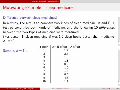
Difference between sleep medicines?
In a study, the aim is to compare two kinds of sleep medicine, A and B. 10test persons tried both kinds of medicine, and the following 10 differencesbetween the two types of medicine were measured:(For person 1, sleep medicine B was 1.2 sleep hours better than medicineA, etc.):
Sample, n = 10:person x = B effect - A effect
1 1.22 2.43 1.34 1.35 0.96 1.07 1.88 0.89 4.610 1.4
Md Saifuddin Khalid (DTU Compute) Introduction to Statistics Spring 2021 4 / 37
Motivating example - sleep medicine
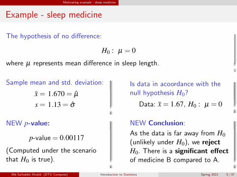
Example - sleep medicine
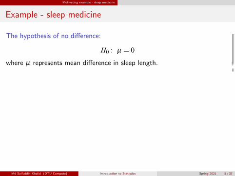
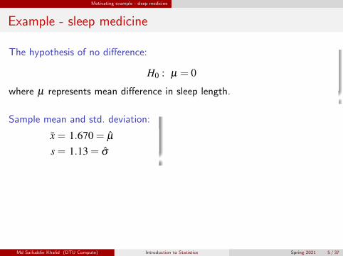
The hypothesis of no difference:
H0 : µ = 0
where µ represents mean difference in sleep length.
Sample mean and std. deviation:
x̄ = 1.670 = µ̂
s = 1.13 = σ̂
Is data in acoordance with thenull hypothesis H0?
Data: x̄ = 1.67, H0 : µ = 0
NEW p-value:
p-value= 0.00117
(Computed under the scenariothat H0 is true).
NEW Conclusion:
As the data is far away from H0(unlikely under H0), we rejectH0. There is a significant effectof medicine B compared to A.
Md Saifuddin Khalid (DTU Compute) Introduction to Statistics Spring 2021 5 / 37
Motivating example - sleep medicine
Example - sleep medicine
The hypothesis of no difference:
H0 : µ = 0
where µ represents mean difference in sleep length.
Sample mean and std. deviation:
x̄ = 1.670 = µ̂
s = 1.13 = σ̂
Is data in acoordance with thenull hypothesis H0?
Data: x̄ = 1.67, H0 : µ = 0
NEW p-value:
p-value= 0.00117
(Computed under the scenariothat H0 is true).
NEW Conclusion:
As the data is far away from H0(unlikely under H0), we rejectH0. There is a significant effectof medicine B compared to A.
Md Saifuddin Khalid (DTU Compute) Introduction to Statistics Spring 2021 5 / 37

One-sample t-test and p-value
Overview
1 Motivating example - sleep medicine
2 One-sample t-test and p-value
3 Critical value and relation to the confidence interval
4 Hypothesis tests in generalThe alternative hypothesisThe general methodErrors in hypothesis testing
5 Checking the normality assumptionThe normal q-q plotTransformation towards normality
Md Saifuddin Khalid (DTU Compute) Introduction to Statistics Spring 2021 6 / 37
One-sample t-test and p-value
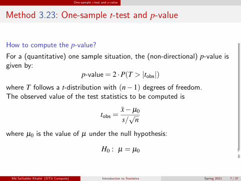
Method 3.23: One-sample t-test and p-value
How to compute the p-value?
For a (quantitative) one sample situation, the (non-directional) p-value isgiven by:
p-value= 2 ·P(T > |tobs|)where T follows a t-distribution with (n−1) degrees of freedom.The observed value of the test statistics to be computed is
tobs =x̄−µ0
s/√
n
where µ0 is the value of µ under the null hypothesis:
H0 : µ = µ0
Md Saifuddin Khalid (DTU Compute) Introduction to Statistics Spring 2021 7 / 37
One-sample t-test and p-value
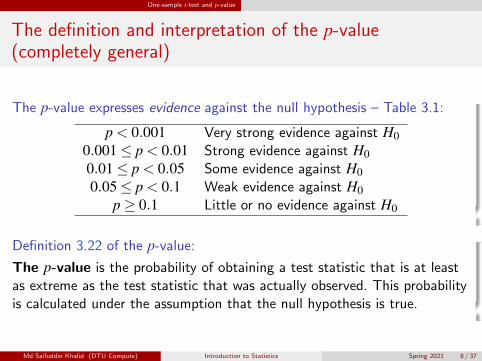
The definition and interpretation of the p-value(completely general)
The p-value expresses evidence against the null hypothesis – Table 3.1:
p < 0.001 Very strong evidence against H00.001≤ p < 0.01 Strong evidence against H00.01≤ p < 0.05 Some evidence against H00.05≤ p < 0.1 Weak evidence against H0
p≥ 0.1 Little or no evidence against H0
Definition 3.22 of the p-value:The p-value is the probability of obtaining a test statistic that is at leastas extreme as the test statistic that was actually observed. This probabilityis calculated under the assumption that the null hypothesis is true.
Md Saifuddin Khalid (DTU Compute) Introduction to Statistics Spring 2021 8 / 37
One-sample t-test and p-value
Example - sleep medicine
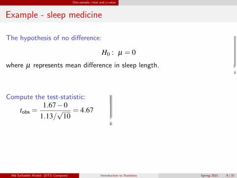
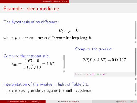
The hypothesis of no difference:
H0 : µ = 0
where µ represents mean difference in sleep length.
Compute the test-statistic:
tobs =1.67−0
1.13/√
10= 4.67
Compute the p-value:
2P(T > 4.67) = 0.00117
2 * (1 - pt(4.67, df = 9))
Interpretation of the p-value in light of Table 3.1:
There is strong evidence agains the null hypothesis.
Md Saifuddin Khalid (DTU Compute) Introduction to Statistics Spring 2021 9 / 37
One-sample t-test and p-value
Example - sleep medicine
The hypothesis of no difference:
H0 : µ = 0
where µ represents mean difference in sleep length.
Compute the test-statistic:
tobs =1.67−0
1.13/√
10= 4.67
Compute the p-value:
2P(T > 4.67) = 0.00117
2 * (1 - pt(4.67, df = 9))
Interpretation of the p-value in light of Table 3.1:
There is strong evidence agains the null hypothesis.
Md Saifuddin Khalid (DTU Compute) Introduction to Statistics Spring 2021 9 / 37

One-sample t-test and p-value
Example - sleep medicine - in R, manually
# Enter data
x <- c(1.2, 2.4, 1.3, 1.3, 0.9, 1.0, 1.8, 0.8, 4.6, 1.4)
n <- length(x) # sample size
# Compute 'tobs' - the observed test statistic
tobs <- (mean(x) - 0) / (sd(x) / sqrt(n))
# Compute the p-value as a tail-probability
# in the relevant t-distribution:
2 * (1 - pt(abs(tobs), df = n-1))
## [1] 0.001166
Md Saifuddin Khalid (DTU Compute) Introduction to Statistics Spring 2021 10 / 37

One-sample t-test and p-value
Example - sleeping medicine - in R, with built-in function
t.test(x)
##
## One Sample t-test
##
## data: x
## t = 4.7, df = 9, p-value = 0.001
## alternative hypothesis: true mean is not equal to 0
## 95 percent confidence interval:
## 0.8613 2.4787
## sample estimates:
## mean of x
## 1.67
Md Saifuddin Khalid (DTU Compute) Introduction to Statistics Spring 2021 11 / 37
One-sample t-test and p-value
Definition of a hypothesis test and significance (general)
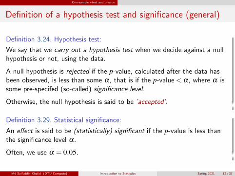
Definition 3.24. Hypothesis test:
We say that we carry out a hypothesis test when we decide against a nullhypothesis or not, using the data.
A null hypothesis is rejected if the p-value, calculated after the data hasbeen observed, is less than some α , that is if the p-value< α , where α issome pre-specifed (so-called) significance level.
Otherwise, the null hypothesis is said to be ’accepted’.
Definition 3.29. Statistical significance:
An effect is said to be (statistically) significant if the p-value is less thanthe significance level α .
Often, we use α = 0.05.
Md Saifuddin Khalid (DTU Compute) Introduction to Statistics Spring 2021 12 / 37
One-sample t-test and p-value
Example - sleep medicine
With α = 0.05:Since the p-value is less than α, we reject the nullhypothesis.
In conclusion:We have found a significant effect of medicine B whencompared to A (and B works better than A).
Md Saifuddin Khalid (DTU Compute) Introduction to Statistics Spring 2021 13 / 37

Critical value and relation to the confidence interval
Overview
1 Motivating example - sleep medicine
2 One-sample t-test and p-value
3 Critical value and relation to the confidence interval
4 Hypothesis tests in generalThe alternative hypothesisThe general methodErrors in hypothesis testing
5 Checking the normality assumptionThe normal q-q plotTransformation towards normality
Md Saifuddin Khalid (DTU Compute) Introduction to Statistics Spring 2021 14 / 37
Critical value and relation to the confidence interval
Critical value
Definition 3.31 - the critical values of the t-test:The (1−α)100% critical values for the (non-directional) one-sample t-testare the (α/2)100% and (1−α/2)100% quantiles of the t-distribution withn−1 degrees of freedom:
tα/2 and t1−α/2
Method 3.32: One-sample t-test by critical value:
A null hypothesis is rejected if the observed test-statistic is more extremethan the critical values:
If |tobs|> t1−α/2 then reject
otherwise accept.
Md Saifuddin Khalid (DTU Compute) Introduction to Statistics Spring 2021 15 / 37

Critical value and relation to the confidence interval
Critical value and hypothesis test
The acceptance region consists of the values of µ which are not too faraway from the sample mean - here on the standardized scale:
Acceptance
Rejection Rejection
t0.025 t0.9750Md Saifuddin Khalid (DTU Compute) Introduction to Statistics Spring 2021 16 / 37

Critical value and relation to the confidence interval
Critical value and hypothesis test
The acceptance region consists of the values of µ which are not too faraway from the sample mean - now on the original scale:
Acceptance
Rejection Rejection
x − t0.025s n x + t0.975s nxMd Saifuddin Khalid (DTU Compute) Introduction to Statistics Spring 2021 17 / 37
Critical value and relation to the confidence interval
Critical value, confidence interval and hypothesis test
Theorem 3.33: Critical value method = Confidence interval method
We consider a (1−α) ·100% confidence interval for µ :
x̄± t1−α/2 ·s√n
The confidence interval corresponds to the acceptance region for H0 whentesting the (non-directional) hypothesis
H0 : µ = µ0
(New) interpretation of the confidence interval:
The confidence interval covers those values of the parameter that webelieve in given the data.(Those values that we accept by the corresponding hypothesis test.)
Md Saifuddin Khalid (DTU Compute) Introduction to Statistics Spring 2021 18 / 37
Critical value and relation to the confidence interval
Proof:
Remark 3.34
A µ0 inside the confidence interval satisfies that
|x̄−µ0|< t1−α/2 ·s√n
which is equivalent to|x̄−µ0|
s√n
< t1−α/2
and again to|tobs|< t1−α/2
which then exactly states that µ0 is accepted, since the tobs is within thecritical values.
Md Saifuddin Khalid (DTU Compute) Introduction to Statistics Spring 2021 19 / 37
Hypothesis tests in general
Overview
1 Motivating example - sleep medicine
2 One-sample t-test and p-value
3 Critical value and relation to the confidence interval
4 Hypothesis tests in generalThe alternative hypothesisThe general methodErrors in hypothesis testing
5 Checking the normality assumptionThe normal q-q plotTransformation towards normality
Md Saifuddin Khalid (DTU Compute) Introduction to Statistics Spring 2021 20 / 37
Hypothesis tests in general The alternative hypothesis
The alternative hypothesis
So far - implied: (= non-directional)
The alternative to H0 : µ = µ0 is H1 : µ 6= µ0.
BUT there are other possible settings, e.g. one-sided (= directional), ”less”:
The alternative to H0 : µ = µ0 is H1 : µ < µ0.
We stick to the ”non-directional”in this course!
Md Saifuddin Khalid (DTU Compute) Introduction to Statistics Spring 2021 21 / 37

Hypothesis tests in general The general method
Steps of a hypothesis test - an overview
Generelly, a hypothesis test consists of the following steps:
1 Formulate the hypothesis and choose the level of significance α
(choose the ”risk-level”).
2 Calculate, using the data, the value of the test statistic.
3 Calculate the p-value using the test statistic and the relevantdistribution. Compare the p-value to the significance level α and makea conclusion.
OR:
Alternatively, make a conclusion based on the relevant critical value(s).
Md Saifuddin Khalid (DTU Compute) Introduction to Statistics Spring 2021 22 / 37
Hypothesis tests in general The general method
The one-sample t-test again
Method 3.36 The level α one-sample t-test:
1 Compute tobs as before.
2 Compute evidence against the null hypothesis H0 : µ = µ0 vs. thealternative hypothesis H1 : µ 6= µ0 by the
p–value= 2 ·P(T > |tobs|) ,
where the t-distribution with n−1 degrees of freedom is used.
3 If p-value< α , we reject H0. Otherwise, we accept H0.
OR:
The rejection/acceptance conclusion could alternatively, butequivalently, be made based on the critical value(s) ±t1−α/2:
If |tobs|> t1−α/2 we reject H0, otherwise we accept H0.
Md Saifuddin Khalid (DTU Compute) Introduction to Statistics Spring 2021 23 / 37
Hypothesis tests in general Errors in hypothesis testing
Errors in hypothesis testing
Two kind of errors can occur (but only one at a time!):
Type I: Rejection of H0 when H0 is true.Type II: Non-rejection (acceptance) of H0 when H1 is true.
The risks of the two types of errors are:
P(Type I error) = α
P(Type II error) = β
Md Saifuddin Khalid (DTU Compute) Introduction to Statistics Spring 2021 24 / 37
Hypothesis tests in general Errors in hypothesis testing
Court of law analogy
A man is standing in a court of law:
A man is standing in a court of law, accused of criminal activity.The null- and the alternative hypotheses are:
H0 : The man is not guilty.
H1 : The man is guilty.
Not being able to prove that the man is guilty is not the same as provingthat he is innocent.
Or, put differently:Accepting a null hypothesis is NOT a statistical proof of the nullhypothesis being true!
Md Saifuddin Khalid (DTU Compute) Introduction to Statistics Spring 2021 25 / 37
Hypothesis tests in general Errors in hypothesis testing
Errors in hypothesis testing
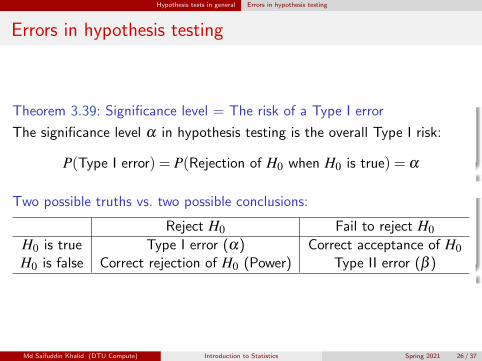
Theorem 3.39: Significance level = The risk of a Type I error
The significance level α in hypothesis testing is the overall Type I risk:
P(Type I error) = P(Rejection of H0 when H0 is true) = α
Two possible truths vs. two possible conclusions:
Reject H0 Fail to reject H0H0 is true Type I error (α) Correct acceptance of H0H0 is false Correct rejection of H0 (Power) Type II error (β )
Md Saifuddin Khalid (DTU Compute) Introduction to Statistics Spring 2021 26 / 37
Hypothesis tests in general Errors in hypothesis testing
Errors in hypothesis testing
Theorem 3.39: Significance level = The risk of a Type I error
The significance level α in hypothesis testing is the overall Type I risk:
P(Type I error) = P(Rejection of H0 when H0 is true) = α
Two possible truths vs. two possible conclusions:
Reject H0 Fail to reject H0H0 is true Type I error (α) Correct acceptance of H0H0 is false Correct rejection of H0 (Power) Type II error (β )
Md Saifuddin Khalid (DTU Compute) Introduction to Statistics Spring 2021 26 / 37

Checking the normality assumption
Overview
1 Motivating example - sleep medicine
2 One-sample t-test and p-value
3 Critical value and relation to the confidence interval
4 Hypothesis tests in generalThe alternative hypothesisThe general methodErrors in hypothesis testing
5 Checking the normality assumptionThe normal q-q plotTransformation towards normality
Md Saifuddin Khalid (DTU Compute) Introduction to Statistics Spring 2021 27 / 37

Checking the normality assumption The normal q-q plot
Example - student heights
# Student heights datax <- c(168, 161, 167, 179, 184, 166, 198, 187, 191, 179)
# Density histogram of student height data together with normal pdfhist(x, xlab = "Height", main = "", freq = FALSE)lines(seq(160, 200, 1), dnorm(seq(160, 200, 1), mean(x), sd(x)))
Height
Den
sity
160 170 180 190 200
0.00
0.01
0.02
0.03
0.04
Md Saifuddin Khalid (DTU Compute) Introduction to Statistics Spring 2021 28 / 37

Checking the normality assumption The normal q-q plot
Example - 100 observations from a normal distribution
# Density histogram of simulated data from normal distribution# (n = 100) together with normal pdfxr <- rnorm(100, mean(x), sd(x))hist(xr, xlab = "Height", main = "", freq = FALSE, ylim = c(0, 0.032))lines(seq(130, 230, 1), dnorm(seq(130, 230, 1), mean(x), sd(x)))
Height
Den
sity
140 150 160 170 180 190 200 210
0.00
00.
010
0.02
00.
030
Md Saifuddin Khalid (DTU Compute) Introduction to Statistics Spring 2021 29 / 37

Checking the normality assumption The normal q-q plot
Example - student heights - ecdf
# Empirical cdf for student height data together
# with normal cdf
plot(ecdf(x), verticals = TRUE)
xp <- seq(0.9*min(x), 1.1*max(x), length.out = 100)
lines(xp, pnorm(xp, mean(x), sd(x)))
160 170 180 190 200
0.0
0.2
0.4
0.6
0.8
1.0
ecdf(x)
x
Fn(
x)
Md Saifuddin Khalid (DTU Compute) Introduction to Statistics Spring 2021 30 / 37

Checking the normality assumption The normal q-q plot
Example - 100 observations from a normal distribution -ecdf
# Empirical cdf of simulated data from normal distribution
# (n = 100) together with normal cdf
xr <- rnorm(100, mean(x), sd(x))
plot(ecdf(xr), verticals = TRUE)
xp <- seq(0.9*min(xr), 1.1*max(xr), length.out = 100)
lines(xp, pnorm(xp, mean(xr), sd(xr)))
140 160 180 200
0.0
0.2
0.4
0.6
0.8
1.0
ecdf(xr)
x
Fn(
x)
Md Saifuddin Khalid (DTU Compute) Introduction to Statistics Spring 2021 31 / 37
Checking the normality assumption The normal q-q plot
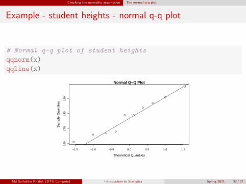
Example - student heights - normal q-q plot
# Normal q-q plot of student heights
qqnorm(x)
qqline(x)
−1.5 −1.0 −0.5 0.0 0.5 1.0 1.5
160
170
180
190
Normal Q−Q Plot
Theoretical Quantiles
Sam
ple
Qua
ntile
s
Md Saifuddin Khalid (DTU Compute) Introduction to Statistics Spring 2021 32 / 37

Checking the normality assumption The normal q-q plot
Normal q-q plot
Method 3.42- The formal definition
The ordered observations x(1), . . . ,x(n) are plotted versus a set of expectednormal quantiles zp1 , . . . ,zpn . Different definitions of p1, . . . ,pn exist:
In R, when n > 10:
pi =i−0.5
n, i = 1, . . . ,n
In R, when n≤ 10:
pi =i−3/8n+1/4
, i = 1, . . . ,n
Md Saifuddin Khalid (DTU Compute) Introduction to Statistics Spring 2021 33 / 37
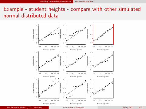
Checking the normality assumption The normal q-q plot
Example - student heights - compare with other simulatednormal distributed data
●
●
●
● ● ●
●
●
●
●
−1.5 −0.5 0.5 1.0 1.5
−2
−1
01
2
Theoretical Quantiles
Sam
ple
Qua
ntile
s
●●
●
●●
●
●
●
●
●
−1.5 −0.5 0.5 1.0 1.5
−2
−1
01
2
Theoretical Quantiles
Sam
ple
Qua
ntile
s
●
●
●
●
●
●
●
●
●
●
−1.5 −0.5 0.5 1.0 1.5
−2
−1
01
2
Theoretical Quantiles
Sam
ple
Qua
ntile
s
●
●
●
●
●
●●
●
●
●
−1.5 −0.5 0.5 1.0 1.5
−2
−1
01
2
Theoretical Quantiles
Sam
ple
Qua
ntile
s
●●
●
●
●
● ●
●
●
●
−1.5 −0.5 0.5 1.0 1.5
−2
−1
01
2
Theoretical Quantiles
Sam
ple
Qua
ntile
s●
●
●●
●
●
●
●
●
●
−1.5 −0.5 0.5 1.0 1.5
−2
−1
01
2
Theoretical Quantiles
Sam
ple
Qua
ntile
s
●
●
●
●
●
●
●●
●
●
−1.5 −0.5 0.5 1.0 1.5
−2
−1
01
2
Theoretical Quantiles
Sam
ple
Qua
ntile
s
●
●●
●●●
●
●
●
●
−1.5 −0.5 0.5 1.0 1.5
−2
−1
01
2
Theoretical Quantiles
Sam
ple
Qua
ntile
s
●
●
●
●
●
●
●
●
●●
−1.5 −0.5 0.5 1.0 1.5
−2
−1
01
2
Theoretical Quantiles
Sam
ple
Qua
ntile
s
Md Saifuddin Khalid (DTU Compute) Introduction to Statistics Spring 2021 34 / 37

Checking the normality assumption Transformation towards normality
Example - Radon data
## Reading in the data
radon <- c(2.4, 4.2, 1.8, 2.5, 5.4, 2.2, 4.0, 1.1, 1.5, 5.4, 6.3,
1.9, 1.7, 1.1, 6.6, 3.1, 2.3, 1.4, 2.9, 2.9)
## Histogram and q-q plot of data
par(mfrow = c(1,2))
hist(radon)
qqnorm(radon)
qqline(radon)
Histogram of radon
radon
Fre
quen
cy
1 2 3 4 5 6 7
01
23
45
67
−2 −1 0 1 2
12
34
56
Normal Q−Q Plot
Theoretical Quantiles
Sam
ple
Qua
ntile
s
Md Saifuddin Khalid (DTU Compute) Introduction to Statistics Spring 2021 35 / 37
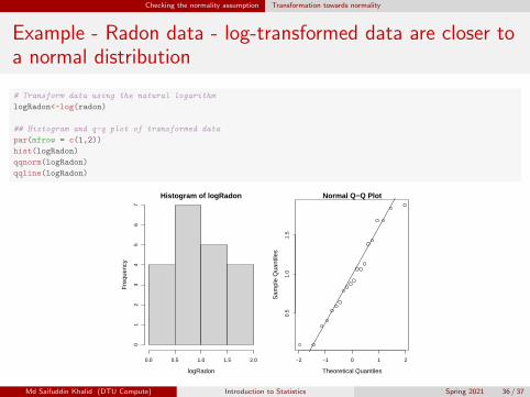
Checking the normality assumption Transformation towards normality
Example - Radon data - log-transformed data are closer toa normal distribution
# Transform data using the natural logarithm
logRadon<-log(radon)
## Histogram and q-q plot of transformed data
par(mfrow = c(1,2))
hist(logRadon)
qqnorm(logRadon)
qqline(logRadon)
Histogram of logRadon
logRadon
Fre
quen
cy
0.0 0.5 1.0 1.5 2.0
01
23
45
67
−2 −1 0 1 2
0.5
1.0
1.5
Normal Q−Q Plot
Theoretical Quantiles
Sam
ple
Qua
ntile
s
Md Saifuddin Khalid (DTU Compute) Introduction to Statistics Spring 2021 36 / 37
Checking the normality assumption Transformation towards normality
Agenda
1 Motivating example - sleep medicine
2 One-sample t-test and p-value
3 Critical value and relation to the confidence interval
4 Hypothesis tests in generalThe alternative hypothesisThe general methodErrors in hypothesis testing
5 Checking the normality assumptionThe normal q-q plotTransformation towards normality
Md Saifuddin Khalid (DTU Compute) Introduction to Statistics Spring 2021 37 / 37