course code: bfn728 course title: quantitative techniques ... · this course, bfn 728: quantitative...

NATIONAL OPEN UNIVERSITY OF NIGERIA

FACULTY OF MANAGEMENT SCIENCES

COURSE CODE: BFN728

COURSE TITLE: QUANTITATIVE TECHNIQUES FOR FINANCIAL

DECISIONS

Course Writers: Dr. Abdullahi S. Araga and Faith E. Onyebuenyi

Department of Financial Studies Faculty of Management Sciences

Course Editor: PROF.VINCENT EZEABASILIM

Department of banking and Finance

Anambra State University, Uli.

Programme Coordinator DR. OKOH JOHNSON IFEANYI

Department of Financial Studies

Faculty of Management Sciences

Head of Department Dr. Ofe. Inua

Department of Financial Studies

Faculty of Management Sciences

CONTENTS PAGE

Introduction ……………………………………………………… 1 Course Aims……………………………………………………….. 1

Course Objectives…………………………………………….…… 1 Course Materials…………………………………………….…….. 2

Study Units…………………….…………………………..…..…… 2 Assignments ……………………………………………………….... 3

Tutor-Marked Assignment…………………………....................... 3

Final Examination and Grading……………………….…………... 3

Summary ……………………………………………………………… 3

Introduction

This course, BFN 728: Quantitative Techniques for Financial Decisions is a two

credit unit compulsory course for students studying PGD banking and Finance and

other related programmes in the faculty of Management Sciences.

The course has been conveniently arranged for you in eighteen distinct but related

units of study activities. In this course guide, you will find out what you need to

know about the aims and objectives of the course, components of the course

material, arrangement of the study units, assignments, and examinations.

The Course Aim The course is aimed at acquainting you with what quantitative techniques are all about

and letting you understand the practical applications of quantitative techniques in

business and economic decision making. To ensure that this aim is achieved, some

important background information will be provided and discussed, including:

definition of quantitative techniques

uses of quantitative techniques

tools and applications of quantitative techniques

the correlation theory

forecasting and time-series analysis

index numbers

inventory control

decision analysis

network planning and analysis

arithmetic and geometric progression

interest rate and depreciation

present value and investment appraisals

The Course Objectives

At the end of the course you should be able to:

1. appreciate the uses and importance of quantitative methods in decision making;

2. formulate and solve decision problems in quantitative terms;

3. discuss business forecasts based on past data;

4. compute real monetary values for investment projects;

5. explain profitable inventory decisions; 6. plan network activities for productive business operations

Course Material The course material package is composed of:

The Course Guide

The Study Units

Self-Assessment Exercises

Tutor-Marked Assignments

References/Further Readings

The Study Units

The study units are as listed below:

Module 1

Unit 1 Uses, Importance, and Tools of Quantitative Techniques in Decision Making

Unit 2 Mathematical Tools I: Equation and Inequalities

Unit 3 Mathematical Tools I: Simultaneous Equations, Linear Functions, and Linear

Inequalities

Unit 4 Mathematical Tools II: Introduction to Matrix Algebra

Unit 5 Mathematical Tools III: Applied Differential Calculus

Module 2

Unit 1 Statistical Tool I: Measures of Averages

Unit 2 Statistical Tools II: Measures of Variability or Dispersion

Unit 3 Statistical Tools III: Sets and Set Operations

Unit 4 Statistical Tools IV: Probability Theory and Applications

Unit 5 Correlation Theory

Module 3

Unit 1 Forecasting and Time-Series Analysis

Unit 2 Index Numbers

Unit 3 Inventory Control

Unit 4 Decision Analysis

Unit 5 Network Planning and Analysis

Module 4

Unit 1 Arithmetic and Geometric Progression

Unit 2 Interest Rate and Depreciation

Unit 3 Present Values and Investment Analysis

Unit 4 Nature of Statistics

Unit 5 Sampling Techniques

Assignments Each unit of the course has a self assessment exercise. You will be expected to attempt

them as this will enable you understand the content of the unit.

Tutor-Marked Assignment The Tutor-Marked Assignments at the end of each unit are designed to test your

understanding and application of the concepts learned. It is important that these

assignments are submitted to your facilitators for assessments. They make up 30

percent of the total score for the course.

Final Examination and Grading

At the end of the course, you will be expected to participate in the final examinations

as scheduled. The final examination constitutes 70 percent of the total score for the

course.

Summary This course, BFN 728: Quantitative Techniques for Financial Decisions is ideal for

today’s computerised business environment. It will enable you apply quantitative

techniques in such business functions as planning, controlling, forecasting, and

evaluation. Having successfully completed the course, you will be equipped with the

latest global knowledge on business decisions. Enjoy the course.

.

Assignments

Each unit of the course has a self assessment exercise. You will be

expected to attempt them as this will enable you understand the content of

the unit.

Tutor-Marked Assignment

The Tutor-Marked Assignments at the end of each unit are designed to

test your understanding and application of the concepts learned. It is

important that these assignments are submitted to your facilitators for

assessments. They make up 30 percent of the total score for the course.

Final Examination and Grading

At the end of the course, you will be expected to participate in the final

examinations as scheduled. The final examination constitutes 70 percent

of the total score for the course.

Summary

This course, BFN 728: Quantitative Techniques for Financial Decisions is

ideal for today’s computerised business environment. It will enable you

apply quantitative techniques in such business functions as planning,

controlling, forecasting, and evaluation. Having successfully completed

the course, you will be equipped with the latest global knowledge on

business decisions. Enjoy the course.

MAIN COURSE

Course Code

Course Title

BFN 728

Quantitative Techniques for Financial Decisions

CONTENTS PAGE

Module 1…………………………………………………………. 1

Unit 1 Uses, Importance, and Tools of Quantitative

Techniques in Decision Making…………………….. 1

Unit 2 Mathematical Tools I: Equation and Inequalities…… 6

Unit 3 Mathematical Tools I: Simultaneous Equations,

Linear Functions and Linear Inequalities…………… 15

Unit 4 Mathematical Tools II: Introduction to Matrix

Algebra......................................................................... 24

Unit 5 Mathematical Tools III: Applied Differential

Calculus…………………………………………….... 30

Module 2……………………………………………………..……. 40

Unit 1 Statistical Tools I: Measures of Averages………….... 40

Unit 2 Statistical Tools II: Measures of Variability or

Dispersion……………..………………………….….. 50

Unit 3 Statistical Tools III: Sets and Set Operations………… 61

Unit 4 Statistical Tools IV: Probability Theory and

Applications……………………………………….…. 69

Unit 5 Correlation Theory…………………………….…….. 84

Module 3…………………………………………………….…….. 97

Unit 1 Forecasting and Time-Series Analysis………….….. 97

Unit 2 Index Numbers……………………………………… 106

Unit 3 Inventory Control…………………………………… 120

Unit 4 Decision Analysis…………………………………… 132

Unit 5 Network Planning and Analysis…………………….. 144

Module 4………………………………………………………….. 155

Unit 1 Arithmetic and Geometric Progression……………. 155

Unit 2 Interest Rate and Depreciation…………………….. 162

Unit 3 Present Value and Investment Analysis….…........... 171 Unit 4 Nature of Statistics

Unit 5 Sampling Techniques

MODULE 1

Unit 1 Uses, Importance, and Tools of Quantitative Techniques in

Decision Making

Unit 2 Mathematical Tools I: Equation and Inequalities

Unit 3 Mathematical Tools I: Simultaneous Equations, Linear

Functions, and Linear Inequalities

Unit 4 Mathematical Tools II: Introduction to Matrix Algebra

Unit 5 Mathematical Tools III: Applied Differential Calculus

UNIT 1 USES, IMPORTANCE, AND TOOLS OF

QUANTITATIVE TECHNIQUES IN DECISION

MAKING

CONTENTS

1.0 Introduction

2.0 Objectives

3.0 Main Content

3.1 Definition and Importance of Quantitative Techniques

3.1.1 Definition of Quantitative Techniques

3.1.2 Importance of Quantitative techniques

3.2 Tools of Quantitative Analysis

4.0 Conclusion

5.0 Summary

6.0 Tutor-Marked Assignment

7.0 References/Further Reading

1.0 INTRODUCTION The complexity of the modern business operations, high costs of technology, materials

and labour, as well as competitive pressures and the limited time frame in which many

important decisions must be made, all contribute to the difficulty of making effective

business economic decisions. These call for the need of decision makers to apply such

alternative approaches as quantitative techniques. In recent times, very few business

and economic decisions are made without the application of quantitative techniques.

For example, a decision on the location of a new manufacturing plant would be

primarily based on such economic factors with quantitative measures as construction

costs, prevailing wage rates, taxes, energy and pollution control costs, marketing and

transportation costs, and related factors. An understanding of the applicability of

quantitative methods to economic decisions is, therefore, of fundamental importance

to any economics student.

2.0 OBJECTIVES

At the end of this unit, you should be able to:

Appreciate both the meaning and importance of quantitative

techniques

state the uses of quantitative techniques

identify tools of quantitative analysis.

3.0 MAIN CONTENT

3.1 Definition and Importance of Quantitative Techniques

3.1.1 Definition of Quantitative Techniques

A quantitative technique can be viewed as a scientific approach to

decision making with special emphasis on the quantification rather than

qualification of decision variables. To buttress this definition, consider the

following management decision on pricing of a new product:

The XYZ Company is in the business of manufacturing and distributing

electronics equipment: radios, stereos, etc. The company decides to make

a new two-way Citizen’s Band (CB) radio. The question is what should

be the price of the new CB radio?

Through market research and comparison with other products,

management agrees that the product could be priced between N60 and

N100 and still compete effectively in the market place.

We reduce the choice to the prices of: N60, N70, N85, and N100.

The decision-making process reduces to the selection of one of these four

prices. So what is the best price, that is, the price that maximises the

profit of the company?

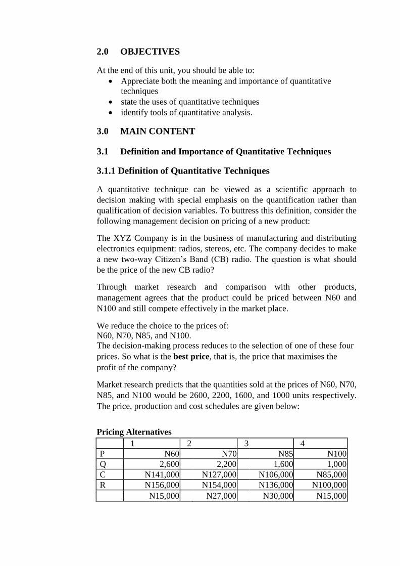
Market research predicts that the quantities sold at the prices of N60, N70,

N85, and N100 would be 2600, 2200, 1600, and 1000 units respectively.

The price, production and cost schedules are given below:

Pricing Alternatives

1 2 3 4

P N60 N70 N85 N100

Q 2,600 2,200 1,600 1,000

C N141,000 N127,000 N106,000 N85,000

R N156,000 N154,000 N136,000 N100,000

N15,000 N27,000 N30,000 N15,000

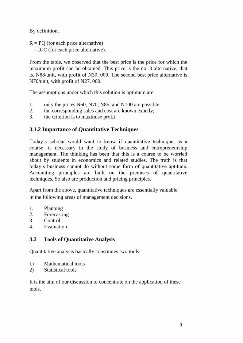
By definition,

R = PQ (for each price alternative)

= R-C (for each price alternative).

From the table, we observed that the best price is the price for which the

maximum profit can be obtained. This price is the no. 3 alternative, that

is, N88/unit, with profit of N30, 000. The second best price alternative is

N70/unit, with profit of N27, 000.

The assumptions under which this solution is optimum are:

1. only the prices N60, N70, N85, and N100 are possible; 2. the corresponding sales and cost are known exactly; 3. the criterion is to maximise profit.

3.1.2 Importance of Quantitative Techniques

Today’s scholar would want to know if quantitative technique, as a

course, is necessary in the study of business and entrepreneurship

management. The thinking has been that this is a course to be worried

about by students in economics and related studies. The truth is that

today’s business cannot do without some form of quantitative aptitude.

Accounting principles are built on the premises of quantitative

techniques. So also are production and pricing principles.

Apart from the above, quantitative techniques are essentially valuable

in the following areas of management decisions.

1. Planning 2. Forecasting

3. Control 4. Evaluation

3.2 Tools of Quantitative Analysis

Quantitative analysis basically constitutes two tools.

1) Mathematical tools 2) Statistical tools

It is the aim of our discussion to concentrate on the application of these

tools.

9

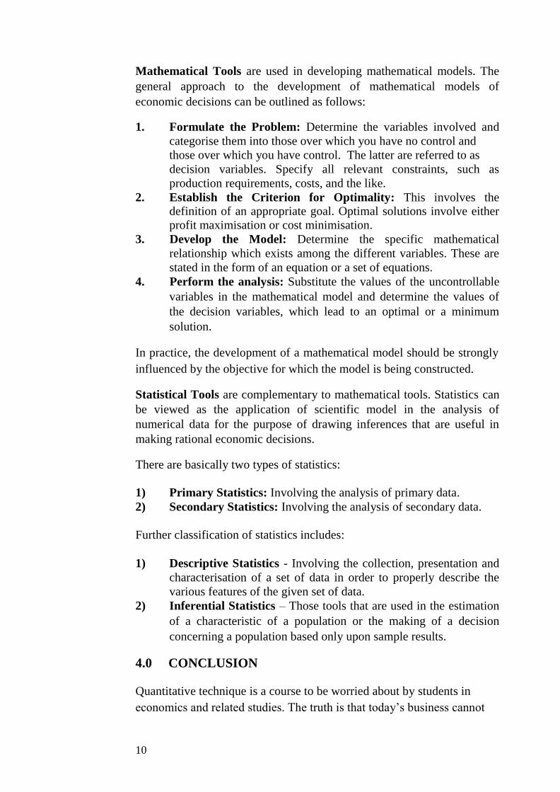
Mathematical Tools are used in developing mathematical models. The

general approach to the development of mathematical models of

economic decisions can be outlined as follows:

1. Formulate the Problem: Determine the variables involved and

categorise them into those over which you have no control and

those over which you have control. The latter are referred to as

decision variables. Specify all relevant constraints, such as

production requirements, costs, and the like.

2. Establish the Criterion for Optimality: This involves the

definition of an appropriate goal. Optimal solutions involve either

profit maximisation or cost minimisation. 3. Develop the Model: Determine the specific mathematical

relationship which exists among the different variables. These are

stated in the form of an equation or a set of equations.

4. Perform the analysis: Substitute the values of the uncontrollable

variables in the mathematical model and determine the values of

the decision variables, which lead to an optimal or a minimum

solution.

In practice, the development of a mathematical model should be strongly

influenced by the objective for which the model is being constructed.

Statistical Tools are complementary to mathematical tools. Statistics can

be viewed as the application of scientific model in the analysis of

numerical data for the purpose of drawing inferences that are useful in

making rational economic decisions.

There are basically two types of statistics:

1) Primary Statistics: Involving the analysis of primary data. 2) Secondary Statistics: Involving the analysis of secondary data.

Further classification of statistics includes:

1) Descriptive Statistics - Involving the collection, presentation and

characterisation of a set of data in order to properly describe the

various features of the given set of data. 2) Inferential Statistics – Those tools that are used in the estimation

of a characteristic of a population or the making of a decision

concerning a population based only upon sample results.

4.0 CONCLUSION

Quantitative technique is a course to be worried about by students in

economics and related studies. The truth is that today’s business cannot

10

do without some form of quantitative aptitude. Accounting principles

are built on the premises of quantitative techniques. So also are

production and pricing principles.

Apart from the above, quantitative techniques are essentially valuable

in the following areas of management decisions.

1. Planning 2. Forecasting

3. Control 4. Evaluation

5.0 SUMMARY

This unit provided some background information on the study of

quantitative methods. In a nutshell, the followings were the major

information obtained from the discussions.

1. A quantitative technique can be viewed as a scientific approach to

decision making with special emphasis on the quantification rather

than qualification of decision variables. 2. Quantitative analysis basically constitutes two tools:

Mathematical tools

Statistical tools

3. The development of a mathematical model should be strongly

influenced by the objective for which the model is being

constructed. Statistical tools are complementary to mathematical

tools. Statistics in general, can be viewed as the application of

scientific model, in the analysis of numerical data, for the purpose

of drawing inferences that are useful in making rational economic

decisions.

6.0 TUTOR-MARKED ASSIGNMENT

7.0 REFERENCES/FURTHER READING

Haessuler, E. F. and Paul, R. S. (1976). Introductory Mathematical

Analysis for Students of Business and Economics, (2nd

edition.)

Reston Virginia: Reston Publishing Company.

11

UNIT 2 MATHEMATICAL TOOLS I: EQUATIONS

AND INEQUALITIES

CONTENTS

1.0 Introduction

2.0 Objectives

3.0 Main Content

3.1 Linear Equations

3.2 Quadratic Equations

3.3.1 Solving By Factorisation

3.3.2 Solving by the Quadratic Formula

4.0 Conclusion

5.0 Summary



1.0 INTRODUCTION

An Equation is a mathematical model expressing the relationship between

variables. An Inequality, on the other hand, expresses the differences

among variables.

Although there are several types of equations and inequalities, depending

on the degree of relationship, our major concern here is on Linear and

Quadratic Equations, as well as Linear Inequalities.

2.0 OBJECTIVES


explain what mathematical equations are all about and how to

formulate them

state the business applications of linear and quadratic equations

recognise the linear equations that are applicable to business

decisions

formulate equations for the solution of simple decision problems.

3.0 MAIN CONTENT

3.1 Linear Equations and Quadratic Equations

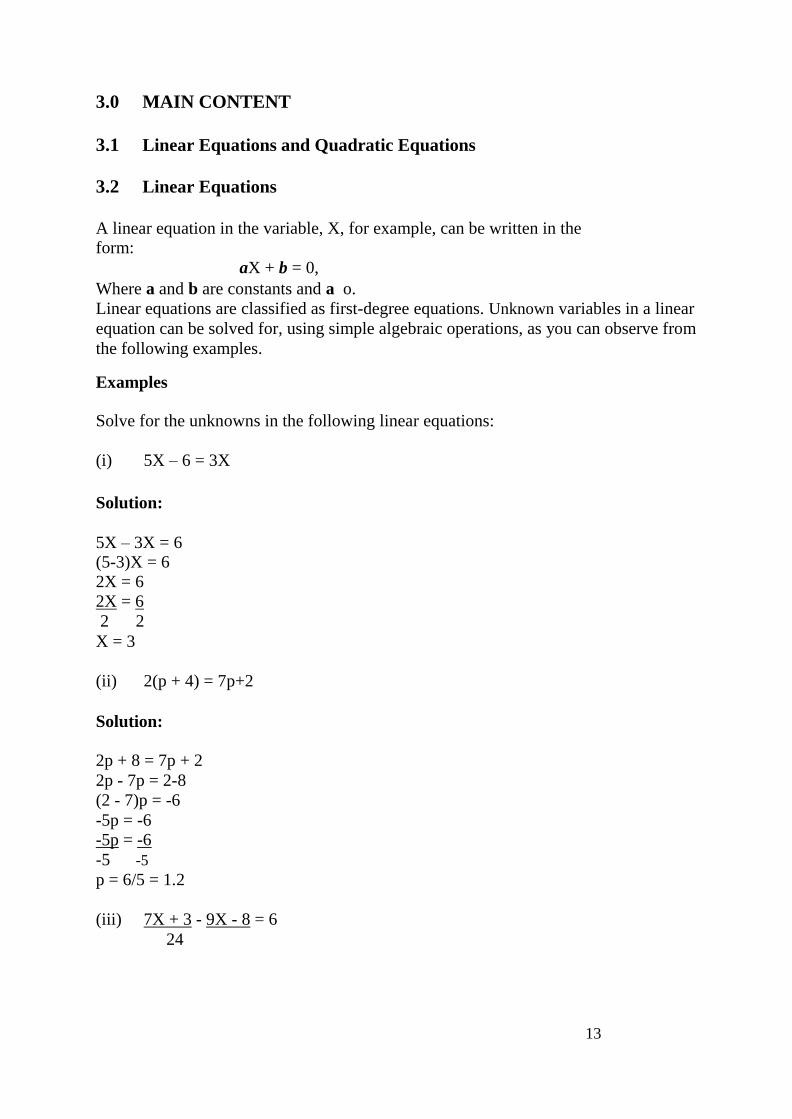
3.2 Linear Equations

A linear equation in the variable, X, for example, can be written in the form:

aX + b = 0,

Where a and b are constants and a o.

Linear equations are classified as first-degree equations. Unknown variables in a linear

equation can be solved for, using simple algebraic operations, as you can observe from

the following examples.

Examples

Solve for the unknowns in the following linear equations:

(i) 5X – 6 = 3X

Solution:

5X – 3X = 6 (5-3)X = 6

2X = 6

2X = 6

2 2 X = 3

(ii) 2(p + 4) = 7p+2

Solution:

2p + 8 = 7p + 2

2p - 7p = 2-8

(2 - 7)p = -6

-5p = -6

-5p = -6

-5 -5

p = 6/5 = 1.2

(iii) 7X + 3 - 9X - 8 = 6 24

13

Solution:

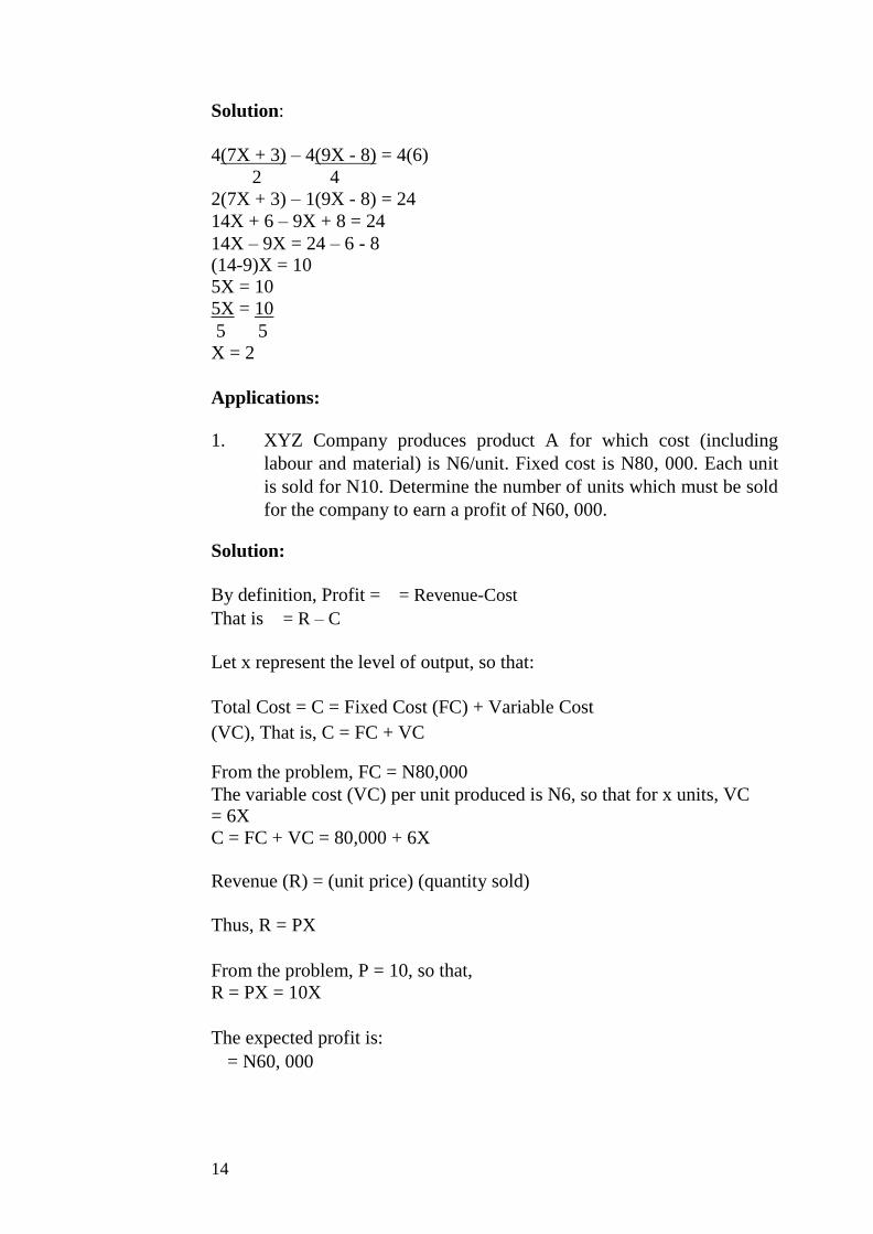
4(7X + 3) – 4(9X - 8) = 4(6)

2 4

2(7X + 3) – 1(9X - 8) = 24

14X + 6 – 9X + 8 = 24

14X – 9X = 24 – 6 - 8 (14-9)X = 10

5X = 10

5X = 10

5 5

X = 2

Applications:

1. XYZ Company produces product A for which cost (including

labour and material) is N6/unit. Fixed cost is N80, 000. Each unit

is sold for N10. Determine the number of units which must be sold

for the company to earn a profit of N60, 000.

Solution:

By definition, Profit = = Revenue-Cost

That is = R – C

Let x represent the level of output, so that:

Total Cost = C = Fixed Cost (FC) + Variable Cost

(VC), That is, C = FC + VC

From the problem, FC = N80,000

The variable cost (VC) per unit produced is N6, so that for x units, VC = 6X

C = FC + VC = 80,000 + 6X

Revenue (R) = (unit price) (quantity sold)

Thus, R = PX

From the problem, P = 10, so that,

R = PX = 10X

The expected profit is:

= N60, 000

14

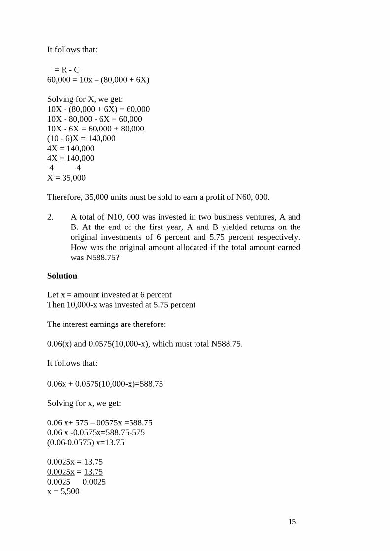
It follows that:

= R - C

60,000 = 10x – (80,000 + 6X)

Solving for X, we get:

10X - (80,000 + 6X) = 60,000

10X - 80,000 - 6X = 60,000

10X - 6X = 60,000 + 80,000

(10 - 6)X = 140,000

4X = 140,000 4X = 140,000

4 4 X = 35,000

Therefore, 35,000 units must be sold to earn a profit of N60, 000.

2. A total of N10, 000 was invested in two business ventures, A and

B. At the end of the first year, A and B yielded returns on the

original investments of 6 percent and 5.75 percent respectively.

How was the original amount allocated if the total amount earned

was N588.75?

Solution

Let x = amount invested at 6 percent

Then 10,000-x was invested at 5.75 percent

The interest earnings are therefore:

0.06(x) and 0.0575(10,000-x), which must total N588.75.

It follows that:

0.06x + 0.0575(10,000-x)=588.75

Solving for x, we get:

0.06 x+ 575 – 00575x =588.75

0.06 x -0.0575x=588.75-575

(0.06-0.0575) x=13.75

0.0025x = 13.75

0.0025x = 13.75

0.0025 0.0025

x = 5,500

15

Thus, N5, 500 was invested at 6 percent, while N (10,000-5,500) = N4,

500 was invested at 5.75 percent.

3.2 Quadratic Equations

A Quadratic Equation is an equation of the second degree. It is of the

form:

aX2 + bX + c=0,

Where a, b, and c are constants.

There are two basic methods of solving quadratic equations:

(1) By Factorisation

(2) By the use of Quadratic formula.

3.2.1 Solving By Factorisation

This involves the determination of the factors that form the given

quadratic equation. This will then make the solutions for the unknown

easy to come by, as you can see from the following examples.

Examples

(1) Solve for x in the quadratic

equation: X2 + X – 12 = 0

Factorising the left hand side, we get:

X - 3

X

+ 4

(X – 3) and (X + 4) are the factors, so that

(X - 3)(X+ 4) = 0

For this equation to hold, either X – 3 = 0 or X+ 4 = 0

It follows that:

If X – 3 = 0

then, X = 3 and if X + 4 = 0

then, X = -4

16

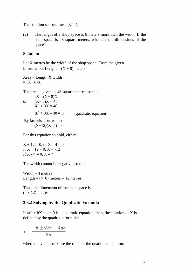
The solution set becomes: [3, - 4]

(2) The length of a shop space is 8 meters more than the width. If the

shop space is 48 square meters, what are the dimensions of the

space?

Solution:

Let X metres be the width of the shop space. From the given

information, Length = (X + 8) meters.

Area = Length X width

= (X+ 8)X

The area is given as 48 square metres, so that:

48 = (X+ 8)X

or (X+ 8)X = 48

X2 + 8X = 48

X2 + 8X – 48 = 0 (quadratic equation)

By factorisation, we get:

(X+12)(X- 4) = 0

For this equation to hold, either

X + 12 = 0, or X – 4 = 0

If X + 12 = 0, X = -12

If X - 4 = 0, X = 4

The width cannot be negative, so that

Width = 4 metres

Length = (4+8) metres = 12 metres.

Thus, the dimension of the shop space is

(4 x 12) metres.

3.3.2 Solving by the Quadratic Formula

If ax2 + bX + c = 0 is a quadratic equation, then, the solution of X is

defined by the quadratic formula:

where the values of x are the roots of the quadratic equation.

17

Examples:

(1) Solve for x in:

4x2 -17x+15 = 0

Solution:

Using the quadratic formula, a = 4; b = -17; c = 15. By substitution to

the formula, we get:

= 17 ±7

8

X = 17+7 or X = 17-7

8 8

X = 3 or X = 1.25

18

Application:

1. The board of directors of Chizy Co. Ltd. agrees to redeem some of

its bonds in 2 years. At that time, N1, 102,500 will be required for

the redemption. Let us suppose N1, 000,000 is presently set aside.

At what compound annual rate of interest will the N1, 000,000

have to be invested in order that its future value will be sufficient

to redeem the bonds?

Solution:

Let r = annual rate of interest

At the end of the first year, the accumulated amount will be:

N1, 000,000 + the interest on it

= 1,000,000 + 1,000,000 (r)

= 1,000,000 (1+r)

Since the interest is compounded, at the end of the second year, the

accumulated amount would be:

1,000,000 (1+r)+interest on it:

1,000,000 (1+r)+1,000,000 (1+r)r

According to the problem, the total value at the end of the second year

is:

1,000,000 (1+r)+1,000,000 (1+r)r = 1,102,500

Solving for r, we get:

1,000,000 (1+r)+1,000,000(1+r)r=1,102,500

1,000,000 [(1+r)+(1+r)r] = 1,102,500

1,000,000 [1+r+r+r2] = 1,202,500

1,000,000 (r2+2r+1)=1,102,500

1,000,000 (1+r)(1+r)=1,102,500 1,000,000 (1+r)

2=1,102,500

(1+r)2 =

=1.103

1+r =± 1.103

r = -1± 1.103 = -1±1.03

r=-1+1.03 or 1+r = -1-1.03

r = 0.103 or r = 2.103

19

Interest rate cannot be negative, therefore, the desired rate of interest is

- .05 or 5 percent.

SELF ASSESSMENT EXERCISE 1

A company produces product X at a unit cost of N10. If fixed costs are

N450, 000, and each unit sells for N25, how many must be sold for the

company to make a positive profit of N510,000.

4.0 CONCLUSION

You have been acquainted with the concepts of equalities and

inequalities, how they can be formulated, solved and applied to practical

business decisions. Specifically, two types of equations were discussed,

these are linear equations and quadratic equations. You must also have

been exposed to the two basic methods of solving quadratic equations: the

use of factors; and, the use of quadratic formula.

5.0 SUMMARY

1. Linear equations are classified as first-degree equations.

Unknown variables in a linear equation can be solved for, using

simple algebraic operations.

2. A quadratic equation is an equation of the second degree. It is of the form:

aX2 + bX + c=0,

where a, b, and c are constants.

There are two basic methods of solving quadratic equations:

(i) By factorisation

(ii) By use of the quadratic formula


To produce 1 unit of a new product, a company determines that the cost

for material is N2.50 per unit and the cost of labour is N4 per unit. The

constant overhead cost is N5, 000. If the cost to a wholesaler is N7.50 per

unit, determine the least number of units that must be sold by the

company to realise a positive profit.




edition.)


20

UNIT 3 MATHEMATICAL TOOLS I (CONTINUED):

SIMULTANEOUS EQUATIONS, LINEAR

FUNCTIONS, AND LINEAR INEQUALITIES

CONTENTS

1.0 Introduction

2.0 Objectives

3.0 Main Content

3.1 Simultaneous Equations

3.2 Linear Functions

3.3 Linear Inequalities

4.0 Conclusion

5.0 Summary



1.0 INTRODUCTION

This unit is a continuation of our discussions on mathematical tools. This

focuses on the other aspects of equations and inequalities that are useful

in business and economic decisions.

2.0 OBJECTIVES


explain what simultaneous equation systems are all about

describe how simultaneous equation systems are formulated and solved

analyse business conditions using linear functions and linear inequalities.

3.0 MAIN CONTENT

3.1 Simultaneous Equations

A simultaneous equation system is a set of equations with two or more

unknown. The mostly used method of solving a simultaneous equation

system is the so-called “Addition-Subtraction” or “Elimination” method.

Consider the following example:

Solve for X and Y in the system of equations:

21

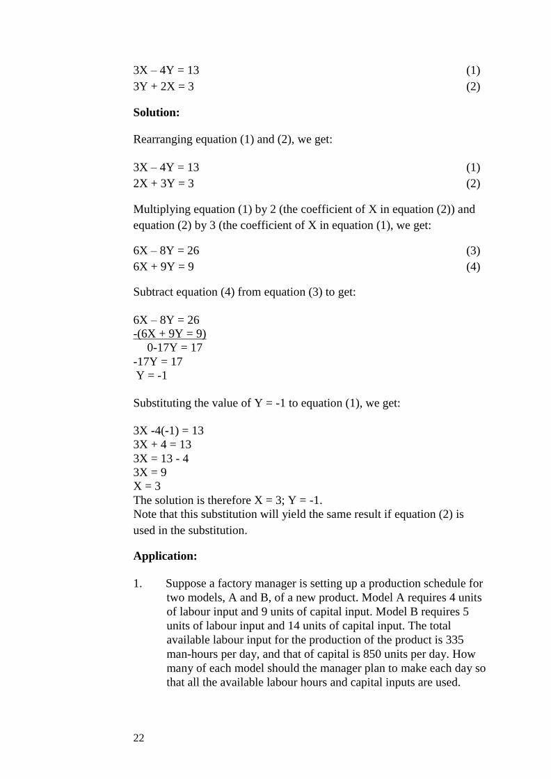
3X – 4Y = 13 (1)

3Y + 2X = 3 (2)

Solution:

Rearranging equation (1) and (2), we get:

3X – 4Y = 13 (1)

2X + 3Y = 3 (2)

Multiplying equation (1) by 2 (the coefficient of X in equation (2)) and

equation (2) by 3 (the coefficient of X in equation (1), we get:

6X – 8Y = 26 (3)

6X + 9Y = 9 (4)

Subtract equation (4) from equation (3) to get:

6X – 8Y = 26

-(6X + 9Y = 9)

0-17Y = 17

-17Y = 17

Y = -1

Substituting the value of Y = -1 to equation (1), we get:

3X -4(-1) = 13

3X + 4 = 13

3X = 13 - 4

3X = 9

X = 3

The solution is therefore X = 3; Y = -1.

Note that this substitution will yield the same result if equation (2) is

used in the substitution.

Application:

1. Suppose a factory manager is setting up a production schedule for

two models, A and B, of a new product. Model A requires 4 units

of labour input and 9 units of capital input. Model B requires 5

units of labour input and 14 units of capital input. The total

available labour input for the production of the product is 335

man-hours per day, and that of capital is 850 units per day. How

many of each model should the manager plan to make each day so

that all the available labour hours and capital inputs are used.

22

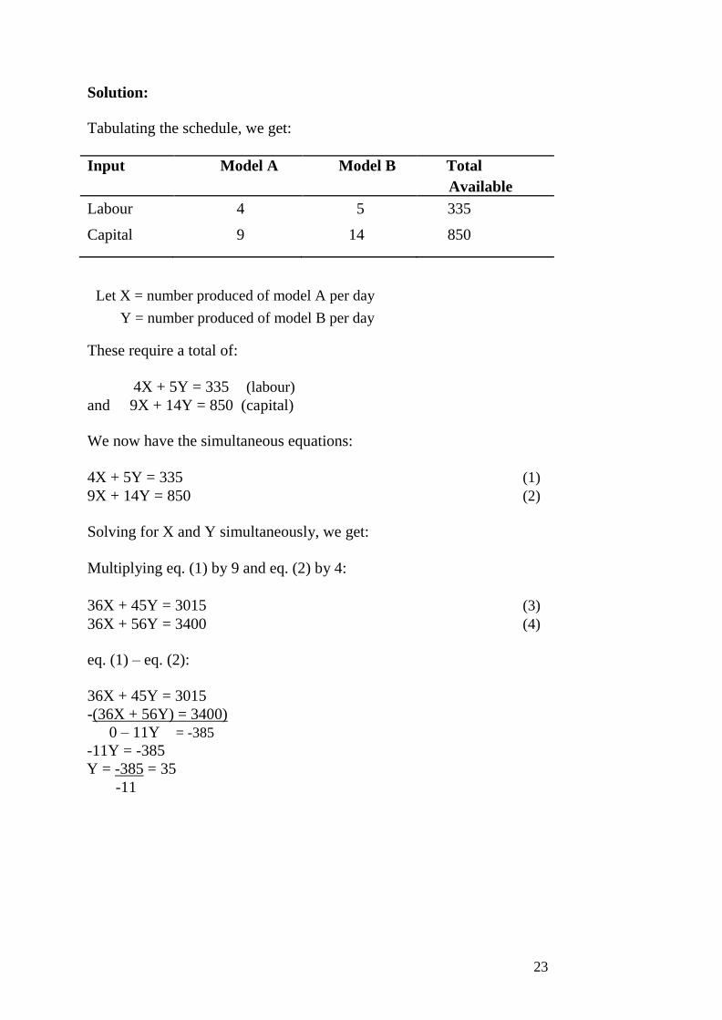
Solution:

Tabulating the schedule, we get:

Input Model A Model B Total

Available

Labour 4 5 335

Capital 9 14 850

Let X = number produced of model A per day

Y = number produced of model B per day

These require a total of:

4X + 5Y = 335 (labour)

and 9X + 14Y = 850 (capital)

We now have the simultaneous equations:

4X + 5Y = 335 (1)

9X + 14Y = 850 (2)

Solving for X and Y simultaneously, we get:

Multiplying eq. (1) by 9 and eq. (2) by 4:

36X + 45Y = 3015 (3)

36X + 56Y = 3400 (4)

eq. (1) – eq. (2):

36X + 45Y = 3015

-(36X + 56Y) = 3400)

0 – 11Y = -385

-11Y = -385

Y = -385 = 35

-11

23

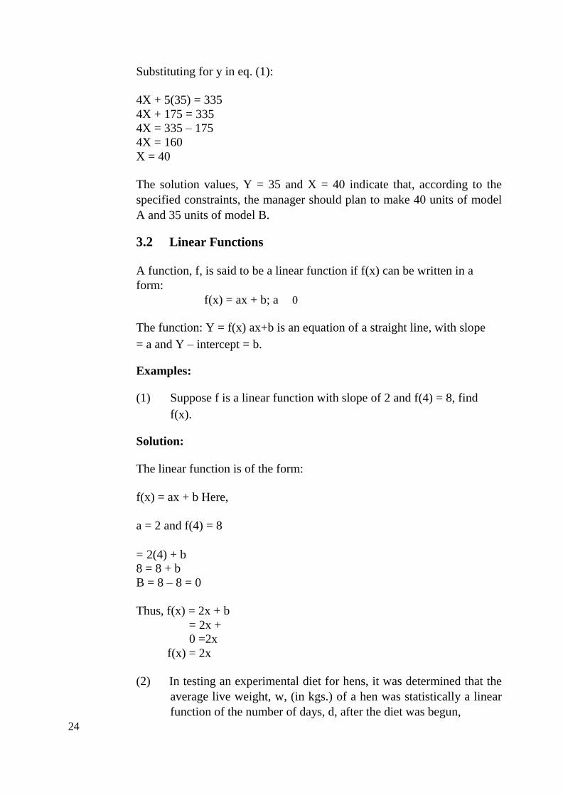
Substituting for y in eq. (1):

4X + 5(35) = 335

4X + 175 = 335

4X = 335 – 175

4X = 160

X = 40

The solution values, Y = 35 and X = 40 indicate that, according to the

specified constraints, the manager should plan to make 40 units of model

A and 35 units of model B.

3.2 Linear Functions

A function, f, is said to be a linear function if f(x) can be written in a

form:

f(x) = ax + b; a 0

The function: Y = f(x) ax+b is an equation of a straight line, with slope

= a and Y – intercept = b.

Examples:

(1) Suppose f is a linear function with slope of 2 and f(4) = 8, find

f(x).

Solution:

The linear function is of the form:

f(x) = ax + b Here,

a = 2 and f(4) = 8

= 2(4) + b 8 = 8 + b

B = 8 – 8 = 0

Thus, f(x) = 2x + b

= 2x +

0 =2x

f(x) = 2x

(2) In testing an experimental diet for hens, it was determined that the

average live weight, w, (in kgs.) of a hen was statistically a linear

function of the number of days, d, after the diet was begun,

24

where 0 δ d δ 50. Suppose the average weight of a hen beginning

the diet was 4kg. And 25 days later, it was 7kg.

a) Determine w as a linear function of d. b) What is the average weight of a hen for a 10 days period?

Solutions

a) The required function is of the

form: W = f(d) = md + b,

W = f(d) = b x md

Where w = weight

b = y intercept

m = slope

d = number of days

f(d) = 4kg = b + m x o …. Eqtn 1

at the beginning d = o

w = 4kg

25 days later the weight = 7kg

Therefore we have:

7kg = b + m x 25 … Eqtn 2

Where w = 7kg

d = 25

from eqtn (1) we have

4kg = b + m x o

:. b = 4kg

Substitute b in equation (2) we have 7 = 4 + 25m

7 – 4 = 25m; m = 3/25 = 0.12

Therefore the linear function can be written as

(a) f(d) = 4 + 0.12d = w

(b) d = 10 days; therefore the average weight after 10 days is f(d) = 4 + 0.12 x 10 =

4 + 1.2 = 5.2kg

3.3 Linear Inequalities

An Inequality is simply a statement that two numbers are not equal. A

linear inequality in the variable, X, is an inequality that can be written in

the form:

25

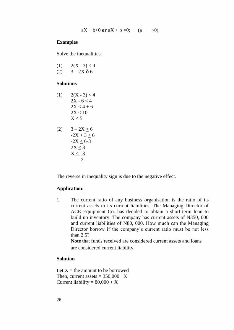
aX + b<0 or aX + b >0; (a >0).

Examples

Solve the inequalities:

(1) 2(X - 3) < 4 (2) 3 – 2X δ 6

Solutions

(1) 2(X - 3) < 4

2X - 6 < 4

2X < 4 + 6

2X < 10

X < 5

(2) 3 – 2X < 6

-2X + 3 < 6

-2X < 6-3

2X < 3

X < 3

2

The reverse in inequality sign is due to the negative effect.

Application:

1. The current ratio of any business organisation is the ratio of its

current assets to its current liabilities. The Managing Director of

ACE Equipment Co. has decided to obtain a short-term loan to

build up inventory. The company has current assets of N350, 000

and current liabilities of N80, 000. How much can the Managing

Director borrow if the company’s current ratio must be not less

than 2.5? Note that funds received are considered current assets and loans

are considered current liability.

Solution

Let X = the amount to be borrowed

Then, current assets = 350,000 +X

Current liability = 80,000 + X

26

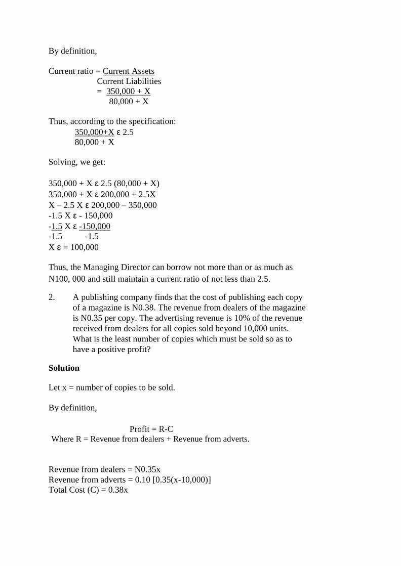
By definition,

Current ratio = Current Assets

Current Liabilities

= 350,000 + X 80,000 + X

Thus, according to the specification:

350,000+X ε 2.5

80,000 + X

Solving, we get:

350,000 + X ε 2.5 (80,000 + X)

350,000 + X ε 200,000 + 2.5X

X – 2.5 X ε 200,000 – 350,000

-1.5 X ε - 150,000

-1.5 X ε -150,000

-1.5 -1.5

X ɛ = 100,000

Thus, the Managing Director can borrow not more than or as much as

N100, 000 and still maintain a current ratio of not less than 2.5.

2. A publishing company finds that the cost of publishing each copy

of a magazine is N0.38. The revenue from dealers of the magazine

is N0.35 per copy. The advertising revenue is 10% of the revenue

received from dealers for all copies sold beyond 10,000 units.

What is the least number of copies which must be sold so as to

have a positive profit?

Solution

Let x = number of copies to be sold.

By definition,

Profit = R-C Where R = Revenue from dealers + Revenue from adverts.

Revenue from dealers = N0.35x

Revenue from adverts = 0.10 [0.35(x-10,000)]

Total Cost (C) = 0.38x

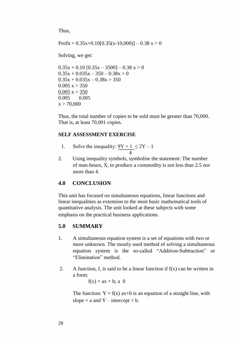
Thus,

Profit = 0.35x+0.10[0.35(x-10,000)] – 0.38 x > 0

Solving, we get:

0.35x + 0.10 [0.35x – 3500] – 0.38 x > 0

0.35x + 0.035x – 350 – 0.38x > 0

0.35x + 0.035x – 0.38x > 350

0.005 x > 350

0.005 x > 350

0.005 0.005

x > 70,000

Thus, the total number of copies to be sold must be greater than 70,000.

That is, at least 70,001 copies.

SELF ASSESSMENT EXERCISE

1. Solve the inequality: 9Y + 1 ≤ 2Y – 1

4

2. Using inequality symbols, symbolise the statement: The number

of man-hours, X, to produce a commodity is not less than 2.5 nor

more than 4.

4.0 CONCLUSION

This unit has focused on simultaneous equations, linear functions and

linear inequalities as extension to the most basic mathematical tools of

quantitative analysis. The unit looked at these subjects with some

emphasis on the practical business applications.

5.0 SUMMARY

1. A simultaneous equation system is a set of equations with two or

more unknown. The mostly used method of solving a simultaneous

equation system is the so-called “Addition-Subtraction” or

“Elimination” method.

2. A function, f, is said to be a linear function if f(x) can be written in

a form:

f(x) = ax + b; a 0

The function: Y = f(x) ax+b is an equation of a straight line, with

slope = a and Y – intercept = b.

28

3. An inequality is simply a statement that two numbers are not equal.

A linear inequality in the variable, X, is an inequality that can be

written in the form:

aX + b<0 or aX + b > 0; (a > 0).


Let P = 0.09q + 50 be the supply equation for a manufacturer. The

demand equation for his product is:

P = 0.07q + 65

a) If a tax of N1.50/unit is to be imposed on the manufacturer, how

will the original equilibrium price be effected if the demand

remains the same? b) Determine the total revenue obtained by the manufacturer at the

equilibrium point, both before and after the tax.




edition.)


29

UNIT 4 MAHEMATICAL TOOLS II: INTRODUCTION

TO MATRIX ALGEBRA

CONTENTS

1.0 Introduction.

2.0 Objectives

3.0 Main Content

3.1 Equality of Matrices

3.2 Matrix Addition

3.3 Scalar Multiplication

3.4 Matrix Multiplication

4.0 Conclusion

5.0 Summary



1.0 INTRODUCTION

An understanding of matrices and their operations is essential for input

output analysis in business and economic decisions. It is also essential for

solving complicated problems in simultaneous equation systems. In this

unit, you will just be introduced to the basic rudimentary of matrices, with

some simple applications.

A matrix is a rectangular array of numbers, called entries. Examples are:

2.0 OBJECTIVES


state the basic principles of matrix algebra

analyse the important mathematical operations of

matrices apply matrices in business decisions.

30

3.0 MAIN CONTENT

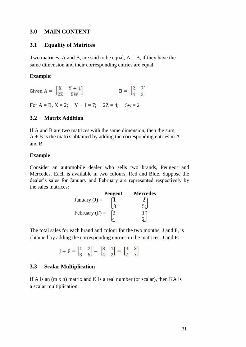
3.1 Equality of Matrices

Two matrices, A and B, are said to be equal, A = B, if they have the

same dimension and their corresponding entries are equal.

Example:

For A = B, X = 2; Y + 1 = 7; 2Z = 4; 5w = 2

3.2 Matrix Addition

If A and B are two matrices with the same dimension, then the sum,

A + B is the matrix obtained by adding the corresponding entries in A

and B.

Example

Consider an automobile dealer who sells two brands, Peugeot and

Mercedes. Each is available in two colours, Red and Blue. Suppose the

dealer’s sales for January and February are represented respectively by

the sales matrices:

Peugeot Mercedes

January (J) = 1 2

3 5;

February (F) = 3 1

4 2

The total sales for each brand and colour for the two months, J and F, is

obtained by adding the corresponding entries in the matrices, J and F:

3.3 Scalar Multiplication

If A is an (m x n) matrix and K is a real number (or scalar), then KA is

a scalar multiplication.

31

Example

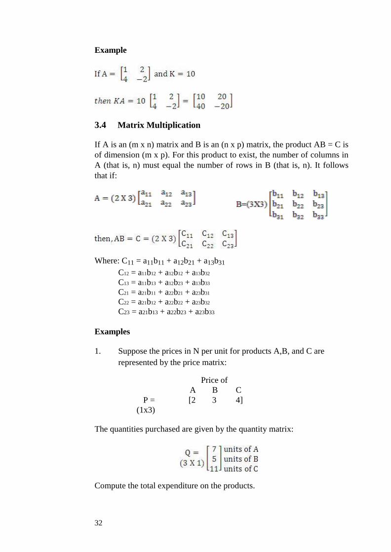
3.4 Matrix Multiplication

If A is an (m x n) matrix and B is an (n x p) matrix, the product AB = C is

of dimension (m x p). For this product to exist, the number of columns in

A (that is, n) must equal the number of rows in B (that is, n). It follows

that if:

Where: C11 = a11b11 + a12b21 + a13b31

C12 = a11b12 + a12b12 + a13b32

C13 = a11b13 + a12b23 + a13b33

C21 = a21b11 + a22b21 + a23b31

C22 = a21b12 + a22b22 + a23b32

C23 = a21b13 + a22b23 + a23b33

Examples

1. Suppose the prices in N per unit for products A,B, and C are

represented by the price matrix:

Price of

A B C

P = [2 3 4]

(1x3)

The quantities purchased are given by the quantity matrix:

Compute the total expenditure on the products.

32

Solution

Required to compute PQ:

= 2(7) + 3(5) + 4(11) = [ 73 ]

(1x1)

Thus, the total expenditure on products A,B, and C is N73.

2. A manufacturer of calculators has an East Coast and a West Coast

plant, each of which produces Business Calculators and Standard

Calculators. The manufacturing time requirements (in hours per

calculator) and the assembly and packaging costs (in naira per

hour) are given by the following matrices:

Hours per Unit

Assembly Packaging

T = 0.2 0.1 Business Calculators

0.2 0.1 Standard Calculators

Naira per Hour

East Coast West Coast

C = 5 6 Assembly

4 5 Packaging

a) What is the total cost of manufacturing a business

calculator on the East Coast?

b) Calculate the manufacturer’s total cost of producing the

calculators in the two plant locations.

Solutions

Question (a) and (b) requires the product matrix:

Where D11 = 0.2(5) + 0.1(4) = 1.4

D12 = 0.2(6) + 0.1(5) = 1.7

D21 = 0.3(5) + 0.1(4) = 1.9

D22 = 0.3(6) + 0.1(5) = 2.3

33

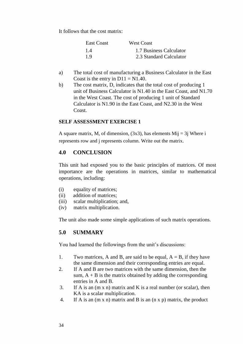
It follows that the cost matrix:

East Coast West Coast

1.4 1.7 Business Calculator

1.9 2.3 Standard Calculator

a) The total cost of manufacturing a Business Calculator in the East

Coast is the entry in D11 = N1.40. b) The cost matrix, D, indicates that the total cost of producing 1

unit of Business Calculator is N1.40 in the East Coast, and N1.70

in the West Coast. The cost of producing 1 unit of Standard

Calculator is N1.90 in the East Coast, and N2.30 in the West

Coast.


A square matrix, M, of dimension, (3x3), has elements Mij = 3j Where i

represents row and j represents column. Write out the matrix.

4.0 CONCLUSION

This unit had exposed you to the basic principles of matrices. Of most

importance are the operations in matrices, similar to mathematical

operations, including:

(i) equality of matrices; (ii) addition of matrices; (iii) scalar multiplication; and, (iv) matrix multiplication.

The unit also made some simple applications of such matrix operations.

5.0 SUMMARY

You had learned the followings from the unit’s discussions:

1. Two matrices, A and B, are said to be equal, A = B, if they have the same dimension and their corresponding entries are equal.

2. If A and B are two matrices with the same dimension, then the

sum, A + B is the matrix obtained by adding the corresponding

entries in A and B. 3. If A is an (m x n) matrix and K is a real number (or scalar), then

KA is a scalar multiplication. 4. If A is an (m x n) matrix and B is an (n x p) matrix, the product

34

AB = C is of dimension (m x p). For this product to exist, the

number of columns in A (that is, n) must equal the number of rows

in B (that is, n).


Suppose a building contractor has accepted orders for five ranch style

houses, seven cape cod-style houses and twelve colonial-style houses.

These orders can be represented by the row matrix

Q = [5 7 12]

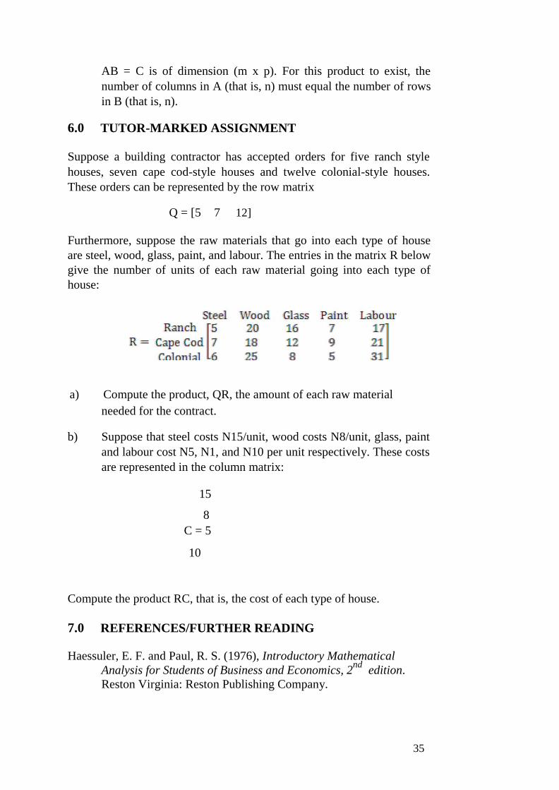
Furthermore, suppose the raw materials that go into each type of house

are steel, wood, glass, paint, and labour. The entries in the matrix R below

give the number of units of each raw material going into each type of

house:

a) Compute the product, QR, the amount of each raw material

needed for the contract. b) Suppose that steel costs N15/unit, wood costs N8/unit, glass, paint

and labour cost N5, N1, and N10 per unit respectively. These costs

are represented in the column matrix:

15

8

C = 5

10

Compute the product RC, that is, the cost of each type of house.


Haessuler, E. F. and Paul, R. S. (1976), Introductory Mathematical

Analysis for Students of Business and Economics, 2nd

edition.


35

UNIT 5 MATHEMATICAL TOOL III: APPLIED

DIFFERENTIAL

CALCULUS CONTENTS

1.0 Introduction

2.0 Objectives

3.0 Main Content

3.1 Derivatives and Rules of Differentiation

3.1.1 Derivatives

3.1.2 Rules of Differentiation

3.2 Applications of Derivatives.

3.2.1 The Marginal Cost

3.3 Applied Maxima and Minima

4.0 Conclusion

5.0 Summary



1.0 INTRODUCTION

This unit provides some foundations in topics of calculus that are relevant

to students in business and economic decisions. You need to note that the

ideas involved in calculus differ from those of algebra and geometry. One

of the major problems dealt with in calculus is that of finding the rate of

change, of decision variables, such as the rate of change of profit over

time, the rate of change of revenue with respect to changes in product

prices, and the like.

2.0 OBJECTIVES


define ‘derivate’ of function

apply the techniques of finding the derivatives by proper

application of rules

differentiate between the “maxima” and “minima” principles

apply calculus in business and economic decisions.

3.0 MAIN CONTENT

3.1 Derivatives and Rules of Differentiation

3.1.1 Derivatives

For a given function, f, the derivative of f at Xo, denoted by f ' (Xo), is

the limit:

36

If a given function, f, has a derivative at Xo, we say that f is differentiable

at Xo. To find the derivative of f is to differentiate f, and the process of

finding a derivative is called differentiation.

If a function, f (X), has a derivative of f ' (Xo) at Xo, then:

(a) the instantaneous rate of change of f (X) relative to X at Xo is f ' (Xo)

(b) the slope of the curve (or the slope of the tangent line to the

curve),

Y= f (X) at (Xo, f (Xo)) is f ' (Xo)

In general, for a given function f, the derivative of f is the function of f '

(X) given by:

We can refer to the derivative f ' (X) as a function whose output value at

Xo is the slope of the curve, Y = f (X) at (Xo, f (Xo)) or the instantaneous

rate of change in f (X) at X = Xo.

Example

Let f be defined by f (X) = X2.

Then, the derivative is:

= 2X as h 0

The symbol, dy/dx, is used to represent the derivative of a function,

Y = f (X). Thus, if Y = f (X), where f is differentiable, then

dy = f ' (X)

dx

37

3.1.2 Rules of Differentiation

The rules of differentiation give us some efficient shortcuts for

calculating derivatives. It is, therefore, not necessary to use the limit

procedures, as in the example above.

The rules are as follows:

Rule 1 (Constant Rule): This states that the derivative of a constant

function is zero. Thus, if Y = f (X) = C, where C is any constant number,

then

dy/dx = f ' (X) = 0

Rule 2 (Constant Multiplier Rule): If the function f, is differentiable

at X, then so is any constant multiple of f;

Rule 3 (The Power Rule): For any positive integer, n, the function f

(X) = Xn is differentiable everywhere, and

Rule 4 (Sum and Difference Rule): If f (X) and g (X) are both

differentiable at X, then so are f (X) + g (X) and f (X) – g (X). And

Examples

1.

2.

Rule 5 (The Product Rule): If the functions f (X) and g (X) are both

differentiable at X, then so is their product, f (X) g (X). And,

Example

38

= (X5 + 2X

3 – 5)(12X

3 – 4X) + (3X

4 – 2X

2 + 8)(5X

4 + 6X

2)

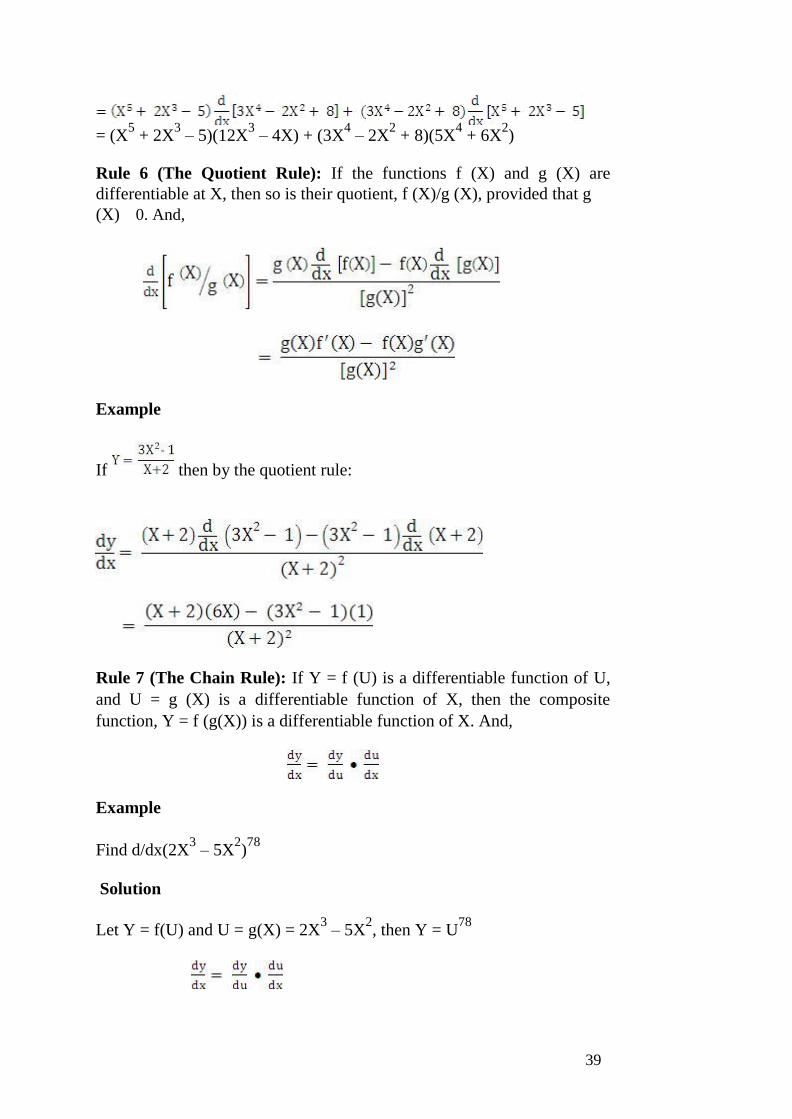
Rule 6 (The Quotient Rule): If the functions f (X) and g (X) are

differentiable at X, then so is their quotient, f (X)/g (X), provided that g

(X) 0. And,

Example

If then by the quotient rule:

Rule 7 (The Chain Rule): If Y = f (U) is a differentiable function of U,

and U = g (X) is a differentiable function of X, then the composite

function, Y = f (g(X)) is a differentiable function of X. And,

Example

Find d/dx(2X3 – 5X

2)78

Solution

Let Y = f(U) and U = g(X) = 2X3 – 5X

2, then Y = U

78

39

= 78(2X3 – 5X

2 )

77 (6X

2 –

10X) (Since U = 2X3 – 5X

2)

3.2 Applications of Derivatives

The following few examples demonstrate the economic applications of

the concept of derivatives.

1. Find the rate of change of the variable Y = X4 with respect to X.

Evaluate the rate when X = 2 and when X= -1.

Solution

By the concepts of derivatives, if Y = X4,

This implies that if X increases by a small amount, then Y will increase

approximately 32 times as much. Or put differently, Y increases 32 times

as fast as X does.

Implying that Y decreases 4 times as fast as X increases.

2. Let P = 100 – q2 represent a demand function. Find the rate of

change of price, P, with respect to unit changes in q. How fast is

the price changing with respect to q, when q = 5, assuming that P

is in naira?

Solution

The rate of change of P with respect to q is:

40

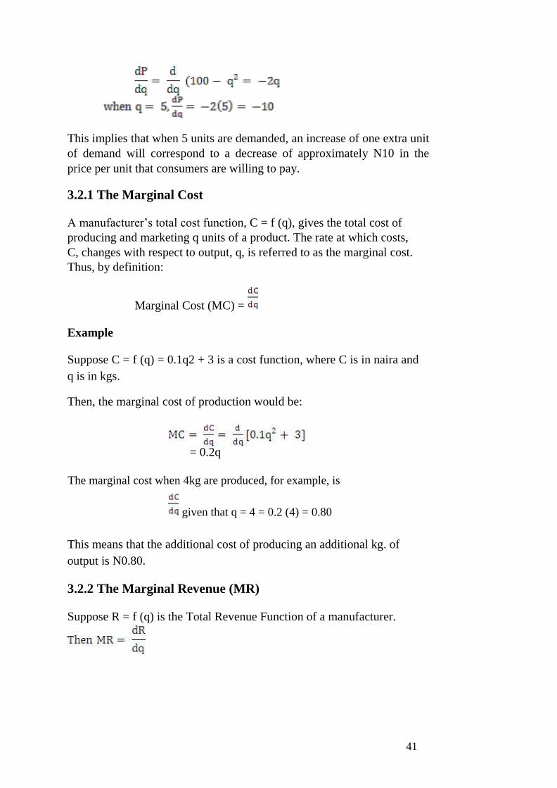
This implies that when 5 units are demanded, an increase of one extra unit

of demand will correspond to a decrease of approximately N10 in the

price per unit that consumers are willing to pay.

3.2.1 The Marginal Cost

A manufacturer’s total cost function, C = f (q), gives the total cost of

producing and marketing q units of a product. The rate at which costs,

C, changes with respect to output, q, is referred to as the marginal cost.

Thus, by definition:

Marginal Cost (MC) =

Example

Suppose C = f (q) = 0.1q2 + 3 is a cost function, where C is in naira and

q is in kgs.

Then, the marginal cost of production would be:

= 0.2q

The marginal cost when 4kg are produced, for example, is

given that q = 4 = 0.2 (4) = 0.80

This means that the additional cost of producing an additional kg. of

output is N0.80.

3.2.2 The Marginal Revenue (MR)

Suppose R = f (q) is the Total Revenue Function of a manufacturer.

41

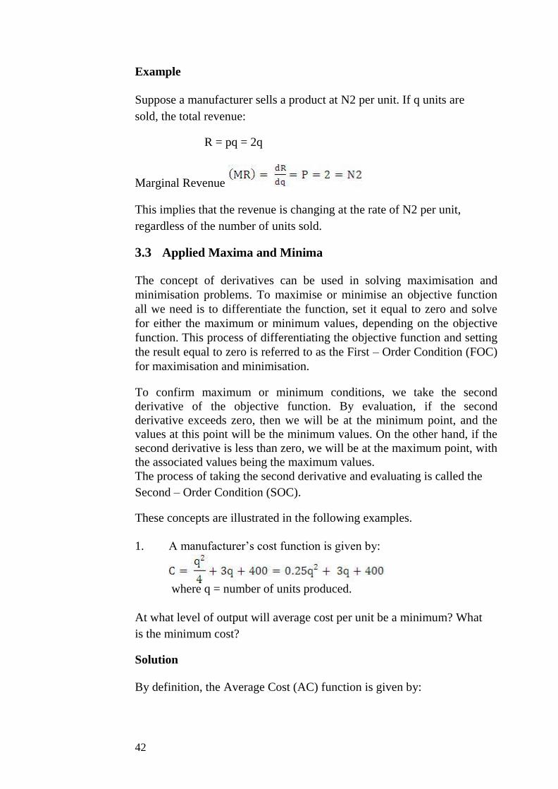
Example

Suppose a manufacturer sells a product at N2 per unit. If q units are

sold, the total revenue:

R = pq = 2q

Marginal Revenue

This implies that the revenue is changing at the rate of N2 per unit,

regardless of the number of units sold.

3.3 Applied Maxima and Minima

The concept of derivatives can be used in solving maximisation and

minimisation problems. To maximise or minimise an objective function

all we need is to differentiate the function, set it equal to zero and solve

for either the maximum or minimum values, depending on the objective

function. This process of differentiating the objective function and setting

the result equal to zero is referred to as the First – Order Condition (FOC)

for maximisation and minimisation.

To confirm maximum or minimum conditions, we take the second

derivative of the objective function. By evaluation, if the second

derivative exceeds zero, then we will be at the minimum point, and the

values at this point will be the minimum values. On the other hand, if the

second derivative is less than zero, we will be at the maximum point, with

the associated values being the maximum values.

The process of taking the second derivative and evaluating is called the

Second – Order Condition (SOC).

These concepts are illustrated in the following examples.

1. A manufacturer’s cost function is given by:

where q = number of units produced.

At what level of output will average cost per unit be a minimum? What

is the minimum cost?

Solution

By definition, the Average Cost (AC) function is given by:

42

= 0.25q + 3 + 400q-1

To minimise the Average Cost, we differentiate to get:

Setting this equal to zero according to the FOC, we get:

0.25 – 400q-2

= 0

0.25q2 = 400

q = ± 1600 = ±40

For q >0, the cost minimising level of output is q = 40 units. Thus, the

level of output for which average cost per unit will be minimum is 40

units.

2. The demand equation for a manufacturer’s product is given by:

P = 80 – X

4

(a) At what value of X will there be a maximum revenue?

(b) What is the maximum revenue?

Solution

By definition, revenue (R) = PX

Thus, R = PX = (20 – 0.25X)X

= 20X – 0.25X2

By the first - order condition:

Setting this equal to zero and solving for X, we get:

20 – 0.5X = 0

43

0.5X = 20

Thus, the value of X which the revenue will be maximised is 40 units.


A Computer Service Bureau generates revenue at the rate R (t) = 20 + 16t

– t2 thousand naira in its t years of operation, while its average cost of

operation is

(a) When is the revenue of the firm greatest and what is its value? (b) For how many years is the operation of the firm profitable?

(c) When is the profit of the firm optimum?

4.0 CONCLUSION

This unit has provided you with some foundations in topics of calculus

that are relevant to students in business and economic decisions. You

need to note that the ideas involved in calculus differ from those of

algebra and geometry. You should also note that the major problems dealt

with in calculus is that of finding the rate of change of decision variables,

such as the rate of change of profit over time, the rate of change of

revenue with respect to changes in product prices, and the like.

You observed from this unit that the concept of derivatives can be used in

solving maximisation and minimisation problems. To maximise or

minimise an objective function all we need is to differentiate the function,

set it equal to zero and solve for either the maximum or minimum values,

depending on the objective function. This process of differentiating the

objective function and setting the result equal to zero is referred to as the

First – Order Condition (FOC) for maximisation and minimisation.

To confirm maximum or minimum conditions, you take the second

derivative of the objective function. By evaluation, if the second

derivative exceeds zero, then we will be at the minimum point, and the

values at this point will be the minimum values. On the other hand, if the

second derivative is less than zero, we will be at the maximum point, with

the associated values being the maximum values.

44

The process of taking the second derivative and evaluating is called the

Second – Order Condition (SOC).

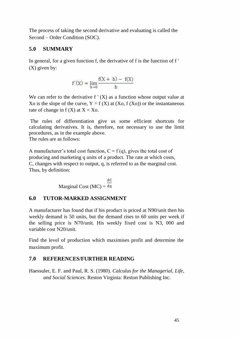
5.0 SUMMARY

In general, for a given function f, the derivative of f is the function of f '

(X) given by:

We can refer to the derivative f ' (X) as a function whose output value at

Xo is the slope of the curve, Y = f (X) at (Xo, f (Xo)) or the instantaneous

rate of change in f (X) at X = Xo.

The rules of differentiation give us some efficient shortcuts for calculating derivatives. It is, therefore, not necessary to use the limit

procedures, as in the example above.

The rules are as follows:

A manufacturer’s total cost function, C = f (q), gives the total cost of

producing and marketing q units of a product. The rate at which costs,

C, changes with respect to output, q, is referred to as the marginal cost.

Thus, by definition:

Marginal Cost (MC) =


A manufacturer has found that if his product is priced at N90/unit then his

weekly demand is 50 units, but the demand rises to 60 units per week if

the selling price is N70/unit. His weekly fixed cost is N3, 000 and

variable cost N20/unit.

Find the level of production which maximises profit and determine the

maximum profit.


Haessuler, E. F. and Paul, R. S. (1980). Calculus for the Managerial, Life,

and Social Sciences. Reston Virginia: Reston Publishing Inc.

45

MODULE 2

Unit 1 Statistical Tool I: Measures of Averages

Unit 2 Statistical Tools II: Measures of Variability or Dispersion

Unit 3 Statistical Tools III: Sets and Set Operations

Unit 4 Statistical Tools IV: Probability Theory and Applications

Unit 5 Correlation Theory

UNIT 1 STATISTICAL TOOLS I: MEASURES OF

AVERAGES

1.0 Introduction

2.0 Objectives

3.0 Main Content

3.1 Arithmetic Mean

3.1.1 Arithmetic Mean for Observations of Equal Weight

3.1.2 Weighted Arithmetic Mean

3.1.3 Arithmetic Mean for a Grouped Data

3.2 The Median

3.2.1 Median for a Grouped Data

3.3 The Mode

3.3.1 Mode for a Grouped Data

4.0 Conclusion

5.0 Summary



1.0 INTRODUCTION

46

Units 1 and 2 will be devoted mainly to the simple statistical tools

needed for business and economic decisions. In this unit, we focus on the

concept of averages. It is essential for any business person to understand

this concept as it forms the basis for the establishment of targets and

yardsticks for measures of success. The units introduce two important

and often used statistical measures in quantitative techniques:

the measure of central tendency

the measure of disper.

2.0 OBJECTIVES


state the importance and measures of central tendency or

averages

state the measures and uses of dispersion or deviations from

averages

apply the principles of averages and dispersion in day-to-day

business decisions.

3.0 MAIN CONTENT

3.1 Measures of Central Tendency or Averages

The three important measures of central tendency to be discussed here,

among others include:

1. arithmetic mean 2. median

3. mode

47

3.2 Arithmetic Mean

The arithmetic mean is used in estimating the average of a given set of

observations. It is the most accurate measure of an average. Of major

concern in the present discussion are three levels of estimates:

arithmetic mean of observations of equal weights or levels of

importance.

arithmetic mean of weighted set of observations (weighted

arithmetic mean)

arithmetic mean for a grouped data (or set of observations)

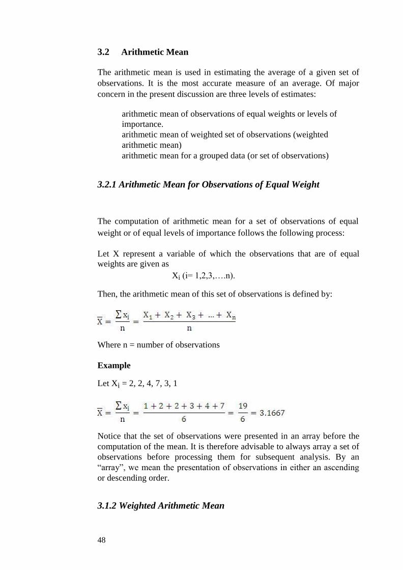
3.2.1 Arithmetic Mean for Observations of Equal Weight

The computation of arithmetic mean for a set of observations of equal

weight or of equal levels of importance follows the following process:

Let X represent a variable of which the observations that are of equal

weights are given as

Xi (i= 1,2,3,….n).

Then, the arithmetic mean of this set of observations is defined by:

Where n = number of observations

Example

Let Xi = 2, 2, 4, 7, 3, 1

Notice that the set of observations were presented in an array before the

computation of the mean. It is therefore advisable to always array a set of

observations before processing them for subsequent analysis. By an

“array”, we mean the presentation of observations in either an ascending

or descending order.

3.1.2 Weighted Arithmetic Mean

48

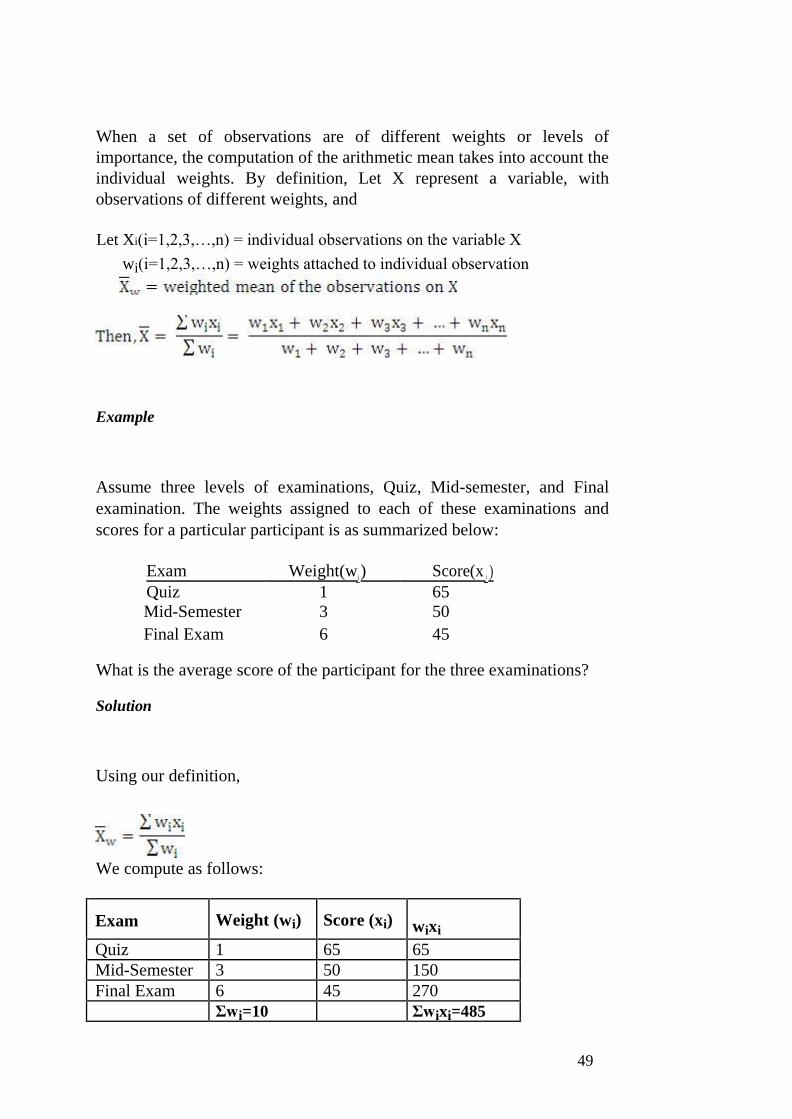
When a set of observations are of different weights or levels of

importance, the computation of the arithmetic mean takes into account the

individual weights. By definition, Let X represent a variable, with

observations of different weights, and

Let Xi(i=1,2,3,…,n) = individual observations on the variable X

wi(i=1,2,3,…,n) = weights attached to individual observation

Example

Assume three levels of examinations, Quiz, Mid-semester, and Final

examination. The weights assigned to each of these examinations and

scores for a particular participant is as summarized below:

Exam Weight(w i ) Score(x i )

Quiz 1 65

Mid-Semester 3 50

Final Exam 6 45

What is the average score of the participant for the three examinations?

Solution

Using our definition,

We compute as follows:

Exam Weight (wi) Score (xi) wixi

Quiz 1 65 65

Mid-Semester 3 50 150

Final Exam 6 45 270

Σwi=10 Σwixi=485

49

The required average score is 48.5

3.1.3 Arithmetic Mean for a Grouped Data

When a set of observations is presented in a grouped form or in class

limits or boundaries, the computation of the arithmetic mean is done

according to the following definitions:

∑

Where Σf = n

Xg = Grouped mean of the set of data on variable x. f = frequency of observations x = mid-value of each class limit defined by

X = Lower Class Limit + Upper Class Limit,

2

for each class limit.

Example

The following is a data on the daily wages paid to workers in a given

factory:

Daily Wages (in N) No. of Workers (f) 200 – 300 15 301 – 401 30

402 – 502 45

503 – 603 60

Total 150

Compute the average daily wages.

Solution

We re-tabulate the data as follows:

Daily Wages f x fx

50

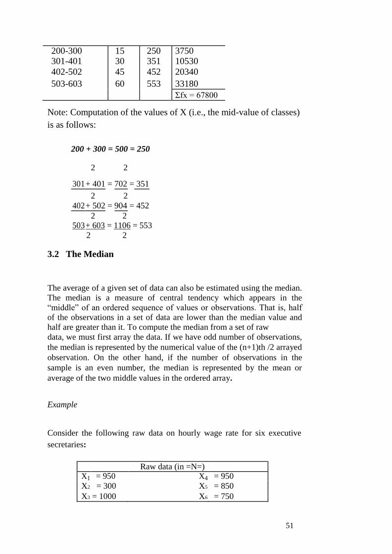
200-300 15 250 3750 301-401 30 351 10530

402-502 45 452 20340

503-603 60 553 33180

Σfx = 67800

Note: Computation of the values of X (i.e., the mid-value of classes)

is as follows:

200 + 300 = 500 = 250

2 2

301 + 401 = 702 = 351

2 2

402 + 502 = 904 = 452

2 2

503 + 603 = 1106 = 553

2 2

3.2 The Median

The average of a given set of data can also be estimated using the median.

The median is a measure of central tendency which appears in the

“middle” of an ordered sequence of values or observations. That is, half

of the observations in a set of data are lower than the median value and

half are greater than it. To compute the median from a set of raw

data, we must first array the data. If we have odd number of observations,

the median is represented by the numerical value of the (n+1)th /2 arrayed

observation. On the other hand, if the number of observations in the

sample is an even number, the median is represented by the mean or

average of the two middle values in the ordered array.

Example

Consider the following raw data on hourly wage rate for six executive

secretaries:

Raw data (in =N=)

X1 = 950 X4 = 950

X2 = 300 X5 = 850

X3 = 1000 X6 = 750

51

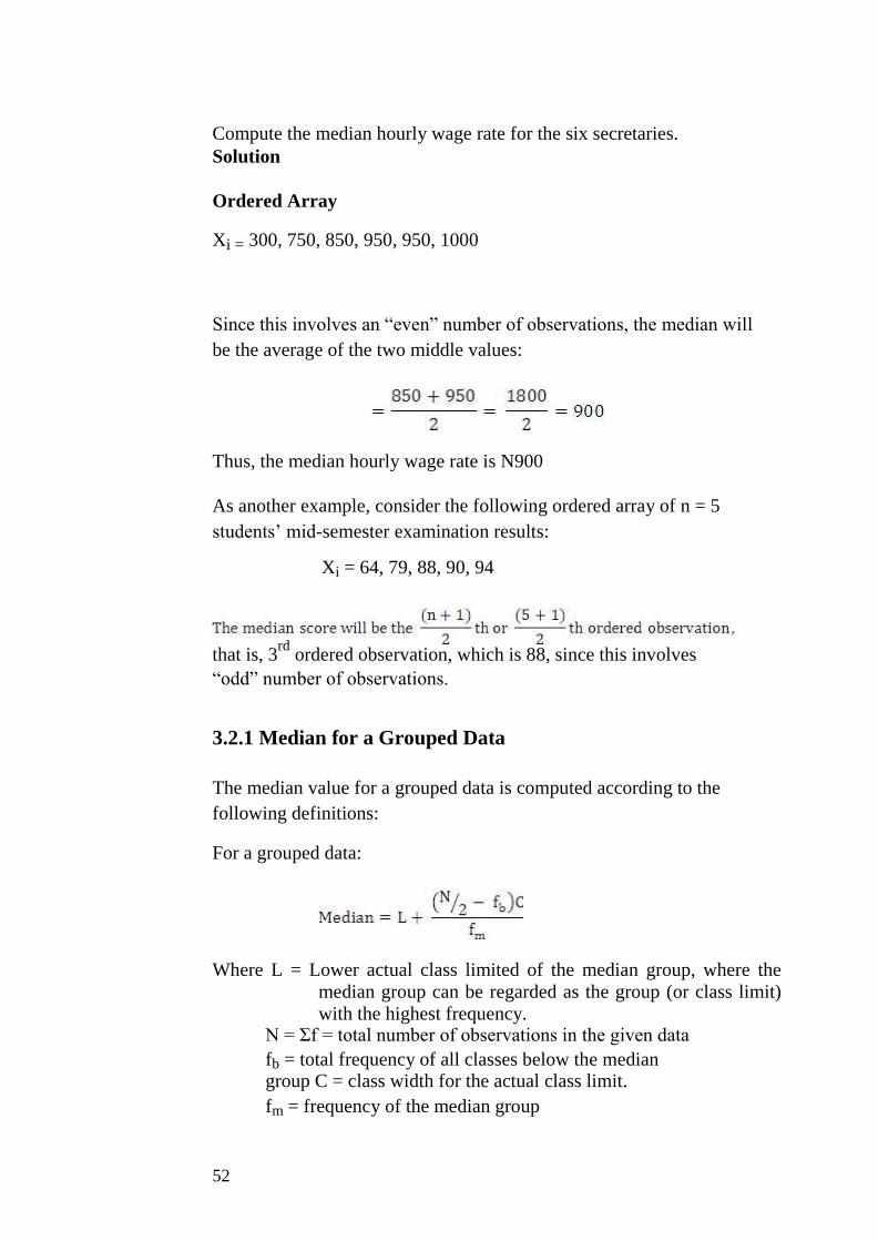
Compute the median hourly wage rate for the six secretaries.

Solution

Ordered Array

Xi = 300, 750, 850, 950, 950, 1000

Since this involves an “even” number of observations, the median will

be the average of the two middle values:

Thus, the median hourly wage rate is N900

As another example, consider the following ordered array of n = 5

students’ mid-semester examination results:

Xi = 64, 79, 88, 90, 94

that is, 3rd

ordered observation, which is 88, since this involves

“odd” number of observations.

3.2.1 Median for a Grouped Data

The median value for a grouped data is computed according to the

following definitions:

For a grouped data:

Where L = Lower actual class limited of the median group, where the

median group can be regarded as the group (or class limit)

with the highest frequency. N = Σf = total number of observations in the given data

fb = total frequency of all classes below the median group C = class width for the actual class limit.

fm = frequency of the median group

52

Note: Class Width = Upper Class Limit – Lower Class Limit

53

Example

Giving the following table on the share prices of a quoted company

over a period of 60 days:

Price in =N= No. of Days (f) 110-114 2 115-119 6

120-124 8

125-129 12

130-134 14

135-139 8

140-144 6

145-149 4

Σf = 60

Find the median share price.

Solution

We re-tabulate the data to get the needed computational values:

State Class Limits Actual Class Limits Frequency (f) 100-114 109.5-114.5 2 115-119 114.5-119.5 6

120-124 119.5-124.5 8

125-129 124.5-129.5 12

130-134 129.5-134.5 14

130-139 134.5-139.5 8

140-144 139.5-144.5 6

145-149 144.5-149.5 4

f=60

From the re-tabulated data, the median group, that is, the group with the

highest frequency (14) is (129.5-134.5).

By definition,

Where L = 129.5; N = 60; fb = 12+8+6+2 = 28; C = 5; fm = 14.

54

= 129.5 + 0.71 = 130.21

Thus, the median share price is N130.21 3.3 The Mode

The mode is a quick measure of central tendency or average. The mode is

the most typical or most frequently observed value in a given set of data.

It is the observation with the highest frequency in a given set.

For the set of data, X = 1,2,2,4, the value with the highest frequency is

2. Hence, the mode for the given data is 2.

3.4.1 Mode for a Grouped Data

The computational process for the mode of a grouped data is similar to

that of the median. The process is as follows:

Where L = Lower actual class limit of the model group

fm = frequency of the model group

fL = frequency of the group before the model group

fh = frequency of the group after the model group

C = class width for the actual class limit

Example

Consider the following data on the sales by 90 sales representatives:

Sales (N’000s) No. of Sales Reps.(f) 10 – 15 10 16 – 21 36

22 – 27 28

28 – 33 10

34 – 39 6

Calculate the modal value of sales.

Solution

Re-tabulating the data, we get:

55

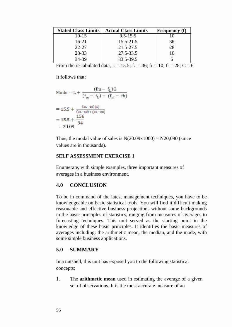
Stated Class Limits Actual Class Limits Frequency (f) 10-15 9.5-15.5 10 16-21 15.5-21.5 36

22-27 21.5-27.5 28

28-33 27.5-33.5 10

34-39 33.5-39.5 6

From the re-tabulated data, L = 15.5; fm = 36; fL = 10; fh = 28; C = 6.

It follows that:

= 20.09

Thus, the modal value of sales is N(20.09x1000) = N20,090 (since

values are in thousands).


Enumerate, with simple examples, three important measures of

averages in a business environment.

4.0 CONCLUSION

To be in command of the latest management techniques, you have to be

knowledgeable on basic statistical tools. You will find it difficult making

reasonable and effective business projections without some backgrounds

in the basic principles of statistics, ranging from measures of averages to

forecasting techniques. This unit served as the starting point in the

knowledge of these basic principles. It identifies the basic measures of

averages including: the arithmetic mean, the median, and the mode, with

some simple business applications.

5.0 SUMMARY

In a nutshell, this unit has exposed you to the following statistical

concepts:

1. The arithmetic mean used in estimating the average of a given

set of observations. It is the most accurate measure of an

56

average, and of major concern in the present discussion are three

levels of estimates:

Arithmetic Mean of observations of equal weights or

levels of importance.

Arithmetic Mean of weighted set of observations

(weighted Arithmetic Mean)

Arithmetic Mean for a grouped data (or set of

observations)

2. The median, a measure of central tendency which appears in the

“middle” of an ordered sequence of values or observations. That is,

half of the observations in a set of data are lower than the median

value and half are greater than it. 3. The mode which is a quick measure of central tendency or

average. The mode is the most typical or most frequently observed

value in a given set of data. It is the observation with the highest

frequency in a given set.


The award of a contract is based on a contractor’s scores on credibility

test over five years in business. The scores are weighted as follows:

Year: 1 2 3 4 5

Weight 1 3 5 7 9

If the score of five of the contractors (Adamu, Okoli, Babalola, Udoh

and Okoh) are as shown below:

Contractor Year

1 2 3 4 5

Adamu 62 62 50 61 48

Okoli 46 56 67 50 62

Babalola 51 54 60 55 58

Udoh 63 60 49 52 61

Okoh 58 62 60 52 70

and a contract will be awarded to the contractor with the highest

average score, which contractor will the contract, be given to?


57



edition.


UNIT 2 STATISTICAL TOOLS II: MEASURES OF

VARIABILITY OR DISPERSION

CONTENTS

1.0 Introduction

2.0 Objectives

3.0 Main Content

3.1 The Measures of Variations or Dispersion

3.1.1 The Range

3.2 The Mean Deviation (MD)

3.3 The Variance

3.4 The Standard Deviation

3.4.1 Variance and Standard Deviation for a Grouped

Data

3.5 The Coefficient of Variation

3.6 The Measures of Skewness

3.6.1 The Pearson’s No. 1 Coefficient of Skewness


4.0 Conclusion

5.0 Summary



1.0 INTRODUCTION

The second most important characteristic which describes a set of data is

the amount of variation, deviation, scatter, or spread in the data. Deviation

from an established average is a signal that a problem requiring

managerial solution exists. A sales person in a commercial bank who

consistently performs below an established average or target, for example,

signals a problem in his or her marketing activities, which requires

managerial decision. In this unit, we outline five important measures of

variations, including:

1. the range

2. mean deviation

58

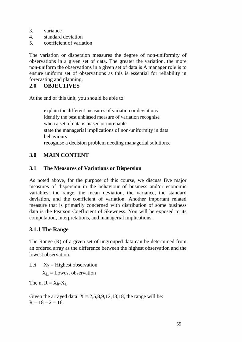
3. variance 4. standard deviation

5. coefficient of variation

The variation or dispersion measures the degree of non-uniformity of

observations in a given set of data. The greater the variation, the more

non-uniform the observations in a given set of data is A manager role is to

ensure uniform set of observations as this is essential for reliability in

forecasting and planning.

2.0 OBJECTIVES


explain the different measures of variation or deviations

identify the best unbiased measure of variation recognise

when a set of data is biased or unreliable

state the managerial implications of non-uniformity in data

behaviours

recognise a decision problem needing managerial solutions.

3.0 MAIN CONTENT

3.1 The Measures of Variations or Dispersion

As noted above, for the purpose of this course, we discuss five major

measures of dispersion in the behaviour of business and/or economic

variables: the range, the mean deviation, the variance, the standard

deviation, and the coefficient of variation. Another important related

measure that is primarily concerned with distribution of some business

data is the Pearson Coefficient of Skewness. You will be exposed to its

computation, interpretations, and managerial implications.

3.1.1 The Range

The Range (R) of a given set of ungrouped data can be determined from

an ordered array as the difference between the highest observation and the

lowest observation.

Let Xh = Highest observation

XL = Lowest observation

The n, R = Xh-XL

Given the arrayed data: X = 2,5,8,9,12,13,18, the range will be:

R = 18 – 2 = 16.

59

3.2 The Mean Deviation (MD)

The Mean Deviation can be defined simply by the following

relationship:

arithmetic mean

n = number of observation

As an example, consider again the arrayed data, X = 2,5,8,9,12,13,18.

The mean deviation, MD, can be computed as follows:

By tabulation,

X

2 -7.57 7.57 5 -2.57 2.57

8 -1.57 1.57

9 -0.57 0.57

12 2.43 2.43

13 3.43 3.43

18 8.43 8.43

Σ /X-X/= 26.57

Thus,

3.4 The Variance

The Variance for a given set of an ungrouped data can be defined by:

60

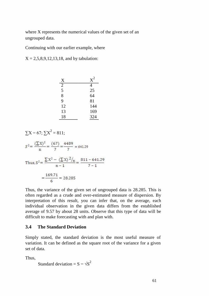
where X represents the numerical values of the given set of an

ungrouped data.

Continuing with our earlier example, where

X = 2,5,8,9,12,13,18, and by tabulation:

X X2

2 4 5 25

8 64

9 81

12 144

13 169

18 324

∑X = 67; ∑X2 = 811;

Thus, the variance of the given set of ungrouped data is 28.285. This is

often regarded as a crude and over-estimated measure of dispersion. By

interpretation of this result, you can infer that, on the average, each

individual observation in the given data differs from the established

average of 9.57 by about 28 units. Observe that this type of data will be

difficult to make forecasting with and plan with.

3.4 The Standard Deviation

Simply stated, the standard deviation is the most useful measure of

variation. It can be defined as the square root of the variance for a given

set of data.

Thus,

Standard deviation = S = √S2

61

Or,

The standard deviation for the last example is:

Again, by interpretation, this implies that each individual observation in

the given set of data deviates from the established average of 9.57 by

about 5 units.

3.4.1 Variance and Standard Deviation f or a Grouped Data

The computation of variance and standard deviation for a grouped data

is illustrated by the following example.

The Variance and Standard Deviation for a grouped data are defined by

the following formulations:

Example

The following data presents the profit ranges of 100 firms in a given

industry.

Profits (N’millions) No. of Firms (f) 10 – 15 8 16 – 21 18

22 – 27 20

28 – 33 12

34 – 39 15

40 – 45 17

46 – 51 10

∑f = n = 100

We are required to compute the variance and standard deviation of

profits within the industry.

62

Solutions

By definition,

The computational process is as follows:

Profits Frequenc y Mid-Value 2 2

(N millions) (f) (x) 10-15 8 12.5 100 156.25 1250

16-21 18 18.5 333 342.25 6160.5

22-27 20 24.5 490 600.25 12005

28-33 12 30.5 366 930.25 11163

34-39 15 36.5 547.5 1332.25 19983.75

40-45 17 42.5 722.5 1806.25 30706.25

46-51 10 48.5 485 2352.25 23522.50

∑f=n=100 ∑fx=3044 104791= ∑ fx 2

Summary

∑fx=3044

∑fx2 = 104791

It follows that:

63

Thus, the required variance and standard deviation are 122.54 and 11.07

respectively.

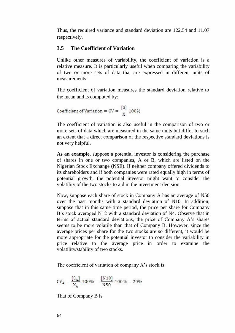
3.5 The Coefficient of Variation

Unlike other measures of variability, the coefficient of variation is a

relative measure. It is particularly useful when comparing the variability

of two or more sets of data that are expressed in different units of

measurements.

The coefficient of variation measures the standard deviation relative to

the mean and is computed by:

The coefficient of variation is also useful in the comparison of two or

more sets of data which are measured in the same units but differ to such

an extent that a direct comparison of the respective standard deviations is

not very helpful.

As an example, suppose a potential investor is considering the purchase

of shares in one or two companies, A or B, which are listed on the

Nigerian Stock Exchange (NSE). If neither company offered dividends to

its shareholders and if both companies were rated equally high in terms of

potential growth, the potential investor might want to consider the

volatility of the two stocks to aid in the investment decision.

Now, suppose each share of stock in Company A has an average of N50

over the past months with a standard deviation of N10. In addition,

suppose that in this same time period, the price per share for Company

B’s stock averaged N12 with a standard deviation of N4. Observe that in

terms of actual standard deviations, the price of Company A’s shares

seems to be more volatile than that of Company B. However, since the

average prices per share for the two stocks are so different, it would be

more appropriate for the potential investor to consider the variability in

price relative to the average price in order to examine the

volatility/stability of two stocks.

The coefficient of variation of company A’s stock is

That of Company B is

64

It follows that relative to the average, the share price of company B’s

stock is much more variable/unstable than that of Company A.

3.6 The Measures of Skewness

The measures of skewness are generally called Pearson’s first

coefficient of skewness and Pearson’s second coefficient of skewness.

Measures of skewness are used in determining the degree of asymmetry

of a distribution; a distribution which is not symmetrical is said to be

skewed.


The formula used in calculating Pearson’s No. 1 coefficient is:

Notice that the mean, the mode, and the standard deviation are all

expressed in the units of the original data. When the difference between

the mean and the mode is computed as a fraction of the standard

deviation (or average spread of the data around the mean), the original

units cancel out in the fraction. The result will be a coefficient of

skewness, a number which tells you the extent of the skewness in the

distribution.

Example

Consider a set of data on monthly sales of a company’s product, the

mean of which was found to be N240, 000; the mode found to be N135,

000; and the standard deviation found to be N85, 000. The Pearson’s

No. 1 Coefficient of skewness would be calculated as follows:

= 1.24

Generally, a complete absence of skewness would have a coefficient of

skewness equal to zero. In our example, since the mean was larger

65

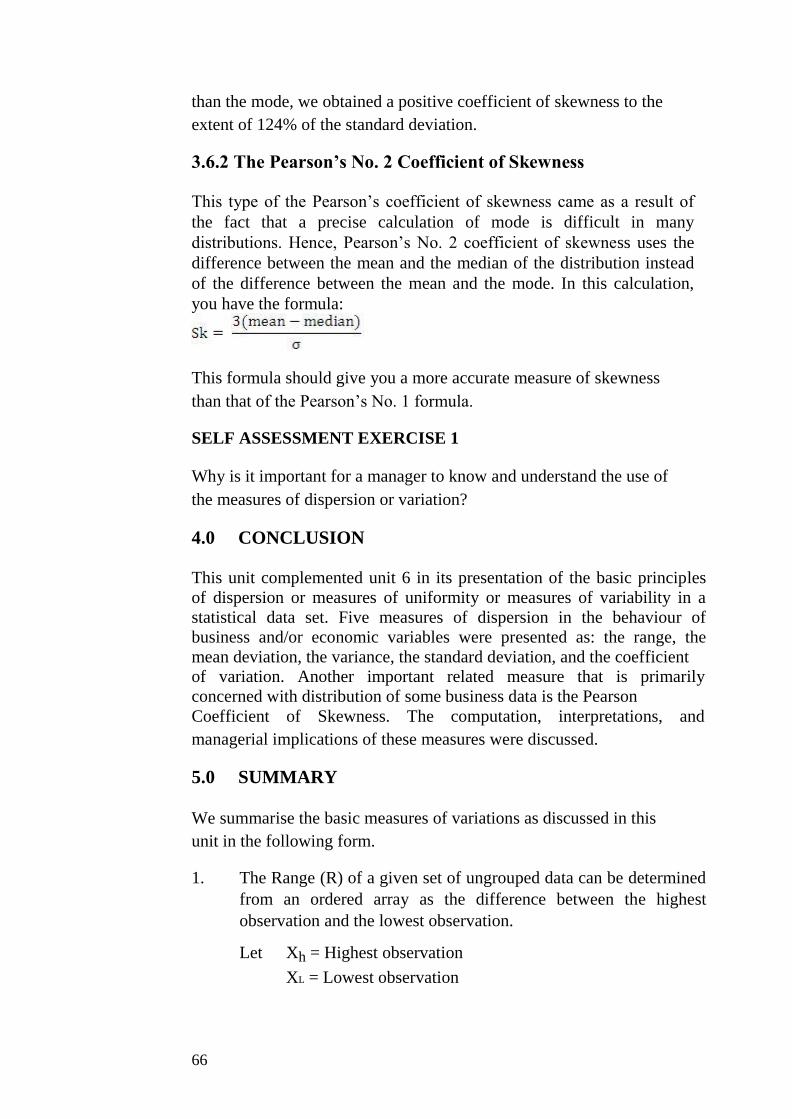
than the mode, we obtained a positive coefficient of skewness to the

extent of 124% of the standard deviation.


This type of the Pearson’s coefficient of skewness came as a result of

the fact that a precise calculation of mode is difficult in many

distributions. Hence, Pearson’s No. 2 coefficient of skewness uses the

difference between the mean and the median of the distribution instead

of the difference between the mean and the mode. In this calculation,

you have the formula:

This formula should give you a more accurate measure of skewness

than that of the Pearson’s No. 1 formula.


Why is it important for a manager to know and understand the use of

the measures of dispersion or variation?

4.0 CONCLUSION

This unit complemented unit 6 in its presentation of the basic principles

of dispersion or measures of uniformity or measures of variability in a

statistical data set. Five measures of dispersion in the behaviour of

business and/or economic variables were presented as: the range, the

mean deviation, the variance, the standard deviation, and the coefficient

of variation. Another important related measure that is primarily

concerned with distribution of some business data is the Pearson

Coefficient of Skewness. The computation, interpretations, and

managerial implications of these measures were discussed.

5.0 SUMMARY

We summarise the basic measures of variations as discussed in this

unit in the following form.

1. The Range (R) of a given set of ungrouped data can be determined

from an ordered array as the difference between the highest

observation and the lowest observation.

Let Xh = Highest observation

XL = Lowest observation

66

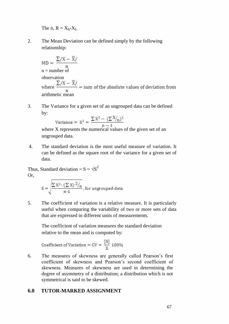
The n, R = Xh-XL

2. The Mean Deviation can be defined simply by the following

relationship:

n = number of

observation

arithmetic mean

3. The Variance for a given set of an ungrouped data can be defined

by:

where X represents the numerical values of the given set of an

ungrouped data. 4. The standard deviation is the most useful measure of variation. It

can be defined as the square root of the variance for a given set of

data.

Thus, Standard deviation = S = √S2

Or,

5. The coefficient of variation is a relative measure. It is particularly

useful when comparing the variability of two or more sets of data

that are expressed in different units of measurements.

The coefficient of variation measures the standard deviation

relative to the mean and is computed by: 6. The measures of skewness are generally called Pearson’s first

coefficient of skewness and Pearson’s second coefficient of

skewness. Measures of skewness are used in determining the

degree of asymmetry of a distribution; a distribution which is not

symmetrical is said to be skewed.


67

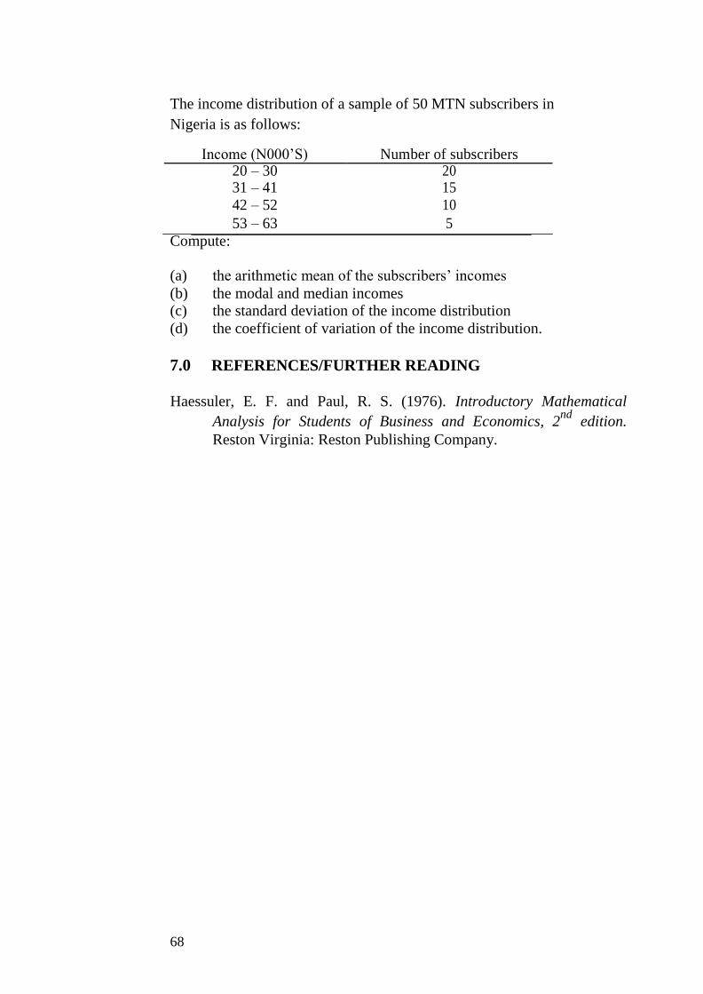
The income distribution of a sample of 50 MTN subscribers in

Nigeria is as follows:

Income (N000’S) Number of subscribers 20 – 30 20 31 – 41 15

42 – 52 10

53 – 63 5

Compute:

(a) the arithmetic mean of the subscribers’ incomes (b) the modal and median incomes (c) the standard deviation of the income distribution

(d) the coefficient of variation of the income distribution.




edition.


68

UNIT 3 STATISTICAL TOOLS III: SETS AND SET

OPERATIONS

CONTENTS

1.0 Introduction

2.0 Objectives

3.0 Main Content

3.1 The Theory of Sets

3.1.1 Subsets, Number of a Set, Set Equality, Universal

Set, Complement of a Set, and the Venn Diagram

3.2 Operations on Sets

3.2.1 General Solutions to Enumeration Problems

3.3 Summary of the General Enumeration Problem

4.0 Conclusion

5.0 Summary



1.0 INTRODUCTION

In this unit, we develop the basic principles of probabilistic analysis,

with special emphasis on the applications of set operations and events.

2.0 OBJECTIVES


interprete the concept of sets as they are used in mathematical

operations

explain the theory of sets and how it is used in probability

analysis.

explain set enumerations and how they can be applied in solving

business-related problems

3.0 MAIN CONTENT

3.1 The Theory of Sets

69

The theory of sets serves as a preliminary concept necessary for the

understanding of the theory of probabilities. A mathematical set is a

collection of distinct objects, often referred to as elements or members.

70

Examples

(a) The employees of a company working in the Public Relations

Department could be represented as:

PR = {Joseph, Adamu, Adebola, Nkom, Margerate}

(b) The location of shops for a big automobile parts dealer could be

represented as:

S = {Abuja, Enugu, Lagos, Aba, Onitsha, Kano, Ikot Ekpene}

3.1.1 Subsets, Number of a Set, Set Equality, Universal Set,

Complement of a Set, and the Venn Diagram

Subsets

A subset of a set, say A, is a set which contains some of the elements of

set A. For instance:

If set A = {a, e, i, o, u}, then:

X = {a, e, i} is a subset of A

Y = {e, i} is a subset of A

Z = {i, o, u} is a subset of A

The Number of a Set

The number of a set A, written as n[A], is defined as the number of

elements in set A. For example:

If A = {a, e, i, o, u}, then n[A] = 5 (that is, 5 elements in set A).

Set Equality

Two sets are said to be equal only when they have identical elements.

For example:

If A = {1, 2, 3} and B = {1, 2, 3}, then Set A = Set B.

Universal Set

A universal set, denoted by U is a set containing different subsets of its

elements. For example, a combination of different behaviours in a given

population can be considered as universal, while a selected sample of

such behaviours are referred to as the subsets. A set of all English

71

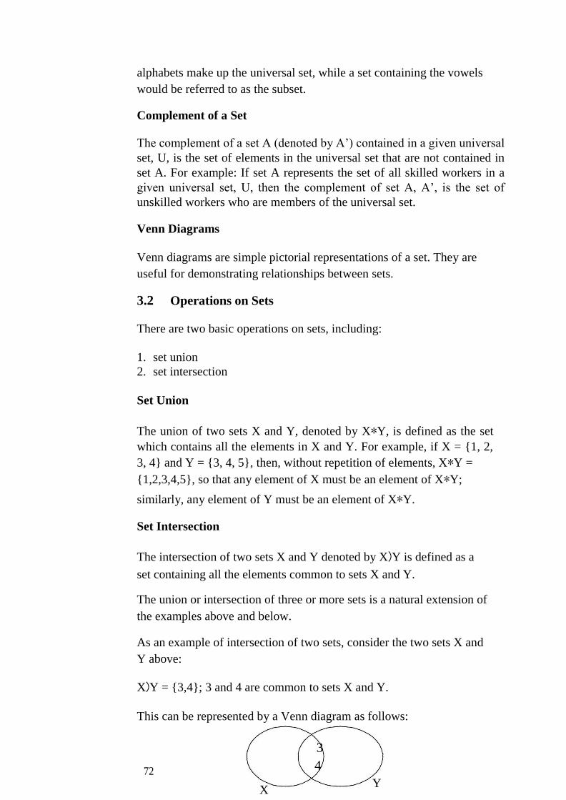
alphabets make up the universal set, while a set containing the vowels

would be referred to as the subset.

Complement of a Set

The complement of a set A (denoted by A’) contained in a given universal

set, U, is the set of elements in the universal set that are not contained in

set A. For example: If set A represents the set of all skilled workers in a

given universal set, U, then the complement of set A, A’, is the set of

unskilled workers who are members of the universal set.

Venn Diagrams

Venn diagrams are simple pictorial representations of a set. They are

useful for demonstrating relationships between sets.

3.2 Operations on Sets

There are two basic operations on sets, including:

1. set union 2. set intersection

Set Union

The union of two sets X and Y, denoted by X∗Y, is defined as the set

which contains all the elements in X and Y. For example, if X = {1, 2,

3, 4} and Y = {3, 4, 5}, then, without repetition of elements, X∗Y =

{1,2,3,4,5}, so that any element of X must be an element of X∗Y;

similarly, any element of Y must be an element of X∗Y.

Set Intersection

The intersection of two sets X and Y denoted by X)Y is defined as a

set containing all the elements common to sets X and Y.

The union or intersection of three or more sets is a natural extension of

the examples above and below.

As an example of intersection of two sets, consider the two sets X and

Y above:

X)Y = {3,4}; 3 and 4 are common to sets X and Y.

This can be represented by a Venn diagram as follows:

3

72 4

Y X

The elements {3, 4} are contained in the circle common to sets X and

Y. Set Enumeration

Set enumeration considers sets in terms of number of elements contained

within the various areas defined by their union or intersection. Identifying

the number of elements in these areas is known as set enumeration. As an

illustration, consider the following enumeration problem.

Suppose an accounting firm currently employs 16 staff members. Given

that three staff members have no formal qualifications, and of the seven

staff members, who are graduates, 5 are also qualified as chartered

accountants, it is possible to evaluate: (a) the number of staff who are

non-graduates, chartered accountants and (b) the number of graduates

who are not qualified chartered accountants.

The two values can be calculated as follows:

1. Since three staff members have no formal qualifications, there

should be 16– 3 = 13 staff members with at least one of the two

qualifications that is, a graduate or a chartered accountant. 2. But there are 7 staff members who are graduates, which implies

that 16 –7–3= 6 must be non-graduate, qualified chartered

accountants, which gives the answer to possibility (a) above. 3. In addition, since 5 staff members are qualified chartered

accountants and graduates, there would be 7 – 5 = 2 staff who are

graduates only. This gives answer to possibility (b) above.

In an extended problem, the above approach is not structured enough for

the solution. In the following discussions, we present a more structured

procedure which solves the above problems and forms a basis for more

logical approach for solving enumerations problems in general.

3.2.1 General Solutions to Enumeration Problems

The above problem can be solved stepwise as follows:

73

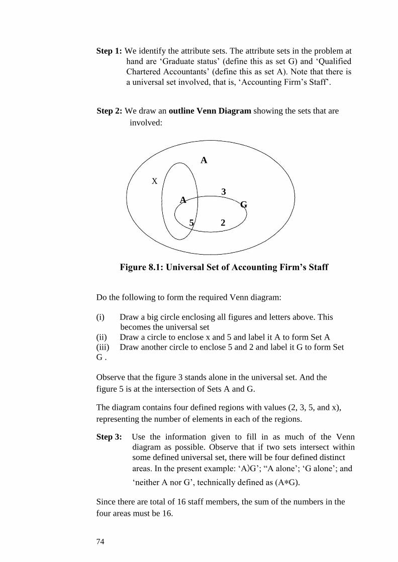
Step 1: We identify the attribute sets. The attribute sets in the problem at

hand are ‘Graduate status’ (define this as set G) and ‘Qualified

Chartered Accountants’ (define this as set A). Note that there is

a universal set involved, that is, ‘Accounting Firm’s Staff’.

Step 2: We draw an outline Venn Diagram showing the sets that are

involved:

A

X

3 A

G

5 2

Figure 8.1: Universal Set of Accounting Firm’s Staff

Do the following to form the required Venn diagram:

(i) Draw a big circle enclosing all figures and letters above. This

becomes the universal set

(ii) Draw a circle to enclose x and 5 and label it A to form Set A (iii) Draw another circle to enclose 5 and 2 and label it G to form Set G .

Observe that the figure 3 stands alone in the universal set. And the

figure 5 is at the intersection of Sets A and G.

The diagram contains four defined regions with values (2, 3, 5, and x),

representing the number of elements in each of the regions.

Step 3: Use the information given to fill in as much of the Venn

diagram as possible. Observe that if two sets intersect within

some defined universal set, there will be four defined distinct

areas. In the present example: ‘A)G’; “A alone’; ‘G alone’; and

‘neither A nor G’, technically defined as (A∗G).

Since there are total of 16 staff members, the sum of the numbers in the

four areas must be 16.

74

Interpreting the Venn diagrams above:

1. 5 staff members are graduates and qualified chartered

Accountants. This number is thus entered in the ‘(A)G)’ area. 2. Since there are 7 graduates in all, there must be 7 – 5 = 2

graduates who are not chartered accountants. This number is

thus entered in the ‘G alone’ area. 3. three (3) of the staff had no qualifications at all. This number is

thus entered in the ‘neither A nor G or A∗G’ area.

Step 4: Finally, we evaluate the number of elements in any remaining

unknown areas. As indicated by the above diagram, x is an

unknown number in the area ‘A alone’. We need to solve for x

as required, that is, the number of chartered accountants who are

not graduates.

Putting x as the unknown number:

3 + 5 + 2 + x = 16 (the total number of staff)

Solving for x, we get: x = 6.

3.3 Summary of the General Enumeration Problems

Note in particular that there are:

(a) 4 distinct areas for two attribute sets, and

(b) 8 distinct areas for three attribute sets.

The general procedure for solving enumeration problems follows the

following steps:

Step 1: Identify the attribute sets

Step 2: Draw an outline Venn diagram

Step 3: Use the information given to fill in as much of the diagram

Step 4:

as possible

Evaluate the number of elements in unknown areas.

Consider the following example:

A survey was carried out by a researcher, one of the aims being to

discover the extent to which computers are being used by firms in a given

area. 32 firms had both stock control and payroll computerised, 65 firms

had just one of these two functions computerised, and 90 firms had a

computerised payroll. If 22 firms had neither of these functions

computerised, how many firms were included in the survey?

75

Solution

Step 1: The two attributes involved are computerised payroll, with

set (say P), and computerised stock control, with set (say S).

Step 2: Using standard notations,

Let p = number of firms with a computerised payroll

only; s = number of firms with a computerised stock

control only;

ps = number of firms with both payroll and stock

control computerised; and

x = number of firms with neither functions computerised,

construct a Venn diagram describing the situation.

Step 3: The following equations can be set up from the given

information.

ps = 32 (1)

p + s = 65 (2)

ps + p = 90 (3)

x = 22 (4)

Step 4: Substituting for ps = 32 in equation 3, we get p = 58

Substituting for p = 58 in equation, we get s = 7.

It follows that the number of firms included in the survey

equals:

p + s + ps + x = 58 + 7 + 32 + 22 = 119.


1. If X = {a,4,3,d,e}; Y = {3,d,e,f}; and Z = {a,3,d,e,g,h} within a

universal set of U = {a,4,3,d,e,f,g,h.i}, list the elements of the

following sets:

(a) X∗Y (b) X)Y (c) Y’)Z’ (d) X∗Y)Z

4.0 CONCLUSION

The theory of set is currently used in several business operations. It is

used in much software programming, in the study of consumer behaviour,

and in solving complex business problems. The unit has put

76

together some preliminary concepts in set notations. You must have

been exposed to the simple operations on sets.

5.0 SUMMARY

The basic points in our discussions on sets and set operations can be

summarised in few words as follows.

A mathematical set is a collection of distinct objects, often referred to

as elements or members.

The number of a set A, written as n[A], is defined as the number of

elements in set A.

There are two basic operations on sets, including:

1. set union 2. set intersection

Set enumeration considers sets in terms of number of elements contained

within the various areas defined by their union or intersection. Identifying

the number of elements in these areas is known as set enumeration.

The general procedure for solving enumeration problems follows the

following steps:

Step 1: Identify the attribute sets

Step 2: Draw an outline Venn diagram

Step 3: Use the information given to fill in as much of the diagram as

Step 4:

Possible

Evaluate the number of elements in unknown areas.


A and B are two intersecting sets and a, b, ab, and # represent the usual

symbols for the number of elements contained in the four defined areas of

the associated Venn diagram. Find the values of ab and a if:

n[A] = 28; a +b = 36; and, # = 48. The number of elements in the

universal set is 96


A. Francis (1998). Business Mathematics and Statistics, 5th

edition.

Great Britain: Ashford Colour Press.

77

UNIT 4 STATISTICAL TOOLS IV: PROBABILITY

THEORY AND APPLICATIONS

CONTENTS

1.0 Introduction

2.0 Objectives

3.0 Main Content

3.1 Definitions of Probability

3.2 Law of Probability

3.3 Computational Formula for Multiple Occurrence of an

Event

3.4 Joint, Marginal, Conditional Probabilities, and the Bayes

Theorem

3.4.1 Joint Probabilities

3.4.2 Marginal Probabilities

3.4.3 Conditional Probability

3.4.4 The Bayes Theorem

3.5 Probability and Expected Values

4.0 Conclusion

5.0 Summary



1.0 INTRODUCTION

In this unit, we pay a special attention to the concept of probability,

probability laws, computation of probabilities, and their applications to

business decisions. At the end of this lecture, students will be expected to

be able to make effective decisions under uncertainties.

The basic elements of probability theory are the outcomes of the process

or phenomenon under study. Each possible type of occurrence is referred

to as an event. The collection of all the possible events is called the

sample space.

A compound or joint event is an event that has two or more

characteristics. For example, the event of a student who is “an economics

major and B or above average” is a joint or compound event since the

student must be an economics major and have a B or above average.

The event “black ace” is also a compound event since the card must be

both black and ace in order to qualify as a black ace.

78

Probability is a concept that most people understand naturally, since such

words as “chance,” “likelihood,” “possibility” and “proportion are used as

part of everyday speech. For example, most of the following, which might

be heard in any business situation, are in fact statements of probability.

a) “There is a 30% chance that this job will not be finished in time”. b) “There is every likelihood that the business will make a profit

next year”. c) “Nine times out of ten, he arrives late for his appointments”.

In statistical sense, probability simply puts a well defined structure

around the concept of everyday probability, enabling a logical approach

to problem solving to be followed.

2.0 OBJECTIVES


explain the theory of probability

define probability

recognise the laws of probability

calculate

probabilities

apply probabilities in making decisions involving uncertainties.

3.0 MAIN CONTENT

3.1 Definitions of Probability

There are basically two separate ways of calculating probability.

1. Calculation based on theoretical probability. This is the name

given to probability that is calculated without an experiment that

is, using only information that is known about the physical

situation. 2. Calculation based on empirical probability. This is probability

calculated using the results of an experiment that has been

performed a number of times. Empirical probability is often

referred to as relative frequency or Subjective probability.

79

Definition of Theoretical Probability

Let E represent an event of an experiment that has an equally likely

outcome set, U, then the theoretical probability of event E occurring

when the experiment is written as Pr (E) and given by:

Where n (E) = the number of outcomes in event set E

n (U) = total possible number of outcomes in outcome set, U.

If, for example, an ordinary six-sided die is to be rolled, the equally likely

outcome set, U, is {1,2,3,4,5,6} and the event “even number” has event

set {2,4,6}. It follows that the theoretical probability of obtaining an even

number can be calculated as:

Other Examples

A wholesaler stocks heavy (2B), medium (HB), fine (2H) and extra fine

(3H) pencils which come in packs of 10. Currently in stock are 2 packs

of 3H, 14 packs of 2H, 35 packs of HB and 8 packs of 2B. If a pack of

pencil is chosen at random for inspection, what is the probability that

they are:

(a) medium (b) heavy (c ) not very fine

(d) neither heavy nor medium?

Solutions

80

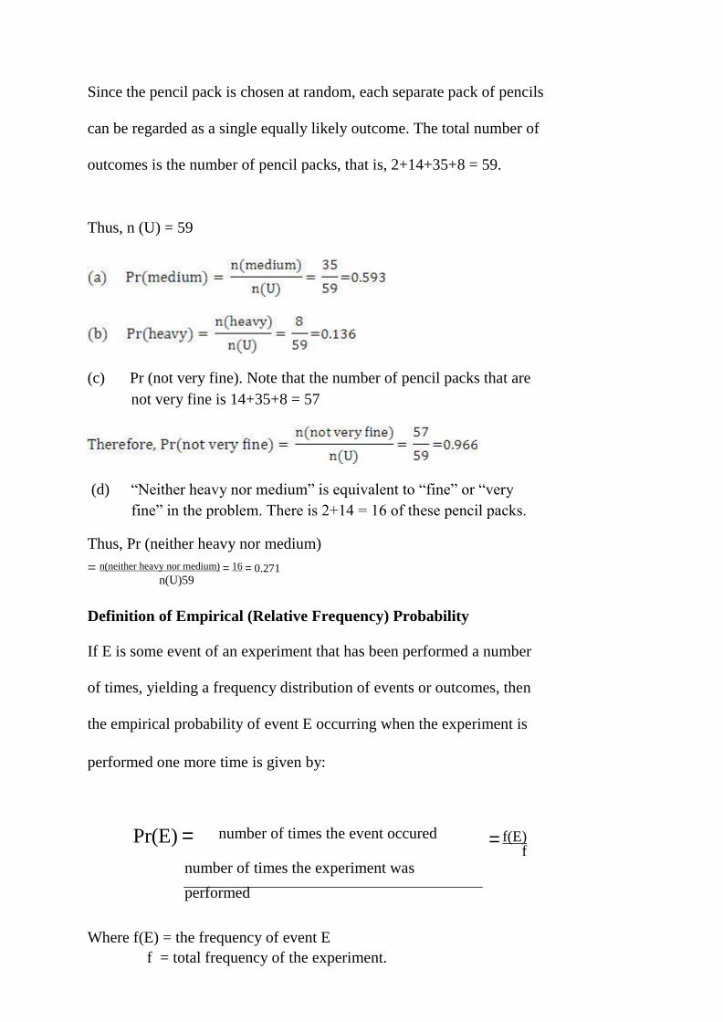
Since the pencil pack is chosen at random, each separate pack of pencils

can be regarded as a single equally likely outcome. The total number of

outcomes is the number of pencil packs, that is, 2+14+35+8 = 59.

Thus, n (U) = 59

(c) Pr (not very fine). Note that the number of pencil packs that are

not very fine is 14+35+8 = 57

(d) “Neither heavy nor medium” is equivalent to “fine” or “very

fine” in the problem. There is 2+14 = 16 of these pencil packs.

Thus, Pr (neither heavy nor medium)

= n(neither heavy nor medium) = 16 = 0.271 n(U)59

Definition of Empirical (Relative Frequency) Probability

If E is some event of an experiment that has been performed a number

of times, yielding a frequency distribution of events or outcomes, then

the empirical probability of event E occurring when the experiment is

performed one more time is given by:

Pr(E) = number of times the event occured

number of times the experiment was

performed

Where f(E) = the frequency of event E

f = total frequency of the experiment.

= f(E) f

Put differently, the empirical probability of an event E occurring is simply

the proportion of times that event E actually occurred when the

experiment was performed.

For example, if, out of 60 orders received so far this financial year, 12

were not completely satisfied, the proportion, 12/60 = 0.2 is the empirical

probability that the next order received will not be completely satisfied.

Other Examples

A number of families of a particular type were measured by the number

of children they have, given the following frequency distribution:

Number of children: 0 1 2 3 4 5 or more

Number of families: 12 28 22 8 2 2

Use this information to calculate the (relative frequency) probability

that another family of this type chosen at random will have:

(a) 2 children (b) 3 or more children

(c) less than 2 children

Solutions

Here, f = total number of families = 74

(a) Pr (2 children) = f(2 children) = 22 = 0.297

74 74

(b) f (3 or more children) = 8+2+2 = 12 Thus,

Pr(3 or more children = 12 = 0.162

74

(c) Pr(less than 2 children) = f (less than 2 children) = 12 + 28 = 0.541 f 74

3.2 Laws of Probability

There are four basic laws of probability.

82

1. Addition Law for mutually exclusive events 2. Addition Law for events that are not mutually exclusive 3. Multiplication Law for Independent events 4. Multiplication Law for Dependent events.

Addition Law for Mutually Exclusive Events

Two events are said to be mutually exclusive events if they cannot occur

at the same time. The addition law states that if events A and B are

mutually exclusive events, then: Pr (A or B) = Pr (A) + Pr (B)

Examples

The purchasing department of a big company has analysed the number

of orders placed by each of the 5 departments in the company by type as

follows:

83

Table 9.1: Depart mental Orders

Type of Department

order

Sales Purchasing Production Accounts Maintenance Total Consumables 10 12 4 8 4 38

Equipment

1 3 9 1 1 15

Special

0 0 4 1 2 7

Total 11 15 17 10 7 60

An error has been found in one of these orders. What is the probability

that the incorrect order:

a) came from maintenance? b) came from production?

c) came from maintenance or production? d) came from neither maintenance nor production?

Solutions

a) Since there are 7 maintenance orders out of the 60,

Pr(maintenance) = 7 = 0.117

60

b) Similarly, Pr (Production) = 17 = 0.283

60

c) Maintenance and production departments are two mutually

exclusive events so that, Pr(maintenance or production) = Pr(maintenance) + Pr(production = 0.117 + 0.283 = 0.40

d) Pr (neither maintenance nor production) = 1-Pr (maintenance or production) = 1-0.4 = 0.6

Addition Law for Events that are Not Mutually Exclusive Events

If events A and B are not mutually exclusive, that is, they can either

occur together or occur separately, then according to the Law:

Pr (A or B or Both) = Pr(A)+Pr(B) – Pr(A).Pr(B)

Example

Consider the following contingency table for the salary range of 94

employees:

84

Table 9.2: Contingency Table for the Salary range of 94

Employees

Salary/month Men Women Total

N 10,000 and above 20 37 57

Below 10,000 15 22 37

Total 35 59 94

What is the probability of selecting an employee who is a man or earns

below N10, 000 per month?

Solution

The two events of being a man and earning below N10, 000 is not

mutually exclusive.

It follows that:

= 35 + 37 (35)(37)

94 94 (94)(94)

= 0.372+0.394 - (0.372)(0.394) = 0.766 - 0.147

= 0.619 or 61.9%

Multiplication Law for Independent Events

This law states that if A and B are independent events, then:

Pr (A and B) = Pr (A). Pr (B)

As an example, suppose, in any given week, the probability of an

assembly line failing is 0.03 and the probability of a raw material shortage

is 0.1.

If these two events are independent of each other, then the probability

of an assembly line failing and a raw material shortage is given by:

Pr (Assembly line failing and Material shortage) = (0.03)(0.1)

= 0.003

Multiplication Law for Dependent Events

This Law states that if A and B are dependent events, then:

85

Pr (A and B) = Pr(A).Pr(B/A)

Note that Pr (B/A) in interpreted as probability of B given that event A

has occurred.

Example

A display of 15 T-shirts in a Sports shop contains three different sizes:

small, medium and large. Of the 15 T-shirts:

3 are small

6 are medium

6 are large.

If two T-shirts are randomly selected from the T-shirts, what is the

probability of selecting both a small T-shirt and a large T-shirt, the first

not being replaced before the second is selected?

Solution

Since the first selected T-shirt is not replaced before the second T-shirt is selected, the two events are said to be dependent events.

It follows that:

Pr (Small T-shirt and Large T-shirt)

= Pr(Small).Pr(Large/Small)

= (3/15)(4/14)

= (0.2)(0.429) = 0.086

3.3 Computational Formula for Multiple Occurrence of an

Event

The probability of an event, E occurring X times in n number of trials

are given by the formula:

Pr (En

x ) = Cn, xpxq

(n – x)

Where Cn,x =

n!

X !(n x)!

p = probability of success

q = probability of failure

p + q = 1

86

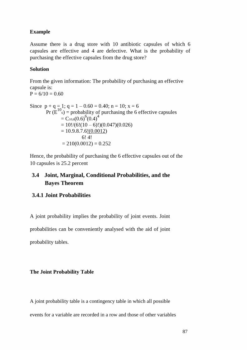
Example

Assume there is a drug store with 10 antibiotic capsules of which 6

capsules are effective and 4 are defective. What is the probability of

purchasing the effective capsules from the drug store?

Solution

From the given information: The probability of purchasing an effective

capsule is:

P = 6/10 = 0.60

Since p + q = 1; q = 1 – 0.60 = 0.40; n = 10; x = 6

Pr (E10

6) = probability of purchasing the 6 effective capsules

= C10,6(0.6)6(0.4)

4

= 10!/(6!(10 – 6)!)(0.047)(0.026)

= 10.9.8.7.6!(0.0012)

6! 4!

= 210(0.0012) = 0.252

Hence, the probability of purchasing the 6 effective capsules out of the

10 capsules is 25.2 percent

3.4 Joint, Marginal, Conditional Probabilities, and the

Bayes Theorem

3.4.1 Joint Probabilities

A joint probability implies the probability of joint events. Joint

probabilities can be conveniently analysed with the aid of joint

probability tables.

The Joint Probability Table

A joint probability table is a contingency table in which all possible

events for a variable are recorded in a row and those of other variables

87

are recorded in a column, with the values listed in corresponding cells

as in the following example.

Example

Consider a research activity with the following observations on

the number of customers that visit XYZ supermarket per day. The

observations (or events) are recorded in a joint probability table

as follows:

Table 9.3: Joint Probability Table

Age (Years) Male (M) Female (F) Total

Below 30 (B) 60 70 130

30 and Above (A) 60 20 80

Total 120 90 210

We can observe four joint events from the above table:

Below 30 and Male (B)M) = 60

Below 30 and Female (B)F) = 70

30 and Above and Male (A)M) = 60

30 and Above and Female (A)F) = 20

Total events or sample space = 210

The joint probabilities associated with the above joint events are: Pr(B) M) = 60 = 0.2857 210

88

Pr(B ) F ) = 70

= 0.3333 210

Pr( A ) M ) = 60

= 0.2857 210

Pr( A ) F ) = 20

= 0.0952 210

3.4.2 Marginal Probabilities

The Marginal Probability of an event is its simple probability of

occurrence, given the sample space. In the present discussion, the results

of adding the joint probabilities in rows and columns are known as

marginal probabilities.

The marginal probability of each of the above events:

Male (M), Female (F), Below 30 (B), and

Above 30 (A) are as follows:

Pr (M) = Pr(B)M) + Pr(A)M) = 0.2857 + 0.2857 = 0.57

Pr (F) = Pr(B)F)+Pr(A)F) = 0..3333 + 0.0952 = 0.43

Pr (B) = Pr(B)M)+Pr(B)F) = 0.2857+0.3333 = 0.62

Pr (A) = {r(A)M)+Pr(A)F) = 0.2857+0.0952 = 0.38

The joint and marginal probabilities above can be summarised in a

contingency table as follows:

Table 9.4: Joint and Marginal Probability Table.

Age Male (M) Female (F) Marginal Probability

Below 30 (B) 0.2857 0.3333 0.62

30 and Above (A) 0.2857 0.0952 0.38

Marginal Probability 0.57 0.43 1.00

3.4.3 Conditional Probability

Assuming two events, A and B, the probability of event A, given that

event B has occurred is referred to as the conditional probability of event

A.

In symbolic term:

Pr( A ) = Pr (A/B) = Pr(A) and Pr(B)

Pr(B)

89

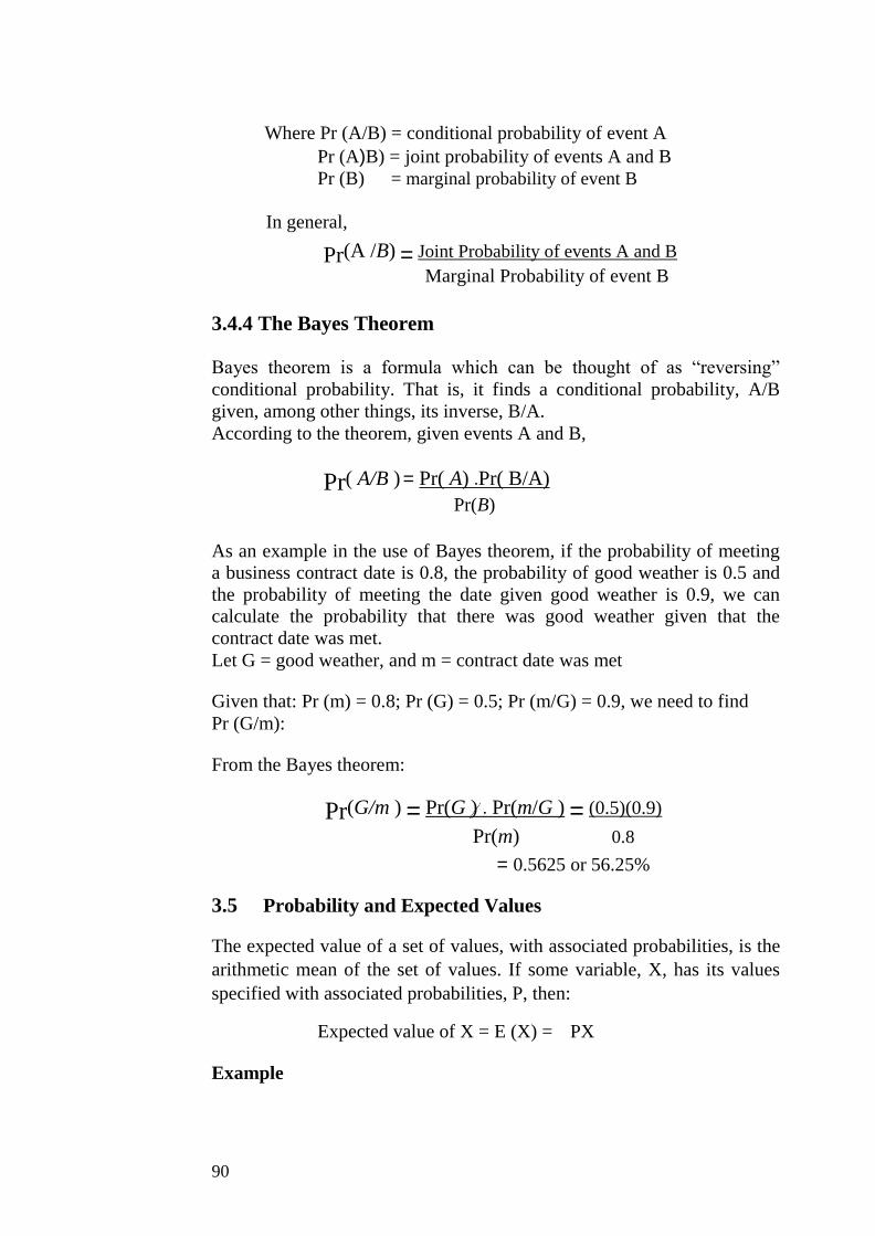
Where Pr (A/B) = conditional probability of event A

Pr (A)B) = joint probability of events A and B

Pr (B) = marginal probability of event B

In general,

Pr(A /B) = Joint Probability of events A and B

Marginal Probability of event B

3.4.4 The Bayes Theorem

Bayes theorem is a formula which can be thought of as “reversing”

conditional probability. That is, it finds a conditional probability, A/B

given, among other things, its inverse, B/A.

According to the theorem, given events A and B,

Pr( A/B ) = Pr( A) .Pr( B/A)

Pr(B)

As an example in the use of Bayes theorem, if the probability of meeting

a business contract date is 0.8, the probability of good weather is 0.5 and

the probability of meeting the date given good weather is 0.9, we can

calculate the probability that there was good weather given that the

contract date was met.

Let G = good weather, and m = contract date was met

Given that: Pr (m) = 0.8; Pr (G) = 0.5; Pr (m/G) = 0.9, we need to find

Pr (G/m):

From the Bayes theorem:

Pr(G/m ) = Pr(G ) . Pr(m/G ) = (0.5)(0.9)

Pr(m) 0.8

= 0.5625 or 56.25%

3.5 Probability and Expected Values

The expected value of a set of values, with associated probabilities, is the

arithmetic mean of the set of values. If some variable, X, has its values

specified with associated probabilities, P, then:

Expected value of X = E (X) = PX

Example

90

An ice-cream salesman divides his days into ‘Sunny’ ‘Medium’ or ‘Cold’.

He estimates that the probability of a sunny day is 0.2 and that 30% of his

days are cold. He has also calculated that his average revenue on the three

types of days is N220, N130, and N40 respectively. If his average total

cost per day is N80, calculate his expected profit per day.

Solution

We first calculate the different values of profit that are possible since we

are required to calculate expected profit per day, as well as their

respective probabilities.

Given that Pr (sunny day) = 0.2; Pr (cold day) = 0.3

Since in theory, Pr (sunny day) + Pr (cold day) +Pr (medium day) = 1

It follows that:

Pr (medium day) = 1 - 0.2 - 0.3 = 0.5

The total costs are the same for any day (N80), so that the profits that the

salesman makes on each day of the three types of day are:

Sunny day: N (220-80) = N140

Medium day: N (130-80) = N50

Cold day: N (40-80) = -N40 (loss)

We can summarise the probability table as follows:

Table 9.5: Probability Table

Profit (N) Sunny Medium Cold 140 50 -40

Probability 0.2 0.5 0.3

From this Table, the expected profit per day is:

E (profit) = N (0.2 (140) + 0.5 (50) – 0.3 (40)) =

N41 SELF ASSESSMENT EXERCISE 2

1. What do we mean by the terms “mutually exclusive events” and

“independent events?” 2. State, with simple examples, the four laws of probability.

4.0 CONCLUSION

Probability is a concept that most people understand naturally, since

such words as “chance,” “likelihood,” “possibility” and “proportion are

91

used as part of everyday speech. It is a term used in making decisions

involving uncertainty. Though the concept is often viewed as very

abstract and difficult to relate to real world activities, it remains the best

tool for solving uncertainties problems.

To remove some of the abstract nature of probabilities, this unit has

provided you with the simplest approach to understanding and

calculating, as well as applying the probability concept. It defines

probability in two basic forms:

(i) the theoretical definition; and (ii) the empirical definition.

5.0 SUMMARY

The issues discussed in this unit can be summarised in the following

way:

there are basically two separate ways of calculating probability which

are as stated below:

i. theoretical probability: this is calculated without an experiment,

that is, using only information that is known about the physical situation.

ii. calculation based on empirical probability. This is probability

calculated using the results of an experiment that has been

performed a number of times. Empirical probability is often

referred to as Relative frequency or Subjective probability.

There are four basic laws of probability:

1. addition law for mutually exclusive events

2. addition law for events that are not mutually exclusive 3. multiplication law for independent events

4. multiplication law for dependent events.

The probability of an event, E occurring an X time in n number of trials

is given by the formula:

Pr (En

x) = Cn,xpxq

(n – x)

Where Cn,x = n!

X !(n – x)!

p = probability of success

92

q = probability of failure

p + q = 1

A joint probability implies the probability of joint events. Joint

probabilities can be conveniently analysed with the aid of joint in

which all possible events for a variable are recorded in a row and those

of other variables are recorded in a column, with the values listed in

corresponding cells.

The Marginal Probability of an event is its simple probability

of occurrence, given the sample space.

Assuming two events, A and B, the probability of event A, given that

event B has occurred is referred to as the conditional probability of

event A.

The expected value of a set of values, with associated probabilities, is the

arithmetic mean of the set of values. If some variable, X, has its values

specified with associated probabilities, P, then:

Expected value of X = E (X) = PX

93


A firm has tendered for two independent contracts. It estimates that it has

probability 0.4 of obtaining contract A and probability 0.1 of obtaining

contract B. Find the probability that the firm:

(a) obtains both contracts (b) obtains neither of the contracts

(c) obtains exactly one contract



edition.


94

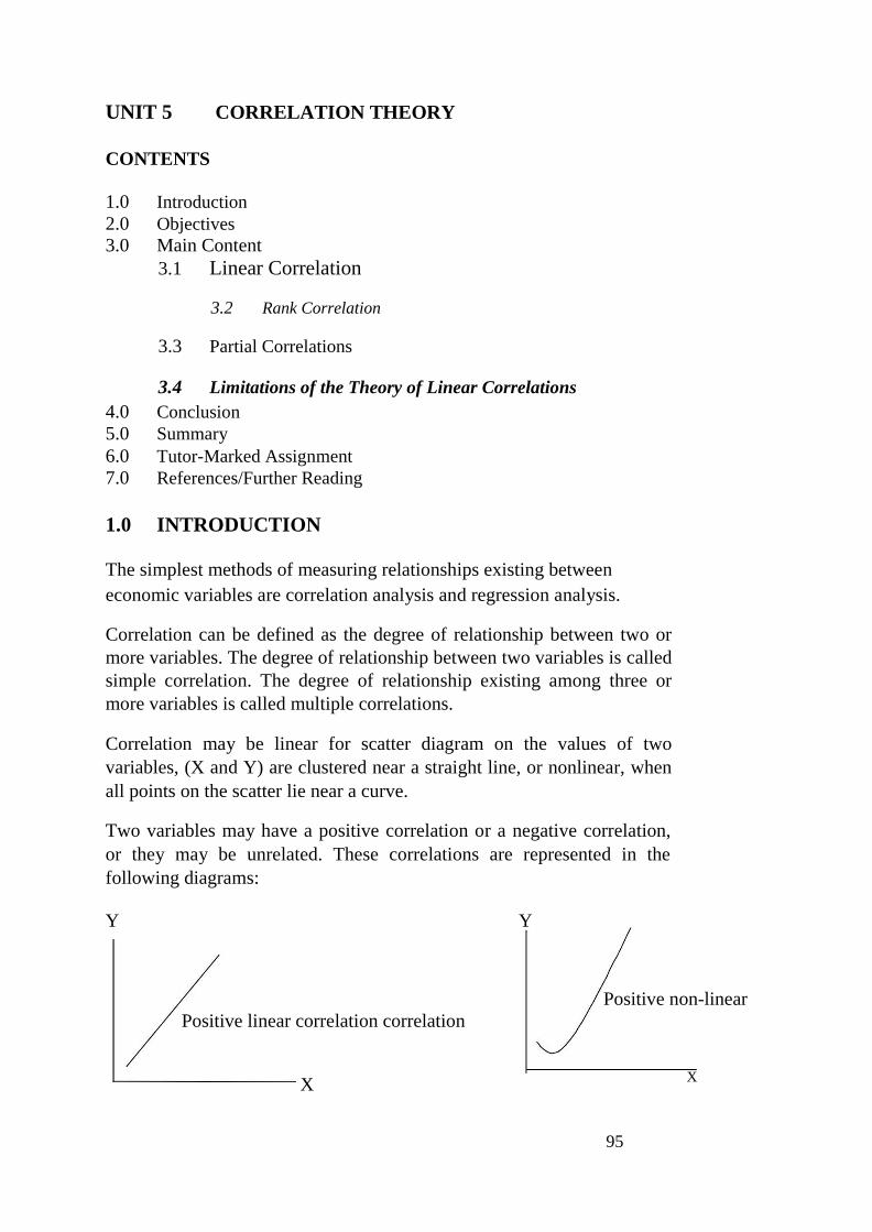
UNIT 5 CORRELATION THEORY

CONTENTS

1.0 Introduction

2.0 Objectives

3.0 Main Content

3.1 Linear Correlation

3.2 Rank Correlation

3.3 Partial Correlations

3.4 Limitations of the Theory of Linear Correlations

4.0 Conclusion

5.0 Summary



1.0 INTRODUCTION

The simplest methods of measuring relationships existing between

economic variables are correlation analysis and regression analysis.

Correlation can be defined as the degree of relationship between two or

more variables. The degree of relationship between two variables is called

simple correlation. The degree of relationship existing among three or

more variables is called multiple correlations.

Correlation may be linear for scatter diagram on the values of two

variables, (X and Y) are clustered near a straight line, or nonlinear, when

all points on the scatter lie near a curve.

Two variables may have a positive correlation or a negative correlation,

or they may be unrelated. These correlations are represented in the

following diagrams:

Y Y

Positive non-linear

Positive linear correlation correlation

X

95

X

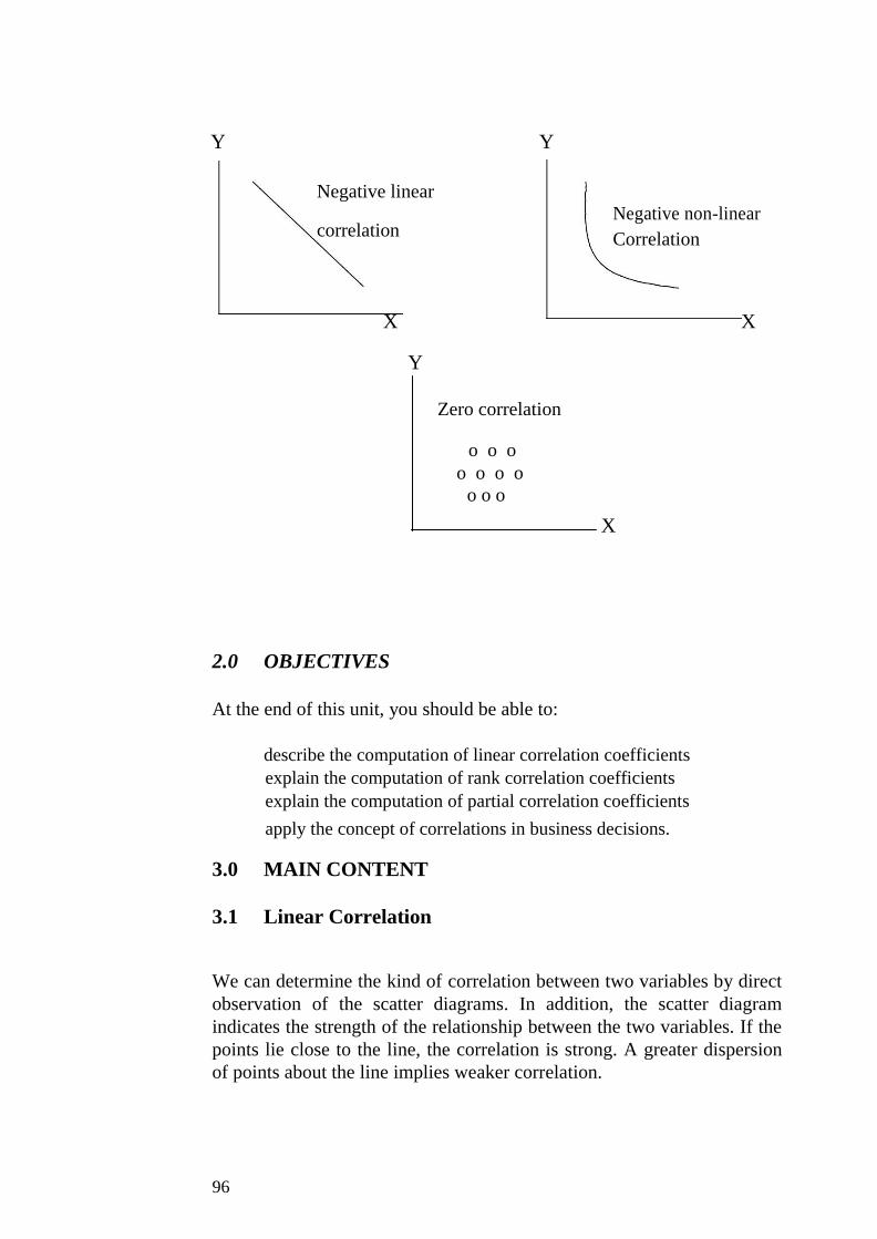
Y Y

Negative linear

Negative non-linear correlation

Correlation

X X

Y

Zero correlation

o o o

o o o o

o o o

X

2.0 OBJECTIVES


describe the computation of linear correlation coefficients

explain the computation of rank correlation coefficients

explain the computation of partial correlation coefficients

apply the concept of correlations in business decisions.

3.0 MAIN CONTENT

3.1 Linear Correlation

We can determine the kind of correlation between two variables by direct

observation of the scatter diagrams. In addition, the scatter diagram

indicates the strength of the relationship between the two variables. If the

points lie close to the line, the correlation is strong. A greater dispersion

of points about the line implies weaker correlation.

96

Note that the inspection of a scatter diagram only gives a rough picture of

the relationship between two variables. For a precise quantitative

measurement of the degree of correlation between two variables, say X

and Y, we use a parameter ⟩ referred to as the correlation coefficient.

The sample estimate of this parameter is referred to as r.

The simple correlation coefficient is computed by:

Example

We want to determine the correlation between Price, X, and quantity

supplied, Y, Given the following data

Time Period (in Quantity supply (Yi) (in Unit Price (Xi) (in

days) tons) Naira)

1 10 2

2 20 4

3 50 6

4 40 8

5 50 10

6 60 12

7 80 14

8 90 16

9 90 18

10 120 20

n = 10 Yi = 610 Xi = 110

= ∑ Xi = 110 = 11,

= ∑Yi = 610 = 61 X Y

10

n 10

n

It can be shown that the formula:

97

= n X i Y i

( X i

)( Y i

)

n X i

2 ( X i )

2 n Yi

2 ( Y i)

2

98

Using the table

X i Yi XiYi X i2

Yi2

2 10 20 4 100

4 20 80 16 400

6 50 300 36 2,500

8 40 320 64 1,600

10 50 500 100 2,500

12 60 720 144 3,600

14 80 1120 196 6,400

16 90 1,440 256 8,100

18 90 1620 324 8100

20 120 2400 400 14400

r = n XiYi ( X i )( Yi )

n X 2 ( X )

2

n Y 2

( Y ) 2

i i 1 i

= 10(8520) (110)(610)

10(1540) (110) 2

10(47700)

(610) 2

= 85200 67100

15400

12100

477000 372100

= 18100

=

18100

(57.45)(323.88)

3300 104900

= 18100

= 0.972 approx.

18606.91

3.3 Rank Correlation

Rank correlation coefficient is used for qualitative variables, whereby

the variables cannot be measured numerically. Examples of such variables

include profession, education, preferences for a particular brand of

commodity and the like.

In such cases, we rank the observations in a specific sequence, such as in

order of size, importance, etc., using numbers 1, 2… n. We therefore,

assign ranks to the data and measure the relationships between their ranks

instead of their actual numerical values.

If two variables, X and Y are ranked, the rank correlation coefficient is

computed by:

rs = 1 – 6 ∑d2

n3 – n

99

Where d2 = [R(X)-R(Y)]

2 = squared difference between ranks

of corresponding pairs of X and Y.

R(X) = individual ranks assigned to X values R(Y) =

individual ranks assigned to Y values n = number of

pairs of observations

There are two important points to note about the rank correlation

coefficient:

1. It does not matter whether the ranking of the observations is in

ascending or descending order.

2. If two or more observations have the same value, we assign to

each observation the Mean rank.

Examples

1. Consider the following table showing how 10 students were ranked

according to their performance in their class work and their final

examinations. Let us find out whether there is a relationship

between the accomplishments of the students during the year and

their performance in their examinations.

Student Ranking Based on Ranking Based on d d2

Class Work Exam. Marks

A 2 1 1 1

B 5 6 -1 1

C 6 4 2 4

D 1 2 -1 1

E 4 3 1 1

F 10 7 3 9

G 7 8 -1 1

H 9 10 -1 1

I 3 5 -2 4 J 8 9 -1 1

d2 = 24

The correlation coefficient in this example is:

rs = 1 – 6 ∑d2 = 1 – 6(24)

n3 – n 103 – 10 = 1 – 0.145 = 0.855

100

The value of rs = 0.855 indicates a close relationship between class work

and examination performance, so that students with good records

throughout the year do well in their examination and vice versa.

2. In a recent research project, a student attempted to find out if the

demand for one specific product is affected by expenditures on

television advertisements.

The following data were obtained from the reference firm:

Year Qd (in Expenditure d d2

thousands) on TV

(Q) Adverts (X)

R(x)-R(Q) {R(x) – R(Q)}2

(N’millions) R(X) R(Q)

1980 35.00 0.05 3.0 3.5 -0.50 0.025

1981 37.50 0.09 7.0 5.0 2.00 4.00

1982 39.20 0.04 1.5 7.0 -5.50 30.25

1983 22.00 0.04 1.5 1.0 0.50 0.25

1984 33.00 0.10 8.5 2.0 6.50 42.25

1985 41.60 0.10 8.5 8.0 0.50 0.25

1986 44.80 0.11 10. 9.0 1.00 1.00

1987 35.00 0.08 6.0 3.5 2.50 6.25

1988 38.00 0.06 4.0 6.0 -2.00 4.00

1989 51.80 0.12 11.0 10.0 1.00 1.00

1990 62.05 0.14 13.0 12.0 1.00 1.00

1991 63.00 0.13 12. 0 13.0 -1.00 1.00

1992 58.30 0.07 5.0 11.0 -6.00 36.00

1993 70.00 0.20 14.0 15.0 -1.00 1.00

1994 68.08 0.21 15.0 14.0 -1.00 1.00

1995 72.00 0.27 16.0 16.0 0.00 0.00

d2=129.50

The rank correlation coefficient can be computed as follows:

rs = 1 – 6 ∑d2 = 1 – 6(129.50)

n3 – n 163 – 16

= 1 – 777 = 0.81

4080

The value, rs = 0.81 indicates a strong positive correlation between the

quantity demanded of the specific product (Q) and expenditure on TV

adverts (X).

10

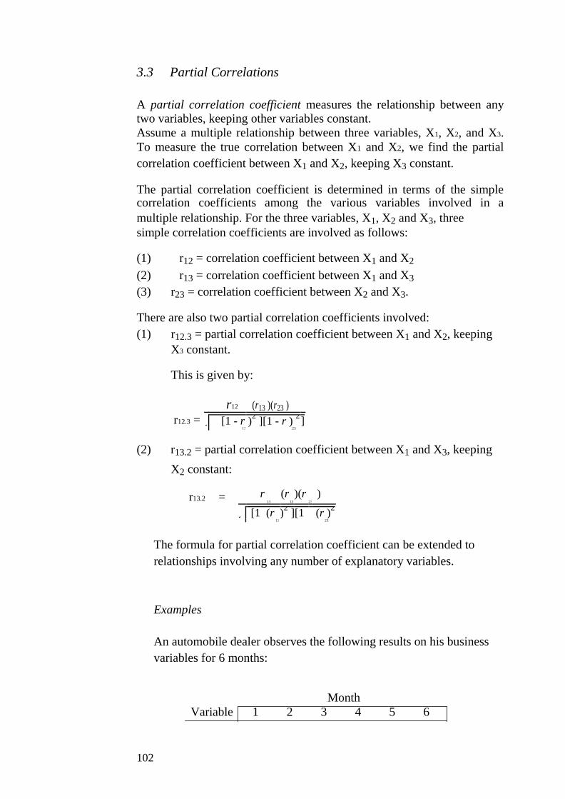
3.3 Partial Correlations

A partial correlation coefficient measures the relationship between any

two variables, keeping other variables constant.

Assume a multiple relationship between three variables, X1, X2, and X3.

To measure the true correlation between X1 and X2, we find the partial

correlation coefficient between X1 and X2, keeping X3 constant.

The partial correlation coefficient is determined in terms of the simple correlation coefficients among the various variables involved in a

multiple relationship. For the three variables, X1, X2 and X3, three

simple correlation coefficients are involved as follows:

(1) r12 = correlation coefficient between X1 and X2 (2) r13 = correlation coefficient between X1 and X3 (3) r23 = correlation coefficient between X2 and X3.

There are also two partial correlation coefficients involved:

(1) r12.3 = partial correlation coefficient between X1 and X2, keeping

X3 constant.

This is given by:

r12.3 =

r12 (r13 )(r23 )

[1 - r )2 ][1 - r )

2 ]

13 23

(2) r13.2 = partial correlation coefficient between X1 and X3, keeping

X2 constant:

r13.2 = r (r )(r ) 13 13 23

[1 (r )2 ][1 (r )

2

13 23

The formula for partial correlation coefficient can be extended to

relationships involving any number of explanatory variables.

Examples

An automobile dealer observes the following results on his business

variables for 6 months:

Month

Variable 1 2 3 4 5 6

102

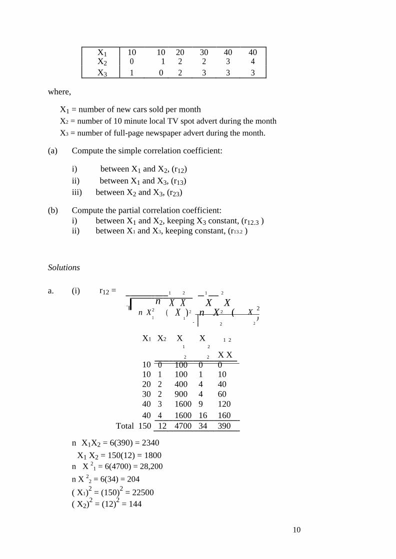
X1 10 10 20 30 40 40 X2 0 1 2 2 3 4

X3 1 0 2 3 3 3

where,

X1 = number of new cars sold per month

X2 = number of 10 minute local TV spot advert during the month

X3 = number of full-page newspaper advert during the month.

(a) Compute the simple correlation coefficient:

i) between X1 and X2, (r12) ii) between X1 and X3, (r13)

iii) between X2 and X3, (r23) (b) Compute the partial correlation coefficient:

i) between X1 and X2, keeping X3 constant, (r12.3 )

ii) between X1 and X3, keeping constant, (r13.2 )

Solutions

a. (i) r12 = 1 2 1 2

n X 2

n (

X X

X) 2 n

X X 2

X ( X

2

1

1

2

)

X1

X2

X

X

2

1 2 1 2

X X

2 2

10

0 100 0 0

10 1 100 1 10

20 2 400 4 40

30 2 900 4 60

40 3 1600 9 120

40 4 1600 16 160

Total 150 12 4700 34 390

n X1X2 = 6(390) = 2340

X1 X2 = 150(12) = 1800

n X 21 = 6(4700) = 28,200

n X 22 = 6(34) = 204

( X1)2 = (150)

2 = 22500

( X2)2 = (12)

2 = 144

10

r12 =

2340 - 1800

28200 - 22500 204 144

= 540 (75.4983)(7.7460)

= 540 584.81 = 0.923

This implies a very close relationship between the number of cars sold per

month and the number of 10-minute local TV spot adverts during the

month.

a.(ii) r13 = 1 3 1 2

X n X X X X 1 ( X1 ) n X3 ( X3 )

2

2 2 2

Using the table below:

X1 X3 X X 1 3

2 3 X X 2 2

10 1 100 1 10

10 0 100 0 0

20 2 400 4 40

30 3 900 9 90

40 3 1600 9 120

40 3 1600 9 120

TOTAL 150 12 4700 32 380

n X1X3 = 6(380) = 2280

X1 X3 = 150(12) = 1800

n X12

= 6(4700) = 28200

n X32

= 6(32) = 192

( X1)2

= (150)2 = 22500

( X3)2

= (12)2 = 144

r13 = 2280 - 1800

28200 - 22500 192 144

= 480

(75.4983)(6.9282)

= 480 523.0673 = 0.918

104

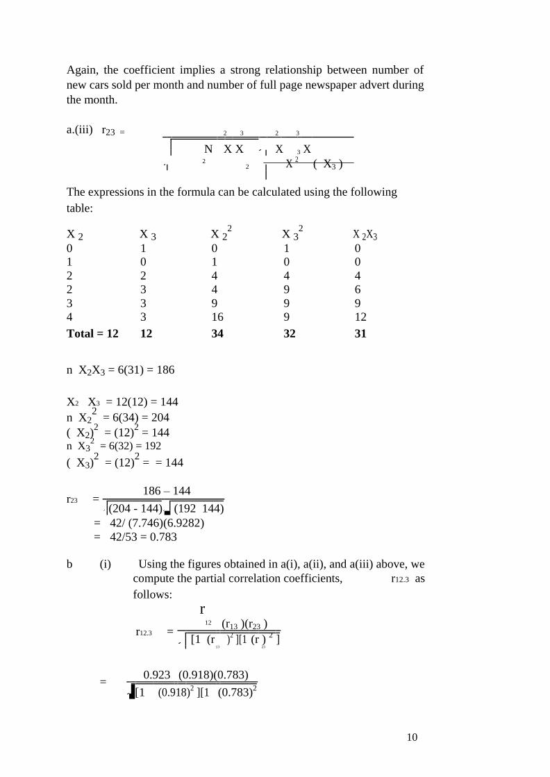
Again, the coefficient implies a strong relationship between number of

new cars sold per month and number of full page newspaper advert during

the month.

a.(iii) r23 = 2 3 2 3

N X X X 3 X

2 2

X 2 ( X3 )

The expressions in the formula can be calculated using the following

table:

X 2 X 3 X 22

X 32

X 2X3

0 1 0 1 0 1 0 1 0 0

2 2 4 4 4

2 3 4 9 6

3 3 9 9 9

4 3 16 9 12

Total = 12 12 34 32 31

n X2X3 = 6(31) = 186

X2 X3 = 12(12) = 144

n X22 = 6(34) = 204

( X2)2 = (12)

2 = 144

n X32 = 6(32) = 192

( X3)2 = (12)

2 = = 144

r23 = 186 – 144

(204 - 144)

(192 144)

= 42/ (7.746)(6.9282) = 42/53 = 0.783

b (i) Using the figures obtained in a(i), a(ii), and a(iii) above, we

compute the partial correlation coefficients, r12.3 as

follows:

r12.3 =

r12 (r13 )(r23 )

[1 (r

)2 ][1 (r )

2 ]

13 23

=

0.923 (0.918)(0.783)

[1 (0.918)2 ][1 (0.783)

2

10

= 0.923 0.7188

(0.1573)(0.3869)

= 0.2042

(0.6082

= 0.2042/0.2467 = 0.8277

It follows that the partial correlation between the number of new cars sold

per month, X1, and the number of 10-minute local TV spot advert

during the month, X2, keeping the number of full-page advert, X3,

constant is high.

b (ii) The partial correlation between the number of new cars sold per month and the number of full-page newspaper advert during the month,

keeping the number of 10-minute advert during the month, r13.2, can be

similarly obtained as follows:

r13.2 = r13 (r12 )(r23 )

[1 (r )2 ][1 (r )

2 ]

12 23

=

0.918 (0.923)(0.783)

[1 (0.923)2 ][1

(0.783)2 ]

=

0.1953

(0.1489)(0.3869)

= 0.1953/0.2400 = 0.8138

The computed coefficient indicates a high partial correlation between the

number of new cars sold and the number of full-page advert during the

month, keeping the number of 10-minute spot advert constant.

3.4 Limitations of the Theory of Linear Correlations

The limitations of linear correlations as a technique for the study of

economic relations are as follows:

1. The formula for correlation coefficient applies only to linear relationships between variables.

2. That correlation coefficient is a measure of co-variability of

variables does not imply any functional relationship between the

variables concerned.

106


1. How does simple correlation differ from partial correlation? 2. Use graphs to illustrate: positive linear correlation, negative

nonlinear correlation, and zero correlation between two variables

10

4.0 CONCLUSION

The relationships among business variables can simply be identified using

correlation coefficients. Two variables can either be positively or

negatively correlated. This correlation can be linear or nonlinear

depending on variable characteristics.

Three basic types of correlations were discussed in this unit: (i) the simple

linear correlation; (ii) rank correlation; and, (iii) partial correlation. You

should note that partial correlations involve more than two different

variables. Here, the correlation between two identified variables, are

obtained holding other variables constant.

5.0 SUMMARY

For a precise quantitative measurement of the degree of correlation

between two variables, say X and Y, we use a parameter ⟩ referred to as

the correlation coefficient. The sample estimate of this parameter is

referred to as r.

Rank Correlation Coefficient is used for qualitative variables, whereby

the variables cannot be measured numerically. Examples of such variables

include profession, education, preferences for a particular brand of

commodity and the like.

A partial correlation coefficient measures the relationship between any

two variables, keeping other variables constant.

The limitations of linear correlations as a technique for the study of

economic relations are as follows:

1. The formula for correlation coefficient applies only to linear

relationships between variables.

2. That correlation coefficient as a measure of co-variability of

variables does not imply any functional relationship between the

variables concerned.


The following data give the actual sales of a company in each of 8 States

of a hypothetical country, together with the forecast of sales by two

different methods:

108

State Actual Sales Forecast 1 Forecast 2

(N’million)

A 15 13 16 B 19 25 19

C 30 23 26

D 12 26 14

E 58 48 65

F 10 15 19

G 23 28 27

H 17 10 22

(a) Calculate the rank correlation coefficient between: (i) actual sales and forecast 1 (ii) actual sales and forecast 2

(b) Which forecasting method would you recommend next year and

why?



edition.


10

MODULE 3

Unit 1 Forecasting and Time-Series Analysis

Unit 2 Index Numbers

Unit 3 Inventory Control

Unit 4 Decision Analysis

Unit 5 Network Planning and Analysis

UNIT 1 FORECASTING AND TIME-SERIES ANALYSIS

CONTENTS

1.0 Introduction

2.0 Objectives

3.0 Main Content

3.1 Steps in Forecasting

3.2 Types of Forecasts

3.3 Forecasting Techniques

3.3.1 Moving Averages

3.3.2 Least Squares or Trend Lines

4.0 Conclusion

5.0 Summary



1.0 INTRODUCTION

Forecasts are based on past performances. In other words, future values

are predicted from past values. This assumes that the future will be

basically the same as the past and present, implying that the relationships

underlying the phenomenon of interest are stable overtime.

Forecasting can be performed at different levels, depending on the use to

which it will be put. Simple guessing, based on previous figures, is

occasionally adequate. However, where there is a large investment at

stake, structured forecasting is essential.

Any forecasts made, however technical or structured should be treated

with caution, since the analysis is based on past data and there could be

unknown factors present in the future. However it is often reasonable to

assume that patterns that have been identified in the analysis of past data

will be broadly continued, at least into the short-term future.

110

2.0 OBJECTIVES


list the necessary steps in forecasting activities

enumerate the different types of forecasting

apply the basic forecasting techniques.

3.0 MAIN CONTENT

3.1 Steps in Forecasting

We outline the basic steps in forecasting as follows:

Step 1 Gather past data: daily, weekly, monthly and yearly.

Step 2 Adjust or clean up the raw data against inflationary

factors. Index numbers can be used in deflating

Step 3

inflationary factors.

Make forecasts from the “refined” data

Step 4 When the future data (which is been forecast) becomes

available, compare forecasts with actual values, by so

doing, you will be able to establish the error due to

forecasting.

3.2 Types of Forecasts

The basic types of forecasts are outlined below:

1. Short-term forecasts: these are forecasts concerning the near

future. They, are characterised by few uncertainties and therefore

more accurate then distant future forecasts

2. Long – term forecasts: these concern the distant future. They are

characterised by more uncertainties than short – term forecasts.

3. Extrapolation: these are forecasts based solely on past and present

values of the variable to be forecast. In this case, future values are

extrapolated from past and present values. 4. Forecasts based on established relationships between the variable

to be forecast and other variables.

3.3 Forecasting Techniques

The two generally used methods of forecasting include:

1. moving averages 2. trend lines or least squares.

111

3.3.1 Moving Averages

Moving averages can be used to generate the general picture (or trend)

behind a set of data or time series. The general pattern generated can be

used to forecast future values.

Note that a time series is a name given to numerical data described over a

uniform set of time points. Time series occur naturally in all spheres of

business activity.

The method of moving averages can be illustrated by the following

example.

A monthly sales data is given:

Sales (N) Jan Feb March April May June

Past (Actual) 50 55 70 50 45 90

Using a 3 – period moving averages, the forecast values are:

50 + 55 + 70

= 58 (Feb) 3

55 + 70 + 50

= 58 (March) 3

70 + 50 + 45

= 55 (April) 3

50 + 55 + 70

= 58 (May) 3

We can thus summarise the forecast sales as follows:

Forecast sales (N) Jan Feb March April May June

Future (forecast) - 58 58 55 62 -

These can be presented in a graph as in figure 11.1 below:

112

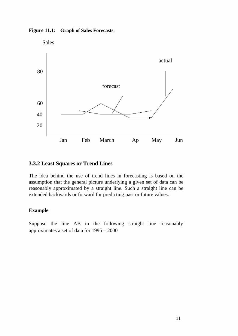
Figure 11.1: Graph of Sales Forecasts.

Sales

actual

80

forecast

60

40

20

Jan Feb March Ap May Jun

3.3.2 Least Squares or Trend Lines

The idea behind the use of trend lines in forecasting is based on the

assumption that the general picture underlying a given set of data can be

reasonably approximated by a straight line. Such a straight line can be

extended backwards or forward for predicting past or future values.

Example

Suppose the line AB in the following straight line reasonably

approximates a set of data for 1995 – 2000

11

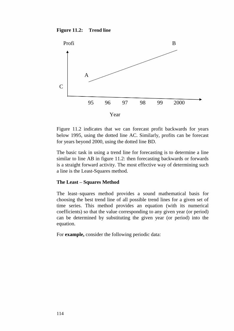
Figure 11.2: Trend line

Profi B

A

C

95 96 97 98 99 2000

Year

Figure 11.2 indicates that we can forecast profit backwards for years

below 1995, using the dotted line AC. Similarly, profits can be forecast

for years beyond 2000, using the dotted line BD.

The basic task in using a trend line for forecasting is to determine a line

similar to line AB in figure 11.2: then forecasting backwards or forwards

is a straight forward activity. The most effective way of determining such

a line is the Least-Squares method.

The Least – Squares Method

The least–squares method provides a sound mathematical basis for

choosing the best trend line of all possible trend lines for a given set of

time series. This method provides an equation (with its numerical

coefficients) so that the value corresponding to any given year (or period)

can be determined by substituting the given year (or period) into the

equation.

For example, consider the following periodic data:

114

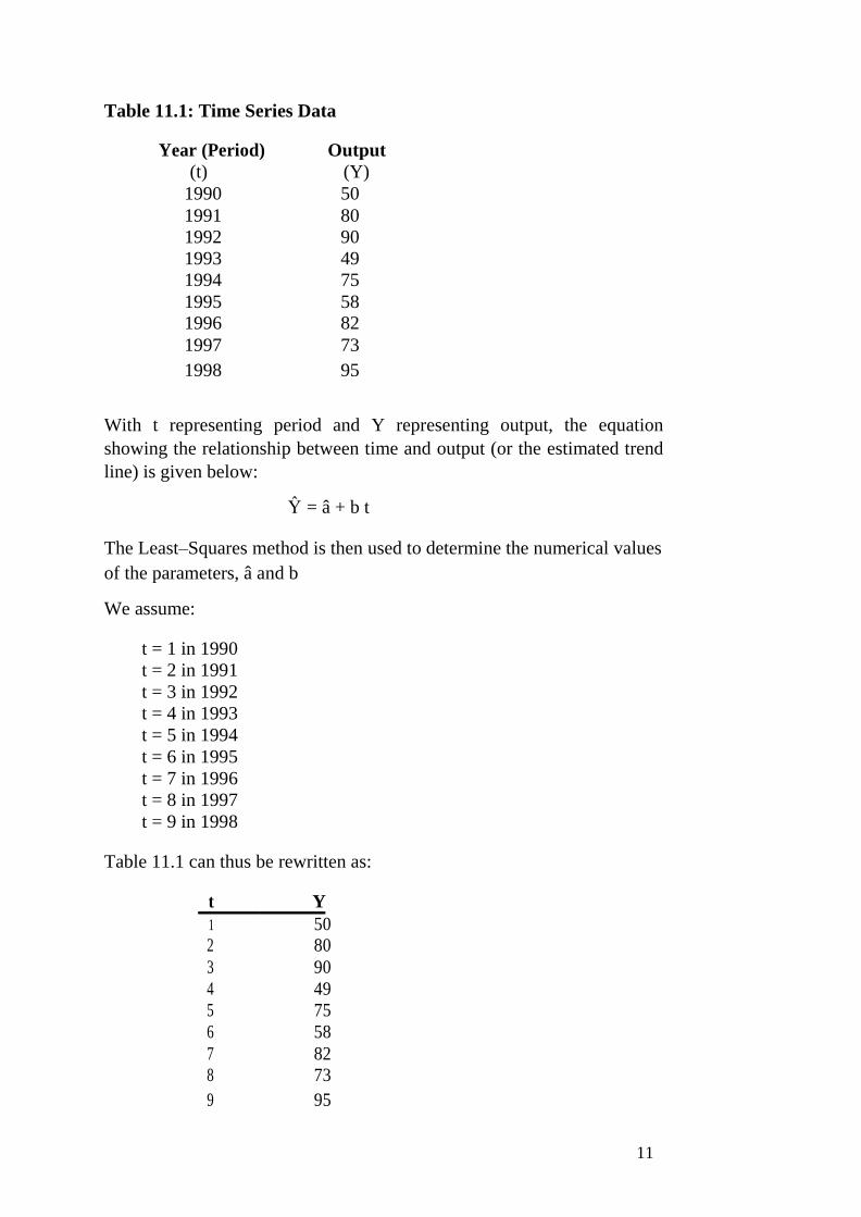
Table 11.1: Time Series Data

Year (Period) Output

(t) (Y)

1990 50

1991 80

1992 90

1993 49

1994 75

1995 58 1996 82

1997 73

1998 95

With t representing period and Y representing output, the equation

showing the relationship between time and output (or the estimated trend

line) is given below:

Ŷ = â + b t

The Least–Squares method is then used to determine the numerical values

of the parameters, â and b

We assume:

t = 1 in 1990

t = 2 in 1991

t = 3 in 1992

t = 4 in 1993

t = 5 in 1994

t = 6 in 1995

t = 7 in 1996

t = 8 in 1997

t = 9 in 1998

Table 11.1 can thus be rewritten as:

t Y

1 50 2 80

3 90

4 49

5 75

6 58

7 82

8 73

9 95

11

The formulas for the least – squares estimates are as follows:

ˆ

â =

Y

- b t

Where

=

;

= t ; n = number of pairs of observations Y Y t

n n

ˆ n tY - t Y

b =

n

t

2 (

t)2

Using the given data and second formula, we get:

t Y tY t 2

1 50 50 1

2 80 160 4

3 90 270 9

4 49 196 16

5 75 375 25

6 58 348 36

7 82 574 49

8 73 584 64

9 95 855 81

45 652 3412 285_

Thus, n tY = 9(3412) = 30708

t Y = 45(652) = 29340

n t2 = 9(285) = 2565

(n t)2 = (45)

2 = 2025

= Y

= 652

= 72.44

y

n

9

= t

= 45 = 5

t

9

It follows that: n

30708 29340

=

1368

= 25.53

b =

2562 - 2025 540

116

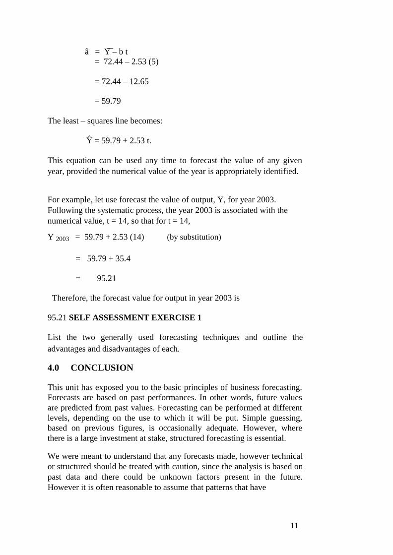
â = Y – b t = 72.44 – 2.53 (5)

= 72.44 – 12.65

= 59.79

The least – squares line becomes:

Ŷ = 59.79 + 2.53 t.

This equation can be used any time to forecast the value of any given

year, provided the numerical value of the year is appropriately identified.

For example, let use forecast the value of output, Y, for year 2003.

Following the systematic process, the year 2003 is associated with the

numerical value, t = 14, so that for t = 14,

Y 2003 = 59.79 + 2.53 (14) (by substitution)

= 59.79 + 35.4

= 95.21

Therefore, the forecast value for output in year 2003 is

95.21 SELF ASSESSMENT EXERCISE 1

List the two generally used forecasting techniques and outline the

advantages and disadvantages of each.

4.0 CONCLUSION

This unit has exposed you to the basic principles of business forecasting.

Forecasts are based on past performances. In other words, future values

are predicted from past values. Forecasting can be performed at different

levels, depending on the use to which it will be put. Simple guessing,

based on previous figures, is occasionally adequate. However, where

there is a large investment at stake, structured forecasting is essential.

We were meant to understand that any forecasts made, however technical

or structured should be treated with caution, since the analysis is based on

past data and there could be unknown factors present in the future.

However it is often reasonable to assume that patterns that have

11

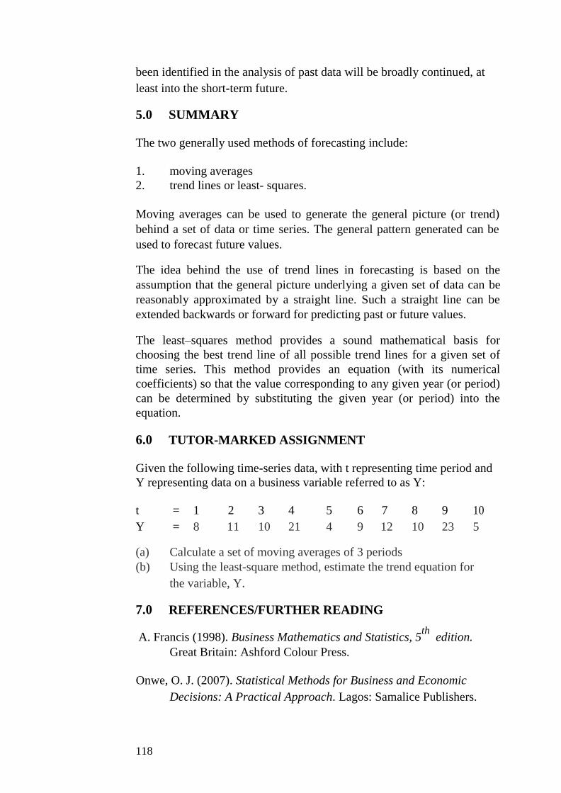
been identified in the analysis of past data will be broadly continued, at

least into the short-term future.

5.0 SUMMARY

The two generally used methods of forecasting include:

1. moving averages 2. trend lines or least- squares.

Moving averages can be used to generate the general picture (or trend)

behind a set of data or time series. The general pattern generated can be

used to forecast future values.

The idea behind the use of trend lines in forecasting is based on the

assumption that the general picture underlying a given set of data can be

reasonably approximated by a straight line. Such a straight line can be

extended backwards or forward for predicting past or future values.

The least–squares method provides a sound mathematical basis for

choosing the best trend line of all possible trend lines for a given set of

time series. This method provides an equation (with its numerical

coefficients) so that the value corresponding to any given year (or period)

can be determined by substituting the given year (or period) into the

equation.


Given the following time-series data, with t representing time period and

Y representing data on a business variable referred to as Y:

t = 1 2 3 4 5 6 7 8 9 10

Y = 8 11 10 21 4 9 12 10 23 5

(a) Calculate a set of moving averages of 3 periods (b) Using the least-square method, estimate the trend equation for

the variable, Y.



edition.


Onwe, O. J. (2007). Statistical Methods for Business and Economic

Decisions: A Practical Approach. Lagos: Samalice Publishers.

118

UNIT 2 INDEX NUMBERS

CONTENTS

1.0 Introduction

2.0 Objectives

3.0 Main Content

3.1 Index Relatives

3.2 The Simple Aggregate Price Index

3.3 Weighted Aggregate Price Index

3.4 The Laspeyres and Paasche Indices

3.5 Comparing Laspeyres with Paasche Price Indices

3.6 Uses and Limitations of Index Numbers

3.6.1 Uses of Index Numbers

3.6.2 Limitations of Index Numbers

4.0 Conclusion

5.0 Summary



1.0 INTRODUCTION

Index numbers are often used in stabilising the time value of money and

in deflating nominal values. An index number measures the percentage

change in the value of some economic commodity over a period of time.

Index numbers are expressed in terms of a base of 100. Economic

commodity is a term used to describe anything measurable and has some

economic relevance. Examples include price, wage quantity, productivity,

expenditure, and the like.

Two or more time periods are usually involved in the computation of an

index number. One of these time periods represents the base time period.

The value of the base time period stands as the standard point of

comparison, while the values at the other time periods are used to show

the percentage in value from the standard value of the base period.

Examples

1. Suppose we wish to compare the average monthly salaries of

workers in a given company for:

1985, 1990, 1995, 2000, 2005 and 2010, using 1985 as the base

year. The salary index for each of the six years can be calculated

using the following relationship:

11

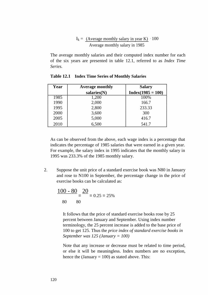
Ik = (Average monthly salary in year K) ⋅100

Average monthly salary in 1985

The average monthly salaries and their computed index number for each

of the six years are presented in table 12.1, referred to as Index Time

Series.

Table 12.1 Index Time Series of Monthly Salaries

Year Average monthly Salary

salaries(N) Index(1985 = 100) 1985 1,200 100% 1990 2,000 166.7

1995 2,800 233.33

2000 3,600 300

2005 5,000 416.7

2010 6,500 541.7

As can be observed from the above, each wage index is a percentage that

indicates the percentage of 1985 salaries that were earned in a given year.

For example, the salary index in 1995 indicates that the monthly salary in

1995 was 233.3% of the 1985 monthly salary.

2. Suppose the unit price of a standard exercise book was N80 in January

and rose to N100 in September, the percentage change in the price of

exercise books can be calculated as:

100 - 80 =

20 = 0.25 = 25%

80 80

It follows that the price of standard exercise books rose by 25

percent between January and September. Using index number

terminology, the 25 percent increase is added to the base price of

100 to get 125. Thus the price index of standard exercise books in

September was 125 (January = 100)

Note that any increase or decrease must be related to time period,

or else it will be meaningless. Index numbers are no exception,

hence the (January = 100) as stated above. This:

120

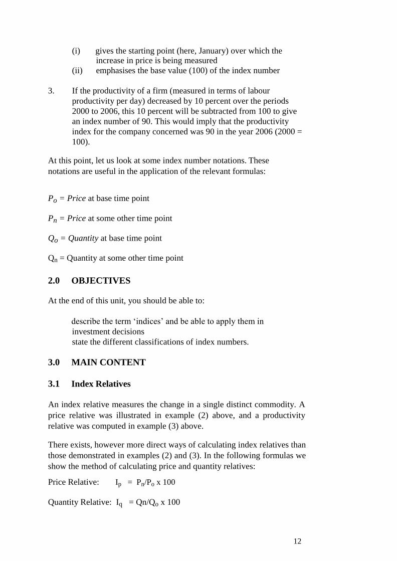
(i) gives the starting point (here, January) over which the increase in price is being measured

(ii) emphasises the base value (100) of the index number

3. If the productivity of a firm (measured in terms of labour

productivity per day) decreased by 10 percent over the periods

2000 to 2006, this 10 percent will be subtracted from 100 to give

an index number of 90. This would imply that the productivity

index for the company concerned was 90 in the year 2006 (2000 =

100).

At this point, let us look at some index number notations. These

notations are useful in the application of the relevant formulas:

Po = Price at base time point

Pn = Price at some other time point

Qo = Quantity at base time point

Qn = Quantity at some other time point

2.0 OBJECTIVES


describe the term ‘indices’ and be able to apply them in

investment decisions

state the different classifications of index numbers.

3.0 MAIN CONTENT

3.1 Index Relatives

An index relative measures the change in a single distinct commodity. A

price relative was illustrated in example (2) above, and a productivity

relative was computed in example (3) above.

There exists, however more direct ways of calculating index relatives than

those demonstrated in examples (2) and (3). In the following formulas we

show the method of calculating price and quantity relatives:

Price Relative: Ip = Pn/Po x 100

Quantity Relative: Iq = Qn/Qo x 100

12

Examples

Table 12.2 below gives details of price and quantities sold of two items

(Video and Television) in a particular Cash and Carry Merchandise store

over two years (2007 and 2008)

Table 12.2 Price and Quantity Relatives for 2008

2007 2008

Item Price Quantity Price Quantity

Video Recorder Po Qo Pn Qn

N12,500 40 N12,700 25

Television N30,000 28 N32,000 40

You are required to calculate the price and quantity relatives for both

items for the year 2008 (2007 = 100)

Video:

∑Pn

12,700

Price Relative = Ivp = ⋅100 = ⋅ 100 = 101.60

∑P 12,500

O

Quantity Relative = Ivq = ∑Qn ⋅100 = 25 ⋅100 = 62.50

∑Qo 40

Television:

Price Relative = Itp = ∑Pn .100 = 32,000 .100 = 106.67

∑Po 30,000

Quantity Relative = Itq = ∑Qn/Qo x 100 = 40/28 x 100 = 142.86

3.3 The Simple Aggregate Price Index

The Simple Price Index can be defined as the ratio of the sum of

commodity prices in a given current period to the sum of same

commodity prices in the selected base year (or period).

Symbolically,

Simple Price Index, PI = ∑Pn

⋅ 100,

∑Po

122

Where Pn = current year’s prices.

Po = base year’s prices.

Note that, given the Quantity Index (QI) defined by:

QI = ∑Q n ⋅100

∑Q o

The corresponding Value Index (VI) is computed by:

VI = ∑Pn Qn ⋅ 100

∑Po Qo

The simple aggregate price index is commonly used in comparing two

sets of prices from a wide variety of items.

Example:

The average consumer prices, in naira per Kg, for some staple food items

in 2000 and 2006 are given in the following table 12.3. We are required to

find the Aggregate Price Index for 2006, using 2000 as the base year.

Table 12.3 Average Consumer Prices for Selected Staple Food

Items

Item 2000 2006

Sugar 10 40

Wheat Flour 11 20

Butter 71 99

Ground beef 91 186

Frying Chicken 39 88

Solution:

The required aggregate price index for 2006 is:

12

40 + 20 + 99 + 186 + 88

=

433

⋅100 I2006 =

10 + 11 + 71 + 91 + 39 222

= 195.06

This implies that the prices of the five items are higher by 95.06 percent

in 2006 than in 2000.

3.4 Weighted Aggregate Price Index

The weighted aggregate price index is the ratio of an aggregate of

weighted commodity prices for a given year, K, to an aggregate of the

weighted prices of the same commodities in some base year, expressed as

a percentage.

Symbolically,

Ik = ∑ i = 1Pki qki x 100 n

i =1Poi qoi

Example:

An investor’s holding in the shares of four companies in 2004 and 2006

is shown in Table 12.4 below:

Table 12.4 Investor’s Holding of Four Companies

No of shares Price per share ( N )

Company 2004 2006 2004 2006 A 350 400 0.50 1.25 B 200 180 1.25 3.75

C 140 200 6.25 12.50

D 130 150 12.50 18.75

Using 2004 as base year, calculate:

(a) a simple aggregate price index and (b) a weighted aggregate price index for the investor’s holding of

shares.

Solutions:

(a) The simple aggregate index is:

Ip2006 = ∑ P 2006 ⋅100 = 400 + 180 + 200 + 150 ⋅100

350 + 200 + 140 + 130 ∑P2004

= 1.134 x 100

= 113.4

124

i

n

(b) The weighted aggregate price index is:

Iwp 2006 = ∑ P2006 Q2006

⋅100

∑P2004 Q2004

= 1.25(400) + 3.75(180) + 12.50(200) + 18.75(150) ⋅100

0.50(350) + 1.25(200) + 6.25(140) + 12.5(130)

= 500 + 675 + 2500 + 281.5 ⋅100

175 + 250 + 875 + 1625

= 6487

2925.5

= 2.218 ⋅100

= 221.79

3.4 The Laspeyres and Paasche Indices

A Laspeyres index is a special case of weighted aggregate index. This

index uses base time period weights. It is usually associated with price

and quantity indices where:

A Laspeyres Price Index uses base time period quantities as weights

A Laspeyres Quantity Index uses base time period prices as weights

The formulae for calculating a Laspeyres Index is derived from the

general formula for weighted aggregate index. The commonly use

formulae are as follows:

1. Price Index = Lp = ∑Pn Qo .100 ∑Po Qo

2. Quantity Index = Lq = ∑Po Qo .100 ∑Po Qo

The Paasche Indices

The Paasche index is another special case of weighted aggregate indices.

It uses current time period weights, and is most commonly associated

with price and quantity indices, where:

A Paasche Price Index uses current time period quantities as weights

A Paasche Quantity Index uses current time period prices as weights.

As with the Laspeyres index, the formulae most commonly used for

calculating a Paasche Index is given as:

12

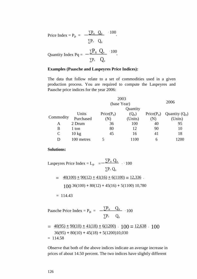
Price Index = Pp = ∑Pn Qn ⋅100

∑Po Qn

Quantity Index Pq = ∑Pn Qn ⋅100

∑Pn Qo

Examples (Paasche and Laspeyres Price Indices):

The data that follow relate to a set of commodities used in a given

production process. You are required to compute the Laspeyres and

Paasche price indices for the year 2006:

2003 2006 (base Year)

Commodity Units Price(Po)

Quantity

(Qo) Price(Po) Quantity (Qo)

Purchased (N) (Units) (N) (Units)

A 2 Drum 36 100 40 95

B 1 ton 80 12 90 10

C 10 kg 45 16 41 18

D 100 metres 5 1100 6 1200

Solutions:

Laspeyres Price Index = Lp = ∑Pn Qo ⋅100

∑Po Qo

= 40(100) + 90(12) + 41(16) + 6(1100) = 12,336 ⋅

100 36(100) + 80(12) + 45(16) + 5(1100) 10,780

= 114.43

Paasche Price Index = Pp = ∑Pn Qn ⋅100

∑Po Qn

= 40(95) + 90(10) + 41(18) + 6(1200) ⋅ 100 = 12,638 ⋅ 100

36(95) + 80(10) + 45(18) + 5(1200)10,030

= 114.58

Observe that both of the above indices indicate an average increase in

prices of about 14.50 percent. The two indices have slightly different

126

values because of the differences in the weights used for the

commodities.

12

3.5 Comparing Laspeyres with Paasche Price Indices

What the Indices are supposed to calculate.

Laspeyres: This compares base period expenditure with a hypothetical

current period expenditure at base period quantities.

Paasche: compares current period expenditure with a hypothetical base

period expenditure at current period quantities when prices are rising.

Laspeyres Index tends to over-estimate price increases and the Paasche

index tends to under-estimate price increases. These are often looked at

as disadvantages for these indices.

Nature of the Indices

The Laspeyres Index is thought of as a ‘pure’ price index as it compares

like with like from period to period. The Paasche Index is not considered

as ‘pure’ price index since the weights change from period to period and

like is not compared with like. This is the major disadvantage of the

Paasche index.

Weights used in calculations

Since the Laspeyres index uses base period quantities as weights, the

index can be outdated. Paasche index uses current quantities as weights

and hence it is always up-to-date.

Ease of calculation

The Laspeyres index needs only the base period quantities, no matter the

number of periods. The Paasche index needs new quantities for each time

period.

3.6 Uses and Limitations of Index Numbers

3.6.1 Uses of Index Numbers

Index numbers are mostly used to reflect changes in general economic

conditions over identified period of time. For instance, the Retail Price

Index (RTI) measures changes in the cost of living; the Index of Industrial

Production reflects changes in industrial output; the Ordinary Share Index

reflects the general state of the Stock Market.

128

Index numbers are used by policy makers to decide on tax changes,

subsidies to parastatals, industries, and so on. Trade Unions use national

cost of living and production indices in negotiating for wages or in

comparing the cost of living across national boundaries, states, or

professions. Insurance companies use various cost indices to index-link

house policies.

Other uses of index numbers include:

1. Determination of real economic values

In periods of inflation, the actual value of a commodity does not serve as

the best guide of its real value (or worth). The worth of any commodity

can only be measured relative to the value of associated commodities.

Some relevant indicator (such as index number) against which to judge

value is necessary.

Example

Suppose the annual rent of some business shops last year was N250, 000,

and this year it has been increased by 10 percent to N275, 000. You can

observe that the actual cost is higher. If we obtain some information that

the cost of business shops in the state as a whole has risen by 15 percent

over the past year, you can rightly argue that the real cost of the given

shops has decreased. But if business turnover for the shops (as an

alternate indicator) has only increased by 5 percent, you may argue that

the real cost of the shops has increased. It follows that, depending on the

particular indicator chosen, the real value of a commodity can change.

There are two major types of standard national indicators. These include:

rate of inflation (often represented by the Retail Price Index), and the

Index of Output of the Production industry.

2. Time-Series Deflation

Time-series deflation is used to obtain a set of index relatives that

measure changes in the real value of some commodities with respect to

some given indicators. In general, given a time-series with x-values, and

some indicator index series with I-values for comparison, the Real Value

Index (RVI) for period n is determined by:

RVI = Current Value (x n ) ⋅ Base Indicator (Io ) ⋅100

Base Value (x o ) Current Indicator (In )

12

= x

n ⋅

Io ⋅ 100

x o In

Example:

The following table presents the values of the average daily wages (N)

and Relative Price Index for eight months. You are required to compute

the monthly real wage indices.

Month 1 2 3 4 5 6 7 8 Daily 17.60 18.10 18.90 19.60 20.25 20.30 20.60 21.40

Wage (N)

Retail 106.1 107.9 112.0 113.1 116.0 117.4 119.5 119.7 Price

Index

Real Wage Index for Month 1(Base Period):

17.60 ⋅ 106.1 ⋅ 100 = 100

17.60 106.1

Real Wage Index for Month 2:

18.10 ⋅

106.1 ⋅ 100 = 100.94

17.60 107.9


18.90 ⋅

106.1 ⋅ 100 = 102.03

17.60 112.0


19.60 . 106.1 . 100 = 106.6 17.60 113.1


20.25 . 106.1 . 100 = 105.3

17.60 116.0

130


20.30 ⋅ 106.1

⋅ 100 = 104.2

17.60 117.4


20.60 ⋅ 106.1

⋅100 = 104.2

17.60 119.5


21.40 ⋅

106.1 ⋅100 = 108.2

17.60 119.7

The last real wage index indicates that the average daily wage had

increased by 8.2 percent over the eight-month period. In real terms,

wages increased steadily, except for months 6 and 7.

3.6.2 Limitations of Index Numbers

The limitations include, among others:

1. Indices give only general view about economic changes over wide

geographical areas. It follows that they will not generally cater for

minority groups or professions, or measure regional variations. For

instance, an individual’s food bill for a particular month may have

increased significantly even though the food index or Retail Price

Index for that month may have shown a decrease.

2. Weighting factors can become out-dated, thus the index may fail to

compare ‘like with like’. 3. If samples were used to obtain data for either values or weights,

the information obtained might be biased, incomplete or false. 4. Index numbers can be misinterpreted by uninformed laypersons.


Outline the uses of index numbers in business and economic decisions.

13

4.0 CONCLUSION

Index numbers are often used in stabilising the time value of money and

in deflating nominal values. An index number measures the percentage

change in the value of some economic commodity over a period of time.

Index numbers are expressed in terms of a base of 100. Economic

commodity is a term used to describe anything measurable and has some

economic relevance. Examples include price, wage quantity, productivity,

expenditure, and the like.

Two or more time periods are usually involved in the computation of an

index number. One of these time periods represents the base time period.

The value of the base time period stands as the standard point of

comparison, while the values at the other time periods are used to show

the percentage in value from the standard value of the base period.

5.0 SUMMARY

The Simple Price Index can be defined as the ratio of the sum of

commodity prices in a given current period to the sum of same

commodity prices in the selected base year (or period).

The weighted aggregate price index is the ratio of an aggregate of

weighted commodity prices for a given year, K, to an aggregate of the

weighted prices of the same commodities in some base year, expressed as

a percentage.

Symbolically,

Ik = n i = 1Pki qki x 100

n

i =1Poi qoi

A Laspeyres index is a special case of weighted aggregate index. This

index uses base time period weights. It is usually associated with price

and quantity indices where: A Laspeyres Price Index uses base time period quantities as weights

A Laspeyres Quantity Index uses base time period prices as weights

The Paasche index is another special case of weighted aggregate indices.

It uses current time period weights, and is most commonly associated

with price and quantity indices, where:

A Paasche Price Index uses current time period quantities as weights

A Paasche Quantity Index uses current time period prices as weights.

132

The two basic uses of index numbers are (i) determination of real economic value; and, (ii) time-series deflation.

There are some limitations to the use of index numbers among which

are:

(i) They give only general view about economic changes over wide

geographical areas; (ii) Weighting factors can become out-dated, thus the index may fail

to compare ‘like with like’; (iii) Index numbers can be misinterpreted by uninformed laypersons.


The following data present the gross income of a given category of

family compared with the Retail Price Index over a seven year period:

Year 1998 1999 2000 2003 2004 2005 2006 Family

10,000 12,105 12,809 13,600 13,911 14,001 14,500 Income

(N’000s)

Retail 134.8 157.1 182.0 197.1 223.5 263.7 295.0 Price

Index

(a) Compute the indices of real gross income (1998 = 100) (b) Compute the indices of real gross income using the Retail Price

Index as indicator


Onwe, O. J. (2007). Statistical Methods for Business and Economic

Decisions: A Practical Approach (Lagos: Samalice Publishers)

13

UNIT 3 INVENTORY CONTROL

CONTENTS

1.0 Introduction

2.0 Objectives

3.0 Main Content

3.1 Inventory Costs

3.2 Important Terminologies in the Inventory Control Theories

3.3 Graphical Representation of Inventory Control Problems

3.4 The Inventory Control Systems

3.4.1 Re-order Level System

3.4.2 The Periodic Review System

3.5 Inventory Control Models

3.5.1 The Basic Model

3.5.2 The Adapted Model

4.0 Conclusion

5.0 Summary



1.0 INTRODUCTION

Decisions involving inventories have become an essential part of

management decisions. It is important to note that a business firm must

know how it can efficiently and effectively manage its inventories if one

of its major objectives is business survival.

The aim of an inventory control system is to minimise costs and

establish:

(a) the optimum amount of stock to be ordered (b) the period between orders

134

A firm’s inventory is defined as the total stocks of various kinds

including: basic raw materials; partly finished goods and materials; sub-

assemblies; office and workshop supplies and finished goods.

An inventory must be carried by a firm for various reasons:

1. Anticipating normal demand 2. Taking advantage of bulk-purchase discounts 3. Meeting emergency shortages

4. As a natural part of the production process 5. Absorbing wastages and unpredictable fluctuations

2. 0 OBJECTIVES


define inventory and explain what inventory control is all

about analyse the cost associated with inventories

enumerate the inventory control systems

apply modern inventory control models.

3.0 MAIN CONTENT

3.1 Inventory Costs

Like any other business decision variables there are costs associated

with inventories. These include:

1. Ordering (Replacement) Costs

These are such costs as transportation costs, clerical and administrative

costs associated with the physical movement of the purchased external

goods. Where the goods are manufactured internally, there are alternative

initial costs to be borne with each production run referred to as set-up

costs

2. Holding (Carrying) Costs

These are:

(a) storage costs in terms of staffing, equipment maintenance, and

handling;

(b) storage overheads (heat, light, rent, and the like); (c) cost of capital tied up in inventory;

(d) insurance, security and pilferage; (e) deterioration or breakages.

13

3. Stock out Costs

These are costs associated with running out of stock. These include

penalty payments, loss of goodwill, idle manpower and machine, and the

like.

136

3.2 Important Terminologies in the Inventory Control

Theories

The followings are some important terminologies used in inventory

control theories. You need to know these to enable you make meanings

out of inventory theories.

Lead Time: This is the time between ordering of goods and their

replenishment. Orders may be internal (requiring a production run) or

external.

Economic Ordering Quantity (EOQ): This refers to the external order

quantity that minimises total inventory costs.

Economic Batch Quantity (EBQ): This refers to the size of the internal

production run that minimises total inventory costs.

Safety Stock: This is a term used to describe the stock held to cover

possible deviations in demand or supply during the lead time. It is

sometimes referred to as buffer or minimum stock.

Maximum Stock: This is a level used as an indicator above which stocks

are deemed to be too high.

Reorder Level: This is the level of stock, which when reached, signals

replenishment order.

Reorder Quantity: This is the level of replenishment order.

3.3 Graphical Representation of Inventory Control Problems

The purpose of inventory graph is to present the inventory control

problems in graphical terms. It plots the relationship between quantity of

stock held (Q) and time (t).

Figure 13.1 presents a general inventory graph with various features. It

shows an initial inventory of 100 items, replenished by a further 100

items continuously over a given time period. Observe as indicated that for

the next time period, there was no activity, but at time period 2, 100 items

were demanded, followed, over the next two periods, by a continuous

demand which used up the last 100 items. This stock out position led to

the delivery of additional 150 items.

13

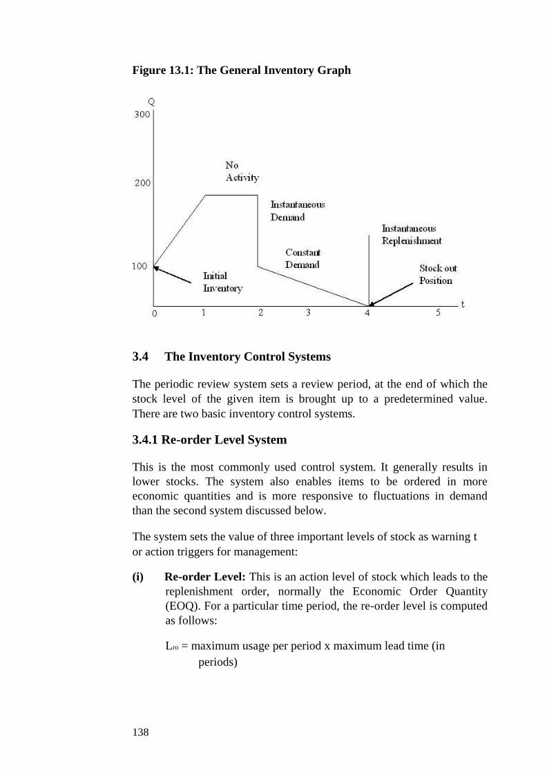
Figure 13.1: The General Inventory Graph

3.4 The Inventory Control Systems

The periodic review system sets a review period, at the end of which the

stock level of the given item is brought up to a predetermined value.

There are two basic inventory control systems.

3.4.1 Re-order Level System

This is the most commonly used control system. It generally results in

lower stocks. The system also enables items to be ordered in more

economic quantities and is more responsive to fluctuations in demand

than the second system discussed below.

The system sets the value of three important levels of stock as warning t

or action triggers for management:

(i) Re-order Level: This is an action level of stock which leads to the

replenishment order, normally the Economic Order Quantity

(EOQ). For a particular time period, the re-order level is computed

as follows:

Lro = maximum usage per period x maximum lead time (in

periods)

138

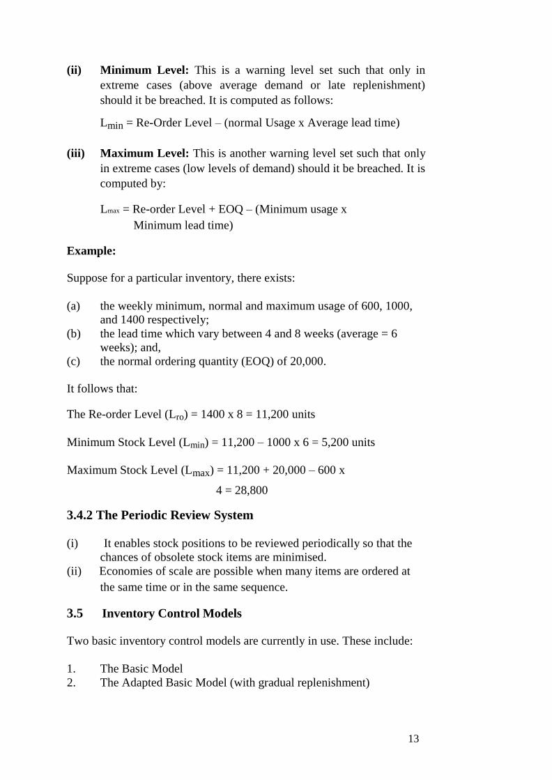
(ii) Minimum Level: This is a warning level set such that only in

extreme cases (above average demand or late replenishment)

should it be breached. It is computed as follows:

Lmin = Re-Order Level – (normal Usage x Average lead time)

(iii) Maximum Level: This is another warning level set such that only

in extreme cases (low levels of demand) should it be breached. It is

computed by:

Lmax = Re-order Level + EOQ – (Minimum usage x

Minimum lead time)

Example:

Suppose for a particular inventory, there exists:

(a) the weekly minimum, normal and maximum usage of 600, 1000,

and 1400 respectively; (b) the lead time which vary between 4 and 8 weeks (average = 6

weeks); and, (c) the normal ordering quantity (EOQ) of 20,000.

It follows that:

The Re-order Level (Lro) = 1400 x 8 = 11,200 units

Minimum Stock Level (Lmin) = 11,200 – 1000 x 6 = 5,200 units

Maximum Stock Level (Lmax) = 11,200 + 20,000 – 600 x

4 = 28,800

3.4.2 The Periodic Review System

(i) It enables stock positions to be reviewed periodically so that the

chances of obsolete stock items are minimised. (ii) Economies of scale are possible when many items are ordered at

the same time or in the same sequence.

3.5 Inventory Control Models

Two basic inventory control models are currently in use. These include:

1. The Basic Model 2. The Adapted Basic Model (with gradual replenishment)

13

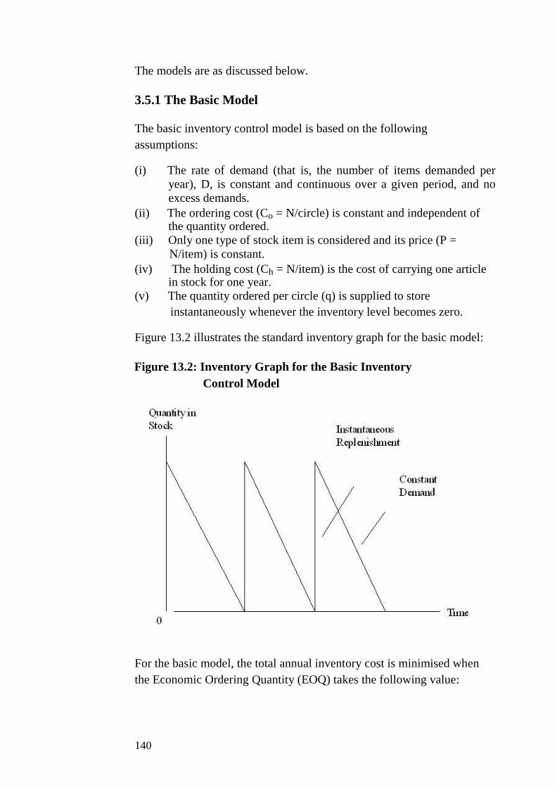
The models are as discussed below.

3.5.1 The Basic Model

The basic inventory control model is based on the following

assumptions:

(i) The rate of demand (that is, the number of items demanded per

year), D, is constant and continuous over a given period, and no

excess demands. (ii) The ordering cost (Co = N/circle) is constant and independent of

the quantity ordered. (iii) Only one type of stock item is considered and its price (P =

N/item) is constant. (iv) The holding cost (Ch = N/item) is the cost of carrying one article

in stock for one year.

(v) The quantity ordered per circle (q) is supplied to store

instantaneously whenever the inventory level becomes zero.

Figure 13.2 illustrates the standard inventory graph for the basic model:

Figure 13.2: Inventory Graph for the Basic Inventory

Control Model

For the basic model, the total annual inventory cost is minimised when

the Economic Ordering Quantity (EOQ) takes the following value:

140

EOQ = 2DCo

Ch Where D = annual demand

Co = Order Cost per circle

Ch = Holding Cost per item

The total annual inventory cost, C, is defined by:

C = Total Ordering Cost + Total Holding Cost

= number of orders per year x order cost + average

inventory level x holding cost per item

C = D/q x Co + q/2 x Ch

Notice from the above equation that as q gets larger:

Annual ordering cost becomes smaller; and annual holding cost

becomes larger.

The basic model also involves the calculation of the following statistics:

(a) Number of orders per year = Yearly Demand

EOQ

(b) Length of Cycle (days) =

Number of Days per year

Number of Orders per year

(c) Average Inventory Level = EOQ

2

Examples:

A commodity has a steady rate of demand of 2,000 units per year.

Placing an order costs N200 and it costs N50 to hold a unit for a year:

(a) Estimate the Economic Order Quantity (EOQ) (b) Find the number of orders placed per year

(c) What is the length of the inventory circle?

Solutions:

Note that from the given information, D = 2,000; Co = 200; and, Ch = 50

141

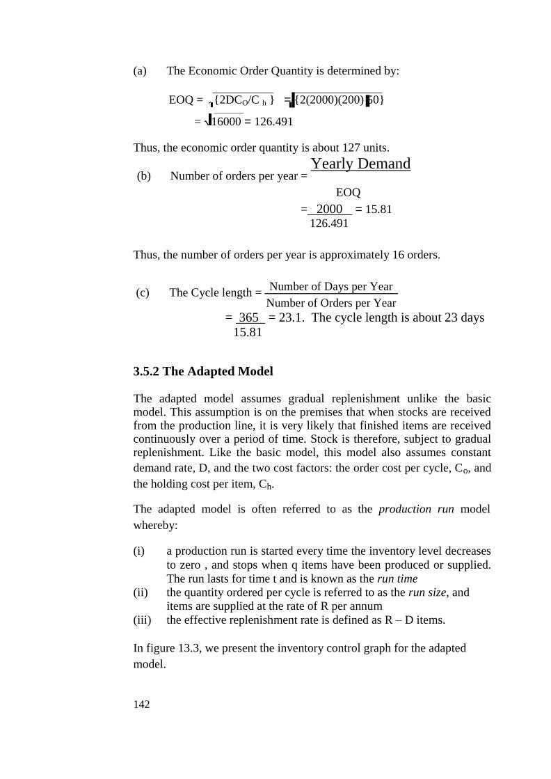
(a) The Economic Order Quantity is determined by:

EOQ = {2DCO/C h } = {2(2000)(200) 50}

= 16000 = 126.491

Thus, the economic order quantity is about 127 units.

(b) Number of orders per year = Yearly Demand

EOQ

= 2000 = 15.81

126.491

Thus, the number of orders per year is approximately 16 orders.

(c) The Cycle length = Number of Days per Year

Number of Orders per Year

= 365 = 23.1. The cycle length is about 23 days

15.81

3.5.2 The Adapted Model

The adapted model assumes gradual replenishment unlike the basic model. This assumption is on the premises that when stocks are received from the production line, it is very likely that finished items are received continuously over a period of time. Stock is therefore, subject to gradual replenishment. Like the basic model, this model also assumes constant

demand rate, D, and the two cost factors: the order cost per cycle, Co, and

the holding cost per item, Ch.

The adapted model is often referred to as the production run model

whereby:

(i) a production run is started every time the inventory level decreases

to zero , and stops when q items have been produced or supplied.

The run lasts for time t and is known as the run time (ii) the quantity ordered per cycle is referred to as the run size, and

items are supplied at the rate of R per annum (iii) the effective replenishment rate is defined as R – D items.

In figure 13.3, we present the inventory control graph for the adapted

model.

142

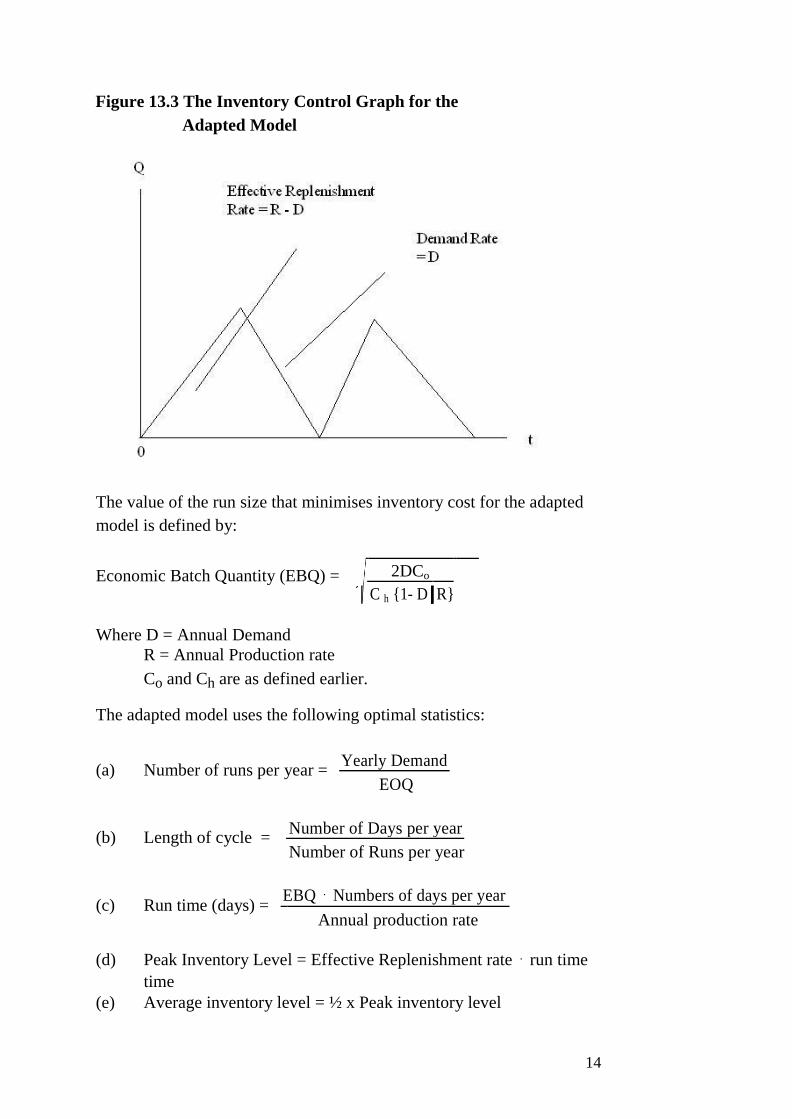
Figure 13.3 The Inventory Control Graph for the

Adapted Model

The value of the run size that minimises inventory cost for the adapted

model is defined by:

Economic Batch Quantity (EBQ) = 2DCo

C h {1- D

R}

Where D = Annual Demand

R = Annual Production rate

Co and Ch are as defined earlier.

The adapted model uses the following optimal statistics:

(a) Number of runs per year = Yearly Demand

EOQ

(b) Length of cycle = Number of Days per year

Number of Runs per year

(c) Run time (days) = EBQ ⋅ Numbers of days per year

Annual production rate

(d) Peak Inventory Level = Effective Replenishment rate ⋅ run time

time

(e) Average inventory level = ½ x Peak inventory level

14

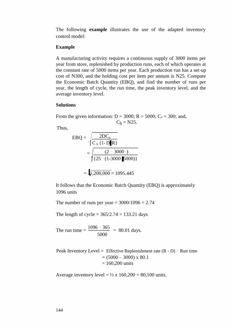
The following example illustrates the use of the adapted inventory

control model:

Example

A manufacturing activity requires a continuous supply of 3000 items per

year from store, replenished by production runs, each of which operates at

the constant rate of 5000 items per year. Each production run has a set-up

cost of N300, and the holding cost per item per annum is N25. Compute

the Economic Batch Quantity (EBQ), and find the number of runs per

year, the length of cycle, the run time, the peak inventory level, and the

average inventory level.

Solutions

From the given information: D = 3000; R = 5000; Co = 300; and,

Ch = N25.

Thus,

EBQ = 2DCo

C h {1- D

R}

= (2 ⋅ 3000⋅)

{25 ⋅(1-3000 5000)}

= 1,200,000 = 1095.445

It follows that the Economic Batch Quantity (EBQ) is approximately

1096 units

The number of runs per year = 3000/1096 = 2.74

The length of cycle = 365/2.74 = 133.21 days

The run time = 1096 ⋅ 365

= 80.01 days. 5000

Peak Inventory Level = Effective Replenishment rate (R - D) ⋅ Run time

= (5000 – 3000) x 80.1 = 160,200 units

Average inventory level = ½ x 160,200 = 80,100 units.

144


1. What is an inventory? Explain some reasons a firm should carry out an inventory

2. What are the differences between EOQ and EBQ?

4.0 CONCLUSION

This unit has looked at inventory control as an essential aspect of

managerial function. This is the life wire of any firm aspiring for growth,

survival, and continuity.

The aim of an inventory control system is to minimise costs and

establish:

(a) the optimum amount of stock to be ordered (b) the period between orders

In a given business organisation, an inventory is defined as the total

stocks of various kinds including: basic raw materials; partly finished

goods and materials; sub-assemblies; office and workshop supplies and

finished goods.

An inventory must be carried by a firm for various reasons.

1. Anticipating normal demand 2. Taking advantage of bulk-purchase discounts

3. Meeting emergency shortages 4. As a natural part of the production process

5. Absorbing wastages and unpredictable fluctuations

5.0 SUMMARY

The discussions in this unit can be summarised as follows:

Just like any other activity in a business setup, the costs associated with

inventories include:

(i) ordering costs; (ii) holding costs; and, (iii) stock out costs

Two basic inventory systems were identified, including:

(i) The Re-order Level system; and, (ii) The Periodic Review system.

14

Two basic inventory control models are currently in use. These include:

1. The Basic Model 2. The Adapted Basic Model


An inventory system follows the adapted basic inventory control model.

The demand rate is constant at 1,600 items per year, the unit price of the

items is N1.80, the holding cost is 10 percent of the unit price per year,

and the set-up cost is N12 per run. If the production rate is 5,000 items

per year, calculate:

(a) the optimum run size (EBQ) (b) the run time

(c) the cycle length (d) the average inventory level


Onwe, O. J. (2007) Statistical Methods for Business and Economic

Decisions: A Practical Approach (Lagos: Samalice Publishers)

146

UNIT 4 DECISION ANALYSIS

CONTENTS

1.0 Introduction

2.0 Objectives

3.0 Main Content

3.1 Certainty and Uncertainty in Decision Analysis

3.2 Analysis of the Decision Problem

3.3 Expected Monetary Value Decisions

3.4 Decision Making Involving Sample Information

4.0 Conclusion

5.0 Summary



1.0 INTRODUCTION

Decision analysis is the modern approach to decision making both in

economics and in business. It can be defined as the logical and

quantitative analysis of all the factors influencing a decision. The

analysis forces decision makers to assume some active roles in the

decision-making process. By so doing, they rely more on rules that are

consistent with their logic and personal behaviour than on the mechanical

use of a set of formulas and tabulated probabilities.

The primary aim of decision analysis is to increase the likelihood of good

outcomes by making good and effective decisions. A good decision must

be consistent with the information and preferences of the decision maker.

It follows that decision analysis provides decision-making framework

based on available information on the business environment, be it sample

information, judgemental information, or a combination of both.

2.0 OBJECTIVES


identify and analyse decision problems

analyse decisions that are made under conditions of certainty and

uncertainties

make expected monetary value decisions

14

3.0 MAIN CONTENT

3.1 Certainty and Uncertainty in Decision Analysis

Most decision-making situations involve the choice of one among

several alternative actions. The alternative actions and their corresponding

payoffs are usually known to the decision-maker in advance. A

prospective investor choosing one investment from several alternative

investment opportunities, a store owner determining how many of a

certain type of commodity to stock, and a company executive making

capital -budgeting decisions are some examples of a business decision

maker selecting from a multitude of alternatives. The decision maker

however, does not know which alternative will be best in each case,

unless he/she also knows with certainty the values of the economic

variables that affect profit. These economic variables are referred to, in

decision analysis, as states of nature as they represent different events

that may occur, over which the decision maker has no control.

The states of nature in decision problems are generally denoted by si (i =

1, 2, 3… k), where k is the number of or different states of nature in a

given business and economic environment. It is assumed here that the

states of nature are mutually exclusive, so that no two states can be in

effect at the same time, and collectively exhaustive, so that all possible

states are included within the decision analysis.

The alternatives available to the decision maker are denoted by

ai (i = 1, 2, 3, …, n), where n is the number of available alternatives. It is

also generally assumed that the alternatives constitute a mutually

exclusive, collectively exhaustive set.

When the state of nature, si, whether known or unknown, has no

influence on the outcomes of given alternatives, we say that the decision

maker is operating under certainty. Otherwise, he/she is operating under

uncertainty.

Decision making under certainty appears to be simpler than that under

uncertainty. Under certainty, the decision maker simply appraises the

outcome of each alternative and selects the one that best meets his/her

objective. If the number of alternatives is very high however, even in the

absence of uncertainty, the best alternative may be difficult to identify.

Consider, for example, the problem of a delivery agent who must make

100 deliveries to different residences scattered over Lagos metropolis.

There may literally be thousands of different alternative routes the agent

could choose. However, if the agent had only 3 stops to make, he/she

could easily find the least-cost route.

148

Decision making under uncertainty is always complicated. It is the

probability theory and mathematical expectations that offer tools for

establishing logical procedures for selecting the best decision alternatives.

Though statistics provides the structure for reaching the decision, the

decision maker has to inject his/her intuition and knowledge of the

problem into the decision- making framework to arrive at the decision

that is both theoretically justifiable and intuitively appealing. A good

theoretical framework and commonsense approach are both essential

ingredients for decision making under uncertainty.

To understand these concepts, consider an investor wishing to invest

N100, 000 in one of three possible investment alternatives, A, B, and C.

Investment A is a Savings Plan with returns of 6 percent annual interest.

Investment B is a government bond with 4.5 percent annual interest.

Investments A and B involve no risks. Investment C consists of shares of

mutual fund with a wide diversity of available holdings from the

securities market. The annual return from an investment in C depends on

the uncertain behaviour of the mutual fund under varying economic

conditions.

The investors available actions (ai; I = 1, 2, 3, 4) are as follows

a1: do not invest

a2: select investment A the 6% bank savings plan.

a3: select investment B, the 4.5 % government bond.

a4: select investment C, the uncertain mutual fund

Observe that actions a1 to a3 do not involve uncertainty as the outcomes

associated with them do not depend on uncertain market conditions. Observe also that action a 2 dominates actions a1 and a3. In addition,

action a1 is clearly inferior to the risk-free positive growth investment

alternatives a2 and a3 as it provides for no growth of the principal amount.

Action a4 is associated with an uncertain outcome that, depending on the state of the economy, may produce either a negative return or a positive return. Thus there exists no apparent dominance relationship between

action a4 and action a2, the best among the actions involving no

uncertainty.

Suppose the investor believes that if the market is down in the next year,

an investment in the mutual fund would lose 10 percent returns; if the

market stays the same, the investment would stay the same; and if the

market is up, the investment would gain 20 percent returns. The investor

has thus defined the states of nature for his/her investment decision-

making problem as follows:

14

s1: the market is down.

s2: the market remains unchanged.

s3: the market is up.

A study of the market combined with economic expectations for the

coming year may lead the investor to attach subjective probabilities of

0.25, 0.25, and 0.50, respectively, the states of nature, s1, s2, and s3. The

major question is then, how can the investor use the foregoing

information regarding investments A, B, and C, and the expected market

behaviour serves as an aid in selecting the investment that best satisfies

his/her objectives? This question will be considered in the sections that

follow.

3.2 Analysis of the Decision Problem

In problems involving choices from many alternatives, one must identify

all the actions that may be taken and all the states of nature which

occurrence may influence decisions. The action to take none of the listed

alternatives whose outcome is known with certainty may also be included

in the list of actions. Associated with each action is a list of payoffs. If an

action does not involve risk, the payoff will be the same no matter which

state of nature occurs.

The payoffs associated with each possible outcome in a decision problem

should be listed in a payoff table, defined as a listing, in tabular form, of

the value payoffs associated with all possible actions under every state of

nature in a decision problem.

The payoff table is usually displayed in grid form, with the states of nature indicated in the columns and the actions in the rows. If the actions

are labeled a1, a 2… an, and the states of nature labeled s1, s2, …,

sk, a payoff table for a decision problem appears as in table 14.1 below.

Note that a payoff is entered in each of the nk cells of the payoff table,

one for the payoff associated with each action under every possible state

of nature.

Table 14.1: The Payoff Table

State of Nature

ACTION s1 s2 s3 … sk

a1

a2

a3 .

.

.

an

150

Example

The managing director of a large manufacturing company is considering

three potential locations as sites at which to build a subsidiary plant. To

decide which location to select for the subsidiary plant, the managing

director will determine the degree to which each location satisfies the

company’s objectives of minimising transportation costs, minimising the

effect of local taxation, and having access to an ample pool of available

semi-skilled workers. Construct a payoff table and payoff measures that

effectively rank each potential location according to the degree to which

each satisfies the company’s objectives.

Solution

Let the three potential locations be sites A, B, and C. To determine a

payoff measure to associate with each of the company’s objectives under

each alternative, the managing director subjectively assigns a rating on a 0

to 10 scale to measure the degree to which each location

satisfies the company’s objectives. For each objective, a 0 rating indicates

complete dissatisfaction, while a 10 rating indicates complete

dissatisfaction. The results are presented in table 14.2 below:

Table 14.2: Ratings for three alternative plant sites for

a Manufacturing Company

ALTERNATIVE

COMPANY OBJECTIVE Site A Site B Site C

Transportation Costs 6 4 10

Taxation Costs 6 9 5

Workforce Pool 7 6 4

To combine the components of payoff, the managing director asks

himself, what are the relative measures of importance of the three

company objectives I have considered as components of payoff? Suppose

the managing director decides that minimising transportation costs is most

important and twice as important as either the minimisation of local

taxation or the size of workforce available. He/she thus assigns a weight

of 2 to the transportation costs and weights of 1 each to taxation costs and

workforce. This will give rise to the following payoff measures:

Payoff (Site A) = 6(2) + 6(1) + 7(1) = 25

Payoff (Site B) = 4(2) + 9(1) + 6(1) = 23

Payoff (Site C) = 10(2) + 5(1) + 4(1) = 29

15

3.3 Expected Monetary Value Decisions

A decision-making procedure, which employs both the payoff table and

prior probabilities associated with the states of nature to arrive at a

decision, is referred to as the Expected Monetary Value decision

procedure. Note that by prior probability, we mean probabilities

representing the chances of occurrence of the identifiable states of nature

in a decision problem prior to gathering any sample information. The

expected monetary value decision refers to the selection of available

action based on either the expected opportunity loss or the expected profit

of the action.

Decision makers are generally interested in the optimal monetary value

decisions. The optimal expected monetary value decision involves the

selection of the action associated with the minimum expected opportunity

loss or the action associated with the maximum expected profit,

depending on the objective of the decision maker.

The concept of expected monetary value applies mathematical

expectation, where opportunity loss or profit is the random variable and

the prior probabilities represent the probability distribution associated

with the random variable.

The expected opportunity loss is computed by:

E (Li) = ∑all j LijP(sj), (i = 1, 2, …, n)

Where Lij is the opportunity loss for selecting action ai given that the state

of nature, sj, occurs and P (sj) is the prior probability assigned to the state

of nature, sj.

The expected profit for each action is computed in a similar way:

E (πi) = ∑all j πijP(sj)

Where πij represents profits for selecting action

ai Example

By recording the daily demand for a perishable commodity over a period

of time, a retailer was able to construct the following probability

distribution for the daily demand levels:

152

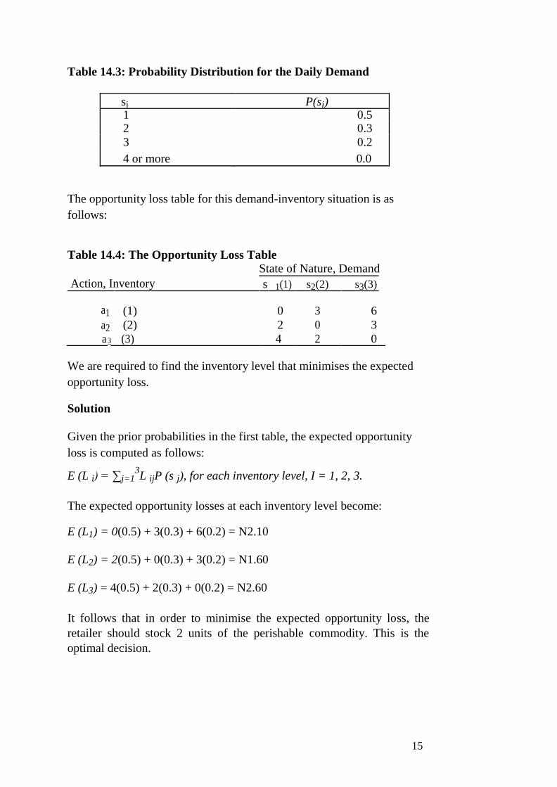
Table 14.3: Probability Distribution for the Daily Demand

sj P(sj) 1 0.5 2 0.3

3 0.2

4 or more 0.0

The opportunity loss table for this demand-inventory situation is as

follows:

Table 14.4: The Opportunity Loss Table

Action, Inventory

State of Nature, Demand

s 1(1) s2(2) s3(3)

a1 (1) 0 3 6

a2 (2) 2 0 3

a 3 (3) 4 2 0

We are required to find the inventory level that minimises the expected

opportunity loss.

Solution

Given the prior probabilities in the first table, the expected opportunity

loss is computed as follows:

E (L i) = ∑j=13L ijP (s j), for each inventory level, I = 1, 2, 3.

The expected opportunity losses at each inventory level become:

E (L1) = 0(0.5) + 3(0.3) + 6(0.2) = N2.10

E (L2) = 2(0.5) + 0(0.3) + 3(0.2) = N1.60

E (L3) = 4(0.5) + 2(0.3) + 0(0.2) = N2.60

It follows that in order to minimise the expected opportunity loss, the

retailer should stock 2 units of the perishable commodity. This is the

optimal decision.

15

3.4 Decision Making Involving Sample Information

Prior probabilities are acquired either by subjective selection or by

computation from historical data. No current information describing the

probability of occurrence of the states of nature was assumed to be

available.

In many cases, observational information or other evidences are available

to the decision maker either for purchase or at the cost of

experimentation. For example, a retailer whose business depends on the

weather may consult a meteorologist before making decisions, or an

investor may hire a market consultant before investing. Market surveys

carried out before the release of a new product represent another area in

which the decision maker may seek additional information. In each of

these examples, the decision maker attempts to acquire information

relative to the occurrence of the states of nature from a source other than

that from which the prior probabilities were computed.

When such information is available, Baye’s Law can be employed to

revise the prior probabilities to reflect the new information. These revised

probabilities are referred to as posterior probabilities.

By definition, the posterior probability represented symbolically by P

(sk/x) is the probability of occurrence of the state of nature sk, given the

sample information, x. This probability is computed by:

P(s k/x) = P(x/sk )P(sk )

all i P(x/si )P(si )

The probabilities,

the observational

probabilities P (si)

P(x/si) are the conditional probabilities of observing

information, x, under the states of nature, si, and the are

the prior probabilities.

The expected monetary value decisions are formulated in the same way as

before, except that the posterior probabilities are used instead of prior

probabilities. If the objective is to minimise the expected opportunity loss,

the quantity is computed for each action . The expected opportunity loss

in this case is computed by:

E (Li) = ∑all I LijP(si/x) I = 1, 2, 3,…,n

Example

It is known that an assembly machine operates at a 5 percent or 10

percent defective rate. When running at a 10 percent defective rate, the

machine is said to be out of control. It is then shut down and readjusted.

154

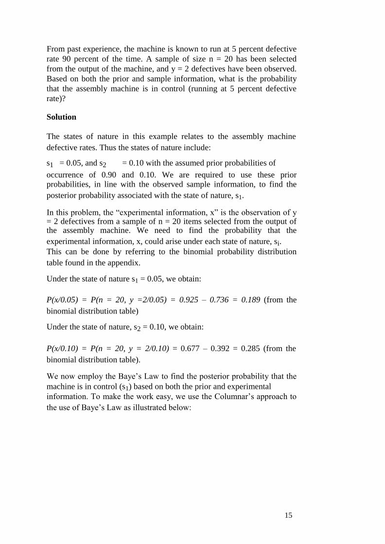
From past experience, the machine is known to run at 5 percent defective

rate 90 percent of the time. A sample of size n = 20 has been selected

from the output of the machine, and y = 2 defectives have been observed.

Based on both the prior and sample information, what is the probability

that the assembly machine is in control (running at 5 percent defective

rate)?

Solution

The states of nature in this example relates to the assembly machine

defective rates. Thus the states of nature include:

s1 = 0.05, and s2 = 0.10 with the assumed prior probabilities of

occurrence of 0.90 and 0.10. We are required to use these prior probabilities, in line with the observed sample information, to find the

posterior probability associated with the state of nature, s1.

In this problem, the “experimental information, x” is the observation of y = 2 defectives from a sample of n = 20 items selected from the output of the assembly machine. We need to find the probability that the

experimental information, x, could arise under each state of nature, si.

This can be done by referring to the binomial probability distribution

table found in the appendix.

Under the state of nature s1 = 0.05, we obtain:

P(x/0.05) = P(n = 20, y =2/0.05) = 0.925 – 0.736 = 0.189 (from the

binomial distribution table)

Under the state of nature, s2 = 0.10, we obtain:

P(x/0.10) = P(n = 20, y = 2/0.10) = 0.677 – 0.392 = 0.285 (from the

binomial distribution table).

We now employ the Baye’s Law to find the posterior probability that the

machine is in control (s1) based on both the prior and experimental

information. To make the work easy, we use the Columnar’s approach to

the use of Baye’s Law as illustrated below:

15

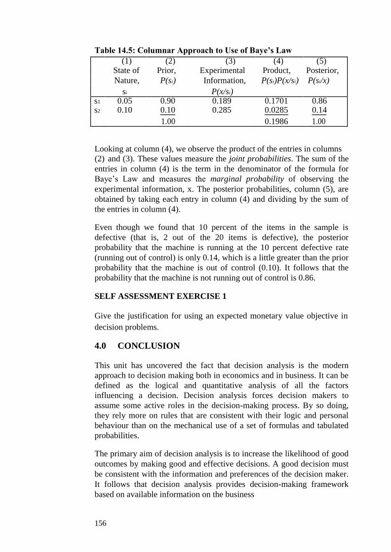
Table 14.5: Columnar Approach to Use of Baye’s Law

(1) (2) (3) (4) (5)

State of Prior, Experimental Product, Posterior,

Nature, P(si) Information, P(si)P(x/si) P(si/x)

si P(x/si)

s1 0.05 0.90 0.189 0.1701 0.86 s2 0.10 0.10 0.285 0.0285 0.14

1.00 0.1986 1.00

Looking at column (4), we observe the product of the entries in columns

(2) and (3). These values measure the joint probabilities. The sum of the

entries in column (4) is the term in the denominator of the formula for

Baye’s Law and measures the marginal probability of observing the

experimental information, x. The posterior probabilities, column (5), are

obtained by taking each entry in column (4) and dividing by the sum of

the entries in column (4).

Even though we found that 10 percent of the items in the sample is

defective (that is, 2 out of the 20 items is defective), the posterior

probability that the machine is running at the 10 percent defective rate

(running out of control) is only 0.14, which is a little greater than the prior

probability that the machine is out of control (0.10). It follows that the

probability that the machine is not running out of control is 0.86.


Give the justification for using an expected monetary value objective in

decision problems.

4.0 CONCLUSION

This unit has uncovered the fact that decision analysis is the modern

approach to decision making both in economics and in business. It can be

defined as the logical and quantitative analysis of all the factors

influencing a decision. Decision analysis forces decision makers to

assume some active roles in the decision-making process. By so doing,

they rely more on rules that are consistent with their logic and personal

behaviour than on the mechanical use of a set of formulas and tabulated

probabilities.

The primary aim of decision analysis is to increase the likelihood of good

outcomes by making good and effective decisions. A good decision must

be consistent with the information and preferences of the decision maker.

It follows that decision analysis provides decision-making framework

based on available information on the business

156

environment, be it sample information, judgemental information, or a

combination of both.

5.0 SUMMARY

The unit considered the following important elements of decision

analysis:

1. Decision Problems and Analysis

In problems involving choices from many alternatives, one must identify

all the actions that may be taken and all the states of nature whose

occurrence may influence decisions. The action to take none of the listed

alternatives whose outcome is known with certainty may also be included

in the list of actions. Associated with each action is a list of payoffs. If an

action does not involve risk, the payoff will be the same no matter which

state of nature occurs.

2. Expected Monetary Value Decisions

A decision-making procedure, which employs both the payoff table and

prior probabilities associated with the states of nature to arrive at a

decision, is referred to as the Expected Monetary Value decision

procedure. Note that by prior probability we mean probabilities

representing the chances of occurrence of the identifiable states of nature

in a decision problem prior to gathering any sample information. The

expected monetary value decision refers to the selection of available

action based on either the expected opportunity loss or the expected profit

of the action.

3. Decision Making Involving Sample Information

In many decisions, observational information or other evidence are

available to the decision maker either for purchase or at the cost of

experimentation. For example, a retailer whose business depends on the

weather may consult a meteorologist before making decisions, or an

investor may hire a market consultant before investing. Market surveys

carried out before the release of a new product represent another area in

which the decision maker may seek additional information. In each of

these examples, the decision maker attempts to acquire information

relative to the occurrence of the states of nature from a source other than

that from which the prior probabilities were computed.

When such information is available, Baye’s Law can be employed to

revise the prior probabilities to reflect the new information. We refer to

such probabilities as posterior probabilities.

15


A special commission appointed by the governor of Enugu state is currently studying the issue of site location for a nuclear power-

generating plant. The alternatives being currently considered are (a1) to

locate the plant at the mouth of Ever-Valley River, (a2) to locate the plant

inland, and (a3) not to build the plant at all. Because of the heat generated

in cooling operations, a1 may prove damaging to a nearby fishing industry vital to the economy of Enugu state. However, there may

be insufficient water flow available at site a2 for adequate cooling.

If alternative a3 is chosen, sufficient energy resources may not be

available to meet future needs.

(a) If you were the economic adviser to the commission, what would

you recommend to be used as a measure of payoff for evaluating

the three alternatives?

(b) Suppose the commission has decided that the important

attributes of value in the decision model are

(i) the ability of each alternative to meet future commercial

power needs,

(ii) the ability of each alternative to meet future residential

power needs,

(iii) the effects on the state’s fishing industry, and

(iv) other environmental effects. What recommendation would

you give to the commission regarding the incorporation of

these four attributes into a model to derive some reasonable

measure of payoff associated with each alternative?



edition

(Great Britain: Ashford Colour Press).

158

UNIT 5 NETWORK PLANNING AND ANALYSIS

CONTENTS

1.0 Introduction

2.0 Objectives

3.0 Main Content

3.1 Activities and Events

3.2 Summary of Network Planning Processes 3.3 Critical Paths

3.3.1 Earliest and Latest Event Times Approach to

Critical Path

3.3.2 Tabular Presentation of a Network

4.0 Conclusion

5.0 Summary



1.0 INTRODUCTION

This unit recognises the managerial importance of networking in

production, distribution, and related business activities. Network

planning is basically the task of breaking down a given business project

into its constituent activities and deciding on their time relationships. It

involves listing the activities needed to complete a project, as well as

defining the time for the completion, organising the order of completion

of the activities, and drawing the associated network. This task is very

valuable as it can help management in the establishment of objectives and

in pinpointing the courses of action to follow. The resulting network chart

forms a policy statement.

Network analysis covers the way large projects are planned. Such

projects include a major construction work, research and development

projects, the computerisation of business activities, and the like.

2.0 OBJECTIVES


define activities and events

construct activity networks

construct precedence

tables

state the network planning

processes

explain the critical path analysis.

15

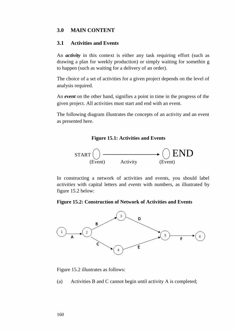
3.0 MAIN CONTENT

3.1 Activities and Events

An activity in this context is either any task requiring effort (such as

drawing a plan for weekly production) or simply waiting for somethin g

to happen (such as waiting for a delivery of an order).

The choice of a set of activities for a given project depends on the level of

analysis required.

An event on the other hand, signifies a point in time in the progress of the

given project. All activities must start and end with an event.

The following diagram illustrates the concepts of an activity and an event

as presented here.

Figure 15.1: Activities and Events

START

END

(Event) Activity (Event)

In constructing a network of activities and events, you should label

activities with capital letters and events with numbers, as illustrated by

figure 15.2 below:

Figure 15.2: Construction of Network of Activities and Events

Figure 15.2 illustrates as follows:

(a) Activities B and C cannot begin until activity A is completed;

160

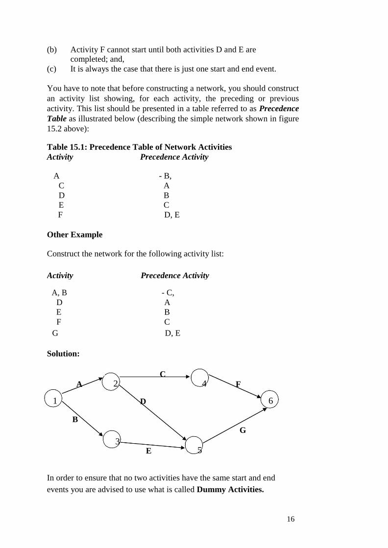
(b) Activity F cannot start until both activities D and E are completed; and,

(c) It is always the case that there is just one start and end event.

You have to note that before constructing a network, you should construct

an activity list showing, for each activity, the preceding or previous

activity. This list should be presented in a table referred to as Precedence

Table as illustrated below (describing the simple network shown in figure

15.2 above):

Table 15.1: Precedence Table of Network Activities

Activity Precedence Activity

A - B,

C A

D B

E C

F D, E

Other Example

Construct the network for the following activity list:

Activity Precedence Activity

A, B - C,

D A

E B

F C

G D, E

Solution:

A 2 C

4 F

1 D 6

B

G

3

E

5

In order to ensure that no two activities have the same start and end

events you are advised to use what is called Dummy Activities.

16

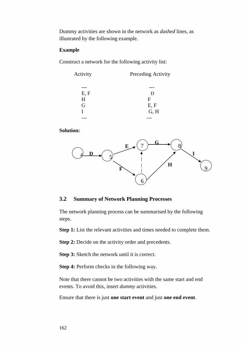
Dummy activities are shown in the network as dashed lines, as

illustrated by the following example.

Example

Construct a network for the following activity list:

Activity Preceding Activity

--- ---

E, F D

H F G E, F

I G, H

--- ---

Solution:

E 7

G 8

D

4 5 I

H

F

9

6

3.2 Summary of Network Planning Processes

The network planning process can be summarised by the following

steps.

Step 1: List the relevant activities and times needed to complete them.

Step 2: Decide on the activity order and precedents.

Step 3: Sketch the network until it is correct.

Step 4: Perform checks in the following way.

Note that there cannot be two activities with the same start and end

events. To avoid this, insert dummy activities.

Ensure that there is just one start event and just one end event.

162

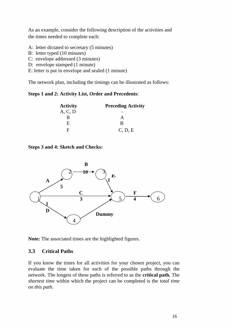
As an example, consider the following description of the activities and

the times needed to complete each:

A: letter dictated to secretary (5 minutes) B: letter typed (10 minutes) C: envelope addressed (3 minutes)

D: envelope stamped (1 minute) E: letter is put in envelope and sealed (1 minute)

The network plan, including the timings can be illustrated as follows:

Steps 1 and 2: Activity List, Order and Precedents:

Activity Preceding Activity

A, C, D -

B A

E B

F C, D, E

Steps 3 and 4: Sketch and Checks:

B

2 10 3

A 1 E

5

C

F

1 5 6 3 4 1

D Dummy

4

Note: The associated times are the highlighted figures.

3.3 Critical Paths

If you know the times for all activities for your chosen project, you can

evaluate the time taken for each of the possible paths through the

network. The longest of these paths is referred to as the critical path. The

shortest time within which the project can be completed is the total time

on this path.

16

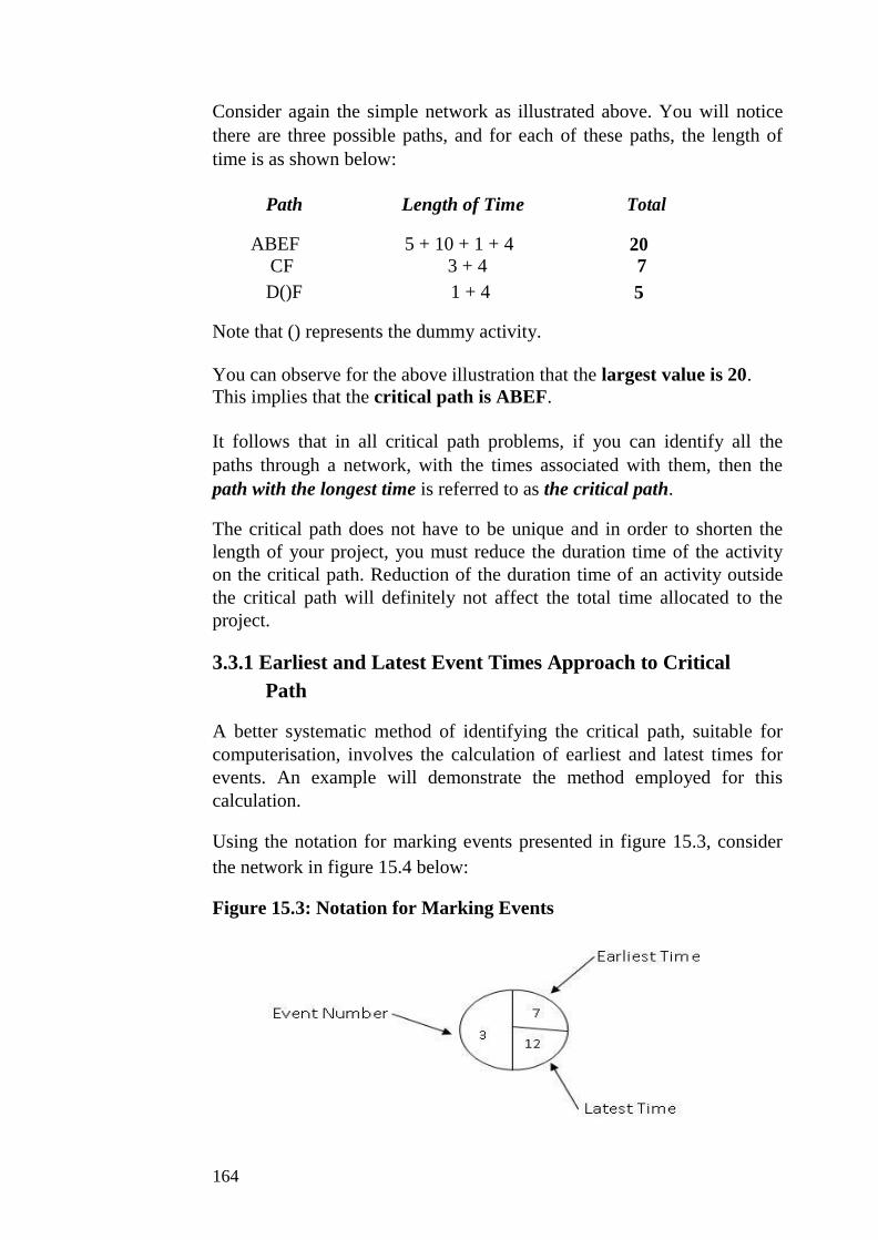
Consider again the simple network as illustrated above. You will notice

there are three possible paths, and for each of these paths, the length of

time is as shown below:

Path Length of Time Total

ABEF 5 + 10 + 1 + 4 20

CF 3 + 4 7

D()F 1 + 4 5

Note that () represents the dummy activity.

You can observe for the above illustration that the largest value is 20.

This implies that the critical path is ABEF.

It follows that in all critical path problems, if you can identify all the

paths through a network, with the times associated with them, then the

path with the longest time is referred to as the critical path.

The critical path does not have to be unique and in order to shorten the

length of your project, you must reduce the duration time of the activity

on the critical path. Reduction of the duration time of an activity outside

the critical path will definitely not affect the total time allocated to the

project.

3.3.1 Earliest and Latest Event Times Approach to Critical

Path

A better systematic method of identifying the critical path, suitable for

computerisation, involves the calculation of earliest and latest times for

events. An example will demonstrate the method employed for this

calculation.

Using the notation for marking events presented in figure 15.3, consider

the network in figure 15.4 below:

Figure 15.3: Notation for Marking Events

164

Figure 15.4: Calculation of earliest and latest times for events

Figure 15.4.1: Original Network

2

A

6 D 2

1

B

4 4 E

3 3

To enter the earliest time, you work from left to right in the original

network and enter ‘0’ in event 1 early.

The basic technique is to simply go to each event in turn, adding the

activity time to the previous event early time. For example, event 2 early

= E (2) = E (1) + A = 0 + 2 = 2. You need to note that in this process, you

should follow the arrow head, and if there is more than one arrow head

leading to an event, you should take the largest of the possible early

times.

Completing the process, E (3) = E (1) + B = 0 + 4 =

4; E (4) = E (2) + D = 2 + 6 = 8

The earliest time entered is presented below:

Figure 15.4.2: The earliest times entered

16

You can now work backwards starting from the final event, event E (4),

and fill in all the latest event times.

Start with the event time for the last event, E (4) = 8.

You can now calculate the event late time = L (event) for each event by

subtracting the activity time from L(previous). Thus, for the event before

event 4, E (4) which is event 3 or E (3), the event late time will be: L (3)

= L (4) – E = 8 – 3 = 5. For events with two possibilities (or two arrow

heads, the rule will be the reverse of the earlier discussed event choice

circle; if there are more than one tail or arrow head leading from the

event, you would have to take the smallest difference. This happens to be

the case for event 2.

For the event 2, you can observe the choice of 8 – 6 = 2 or 5 – 1 = 4. It

follows that by this rule, L (2) = 2. These calculations are presented in

figure 13.4.3 below:

Figure 15.4.3: Earliest and Latest Times Entered

2

2

2

A D

6 2

1 0 8

0

4

8

B E

4 4 3

3 5

To summarise these discussions, note the followings:

Earliest (E) Calculation: E(event) = E(previous event) + Activity Time

If there are more than one arrow heads leading to an event, choose the

largest event time.

166

Latest (L) Calculation: L (event) = L (next event) – Activity

Time If there are ‘tail’ alternatives, choose the smallest event time.

3.4.2 Tabular Presentation of a Network

Activity networks can be presented in a tabular form, showing activity

name, duration, and earliest and latest start and finish times. In the

following example, you will learn how the tabular presentation of

networks can be done. As a guide, note first the following relationships:

1. Earliest activity start time = Earliest start of beginning event 2. Earliest activity finish time = Earliest start of beginning event

+ activity duration 3. Latest activity start time = Latest start of ending event – activity

duration 4. Latest activity finish time = Latest start of ending event

The Example

You are required to put in a tabular form the following network

Solution

Activity Duration Start Finish

E L E L

1 - 2 4 0 0 4 4

1 - 3 2 0 7 2 9

2 - 4 3 4 13 7 16

2 - 5 8 4 4 12 12

3 - 5 3 2 9 5 12

4 - 6 2 7 16 9 18

5 - 6 6 12 12 18 18

16


1. Define activities and event as used in network analysis 2. What is a precedence table?

2. Why are dummy activities necessary? 3. What do we mean by a critical path through a network?

4.0 CONCLUSION

This unit has discussed at length the basic principles of activity

networking. You have been exposed to the following very important

issues.

1) Activity and events; 2) Construction of network of activities and events;

3) Meaning and construction of precedence table; 4) Network planning processes; and,

5) The critical path analysis

5.0 SUMMARY

The importance of networking in production cannot be over emphasised.

As pointed out in this unit, network planning appears to be basically the

task of breaking down a given business project into its constituent

activities and deciding on their time relationships. It involves listing the

activities needed to complete a project, as well as defining the time for the

completion, organising the order of completion of the activities, and

drawing the associated network. This task is very valuable as it can help

management in the establishment of objectives and in pinpointing the

courses of action to follow. The resulting network chart forms a policy

statement.

Network analysis in itself covers the way large projects are planned. Such

projects include a major construction work, research and development

projects, the computerisation of business activities, and the like.

Other important management issues discussed have to do with critical

path analysis. We noted that, if you know the times for all activities for

your chosen project, you can evaluate the time taken for each of the

possible paths through the network. The longest of these paths is referred

to as the critical path. The shortest time within which the project can be

completed is the total time on this path.

168


The following activities describe the project of ‘changing a flat tyre’.

The bracketed figures are timing in minutes.

A = take jack and tools from the boot (1)

B = remove wheel cover (0.5)

C = loosen wheel nuts (1.5)

D = place jack under car ((0.5)

E = jack up the car (0.5)

F = get spare tyre from the boot (0.40)

G = remove wheel nuts and the wheel (0.5)

H = place spare tyre onto the studs (0.25)

I = guide nuts onto studs (0.15)

J = lower car and remove jack (0.25) K = replace jack in boot (0.15)

L = tighten nuts on studs (0.25)

M = put old wheel and tools back to the boot (1)

N = replace wheel cover (0.5)

(a) Draw up the relevant precedence table (b) Draw up the network (c) Draw up a table showing duration, earliest and latest activity

times.



edition

(Great Britain: Ashford Colour Press)

16

MODULE 4

Unit 1 Arithmetic and Geometric Progression

Unit 2 Interest Rate and Depreciation

Unit 3 Present Values and Investment Analysis

UNIT 1 ARITHMETIC AND GEOMETRIC

PROGRESSION

1.0 Introduction

2.0 Objectives

3.0 Main Content

3.1 Progressions

3.2 Arithmetic Progressions (AP)

3.3 Geometric Progression (GP)

4.0 Conclusion

5.0 Summary



1.0 INTRODUCTION

As a preliminary, this unit begins with discussions on sequences of

numbers referred to as arithmetic and geometric progressions. The form

of each of these, including the formulae for calculating the totals are also

discussed. The important practical business applications of progression

will be presented for your future adaptation to investment decisions.

2.0 OBJECTIVES


interpret the concepts of arithmetic and geometric progressions

explain the computational formulae for arithmetic and

geometric progression

apply the concepts of progressions in daily business and

investment decisions.

170

3.0 MAIN CONTENT

3.1 Progressions

Mathematical progressions that are often used in business and economics

are those of Arithmetic and Geometric progressions. These feature mostly

in mathematics of finance, where they are used in calculating interest

earnings on investments. Taking these progressions one at a time, discuss

as follows.

3.2 Arithmetic Progressions (AP)

An arithmetic progression refers to a sequence of numbers, called terms,

in which any number after the first can be obtained from the immediate

past number by adding a constant number, called the common

difference, d.

The sequence of numbers: 1, 5, 9, 13, 17, 21, for example is an arithmetic

progression, since the common difference between one term and the next

is 4 (5 – 1 = 4; 9 – 5 = 4; 13 – 9 = 4, etc.). The constant difference, 4, is

the common difference, d.

The first term of an arithmetic progression can be denoted by a. This

implies that an arithmetic progression takes the general form:

a, a + d, a + 2d, a + 3d, a + 4d …

The value of a particular term, the n-th term, and sum of the terms in an

arithmetic progression can be ascertained using the following formulae:

1. n-th term = an = a + (n – 1) d,

Where a refers to the first-term; n refers to the number of terms

in the sequence; and d refers to the common difference.

2. Sum of the n terms in the sequence = Sn = n/2 [2a + (n – 1) d]

Examples

Consider the progression: 10, 15, 20, 25 … This is an arithmetic

progression (AP) as each term is obtained by adding 5 to the previous

term. The first term in this progression is 10 and the common difference,

d = 5.

To find the value of the 6th

term, a6, and the sum of the first 8 terms of

this progression, you will do the following:

17

First, identify the progression (AP), with first term, a = 10 and the

common difference, d = 5. From the formula,

an = a + (n – 1)d, you get:

6th

- term = a6 = 10 + (6 – 1) (5), since n = 6.

a6 = 10 + 25 = 35.

It follows that the 6th

term of this progression has the value of 35.

You will obtain the sum of the first 8 terms of this progression using the

stated formula for the sum of n terms (that is, 8 terms in this case):

Sn = S8 = 8/2 [2a + (n – 1) d]

= 4[2(10) + (8 – 1) (5)]

= 4[20 + 35]

= 4(55)

= 220.

This means that the sum of the first 8 terms of the progression in question

is 220.

3.3 Geometric Progression (GP)

A Geometric Progression (GP) defines a sequence of numbers, referred to

as terms, in which any term after the first can be obtained from its

immediate past term or predecessor by multiplying this past term by a

constant term, called the common ratio (r). Like the arithmetic

progression, the first term of the geometric progression is denoted by the

letter a.

For instance, the sequence of the numbers: 5, 15, 45, 135 … is a

geometric progression since each term is being multiplied by the same

constant term (3 in this case) to obtain the next term in the sequence.

Notice that you can obtain this constant term (that is 3) by dividing the

new term by its immediate past term or predecessor: 15/5 = 3; 45/15 = 3;

and 135/45 = 3. This constant term is the common ratio denoted by r.

The general form of Geometric Progression can be presented as follows:

GP = a, ar, ar2, ar

3, ar

4…

172

In our example above, a = 5 and r =3, given the geometric progression

as:

5, 5(3), 5(3)2, 5(3)

3

Or, 5, 15, 45, 135

Formulae for a Geometric Progression

If the first term of a geometric progression is given as the letter a and

the common ratio given as r, then:

1. the nth –term can be determined by: an = arn-1

2. Sum of the first n terms can be obtained by:

Sn = a(rn - 1) = a(1 - r

n)

r - 1 1 - r

If the absolute value of r, /r/ < 1, the sum to infinity is:

S∞ = a/ (1 – r)

Examples

1. Can you find the 7th

term and the sum of the first 10 terms of the

geometric progression: 5, 15, 45, 135 …

Solution

First, you should identify this series a geometric progression with the first

term, a = 5, and common ratio, r = 3. Then using the formula for the nth-

term of a geometric progression, you get:

an = arn-1

, where n = 7

a7 = 5(3)7-1

= 5(3)6 = 3,645

Using the formula for the sum of a geometric progression, you get:

a(r n - 1)

Sn = r - 1

17

Sum of the first 10 terms = S10 = 5[(3)

10 1]

3 1

= 5[59049 1]

2

= 295,240

2 = 147,620

2. Find the sum to infinity of the geometric

progression: 16, 4, 1, 0.25 … etc

Solution

Notice that in this progression, a = 16 and r = 4/16 = 1/4 =

… = 0.25 < 1

Recall that the sum to infinity is formulated as:

S∞ = a/ (1 – r), since r < 1 in this example.

Thus S∞ = 16/ (1 – 0.25) = 16/ 0.75 = 21.33.


1. Discuss briefly the basic difference between Arithmetic and

Geometric Progressions

2. If the first term and common ratio of a geometric progression are

denoted by a and r, respectively, what is the expression used in

calculating the sum of the first n terms?

4.0 CONCLUSION

This unit has presented the basic principles of progressions, with special

emphasis on arithmetic and geometric progressions. The major

conclusions you can draw from the discussions are that:

1. the most important applications of progressions in business

decisions are in the areas of determination of the numeric values of

any term and sum of a given mathematical series.

2. the basic difference between an arithmetic progression and a

geometric progression is in their constant factors: the common

174

difference for an arithmetic progression; and, the common ratio

in a geometric progression.

3. identification of the first term and the common factors will enable

you know whether a given numeric series is an arithmetic series or

a geometric series.

5.0 SUMMARY

The major points you may have learned from this unit can be

summarised as follows:

1. An arithmetic progression is of the form: a, a + d, a + 2d, A + 3d.

where d represents the common difference, and a represents the

first term. 2. The n-th of an arithmetic progression (AP) is given

by: an = a + (n – 1)d 3. The sum of the first n terms of an AP is given

by: Sn = n/2[2a + (n – 1)d]

4. A geometric progression is of the form: a, ar, ar2, ar

3…

where a is the first term and r represents the common ratio. 5. The n-th term of a geometric progression is obtained

by: an = arn - 1

6. The sum of the first n-terms of a geometric progression is obtained

by:

Sn = a(rn - 1) = a(1 - r

n)

r - 1 1 - r

7. Sum of a geometric progression to infinity can be obtained

by: S∞ = a/ (1 – r)


(1) Find the sum of the first 15 terms of the

progression: 48, 40, 32, 24 … (2) Find the 6

th term and the sum of the first 8 terms of the

progression: 1, 3, 9, 27 … (3) Find the sum to infinity of the progression:

14, 14(0.8), 14(0.8)2, 14(0.8)

3 …

17


A. Francis (1998). Business Mathematic and Statistics, 5th

edition


176

UNIT 2 INTEREST RATE AND DEPRECIATION

CONTENTS

1.0 Introduction

2.0 Objectives

3.0 Main Content

3.1 Simple Interest, Compound Interest, and Depreciation

3.1.1 Simple Interest

3.1.2 Compound Interest

3.2 Formulae for Amount Accrued: Simple and Compound

Interest

3.2.1 Accrued Amount for Simple Interest

3.2.2 Accrued Amount for Compound Interest

3.3 Nominal and Effective Interest Rates

3.4 Depreciation

3.4.1 The Straight Line Depreciation

3.4.2 Reducing Balance Depreciation

4.0 Conclusion

5.0 Summary



1.0 INTRODUCTION

The terms interest rate and depreciation are fundamental concepts in

business and economics. Interest is earned on money you invested and

paid on money you borrowed. To discuss interest rates and depreciation

in an understandable manner, you need to understand the principles

behind progressions, and the differences between simple and compound

interest. This unit will put these issues together for you to understand.

2.0 OBJECTIVES


identify the differences between simple and compound

interest and how they can be calculated

explain nominal and effective interest rates

recognise the basic concept of depreciation and how it can

be calculated.

17

3.0 MAIN CONTENT

3.1 Simple Interest, Compound Interest, and Depreciation

If a given amount of money is invested over a number of years, the

interest earned can be dealt with in two ways:

3.1.1 Simple Interest

In simple interest calculations, interests earned are not added back to

the principal amount invested.

For example, suppose N1000 is invested at 15 percent simple interest per

year. You can use the following table to show the state of the investment

on a yearly basis:

Table 17.1: Annual Interest Earnings on Investment

Year Principal Amount Interest Cumulative Amount

(P) Earned15% of Accrued (P + interest

P Earned) 1 N1000 N150 N(1000 + 150) =

2 N1000 N150

N1,150

N(1,150 + 150) =

3 N1000 N150 N1,300

4

5 N(1,300 + 150) =

etc N1,450

3.1.2 Compound Interest

In compound interest calculations, you add interest earned back to the

previous amount accrued.

Example, suppose that the N1000 is invested at 15 percent compound

interest, the state of this investment can be shown annually according to

table 17.2 below:

178

Table 17.2: Investment Compounded at 15% annually

Year Principal Interest Earned 15% of Cumulative Amount

Amount (P) P Accrued 1 N1000 15% of 1000 = N150 N1,150

2 N1,150 15% of 1150 = N1,172.50

3 N1,172.50 N172.50 N1,348.38

… 15% of 1172.5 =

N175.88

3.2 Formulae for Amount Accrued: Simple and Compound

Interest

3.2.1 Accrued Amount for Simple Interest

An = P (1 + nr)

Where:

An = the accrued amount at end of the n-th

year P = Principal amount

r = annual rate of interest

n = number of years

Note however, that simple interest is of no practical value in modern

business situations, since in practice, interest earnings are always

compounded.

3.2.2 Accrued Amount for Compound Interest

If a principal amount, P is invested at a compound interest rate of r

percent annually over n years then:

A1 = P + rP = total amount accrued at the end of the first year

= P (1 + r), by factorisation

A2 = P (1 + r) + P (1 + r) r = accrued amount at year 1 times r

= P (1 + r)(1 + r) by factorisation

= P (1 + r) 2

Similarly, A3 = P (1 + r) 3

A4 = P (1 + r) 4, and so on.

179

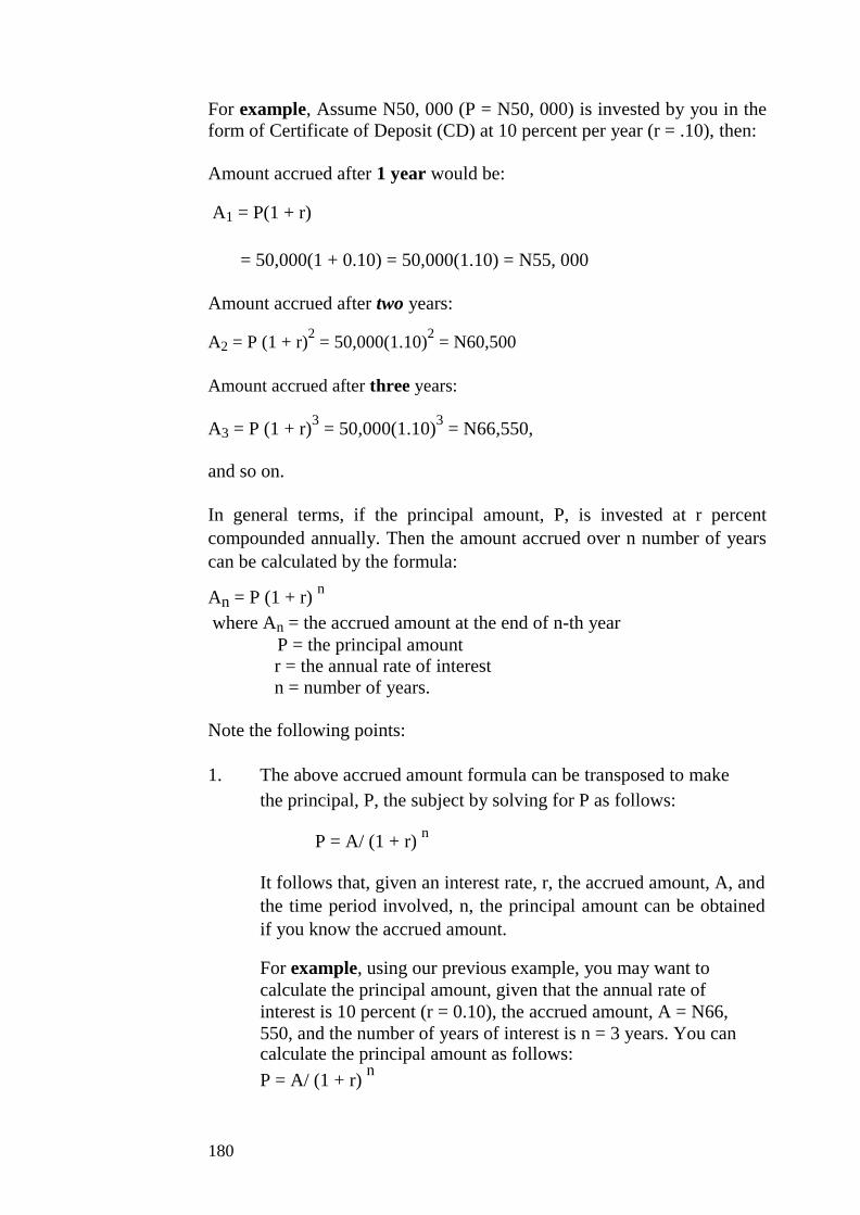
For example, Assume N50, 000 (P = N50, 000) is invested by you in the

form of Certificate of Deposit (CD) at 10 percent per year (r = .10), then:

Amount accrued after 1 year would be:

A1 = P(1 + r)

= 50,000(1 + 0.10) = 50,000(1.10) = N55, 000

Amount accrued after two years:

A2 = P (1 + r)2 = 50,000(1.10)

2 = N60,500

Amount accrued after three years:

A3 = P (1 + r)3 = 50,000(1.10)

3 = N66,550,

and so on.

In general terms, if the principal amount, P, is invested at r percent

compounded annually. Then the amount accrued over n number of years

can be calculated by the formula:

An = P (1 + r) n

where An = the accrued amount at the end of n-th year

P = the principal amount r = the annual rate of interest

n = number of years.

Note the following points:

1. The above accrued amount formula can be transposed to make

the principal, P, the subject by solving for P as follows:

P = A/ (1 + r) n

It follows that, given an interest rate, r, the accrued amount, A, and

the time period involved, n, the principal amount can be obtained

if you know the accrued amount.

For example, using our previous example, you may want to

calculate the principal amount, given that the annual rate of

interest is 10 percent (r = 0.10), the accrued amount, A = N66,

550, and the number of years of interest is n = 3 years. You can calculate the principal amount as follows:

P = A/ (1 + r) n

180

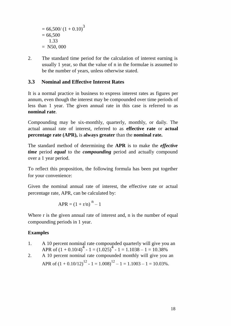
= 66,500/ (1 + 0.10)3

= 66,500

1.33

= N50, 000

2. The standard time period for the calculation of interest earning is

usually 1 year, so that the value of n in the formulae is assumed to

be the number of years, unless otherwise stated.

3.3 Nominal and Effective Interest Rates

It is a normal practice in business to express interest rates as figures per

annum, even though the interest may be compounded over time periods of

less than 1 year. The given annual rate in this case is referred to as

nominal rate.

Compounding may be six-monthly, quarterly, monthly, or daily. The

actual annual rate of interest, referred to as effective rate or actual

percentage rate (APR), is always greater than the nominal rate.

The standard method of determining the APR is to make the effective

time period equal to the compounding period and actually compound

over a 1 year period.

To reflect this proposition, the following formula has been put together

for your convenience:

Given the nominal annual rate of interest, the effective rate or actual

percentage rate, APR, can be calculated by:

APR = (1 + r/n) n – 1

Where r is the given annual rate of interest and, n is the number of equal

compounding periods in 1 year.

Examples

1. A 10 percent nominal rate compounded quarterly will give you an

APR of (1 + 0.10/4)4 - 1 = (1.025)

4 - 1 = 1.1038 – 1 = 10.38%

2. A 10 percent nominal rate compounded monthly will give you an

APR of (1 + 0.10/12)12

- 1 = 1.008)12

– 1 = 1.1003 – 1 = 10.03%.

18

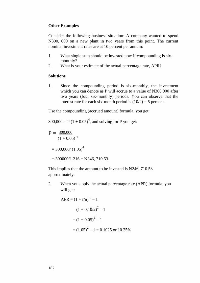
Other Examples

Consider the following business situation: A company wanted to spend

N300, 000 on a new plant in two years from this point. The current

nominal investment rates are at 10 percent per annum:

1. What single sum should be invested now if compounding is six-monthly?

2. What is your estimate of the actual percentage rate, APR?

Solutions

1. Since the compounding period is six-monthly, the investment

which you can denote as P will accrue to a value of N300,000 after

two years (four six-monthly) periods. You can observe that the

interest rate for each six-month period is (10/2) = 5 percent.

Use the compounding (accrued amount) formula, you get:

300,000 = P (1 + 0.05)4, and solving for P you get:

P = 300,000

(1 + 0.05) 4

= 300,000/ (1.05)4

= 300000/1.216 = N246, 710.53.

This implies that the amount to be invested is N246, 710.53

approximately.

2. When you apply the actual percentage rate (APR) formula, you

will get:

APR = (1 + r/n) n – 1

= (1 + 0.10/2)2 – 1

= (1 + 0.05)2 – 1

= (1.05)2 – 1 = 0.1025 or 10.25%

182

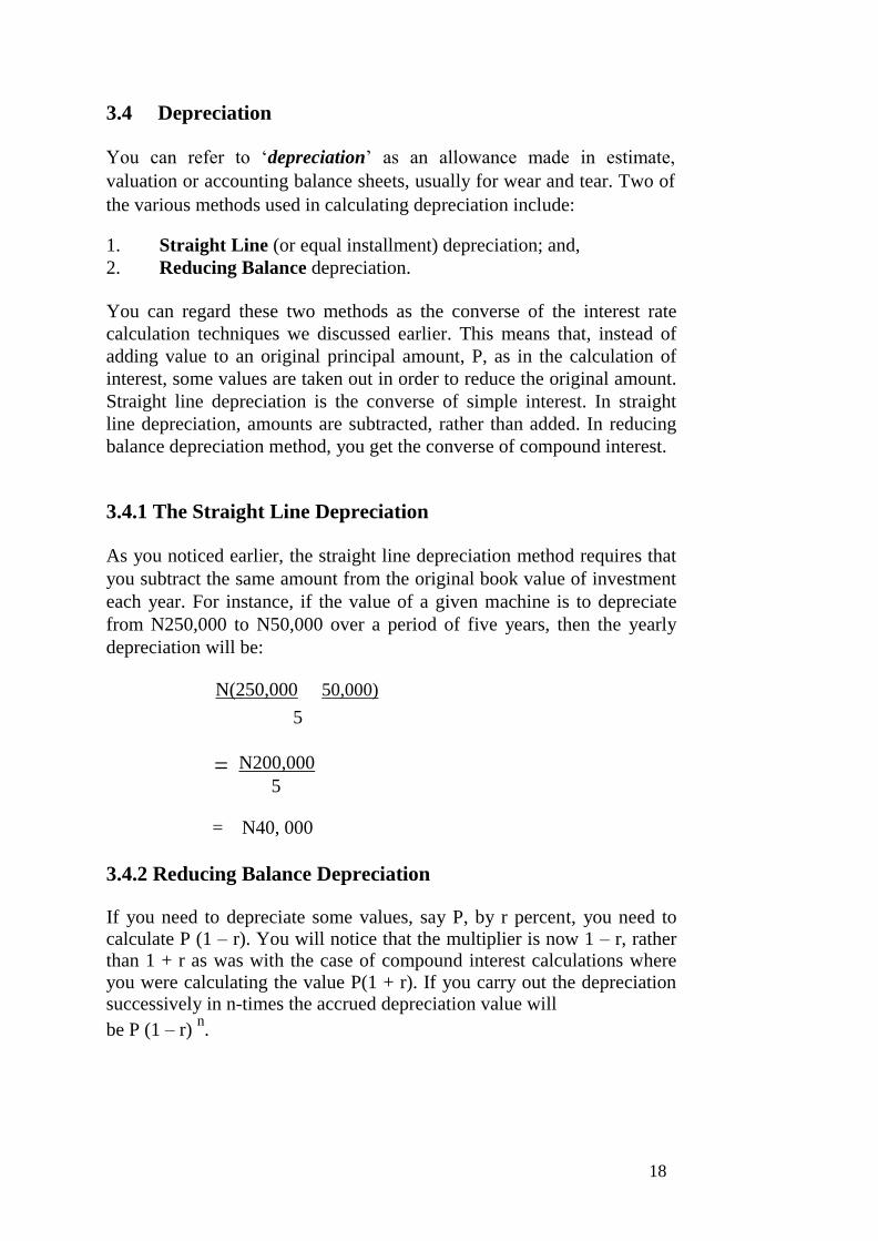
3.4 Depreciation

You can refer to ‘depreciation’ as an allowance made in estimate,

valuation or accounting balance sheets, usually for wear and tear. Two of

the various methods used in calculating depreciation include:

1. Straight Line (or equal installment) depreciation; and, 2. Reducing Balance depreciation.

You can regard these two methods as the converse of the interest rate

calculation techniques we discussed earlier. This means that, instead of

adding value to an original principal amount, P, as in the calculation of

interest, some values are taken out in order to reduce the original amount.

Straight line depreciation is the converse of simple interest. In straight

line depreciation, amounts are subtracted, rather than added. In reducing

balance depreciation method, you get the converse of compound interest.

3.4.1 The Straight Line Depreciation

As you noticed earlier, the straight line depreciation method requires that

you subtract the same amount from the original book value of investment

each year. For instance, if the value of a given machine is to depreciate

from N250,000 to N50,000 over a period of five years, then the yearly

depreciation will be:

N(250,000 50,000)

5

= N200,000 5

= N40, 000

3.4.2 Reducing Balance Depreciation

If you need to depreciate some values, say P, by r percent, you need to

calculate P (1 – r). You will notice that the multiplier is now 1 – r, rather than 1 + r as was with the case of compound interest calculations where

you were calculating the value P(1 + r). If you carry out the depreciation successively in n-times the accrued depreciation value will

be P (1 – r) n.

18

For example, if N250, 000 is depreciated by you by 10 percent (r =

0.10), over four time periods (n = 4), your final depreciated value will

be:

N {250,000(1 – 0.10)4

} = N {250,000(0.90)4}

= N164, 025.

The formula for reducing balance depreciation can be written as follows:

D = P (1 – r) n

Where D = depreciated value at the end of the n-th time period

P = the original book value r = depreciation rate

n = number of time periods, normally in years.


1. If the sum of N560, 000 is invested at 16 percent simple interest.

How much would have accrued after 8 years? 2. Find the amount of:

(a) N150, 000 compounded at 15 percent over 4 years (b) N200, 000 compounded at 12.5 percent over 7 years.

4.0 CONCLUSION

This unit has revealed that interest rate and depreciation are fundamental

concepts in business and economics. Interest is earned on money you

invested and paid on money you borrowed. To discuss interest rates and

depreciation in an understandable manner, you need to understand the

principles behind progressions, and the differences between simple and

compound interest. This and the immediate past unit have put these issues

together for you to understand.

The unit also points out that the standard time period for the calculation of

interest earning is usually 1 year, so that the value of n in the interest rate

formulae is assumed to be the number of years, unless otherwise stated.

It is a normal practice in business to express interest rates as figures per

annum, even though the interest may be compounded over time periods of

less than 1 year. The given annual rate in this case is referred to as

nominal rate.

184

Compounding may be six-monthly, quarterly, monthly, or daily, and, the

actual annual rate of interest, referred to as effective rate or actual

percentage rate (APR), is always greater than the nominal rate.

The standard method of determining the APR is to make the effective

time period equal to the compounding period and actually compound

over a 1 year period.

5.0 SUMMARY

The major issues presented in this unit can be summarised as follows:

1. In simple interest calculations, interest earned are not added back

to a principal amount, while in compound interest calculation,

interest earned is added back to the previously accrued amount

2. The actual percentage rate of interest (APR) is always greater than

the nominal rate and is formulated by:

APR = (1 + r/n) n – 1.

The term “depreciation” refers to an amount made in estimate, valuation

or accounting balance sheet. There are two major techniques employed in

the calculation of depreciation, including:

1. The straight line depreciation technique, requiring that you subtract

some amount from the original book value of a given investment

each year. 2. Reducing balance depreciation, which is a direct opposite of the

computational process for compounding interest. The formula for

this type of depreciation is worth noting again:

D = P (1 – r) n = the depreciated value at end of the n-th time

period.


A business firm invests N400, 000 per year (at the end of every year) at

15 percent compounded to meet a fixed obligation at a particular time

period. If the obligation is N800, 000 to be paid in exactly three years

from now, what single sum to be invested now needs to be added in

order to meet the obligation.



edition


18

UNIT 3 PRESENT VALUE AND INVESTMENT

APPRAISALS

CONTENTS

1.0 Introduction

2.0 Objectives

3.0 Main Content

3.1 Calculation of the Present Value

3.2 Present Value of an Interest-Bearing Debt

3.3 Capital Investment Appraisals

3.3.1 Discounted Cash Flow

3.3.2 The Internal Rate of Return (IRR)

3.4 Comparisons of Different Projects and Different Appraisal

Techniques

3.4.1 Comparison of Projects

3.4.2 Comparison of Appraisal Techniques

4.0 Conclusion

5.0 Summary



1.0 INTRODUCTION

The technique of present value and how it can be applied to future cash

flows in order to find their worth in today’s money value are becoming

essential for any productive real investment outlays. The concept ‘Present

Value’ enables businesses calculate discounted cash flows for

investments. Another important tool needed for investment decision is

that of investment appraisal method. In this unit, these issues will be

thoroughly addressed, with the aim of acquainting you with the basic

tools of investment appraisals.

2.0 OBJECTIVES


describe the present value concept

discuss investment appraisal techniques

calculate present values

define capital investments and the discounted cash

flow identify concept of internal rate of return (IRR)

explain profitable investment decisions.

186

3.0 MAIN CONTENT

3.1 Calculation of the Present Value

You can imagine that some money is invested at 10 percent per year.

Then, you can invest N10, 000 and earn N1000 in one year time period,

and your investment will be worth N11, 000. Or put it differently, the

value of N11, 000 in one year time is exactly the same as N10, 000 now.

This exemplifies the concept of the present value of a future sum.

To state this precisely, if the current investment rate is 10 percent, then

the present value of N11, 000 in one year’s time would be:

N (11,000/1.1) = N10, 000

Similarly, the present value of N20, 000 in two years time would be:

N (20,000/(1.1)2 = N16,528.93, and so on.

The investment rate, which is 10 percent in this illustration, is referred to

as the discount rate. The technique for calculation of present value can

be generalised using the following formula:

The present value of an amount NA, payable in n year’s time, subject to a

discount rate of r percent can be obtained by:

PV = A/ (1 + r)n,

Where PV = present value A = amount payable in n year’s time

r = the discount rate

n = the number of time periods in years.

The term in the above formula, A/ (1 + r) n is known as the present value

factor or the discount factor.

3.2 Present Value of an Interest-Bearing Debt

The amount of money borrowed by you will always attract interest at an

appropriate borrowing rate. Assuming there are no intermediate payments

made by you, at the end of the period involved, the amount of debt plus

the interest must be repaid by you as a lump sum. This requires the

calculation of present value of such amount.

Thus, given that the amount borrowed is say, P at r percent interest

compounded for n years, this debt will amount to P(1 + r)n. If the

investment or discount rate is j percent, the debt amount would have to

18

be discounted at j percent back over the n years. Thus the present value

of the interest-bearing debt is given by the formula:

PV = P(1 + r) n

(1 + j) n

Where r = the borrowing rate

j = the discount rate

P = the original amount borrowed

n = the number of time periods.

Note that the borrowing rate will always be greater than the investment

rate, that is, r > j, so that the ratio:

P(1 + r) n

(1 + j) n

will always be greater than 1. This is to say that the present value of the

debt (PV) will always be greater than P (the original amount borrowed).

Example

Can you find the present value of a debt valued at N250, 000 taken out

over 3 years, with no intermediate payments, given that the borrowing

rate is 15 percent per year and the discount rate or the worth of money is

10 percent.

Solution

The maturity value of the debt will be calculated as:

P (1 + r)3 = 250,000(1 + 0.15)

3 = N[250,000(1.15)

3] =

N3802,218.75 Therefore, the present value becomes:

PV = 3,802,218.75

(1.10)3

= N2, 856,663.22

This means that the original debt of N250, 000 will cost (in today’s

monetary terms) N2, 856,663.22 to repay.

188

3.3 Capital Investment Appraisals

In its simplest form, capital investment is a project consisting of:

(i) an initial outlay

(ii) a set of estimated cash inflows and outflows over the life of the

project

(iii) optionally, a resettlement figure which might be as a result of plant

resale or shares, or cash settlement for clearing any liabilities in the

cause of project execution.

There are many ways you can appraise and compare capital investments,

but we look at two ways or techniques, both using the concept of

discounting, including:

1. Discounted Cash Flow 2. Internal Rate of Return (IRR).

3.3.1 Discounted Cash Flow

The discounted cash flow technique involves calculating the sum of the

present values of all cash flows associated with an investment project.

This sum is referred to as the Net Present Value (NPV) of the project.

The cash flows are tabulated net per year. The standard presentation

format is illustrated by the example that follows.

Example

Assume that a business project is being considered, with initial costs of

N12,000 and corresponding revenues or inflows over the following 4

years of N8,000, N12,000, N10,000, and N6,500, respectively. If the

project costs (outflows) over the 4 years are estimated at N8,500, N3,000,

N1,500, and N1,500, respectively, and the discount rate is 10 percent,

evaluate the project’s Net Present Value (NPV).

Solution

Tables 18.1 and 18.2 below present the project’s cash flows and the

discounted cash flows respectively. Table 18.2 yields the net present

value of the project.

18

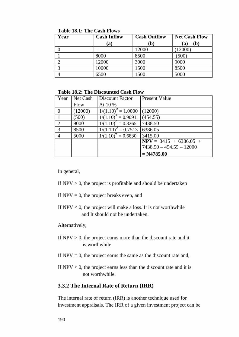
Table 18.1: The Cash Flows Year Cash Inflow Cash Outflow Net Cash Flow

(a) (b) (a) – (b)

0 - 12000 (12000)

1 8000 8500 (500)

2 12000 3000 9000

3 10000 1500 8500

4 6500 1500 5000

Table 18.2: The Discounted Cash Flow Year Net Cash Discount Factor Present Value

Flow At 10 %

0 (12000) 1/(1.10)0 = 1.0000 (12000)

1 (500) 1/(1.10)1 = 0.9091 (454.55)

2 9000 1/(1.10)2 = 0.8265 7438.50

3 8500 1/(1.10)3 = 0.7513 6386.05

4 5000 1/(1.10)4 = 0.6830 3415.00

NPV = 3415 + 6386.05 + 7438.50 – 454.55 – 12000

= N4785.00

In general,

If NPV > 0, the project is profitable and should be undertaken

If NPV = 0, the project breaks even, and

If NPV < 0, the project will make a loss. It is not worthwhile

and It should not be undertaken.

Alternatively,

If NPV > 0, the project earns more than the discount rate and it

is worthwhile

If NPV = 0, the project earns the same as the discount rate and,

If NPV < 0, the project earns less than the discount rate and it is

not worthwhile.

3.3.2 The Internal Rate of Return (IRR)

The internal rate of return (IRR) is another technique used for

investment appraisals. The IRR of a given investment project can be

190

defined as the value of the discount rate that gives a zero Net Present

Value (NPV), (that is, NPV = 0). The internal rate of return can also be

viewed as the rate earned by a given project.

Presently, there does not exist a precise formula for calculating the

internal rate of return for a project. Nevertheless, IRR can be estimated

using a linear interpolation formula as presented below:

IRR = N

1

R 2

- N 2

R 1

N1 - N 2

Where the discount rate, R1 gives NPV of N1, and the discount rate R2

gives NPV of N2

Example

Let the discount rate, R1 = 15% yield an NPV of N140, 000 (that is,

R1 = 0.15 and N1 = 140,000); and, the discount rate of R2 = 17% yield

an NPV of -N70, 000 ( R2 = 0.17 and N 2 = -70,000). It follows that:

IRR = (140,000)(0.17) - (-70,000)(0.15)

140,000 - (-70,000)

= 23,800 + 10,500 140,000 + 70,000)

= 34,300

210,000

= 0.1633 or 16.33 percent.

Therefore, the estimate of the internal rate of return (IRR) is

approximately 16.33 percent. This is the discount rate that yields NPV =

0.

In the following example, you will see the use of the above formula from

a discount cash flow table.

Example

Using table 18.3 below, we wish to calculate the NPV corresponding to

each of two discount rates, 6 percent and 9 percent, summing up to 15

percent. We also estimate the internal rate of return of the project.

19

Solution

When calculating the NPVs of a project using two separate discount rates,

you should combine both sets of calculations into a single table. This dual

discounted cash flow table for the project is presented in table 18.3

below.

Table 18.3: The Dual Discounted Cash Flow

Year Net Flow Discount Present Discount Present

factor at Value factor at Value

6% 9%

0 (60,000) 1.0000 (60,000) 1.0000 (60,000)

1 (10,000) 0.9434 (9,434) 0.9174 (9174)

2 15,000 0.8900 13,350 0.8417 12,625.50

3 20,000 0.8396 16,792 0.7722 15,444

4 20,000 0.7921 15,842 0.7084 14,168

5 20,000 0.7473 14,946 0.6499 12,998

6 20,000 0.7050 14,100 0.5963 11,926

NPV 5,596 (2,012.50)

Using the formula, we estimate the IRR as follows:

IRR = N1 R 2 - N 2 R 1

N1 - N 2

Where N1 = 5596; N2 = -2,012.50;

R1 = 0.06; R2 = 0.09

IRR = (5596)(0.09) ( 2012.50)(0.06)

5596 ) 2012.50)

= 503.64 + 120.75

5569 + 2012.50

= 524.39

7608.50

= 0.082065

= 0.0821 or 8.21 percent.

192

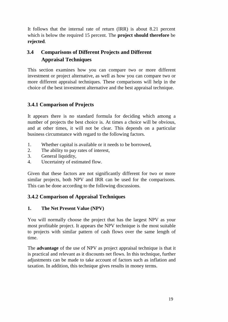
It follows that the internal rate of return (IRR) is about 8.21 percent

which is below the required 15 percent. The project should therefore be

rejected.

3.4 Comparisons of Different Projects and Different

Appraisal Techniques

This section examines how you can compare two or more different

investment or project alternative, as well as how you can compare two or

more different appraisal techniques. These comparisons will help in the

choice of the best investment alternative and the best appraisal technique.

3.4.1 Comparison of Projects

It appears there is no standard formula for deciding which among a

number of projects the best choice is. At times a choice will be obvious,

and at other times, it will not be clear. This depends on a particular

business circumstance with regard to the following factors.

1. Whether capital is available or it needs to be borrowed, 2. The ability to pay rates of interest,

3. General liquidity, 4. Uncertainty of estimated flow.

Given that these factors are not significantly different for two or more

similar projects, both NPV and IRR can be used for the comparisons.

This can be done according to the following discussions.

3.4.2 Comparison of Appraisal Techniques

1. The Net Present Value (NPV)

You will normally choose the project that has the largest NPV as your

most profitable project. It appears the NPV technique is the most suitable

to projects with similar pattern of cash flows over the same length of

time.

The advantage of the use of NPV as project appraisal technique is that it

is practical and relevant as it discounts net flows. In this technique, further

adjustments can be made to take account of factors such as inflation and

taxation. In addition, this technique gives results in money terms.

19

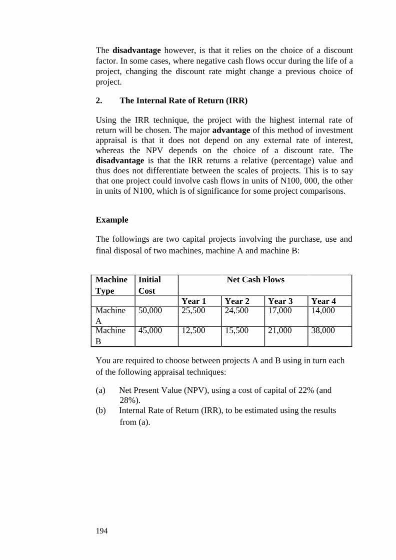
The disadvantage however, is that it relies on the choice of a discount

factor. In some cases, where negative cash flows occur during the life of a

project, changing the discount rate might change a previous choice of

project.

2. The Internal Rate of Return (IRR)

Using the IRR technique, the project with the highest internal rate of

return will be chosen. The major advantage of this method of investment

appraisal is that it does not depend on any external rate of interest,

whereas the NPV depends on the choice of a discount rate. The

disadvantage is that the IRR returns a relative (percentage) value and

thus does not differentiate between the scales of projects. This is to say

that one project could involve cash flows in units of N100, 000, the other

in units of N100, which is of significance for some project comparisons.

Example

The followings are two capital projects involving the purchase, use and

final disposal of two machines, machine A and machine B:

Machine Initial Net Cash Flows

Type Cost

Year 1 Year 2 Year 3 Year 4 Machine 50,000 25,500 24,500 17,000 14,000

A Machine 45,000 12,500 15,500 21,000 38,000

B

You are required to choose between projects A and B using in turn each

of the following appraisal techniques:

(a) Net Present Value (NPV), using a cost of capital of 22% (and

28%). (b) Internal Rate of Return (IRR), to be estimated using the results

from (a).

194

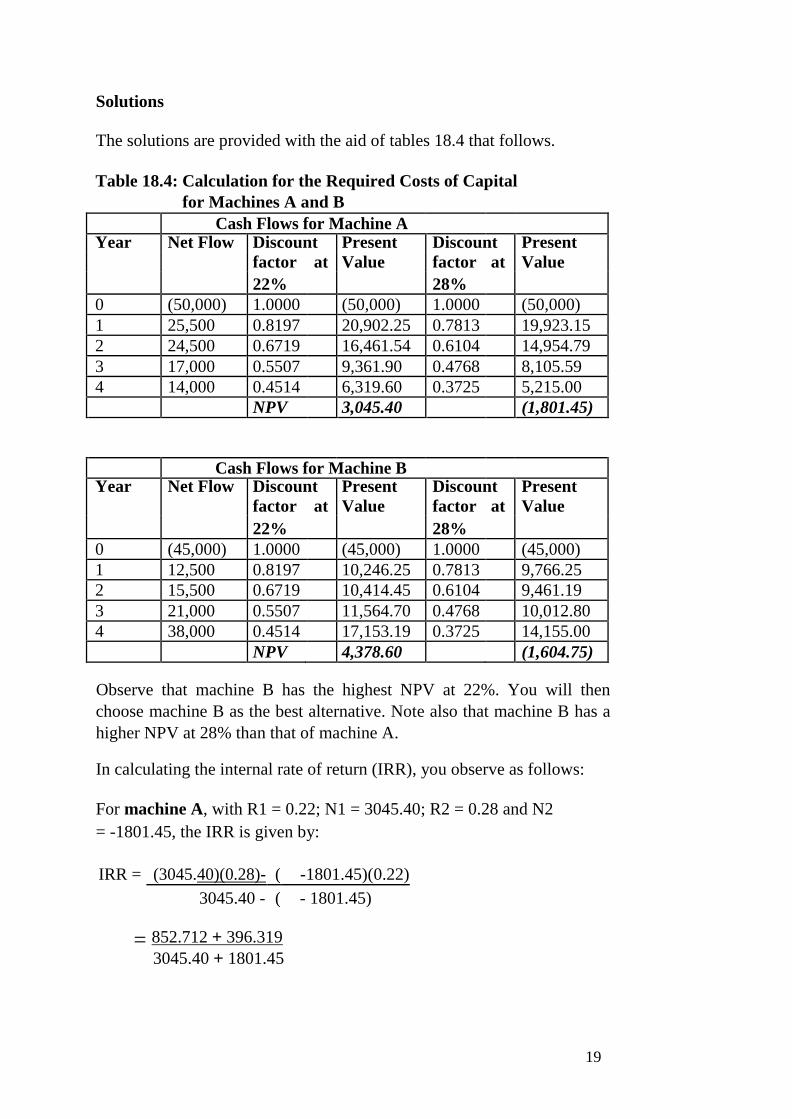
Solutions

The solutions are provided with the aid of tables 18.4 that follows.

Table 18.4: Calculation for the Required Costs of Capital

for Machines A and B

Cash Flows for Machine A



22% 28%

0 (50,000) 1.0000 (50,000) 1.0000 (50,000)

1 25,500 0.8197 20,902.25 0.7813 19,923.15

2 24,500 0.6719 16,461.54 0.6104 14,954.79

3 17,000 0.5507 9,361.90 0.4768 8,105.59

4 14,000 0.4514 6,319.60 0.3725 5,215.00

NPV 3,045.40 (1,801.45)

Cash Flows for Machine B



22% 28%

0 (45,000) 1.0000 (45,000) 1.0000 (45,000)

1 12,500 0.8197 10,246.25 0.7813 9,766.25

2 15,500 0.6719 10,414.45 0.6104 9,461.19

3 21,000 0.5507 11,564.70 0.4768 10,012.80

4 38,000 0.4514 17,153.19 0.3725 14,155.00

NPV 4,378.60 (1,604.75)

Observe that machine B has the highest NPV at 22%. You will then

choose machine B as the best alternative. Note also that machine B has a

higher NPV at 28% than that of machine A.

In calculating the internal rate of return (IRR), you observe as follows:

For machine A, with R1 = 0.22; N1 = 3045.40; R2 = 0.28 and N2

= -1801.45, the IRR is given by:

IRR = (3045.40)(0.28)- ( -1801.45)(0.22)

3045.40 - ( - 1801.45)

= 852.712 + 396.319 3045.40 + 1801.45

19

= 1249.031

4846.85

= 0.2577 or 25.8 percent

For machine B, with R1 = 0.22; N1 = 4378.60; R2 = 0.28; N2

= -1604.75, the IRR is given by:

IRR = (4378.60)(0.28)- (- 1604.75)(0.22)

4378.60- (- 1604.75)

= 1226.01 + 3530.5 4376.6 + 1604.70

= 1579.06

5981.30

= 0.264 or 26.4 percent.

It follows that machine B has a higher rate of return (IRR = 26.4%) than

machine A, with IRR = 25.8%. Overall, machine B is clearly the best

choice.


1. What do you understand by Net Present Value (NPV) and

Internal Rate of Return (IRR)? How are they used? 2. Why do you think it is useful to know the present value of an

interest-bearing debt? 3. What are the basic methods available for appraising and

comparing capital investments?

4.0 CONCLUSION

This unit has brought to bear the technique of present value and how it

can be applied to future cash flows in order to find their worth in today’s

money value. We noted that this is highly essential for any productive real

investment outlays. The concept ‘Present Value’ enables businesses

calculate discounted cash flows for investments. Another important tool

needed for investment decision is that of investment appraisal method.

There are two basic investment appraisal techniques including, the net

present value (NPV) and the internal rate of return (IRR). We discovered

that the best choice of investment alternative is the alternative with either

the highest NPV or the highest IRR or both as the case maybe.

196

5.0 SUMMARY

The information you obtained from unit 16 can be summarised as

follows:

1. The present value (PV) technique enables you obtain a future cash

flow which will be equivalent to today’s monetary value. The

present value is obtained by multiplying the cash flow by a

discount factor. 2. The present value of an interest bearing debt can be obtained by:

(a) compounding the debt over an appropriate time period,

using an appropriate borrowing rate;

(b) discounting back to today, using an appropriate

investment rate. 3. The Net Present Value (NPV) of a project can be obtained by

discounting all cash flows and adding them together, and:

If NPV > 0, the project will be profitable

If NPV = 0, the project breaks even

If NPV < 0, the project is not profitable and not worthwhile.

4. The internal rate of return (IRR) of a project is that discount rate

for which the NPV = 0. It is the rate of interest earned by a given

project. 5. Investment appraisals using discounting techniques involves

considering the worth of one or more capital projects, using either

net present value (NPV) or internal rate of return (IRR).


A business outfit is considering borrowing N100, 000 to invest in a

project, which is expected to yield N350, 000 at the end of each of the

next 5 years. If the cost of capital is 25 percent:

(a) draw up a discount cash flow table and calculate the NPVs of the

project. (b) interpret your calculated value of NPV in light of the given

situation.



edition


UNIT 4 NATURE OF STATISTICS

CONTENTS

1.0 Introduction

2.0 Objectives

3.0 Main Content

3.1 Definitions

3.2 Classification of Data

3.3 Types of Statistics

3.4 Use of Statistical Data

3.5 Sources of Data Collection

3.5.1 Methods of Collection of Data

3.5.2 Types of Data Collection

3.5.3 Errors in Data Collection

3.5.4 Problems of Data Collection

3.6 Essential Steps Involved in Sample Survey

3.7 Steps Involved in Solving Statistical Problem

4.0 Conclusion

5.0 Summary



1.0 INTRODUCTION Statistics is an intensive field of study which stems from the study of probability,

resulting from information gathering. Therefore, in this unit, you will learn how you

can use statistics to investigate and analyse data. You will, surely find this to be a

rewarding experience.

2.0 OBJECTIVES

At the end of the unit, you should be able to:

define statistics

state basic statistical terms

describe data collection processes

explain how to write a good questionnaire.

3.0 MAIN CONTENT

3.1 Definitions

Here, let us look at the following concepts.

Statistics- This is concerned with scientific methods and theories which deals with

data collection, organisation, summarisation, presentation, analysis, interpretation and

utilisation of the results to draw useful conclusions, in order to make reasonable

decisions.

Statistic- This is a numerical quantity whose values can be gotten from a sample data

e.g. mean, median and mode of a data.

Data- These are facts, bits of information or series of observations that are obtained

from an investigation. These facts can be measured or quantified.

Information- This is knowledge given. It is, necessarily, obtained from investigation

or observation, and cannot always be measured or quantified.

Data set- These are data collected from a particular investigation or study.

Statistical data- These data are bits of information or measurements that are collected

in the process of an investigation or observation.

3.2 Classification of Data Data can be classified into two.

1. Numerical data

2. Non-numerical data

Numerical data- Numerical data consist of values that can be quantified. They can be

divided into discrete continuous data.

Discrete data- These are numerical data that consist of values that cannot assume

values between two given values. They can only assume a particular value. Discrete

data are whole numbers which can be positive, negative or zero integers, but does not

include factions or decimal numbers. For example, ‘the number of books in the book

shelves can either be 0, 1, 2…and not 3½ or 4.6 5 3’.

Continuous data- these are numerical data which can assume values between two

given values. They can be positive integers, negative integers or zero, fractions or

decimals. Example of continuous data includes weight of items, height of pupils in a

school age of individuals. In general, measurement gives rise to continuous data, while

enumeration or counting gives rise to discrete data.

Non-numerical data- these are data which the value cannot be quantified. Examples

are skin colour, nationality, gender, marital status, income group etc.; non- numerical

data can also be divided into ordinal and categorical data.

Ordinal data-these are non-numerical data which the values can be arranged in an

ordinal scale. They cannot be measured in natural numerical scale. Examples are

income group, age group, classmate, boxers’ weight, and academic grades. Academic

grade is a label (an “A” grade student) that also belongs to a ranking system (“A” is

better than “B”)

Categorical data-These are non-numerical data which the values can only be put in

categories. They cannot be arranged in an ordinal scale, but their measurement can be

recorded on a natural occurring numerical scale. Examples are marital status,

nationality, gender, religion, etc.

Variable-This is a quantity that varies, the opposite of a constant e.g. the numbers of

customers that enters a shopping mall per hour varies, but the number of minutes per

hour is constant. Value-A value is a specific amount that a variable could be; for example-‘the number of

callers to a call centre, in the last one hour, is 40’.

Observation or observed values- This is a value of a variable that has actually

occurred or has been counted or measured.

3.3 Types of Statistics

Statistics, by nature, can be divided into two groups:

1. Descriptive or deductive statistics

2. Inductive or inferential statistics.

Descriptive statistics- This can also be referred to as deductive statistics; and it is the

phase of statistics which seeks only to describe and analyse a given group without

drawing any conclusions or inferences about a large group (population). Descriptive

statistics covers areas such as mean, median, mode, standard deviation etc., and can be

presented in form of graph, data, tables, charts and other statistical tools. Example-‘the

classification of the graduates of PGD students of Chartered Institute of Shipping

(CIS) according to their sex, courses and G.P.A., without drawing any conclusion or

inference about the graduates is descriptive statistics.

Inductive statistics- this can also be called inferential statistics and it is that phase of

statistics which enables one to draw conclusions or inferences about a large group,

(population) from the analysis of sample drawn from the population. Most often, it is

cumbersome and almost impossible to observe or collect data from the entire

population; as a result, a part of the population- known as a representative sample, is

considered, which represents the characteristics of the population. If the sample drawn

is a true representative of the population, upon analysis of the observed sample, one

can make inference about the population. The condition under which such inference is

valid is inductive or inferential statistics.

3.4 Use of Statistical Data Statistics plays a very vital role in day- to-day activities of man. Every field of life-

ranging from business, account, banking, insurance, agriculture, energy, industry,

science, engineering to medicine, make use of statistics. Some of the ways statistics

has been found to be useful are as listed below.

1. It is used for effective budgeting, planning and forecasting future growth

2. It is used to summarise large data into concise information

3. It is used for the purpose of estimation and prediction of government revenue and

expenditure

4. It is used for formulating policies for developmental purpose

5. It is used for both short and long-term forecast of future events

6. It is used in industries to control production process

7. It is used for making conclusions from data collected in experimental, social and

behavioural research Organisations use statistics to evaluate and monitor performance

8. It plays an important role in the usage of computers.

3.5 Sources of Data Collection

Sources of data, among numerous others, include the following.

Agricultural statistics and data- This contains agricultural statistics and data.

Crime statistics and data- This provides varieties of criminal justice statistics and

data archives.

Demographic data- This deals with population, fertility and mortality data.

Economic growth data- This data is useful in conducting studies of economic growth.

Educational statistics and data- This deals with high school and college

environments, educational cost, public sector investment and related information.

Questionnaires- These are popular means of collecting data, where questions are

designed to get responses from respondents and the result of the responses are coded,

quantitatively, for the purpose of analysis and interpretation.

Health data- This provides information on health care etc.

3.5.1 Methods of Collection of Data Data collection can be seen as a means of gathering or obtaining information from

selected sample of investigation. Without data collection, analysis cannot be done, and

hence, meaningful planning and decision-making will be impossible. Therefore

collection of data serves as required fact finding for any statistical analysis. Data

collection enables us to evaluate numerical data and verify claims made about such

data. It also helps in measuring the reliability of our inferences. There are six methods

of data collection, as itemised below.

Experimental method

Direct observation

Personal interview

Telephone survey

Registration

Questionnaire

Experimental method- This is the method used in science laboratory to collect

information. Here, data is obtained from laboratory experiments, and the results are

recorded immediately.

Direct observation: This is a method of data collection, whereby the investigator

watches and records what actually happens. The data collected here are more reliable

and dependable. Data collected in this manner does not give information about the past

or future; it only gives information about the present.

Personal interview-This is a method whereby the interviewer and the respondent

(interviewee) have a direct contact during the process of interview. Direct contact can

be in form of face-to-face, one-on-one, ‘many-to-one, or one-to-many. Advantages

The interviewer can re-frame and explain unclear questions to the interviewee.

The data collected are original and direct from source.

It reduces ambiguity. Disadvantages

It is expensive and time consuming.

There is the possibility of personal bias.

Telephone survey method- this is an oral interview via the telephone; this method is

easy and convenient, but does not put into consideration those respondents that do not

have access to telephone. Advantages

It is convenient and fast

It has a wide coverage. Disadvantages

It is expensive and exclusively for the rich.

The respondent may refuse to respond to the interviewer.

Registration method- This is the method of data collection whereby information is

collected through registration. Example of data collection by registration method

includes birth registration, marriage registration, and death registration. Advantages

It is easy and saves time.

It reduces cost, especially, in carrying out census.

It gives estimate of population.

Questionnaire method- This is a method whereby a carefully, well organised questions-

on all the information needed for an investigation, are written or printed and distributed

to intended respondents for their responses. There are two types of questionnaires,

namely:

Self-administered questionnaire

Mail/postal questionnaire

Self administered questionnaire-This is a method of data collection which involves

distribution of questionnaire to the respondents to obtain the needed information,

immediately.

Mail/postal questionnaire-This involves sending the questionnaire by mail/post to

respondents. This technique often covers a wild geographical area, and it is mostly

used when respondents are scattered. However, this method is not as effective as self

administered questionnaires, in that the respondent may refuse to send back the

questionnaire to the interviewer; and the questionnaire could also be lost in transit.

Advantages

It is cheap.

It provides room for privacy as the respondent feels free to answer some

questions.

It covers wide geographical area.

It is free of any possible bias from the interviewer.

Disadvantages

There could be loss of questionnaire in transit.

Refusal to send back the questionnaire.

The respondent may not have the required information. This is highly possible

in an environment with high illiteracy level.

Designing a good questionnaire - a good questionnaire must be designed in such a

way that it will reflect all the information needed for the study at hand. A badly

designed questionnaire may ruin a well planned survey. Most importantly, questions

and answers are the means of communication between the investigator and

respondents; hence, the respondent, therefore, remains the only source of information

available for decision-making. As a result, there are a number of rules we must follow,

as a guide, when designing a questionnaire; these are as follows.

The questions must be short, direct and easy to understand.

The questions must not be difficult or ambiguous.

Avoid questions that lead to a particular answer; e.g. ask- “which brand of beverage do

you consider the best?” and not- “do you consider Milo to be the best brand of

beverage?”, mentioning a name can lead to a particular answer. Ensure that the

respondent has the information. The questionnaire must be properly edited and be in

order, so as to give room for completeness, consistency and homogeneity. The

questions must not be personal or offensive. Consider if the respondent will be willing

to tell the truth, if telling the truth can affect his personality and integrity.

3.5.2 Types of Data Collection

There are, basically, two main types of data collection, these are listed below.

Primary data

Secondary data

Primary data

Data is collected from a representative sample for a particular study or investigation,

for a particular purpose by means of sample survey; data collected are used for the

purpose for which they are collected. Primary data is the most advisable to use in

statistical analysis, because of its accuracy, reliability and dependability in decision-

making.

Advantages

The purpose of collection is as follows.

Sorting out is possible; that is, the part of the data that are not relevant to the

study can be removed or ignored.

Sampling procedure is known.

Disadvantages

It is expensive to carry out.

It involves a lot of steps, especially, in a large survey.

Sorting out must be done before analysis.

Sorting out may be cumbersome, especially, in large survey.

Secondary data

This relates to data which already exists, and which is used for a purpose other than

that for which it was collected. Secondary data are obtained from publications,

journals, records of government, dailies, and news magazines; agencies are engaged in

routine data collections. These agencies include the following;

The federal and state office of statistics

Central Bank of Nigeria

Research institutes and universities

Industries and commercial organisations

Advantages

It is cheap and easier to collect, because it is readily available.

It already existed, and it is sorted and processed.

It facilitates and speeds up analysis.

Disadvantages

Errors involved in the original collection cannot be detected and eliminated.

Its sampling procedure is not known.

It is less used, compare to primary data.

The purpose of collection is not known, and so it may not be suitable for the

investigation.

3.5.3 Errors in Data Collection Ineffective communication between the investigator and respondent- This relates

to communication gap between parties involved. Problem of difficult questions- As it has been discussed above, some questions on

questionnaires may be too difficult and unclear for respondent to understand Problem of exaggeration on the part of respondents- Some respondents may be

biased because of personal affiliation to the administrator or attendant or interview and

therefore, play prank with responses. Financial and logistic problem- The investigator may have challenges in the area of

transportation and funding; this may affect data collection, which in turn, can affect the

investigation negatively. Return of incomplete questionnaire- as respondent may skip some key questions.

When an investigator hurriedly administers questions on respondent, the respondent

may fill that the best way to satisfy the curiosity of the investigator is to quickly tick

his response, and in the process some questions are left unanswered. Respondent may not be willing to tell the truth- There is an adage that says that

“truth is always bitter”; respondents sometimes may be unwillingly to disclose the

truth, especially in an interview situation. He/she may fill that saying the right thing at

the time may be tantamount to divulging information that can implicate him/her.

Now, basically, these errors can be classified as shown below, as well. Sampling error-the sampling techniques used may not valid so as to provide

information regarding the population investigated. Transcription error- An investigator may wrongly put down wrong data which could

result to leverage points. Response errors - It is possible to give false response on questions that are not well

understood. Measurement error- It is most often observed that an investigator may use qualitative

data for quantitative data. This kind of measurement will derail the authenticity of what

is to be measured. Biased error- The investigator may be judgmental. He may have concluded in his

mind the result of the data prior to carrying out the investigation. Therefore, the sample

used may not be a representative of the parent population. Incompleteness or non-coverage area required- The design of the research work

may be faulty and thus information regarding what is to be investigated may be lost. Compilation error- even when the instruments for data collection are well planned in

advance wrong compilation may entangle the result of the investigation. Time change error- If the information or data collected is obsolete, it may not be

useful for investigation. That is, the information may not be seasoned when current

information surpasses it. Rounding error- If digits or figures are rounded wrongly they affect the data

collected. Secondary data error- the errors involve in the collection of this kind of data may be

taskful to detect since it does not originate from the researcher.

Now, from the above, you can infer that the following are the basic problems

associated with data collection.

Ineffective communication between investigator and respondents.

Problem of difficult questions.

Problem of exaggeration on the part of respondents.

Financial and logistic problems related to data collection.

Return of incomplete questionnaire as respondent may skip some key questions.

Respondents may not be willing to tell the truth.

3.6 Essential Steps Involved in Sample Survey

The following are the steps to follow in conducting a sample survey.

Definition of aims and objectives of the survey

Literature search

Development or design of questionnaire- which will reflect all the information

needed to achieve stated objectives

Determination of sample size and sampling method or technique

Total cost estimation

Pilot survey- a test run of the designed questionnaire for possible modification

Man power training

Main survey- this involves sending out trained personnel for data collection,

using the validated instruments

Post estimation survey- to check the validation of the survey results and correct

all possible errors

Survey result analysis and interpretation, using appropriate statistical technique

Survey report and conclusion.

3.7 Steps Involved in Solving Statistical Problem

Here, take note of the following

Define the problem

Search for cause of the problem

Provision of alternative solutions

Evaluation of the solution

SELF-ASSESSMENT EXERCISE

Outline 10 ways you can use statistics.

4.0 CONCLUSION

In this unit, you have learnt the best way to apply statistics in various disciplines. It has

been mentioned to you that data collection process takes two forms, namely- primary

data and secondary data. This part is very crucial to your research process; therefore,

you can now go on to apply what you have learnt in this unit. Let us examine other

aspect of statistics in the next unit which is also pertinent to your study of statistics.

5.0 SUMMARY

So far in this unit, you have learnt about the nature of statistics. Some vital areas of

statistics have been exposed to you-these include data, information, categorical and

non-categorical data and ways to write a good questionnaire. You can now proceed to

apply all that you learnt here.


What is statistics?

Distinguish between the following and give two example of each.

Numeric and non-numeric data

Discrete and continuous data

Ordinal and continuous data

Ordinal and categorical data


Adamu, I. M. (2006). Understanding Basic Statistics. Nile Ventures.

Babatunde, L. & Elegbede, W. (2005). Business Statistics: Concepts and

Application. (1st ed.). Life and Ministry Publications.

Kazmier, L. (1972). Schaum’s Outline of Theory and Problems of

Statistics. (SI Metric Edition). Singapore: McGraw Hill.

Lind, D., Marchal, W. & Wathen, S. (2010). Statistical Techniques in

Business and Economics. ( 4th ed.). McGraw-Hill.

UNIT 5 SAMPLING TECHNIQUES

CONTENTS

1.0 Introduction

2.0 Objectives

3.0 Main Content

3.1 Population

3.1.1 Sample

3.1.2 Total Enumeration

3.2 Sampling Techniques

3.2.1 Probability Sampling Technique

3.2.2 Non-Probabilistic Sampling

4.0 Conclusion

5.0 Summary



1.0 INTRODUCTION

You have just learnt about data collection techniques. However, for you

to have reliable and valid data there is need to understand the sampling

procedure that can ensure better data processing. This is within the

purview of sampling techniques.

2.0 OBJECTIVES


c) define some basic elements of sampling techniques d) explain types of sampling.

3.0 MAIN CONTENT

3.1 Population

A population is a set or collection of objects, units having similar,

observable characteristics. A population may be finite or infinite.

Finite population- the units are countable with a frame i.e. a list of all

the units.

Infinite population- this could be countable, but with an impossible

frame.

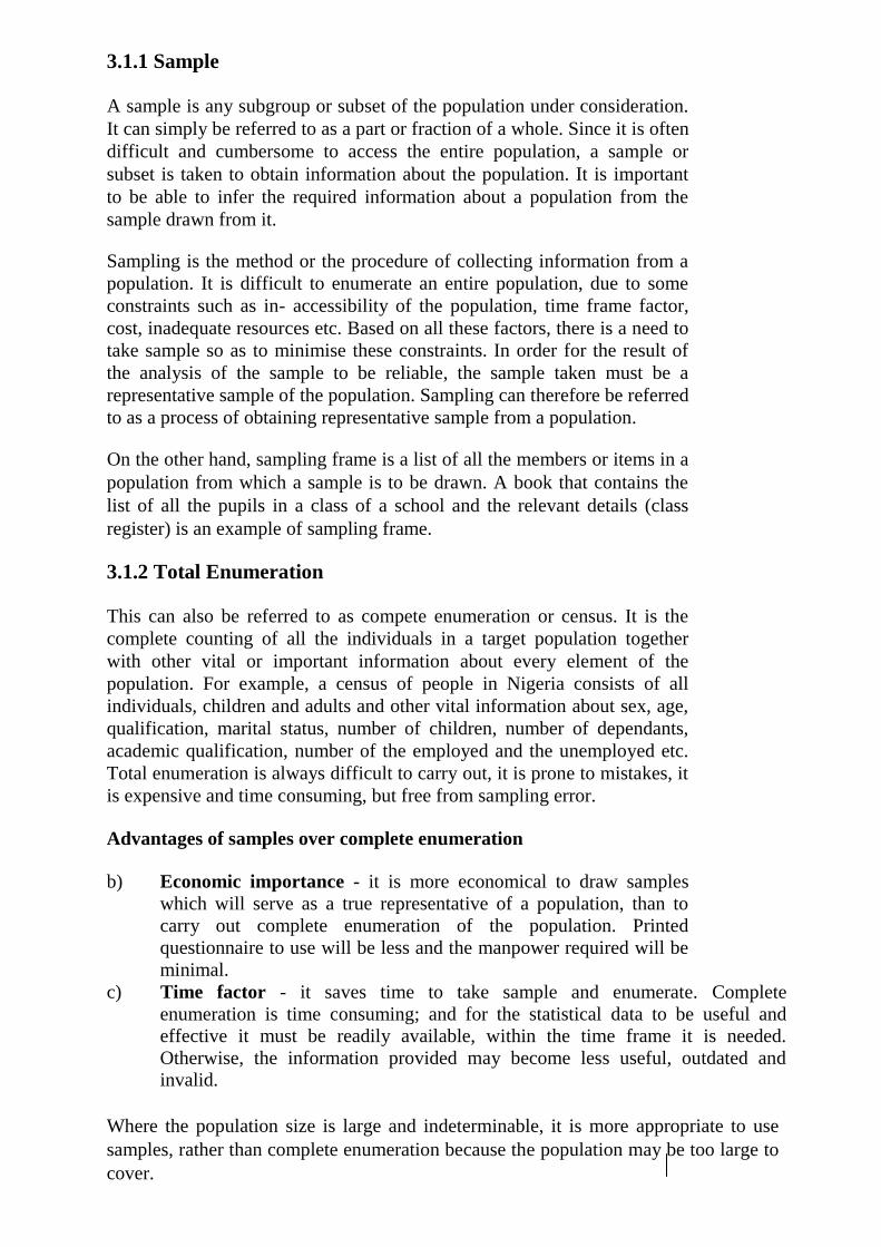
3.1.1 Sample

A sample is any subgroup or subset of the population under consideration.

It can simply be referred to as a part or fraction of a whole. Since it is often

difficult and cumbersome to access the entire population, a sample or

subset is taken to obtain information about the population. It is important

to be able to infer the required information about a population from the

sample drawn from it.

Sampling is the method or the procedure of collecting information from a

population. It is difficult to enumerate an entire population, due to some

constraints such as in- accessibility of the population, time frame factor,

cost, inadequate resources etc. Based on all these factors, there is a need to

take sample so as to minimise these constraints. In order for the result of

the analysis of the sample to be reliable, the sample taken must be a

representative sample of the population. Sampling can therefore be referred

to as a process of obtaining representative sample from a population.

On the other hand, sampling frame is a list of all the members or items in a

population from which a sample is to be drawn. A book that contains the

list of all the pupils in a class of a school and the relevant details (class

register) is an example of sampling frame.

3.1.2 Total Enumeration

This can also be referred to as compete enumeration or census. It is the

complete counting of all the individuals in a target population together

with other vital or important information about every element of the

population. For example, a census of people in Nigeria consists of all

individuals, children and adults and other vital information about sex, age,

qualification, marital status, number of children, number of dependants,

academic qualification, number of the employed and the unemployed etc.

Total enumeration is always difficult to carry out, it is prone to mistakes, it

is expensive and time consuming, but free from sampling error.

Advantages of samples over complete enumeration

b) Economic importance - it is more economical to draw samples

which will serve as a true representative of a population, than to

carry out complete enumeration of the population. Printed

questionnaire to use will be less and the manpower required will be

minimal. c) Time factor - it saves time to take sample and enumerate. Complete

enumeration is time consuming; and for the statistical data to be useful and

effective it must be readily available, within the time frame it is needed.

Otherwise, the information provided may become less useful, outdated and

invalid.

Where the population size is large and indeterminable, it is more appropriate to use

samples, rather than complete enumeration because the population may be too large to

cover.

3.2 Sampling Techniques

There are, basically, two types of sampling techniques-as shown below.

(b) Probability sampling techniques (c) Non-probability sampling techniques

TYPES OF SAMPLING

PROBABILISTIC SAMPLING NON-PROBABILISTIC SAMPLING

SIMPLE RANDOM SAMPLING

JUDGEMENT SAMPLING

STRATIFIED RANDOM SAMPLING

QUATA SAMPLING

SYSTEMATIC SAMPLING CHUNK OR CONVENECE SAMPLING

CLUSTER SAMPLING

VOLUNTEERS

MULTISTAGE SAMPLING

Fig. 2.1: Schema Showing the Typology of Sampling Techniques

3.2.1 Probability Sampling Technique

This selection is based on the use of existing probability law where each

element in the population is known. These techniques include the list

below.

1. Simple random sampling technique

2. Stratified random sampling technique

3. Systematic sampling technique

4. Cluster sampling technique

5. Multistage Sampling technique

Let us look at these one by one.

2. Simple random sampling technique This is a sampling technique in which every possible sample

(items) of size n taken from the population size N has equal and

independent chances of being chosen. The selection is not biased.

This sampling method or technique can also be referred to as

unrestricted random sampling. To ensure randomness of selection,

either of the following may be adopted.

Lottery method- this is a very popular way of taking a random

sample. Number or name all the unit (item) of the population and

place the folded slip of each unit of the population in a drum and

mix thoroughly, then a selection is made of the number of slips

required to constitute the desired size of sample(while the person

doing the selection is a blindfolded).

Table random numbers- here, random numbers are, generally,

obtained by some mechanism, which when repeated a large

number of times ensures ,approximately, equal frequencies for the

numbers from 0 to 9 and also proper frequencies for various

combinations of numbers (such as 001, 01, …..99; 000,001…999

etc) that could be expected in a random sequence of digits 0 to 9.

3. Stratified random sampling technique

This sampling technique is used when the population is divided

into homogeneous groups or classes called strata; then simple

random sampling technique is then used to draw the numbers of

the sample from each of the stratum proportion of the size of that

group, in the entire population. This type of technique is used

when members of the population are from various economic and

social groups. In this technique, the various groups forming the

total population must be known and at what proportion.

Example

In a survey of 50 PG students of the Charted Institute of Shipping where

the ratio of female to male is 10:40, draw a sample of 15 students using

stratified sampling method.

Solution

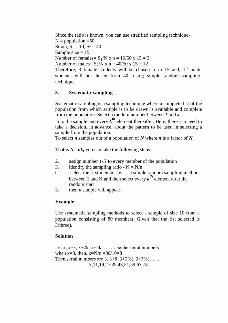
Since the ratio is known, you can use stratified sampling technique-

N = population =50

Strata; S1 = 10, S2 = 40

Sample size = 15

Number of females= S1/N x n = 10/50 x 15 = 3

Number of males= S2/N x n = 40/50 x 15 = 12

Therefore, 3 female students will be chosen form 15 and, 12 male

students will be chosen from 40- using simple random sampling

technique.

3. Systematic sampling

Systematic sampling is a sampling technique where a complete list of the population from which sample is to be drawn is available and complete from the population. Select a random number between 1 and k

in to the sample and every kth

element thereafter. Here, there is a need to take a decision, in advance, about the pattern to be used in selecting a sample from the population.

To select n samples out of a population of N where n is a factor of N.

That is N= nk, you can take the following steps:

2. assign number 1-N to every member of the population 3. identify the sampling ratio - K = N/n c. select the first member by a simple random sampling method,

between 1 and K and then select every kth

element after the random start

3. then n sample will appear.

Example

Use systematic sampling methods to select a sample of size 10 from a

population consisting of 80 members. Given that the fist selected is

3(three).

Solution

Let x, x+k, x+2k, x+3k, ……. be the serial numbers

when x=3, then, k=N/n =80/10=8

Then serial numbers are 3, 3+8, 3+2(8), 3+3(8)……

=3,11,19,27,35,43,51,59,67,78.

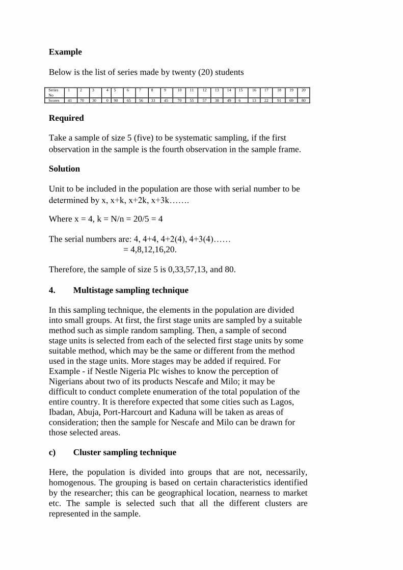
Example

Below is the list of series made by twenty (20) students

Series 1 2 3 4 5 6 7 8 9 10 11 12 13 14 15 16 17 18 19 20

No

Scores 41 70 30 0 90 65 56 33 45 70 55 57 38 49 6 13 22 91 69 80

Required

Take a sample of size 5 (five) to be systematic sampling, if the first

observation in the sample is the fourth observation in the sample frame.

Solution

Unit to be included in the population are those with serial number to be

determined by x, x+k, x+2k, x+3k…….

Where x = 4, k = N/n = 20/5 = 4

The serial numbers are: 4, 4+4, 4+2(4), 4+3(4)……

= 4,8,12,16,20.

Therefore, the sample of size 5 is 0,33,57,13, and 80.

4. Multistage sampling technique

In this sampling technique, the elements in the population are divided

into small groups. At first, the first stage units are sampled by a suitable

method such as simple random sampling. Then, a sample of second

stage units is selected from each of the selected first stage units by some

suitable method, which may be the same or different from the method

used in the stage units. More stages may be added if required. For

Example - if Nestle Nigeria Plc wishes to know the perception of

Nigerians about two of its products Nescafe and Milo; it may be

difficult to conduct complete enumeration of the total population of the

entire country. It is therefore expected that some cities such as Lagos,

Ibadan, Abuja, Port-Harcourt and Kaduna will be taken as areas of

consideration; then the sample for Nescafe and Milo can be drawn for

those selected areas.

c) Cluster sampling technique

Here, the population is divided into groups that are not, necessarily,

homogenous. The grouping is based on certain characteristics identified

by the researcher; this can be geographical location, nearness to market

etc. The sample is selected such that all the different clusters are

represented in the sample.

3.1.2 Non-Probabilistic Sampling

These are sampling techniques that are not probabilistic in estimating and

interpreting the representative sample from the population. Non-

probabilistic sampling includes the following.

2. Judgement sampling or purposive sampling 3. Quota sampling technique 4. Chunk /convenience sampling 5. Volunteer sampling technique

= Judgement sampling technique

This is a sampling method in which the choice sample is dependent,

exclusively, on the discretion of the researcher. The researcher decides

on what items to be included in the sample, based on what he thinks is

most useful or needed.

3. Quota sampling technique

This is a form of judgment sampling. In a quota sampling, the population

is broken down into groups based on some established characteristics

related to the population such as income groups, age, sex, race,

geographical location, etc.; each interviewer is then required to interview

a certain number of persons which constitute the quotas. The selection of

sample items depends on personal judgement.

c) Chunk or convenience sampling technique

This is a sampling method carried out with convenience. For example, if

a researcher wishes to carry out investigation on the effect of motivation

on performance in water producing company; if he/she decides to use a

company close to his/her house, he/she has used convenience method of

sampling- irrespective of the method of selection, as the company chosen

may not be a true representative of the population.

d. Volunteer sampling technique

Here, sampling is done without any compulsion.

SELF-ASSESSMENT EXERCISE

How will you use systematic sampling to select a sample of size 15 from

a population consisting 90 members?

4.0 CONCLUSION

This unit has enabled you to understand what you should do whenever

you have chosen a research topic. You will discover that the method of

sampling is paramount to the population size you have prescribed for

your research work. It equally affects your experimental design.

5.0 SUMMARY

In this unit, you learnt the following:

c) types of sampling techniques. You learnt about simple random

sampling techniques- which means that every member of the

population has to be included in the sample, and you were exposed

to the method you can use to achieve this. You also learnt about

quota sampling technique which is non-probabilistic. It is,

especially, convenient for a wide spread geographical population.

d) the importance of sampling techniques.

6.0 TUTOR-MARKED ASSIGNMENT State the advantages of samples over total enumeration. List and explain the steps you would take in sampling survey.


Adamu, I. M. (2006). Understanding Basic Statistics. Nile Ventures.

Babatunde, L. & Elegbede, W. (2005). Business Statistics: Concepts

and Application. Life and Ministry Publications.

Kazmier, L. (1972). Schaum’s Outline of Theory and Problems of

Statistics. (SI Metric Edition). Singapore: McGraw Hill.

Lind, D., Marchal, W. & Wathen, S. (2010). Statistical Techniques in

Business and Economics. (4th ed.). McGraw-Hill.

course code: bfn728 course title: quantitative techniques ... · this course, bfn 728: quantitative...

Documents