cp based sequence mining on the cloud using spark

Available at:http://hdl.handle.net/2078.1/thesis:10532

[Downloaded 2017/11/23 at 11:29:01 ]

"CP Based Sequence Mining on the Cloud Using Spark"

de Vogelaere, Cyril

AbstractSequential pattern mining (SPM) is a challenging problem concerned withdiscovering frequent pattern in a given sequence dataset. Due to it's broad rangeof applications and it's relative complexity, it has been widely studied in the lasttwo decades and a wide variety of efficient approaches have been developed,notably CP-based approaches which combine both great efficiency and flexibilitythrough the addition of constraints. With the advent of Big-data allowing large-scale data processing through parallel computation, most specialised approachesevolved further and displayed a qualitative step forward in efficiency. However,CP-based approaches have yet to be adapted to support parallel computationsas parallel CP frameworks have yet to be developed. In this paper we thuspropose a novel parallel sequential pattern mining approach based on constraintprogramming modules, and designed to efficiently tackle large-scale data miningproblems through parallel computations in a scalable...

Document type : Mémoire (Thesis)

Référence bibliographique

de Vogelaere, Cyril. CP Based Sequence Mining on the Cloud Using Spark. Ecole polytechniquede Louvain, Université catholique de Louvain, 2017. Prom. : Schaus, Pierre.

CP Based Sequence Mining on the Cloud Using Spark

Dissertation presented by

Cyril DE VOGELAERE

for obtaining the Master’s degree in

Computer Science

Supervisor(s)

Pierre SCHAUS

Reader(s)

John AOGA, Guillaume DERVAL , Nijssen SIEGFRIED , Roberto D’AMBROSIO

Academic year 2016-2017

Contents

List of Figures 3

List of Tables 3

1 Introduction 5

2 Sequential Pattern Mining 72.1 Sequential Pattern Mining Background . . . . . . . . . . . . . . . . . . . . . . . . 7

2.1.1 Definitions and Concepts . . . . . . . . . . . . . . . . . . . . . . . . . . . 72.1.2 Existing specialised approaches . . . . . . . . . . . . . . . . . . . . . . . . 8

2.1.2.1 Apriori . . . . . . . . . . . . . . . . . . . . . . . . . . . . . . . . 82.1.2.2 GSP . . . . . . . . . . . . . . . . . . . . . . . . . . . . . . . . . . 92.1.2.3 PrefixSpan . . . . . . . . . . . . . . . . . . . . . . . . . . . . . . 102.1.2.4 cSPADE . . . . . . . . . . . . . . . . . . . . . . . . . . . . . . . 10

2.1.3 Existing CP Based approaches . . . . . . . . . . . . . . . . . . . . . . . . 122.1.3.1 CPSM . . . . . . . . . . . . . . . . . . . . . . . . . . . . . . . . . 122.1.3.2 PP . . . . . . . . . . . . . . . . . . . . . . . . . . . . . . . . . . 132.1.3.3 Gap-Seq . . . . . . . . . . . . . . . . . . . . . . . . . . . . . . . 132.1.3.4 PPIC . . . . . . . . . . . . . . . . . . . . . . . . . . . . . . . . . 14

2.2 Parallelisation . . . . . . . . . . . . . . . . . . . . . . . . . . . . . . . . . . . . . . 152.2.1 The Benefits of Parallelisation . . . . . . . . . . . . . . . . . . . . . . . . 152.2.2 Tool Selection . . . . . . . . . . . . . . . . . . . . . . . . . . . . . . . . . . 15

2.2.2.1 Hadoop . . . . . . . . . . . . . . . . . . . . . . . . . . . . . . . . 152.2.2.2 Spark . . . . . . . . . . . . . . . . . . . . . . . . . . . . . . . . . 172.2.2.3 Final Choice . . . . . . . . . . . . . . . . . . . . . . . . . . . . . 17

3 Implementation of a Scalable CP Based Algorithm 193.1 Spark’s original implementation . . . . . . . . . . . . . . . . . . . . . . . . . . . . 193.2 A First Scalable CP Based Implementation . . . . . . . . . . . . . . . . . . . . . 21

3.2.1 Improvements Pathways . . . . . . . . . . . . . . . . . . . . . . . . . . . . 213.3 Adding new functionalities . . . . . . . . . . . . . . . . . . . . . . . . . . . . . . . 22

3.3.1 Quicker - Start . . . . . . . . . . . . . . . . . . . . . . . . . . . . . . . . . 233.3.2 Cleaning Sequence before the Local Execution . . . . . . . . . . . . . . . 23

3.4 Improving the Switch to a CP Local Execution . . . . . . . . . . . . . . . . . . . 233.4.1 Automatic Choice of the Local Execution Algorithm . . . . . . . . . . . . 233.4.2 Generalised Pre-Processing Before the Local Execution . . . . . . . . . . 24

3.5 Improving the Scalable Execution . . . . . . . . . . . . . . . . . . . . . . . . . . . 243.5.1 Position Lists . . . . . . . . . . . . . . . . . . . . . . . . . . . . . . . . . . 243.5.2 Specialising the Scalable Execution . . . . . . . . . . . . . . . . . . . . . . 253.5.3 Priority Scheduling for Sub-Problems . . . . . . . . . . . . . . . . . . . . 26

3.5.3.1 Analysing sub-problem creation . . . . . . . . . . . . . . . . . . 263.5.3.2 Sort sub-problem on the reducer . . . . . . . . . . . . . . . . . . 263.5.3.3 Sort sub-problem on the mapper . . . . . . . . . . . . . . . . . . 27

3.6 CP Based Local Execution for Sequence of Sets of Symbols . . . . . . . . . . . . 273.6.1 Pushing PPIC’s Ideas Further . . . . . . . . . . . . . . . . . . . . . . . . . 273.6.2 Adding Partial Projections to PPIC . . . . . . . . . . . . . . . . . . . . . 28

3.7 Final implementation . . . . . . . . . . . . . . . . . . . . . . . . . . . . . . . . . . 283.7.1 Reaching Greater Performances . . . . . . . . . . . . . . . . . . . . . . . . 293.7.2 A New Functionality . . . . . . . . . . . . . . . . . . . . . . . . . . . . . . 30

1

4 Performances 324.1 Datasets . . . . . . . . . . . . . . . . . . . . . . . . . . . . . . . . . . . . . . . . . 324.2 Number of Partitions . . . . . . . . . . . . . . . . . . . . . . . . . . . . . . . . . . 324.3 Performance Testing Procedure . . . . . . . . . . . . . . . . . . . . . . . . . . . . 33

4.3.1 Distribution Choice & Cluster Architecture . . . . . . . . . . . . . . . . . 334.3.2 Program Parameters . . . . . . . . . . . . . . . . . . . . . . . . . . . . . . 334.3.3 Measurement Span . . . . . . . . . . . . . . . . . . . . . . . . . . . . . . . 34

4.4 Testing the Implementations . . . . . . . . . . . . . . . . . . . . . . . . . . . . . 344.4.1 Comparing Spark and PPIC’s original implementations . . . . . . . . . . 344.4.2 Performances of our First CP Based Implementation . . . . . . . . . . . . 344.4.3 Performances of Quicker-Start . . . . . . . . . . . . . . . . . . . . . . . . 374.4.4 Performances of Adding Pre-processing Before PPIC’s Local Execution . 384.4.5 Performances with Automatic choice of Local Execution . . . . . . . . . . 404.4.6 Performances of Adding Pre-processing Before Any Local Execution . . . 414.4.7 Performances with Position lists . . . . . . . . . . . . . . . . . . . . . . . 424.4.8 Performances with Specialised scalable execution . . . . . . . . . . . . . . 434.4.9 Performances of Using Priority Scheduling for the Local Execution . . . . 44

4.4.9.1 Performances of Sorting Sub-Problems on the Reducer . . . . . 444.4.9.2 Performances of Sorting Sub-Problems on the Mapper . . . . . . 45

4.4.10 Performances of using a Map Based Sequence Database Structure . . . . 464.4.11 Performances PPIC with Partial Projection . . . . . . . . . . . . . . . . . 474.4.12 Performances of our final implementation . . . . . . . . . . . . . . . . . . 47

4.5 Scalability Tests . . . . . . . . . . . . . . . . . . . . . . . . . . . . . . . . . . . . 504.5.1 Scalability of the Original Implementation of Spark . . . . . . . . . . . . . 504.5.2 Scalability of our final implementation . . . . . . . . . . . . . . . . . . . . 50

5 Conclusion 53

6 References 54

7 Annexes 567.1 Glossary: . . . . . . . . . . . . . . . . . . . . . . . . . . . . . . . . . . . . . . . . 567.2 Additional example images . . . . . . . . . . . . . . . . . . . . . . . . . . . . . . 567.3 Additional Performance Comparisons: . . . . . . . . . . . . . . . . . . . . . . . . 567.4 Algorithms: . . . . . . . . . . . . . . . . . . . . . . . . . . . . . . . . . . . . . . . 61

8 Acknowledgment 79

2

List of Figures

1 PrefixSpan example . . . . . . . . . . . . . . . . . . . . . . . . . . . . . . . . . . 112 cSPADE database representation . . . . . . . . . . . . . . . . . . . . . . . . . . . 123 cSPADE’s ID-lists . . . . . . . . . . . . . . . . . . . . . . . . . . . . . . . . . . . 124 An example of PPIC’s execution . . . . . . . . . . . . . . . . . . . . . . . . . . . 165 Performance comparison of Hadoop and Spark . . . . . . . . . . . . . . . . . . . 176 An example of Spark’s execution . . . . . . . . . . . . . . . . . . . . . . . . . . . 207 Spark’s mapReduce . . . . . . . . . . . . . . . . . . . . . . . . . . . . . . . . . . . 268 The simple architecture used during the majority of our tests . . . . . . . . . . . 349 Original performances of PPIC and Spark . . . . . . . . . . . . . . . . . . . . . . 3510 A first implementation that makes PPIC scalable . . . . . . . . . . . . . . . . . . 3611 The performance impact of not recalculating frequent items . . . . . . . . . . . . 3812 The performance impact of Database Pre-processing Before PPIC’s Execution . . 3913 Automatic detection of item-sets type in dataset . . . . . . . . . . . . . . . . . . 4014 E�ciency gains of cleaning the sequence database before any local execution . . 4115 Performance gain of first/last position lists . . . . . . . . . . . . . . . . . . . . . 4216 Performance improvement of specialising spark’s scalable stage. . . . . . . . . . . 4317 Naive priority scheduling . . . . . . . . . . . . . . . . . . . . . . . . . . . . . . . . 4418 Performance improvement of sorting sub-problems during map stage. . . . . . . . 4519 Map based - multi_item algorithm . . . . . . . . . . . . . . . . . . . . . . . . . . 4620 PPIC with partial starts . . . . . . . . . . . . . . . . . . . . . . . . . . . . . . . . 4821 Performance of our final implementation . . . . . . . . . . . . . . . . . . . . . . . 4922 Scalability performances of the original implementation . . . . . . . . . . . . . . 5123 Scalability performances of our final implementation . . . . . . . . . . . . . . . . 5224 Example of an S-matrix for PrefixSpan bi-level projection . . . . . . . . . . . . . 5625 PPIC’s performances VS other specialized algorithm . . . . . . . . . . . . . . . . 5726 Performance improvement of fixing Spark’s pre-processing . . . . . . . . . . . . . 5827 Performance improvement - soft limit on the number of created sub-problem. . . 5928 PPIC with a map structure . . . . . . . . . . . . . . . . . . . . . . . . . . . . . . 60

List of Tables

1 Dataset features . . . . . . . . . . . . . . . . . . . . . . . . . . . . . . . . . . . . 322 Number of partitions used during performance tests . . . . . . . . . . . . . . . . 33

3

List of Algorithms

1 Final implementation . . . . . . . . . . . . . . . . . . . . . . . . . . . . . . . . . . 312 Prefix Projection Incremental Counting propagator (PPIC) . . . . . . . . . . . . . 613 PPIC Continued . . . . . . . . . . . . . . . . . . . . . . . . . . . . . . . . . . . . . 624 Spark’s original implementation: Pre-Processing . . . . . . . . . . . . . . . . . . . 635 Spark’s original implementation: Scalable execution . . . . . . . . . . . . . . . . . 646 Spark’s original implementation: Local execution . . . . . . . . . . . . . . . . . . . 657 Spark’s original implementation: Project and findPrefixExtension . . . . . . . . . 668 First scalable CP based implementation . . . . . . . . . . . . . . . . . . . . . . . . 679 New functionalities: Scalable execution . . . . . . . . . . . . . . . . . . . . . . . . 6810 Quick - Start: Scalable execution . . . . . . . . . . . . . . . . . . . . . . . . . . . . 6911 Clean database before local execution of PPIC: . . . . . . . . . . . . . . . . . . . . 7012 Automatic Local Execution Selection: . . . . . . . . . . . . . . . . . . . . . . . . . 7113 Clean database before any local execution: . . . . . . . . . . . . . . . . . . . . . . 7214 Positions lists: Project and findPrefixExtension . . . . . . . . . . . . . . . . . . . . 7315 Specialised Execution: Pre-Processing . . . . . . . . . . . . . . . . . . . . . . . . . 7416 Sorting sub-problems on the reducer: . . . . . . . . . . . . . . . . . . . . . . . . . 7517 Sorting sub-problems on the mapper: . . . . . . . . . . . . . . . . . . . . . . . . . 7618 PPIC with a Map based Structure (partial pruning): . . . . . . . . . . . . . . . . . 7719 PPIC with partial projections: . . . . . . . . . . . . . . . . . . . . . . . . . . . . . 78

4

Abstract

Sequential pattern mining (SPM) is a challenging problem concerned with discoveringfrequent pattern in a given sequence dataset. Due to it’s broad range of applications and it’srelative complexity, it has been widely studied in the last two decades and a wide variety ofe�cient approaches have been developed, notably CP-based approaches which combine bothgreat e�ciency and flexibility through the addition of constraints.

With the advent of Big-data allowing large-scale data processing through parallel compu-tation, most specialised approaches evolved further and displayed a qualitative step forwardin e�ciency. However, CP-based approaches have yet to be adapted to support parallelcomputations as parallel CP frameworks have yet to be developed.

In this paper we thus propose a novel parallel sequential pattern mining approach basedon constraint programming modules, and designed to e�ciently tackle large-scale data miningproblems through parallel computations in a scalable environment.

In this endeavour, we use the recently designed CP-based algorithm PPIC, which outper-form both other CP-based and specialised approaches by using ideas from both data miningand CP on a generic constraint solver, to locally solve sub-problems generated through ageneric, map-reduce based, scalable PrefixSpan algorithm implemented using Spark.

We then show through detailed experimentation on popular datasets that, through thisnovel implementation, great performances can be obtained in a scalable architecture withoutlosing much flexibility on the supported constraints.

1 Introduction

Sequential pattern mining (SPM) is a widely studied problem concerned with discovering frequentsub-sequences in a sequence database. The problem of SPM is to find all patterns in a sequencedatabase with respect to the frequency constraint. The frequency is the number of number ofoccurrences of a pattern in the database. This problem has broad applications, including butnot limited to: Analysis of customer purchase patterns, web-log mining, medical research, DNAsequencing, text-mining, human mobility mining, ... [1].

First introduced by Agrawal and Srikant in 1995 [2], sequential pattern mining problems havesince been widely studied for more e�cient way to find their combinatorially explosive numberof possible subsequence patterns. Many techniques such as Apriori [2], GSP [3], cSPADE [4],and PrefixSpan [5] have thus been proposed to e�ciently solve this problem.

Recently, constraint programming (CP) has been proposed as a framework for sequentialpattern mining problems to solve the lack of flexibility and modularity of the previously citedapproaches. Thus, various e�cient CP-based algorithm such as CPSM [6], or Gap-Seq [7] wheredeveloped. The main benefit of those algorithms is their modularity, since their implementationsallow the addition of multiple constraints to restrict the search space of the problem, and moree�ciently work toward specific solutions. Those constraints encompassing a wide range ofpossibilities such as imposing frequency restrictions, imposing restrictions on the pattern length,ensuring the respect of regular expressions, ... .

However, this increased flexibility can come with a performance cost. Many of the developedalgorithm staying uncompetitive in comparison to state-of-the-art specialised methods. However,many recently made improvements, notably by Kemmar et al [7, 8], which had further extendedthis work by introducing one constraint (module) for both the pseudo-projection and the fre-quency pruning, and allowed CP based sequence mining algorithms to become competitive withstate-of-the-art techniques such as Zaki’s cSPADE [9].

A recent paper [10] went even further by designing a CP based implementation that greatlyout-performs state-of-the-art implementations. This PrefixSpan based algorithm called PPIC,

5

designed to find patterns on sequences of individual symbols and implemented on the open sourceCP-solver OscaR [11], achieved those improved performances by combining ideas from patternmining and constraint programming.

More specifically, this new algorithm improves the e�ciency of computing prefix-projecteddatabases (the usual bottleneck of PrefixSpan based techniques) by using ideas from the LAPIN-SPAM algorithm [12]. This algorithm also improves the time needed to restore projected databasewhen using a depth-first search (DFS) approach through the use of trailing which avoid unneces-sary copies of the data.

However, the previously mentioned implementations were not ready for the recent advent ofBig Data, as they were not adapted for large-scale data processing. Those implementation thusneeded to evolve and support parallel computations, so that they could be executed in scalable’big-data’ environments and display further improved performances.

While non-CP algorithms were quickly adapted to those new environments with the intro-duction of a scalable implementation based on PrefixSpan [13] and cSPADE [14], CP-basedapproaches have yet to be adapted to support parallel computations.

Our objective in this paper is thus to adapt the recently designed PPIC algorithm to e�cientlysupport parallel computations in a scalable architecture. Additionally, we took extra care to trykeeping the inherent flexibility of CP-based implementation without sacrificing performances.

The reminder of this paper is thus organized as follows: In Section 2 we present the necessarybackground knowledge allowing one to understand SPM problems. Section 3 then explains andmotive the di�erent parallel implementation created during this master thesis, including thefinal implementation which combine their strength. Finally Section 4 present the performancemeasured on each implementations, as well as the scalable performances of both the originalimplementation and our final implementation.

6

2 Sequential Pattern Mining

Sequence pattern mining (SPM) is a widely studied problem focusing on discovering sub-sequencesin a dataset of given sequences. Each (sub) sequence being an ordered list of symbols, or setsof symbols. SPM has applications ranging from web log mining and text mining, to biologicalsequence analysis.

2.1 Sequential Pattern Mining Background

2.1.1 Definitions and Concepts

Definition 1. Symbol, Item and Item-sets: A symbol (si) is an element of a sequence,symbols can be repeated in sequences but, in a given database, a symbol will keep the samemeaning. Symbols can be grouped into sets of symbols.An item (i) is the integer representation of a symbol. While symbols could technically be anythingfrom an Object to a primitive type, items are integer representation of those symbols allowingshorter representation of the database. Similarly, items can be grouped in sets, we refer to sets ofitems as Item-sets. Thus given S = {s1, ... , sM } a set of M symbols where there is no ambiguity,the set of items representing these symbols is given by I œ {1, ..., N}.In the remainder of this paper, we refer to elements of sequence as symbols unless a representationas Item is necessary for the algorithm/concept concerned.

Definition 2. Sequence: A sequence seq = {S1, S2, ..., SM } is an ordered list of sets of symbolsSj , j œ [1, M ]. The sequence of length N (N = qM

j=1 |Sj|) is called an N-length sequence. Forexample: Èa(ab)Í and ÈabcÍ are both 3-length sequences.

In the remained of this paper, we distinguish between two types of sequences. If a sequenceof length N specifically contains M=N sets of symbols, we refer to it as a sequence of symbols(SoS). Otherwise, if a sequence contains a non-specified number of item M (1 Æ M Æ N), werefer to it as a sequence of sets of symbols (SoSS).

Example 1. Type of Sequences

• È(A B)D E(C A)Í is a sequence of sets of symbols (SoSS), where parenthesis act as delimitersbetween symbol sets. We are have two symbol sets (A B) and (C A) containing two symbolseach for a total sequence length of 4.

• ÈA B C AÍ is a sequence of symbols (SoS) of length 4 containing three di�erent symbols.Symbol A being repeated multiple times in the sequence. Similarly È(A)(B)(C)(A)Í is also aSoS despite the presence of separators, since each symbol set contains at most one element.

Definition 3. Sub-Sequence (∞) / Super-Sequence: A sequence – = {–1, –2, ..., –m} is asubsequence of seq = {S1, S2, ..., Sn} and seq is a super-sequence of – if and only if: m Æ n andthere exist a one-to-one order-preserving function f that maps sets in – to sets in seq such that’i œ [1, M ], –i µ f(–i) and ’i, j with j > i, f(–i) occurs before f(–j) in seq.

Definition 4. Sequence database: A sequence database is a non-ordered collection of set oftuples (sid, seq). Where ’sid’ is a sequence identifier and ’seq’ a sequence. If a sequence databasecan only contains sequences of symbols, we shall denote it as SDB in the remained of this paper.In any other case we shall refer to the database by using the acronym SSDB.Any algorithm mining sequential pattern for an SSDB should find the same solutions for SDBdatasets as an SDB only algorithm. SDB specialised algorithms may never be used on SSDB.

Example 2. Type of Sequences Database

• (ÈA B C AÍ, ÈD E C BÍ) is an SDB, since it contains only sequences of symbols.

7

• (È(A)(B)Í, È(D)(E)(C)(B)Í) is also an SDB, since it similarly only contains sequences ofsymbols, the maximal Symbol Set size being one.

• (È(A)(B)(C A)Í, È(D)(E)(C)(B)Í) is an SSDB, since it contains at least one sequence ofsets of symbols, the first sequence of the database which contains (C A), a symbol set withmultiple symbols.

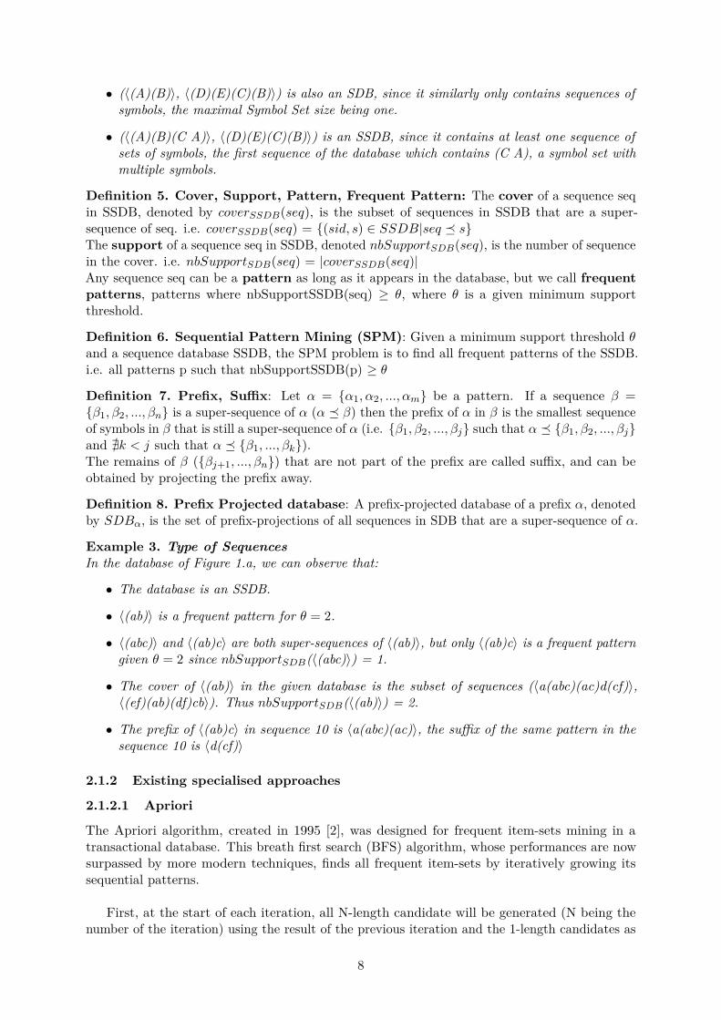
Definition 5. Cover, Support, Pattern, Frequent Pattern: The cover of a sequence seqin SSDB, denoted by coverSSDB(seq), is the subset of sequences in SSDB that are a super-sequence of seq. i.e. coverSSDB(seq) = {(sid, s) œ SSDB|seq ∞ s}The support of a sequence seq in SSDB, denoted nbSupportSDB(seq), is the number of sequencein the cover. i.e. nbSupportSDB(seq) = |coverSSDB(seq)|Any sequence seq can be a pattern as long as it appears in the database, but we call frequentpatterns, patterns where nbSupportSSDB(seq) Ø ◊, where ◊ is a given minimum supportthreshold.

Definition 6. Sequential Pattern Mining (SPM): Given a minimum support threshold ◊and a sequence database SSDB, the SPM problem is to find all frequent patterns of the SSDB.i.e. all patterns p such that nbSupportSSDB(p) Ø ◊

Definition 7. Prefix, Su�x: Let – = {–1, –2, ..., –m} be a pattern. If a sequence — ={—1, —2, ..., —n} is a super-sequence of – (– ∞ —) then the prefix of – in — is the smallest sequenceof symbols in — that is still a super-sequence of – (i.e. {—1, —2, ..., —j} such that – ∞ {—1, —2, ..., —j}and @k < j such that – ∞ {—1, ..., —k}).The remains of — ({—j+1, ..., —n}) that are not part of the prefix are called su�x, and can beobtained by projecting the prefix away.

Definition 8. Prefix Projected database: A prefix-projected database of a prefix –, denotedby SDB–, is the set of prefix-projections of all sequences in SDB that are a super-sequence of –.

Example 3. Type of Sequences

In the database of Figure 1.a, we can observe that:

• The database is an SSDB.

• È(ab)Í is a frequent pattern for ◊ = 2.

• È(abc)Í and È(ab)cÍ are both super-sequences of È(ab)Í, but only È(ab)cÍ is a frequent patterngiven ◊ = 2 since nbSupportSDB(È(abc)Í) = 1.

• The cover of È(ab)Í in the given database is the subset of sequences (Èa(abc)(ac)d(cf)Í,È(ef)(ab)(df)cbÍ). Thus nbSupportSDB(È(ab)Í) = 2.

• The prefix of È(ab)cÍ in sequence 10 is Èa(abc)(ac)Í, the su�x of the same pattern in thesequence 10 is Èd(cf)Í

2.1.2 Existing specialised approaches

2.1.2.1 Apriori

The Apriori algorithm, created in 1995 [2], was designed for frequent item-sets mining in atransactional database. This breath first search (BFS) algorithm, whose performances are nowsurpassed by more modern techniques, finds all frequent item-sets by iteratively growing itssequential patterns.

First, at the start of each iteration, all N-length candidate will be generated (N being thenumber of the iteration) using the result of the previous iteration and the 1-length candidates as

8

basis. The support of those candidates will then be checked with the databases and un-frequentpattern will be deleted. Finally, frequent N-length patterns will be sent onto the next iteration,until none can be grown.

While historically relevant, this algorithm was ine�ciently generating all possible N-lengthcandidates using the N-1-length candidates as basis. Among those a large amount of candidatewouldn’t be frequent, and would thus waste huge amount of memory and CPU time being stockedand uselessly verified across the database.

One of its good points however, lies in its ability to be used to detect association rules (Example:When A is present, B has 75% chance of being also present), which can give indications aboutthe general trends in the database and allow human operators to get a general understanding ofthe inputted dataset.

2.1.2.2 GSP

The Generalised Sequential Pattern (GSP) algorithm [3] was based on the Apriori algorithmbut redesigned for sequential pattern mining instead of frequent item-set mining. One of thegood points of this new algorithm lied in the possibility to add time constraints that specified aminimum and/or maximum time period between adjacent elements in a pattern.

As Apriori, the algorithm start by detecting frequent 1-length pattern, it then proceedswith generating all 2-length patterns from there. However, since order now matters as itemsthat should be grouped together can come from multiple transactions, there is now a lot morecandidates to create.

More specifically, given two items A and B, the generated candidate would be AB, BA and(AB). (AB) being the representation of those two items occurring in the same transactionaltime frame. Those candidates will then be projected on the database, and their support will becounted. All candidates having a lesser amount of support than the threshold ◊ will then becleaned.

The algorithm should then generate further candidates, but unlike Apriori, the method hasbeen complexified to become far more e�cient. Instead of growing sequential patterns by addingall 1-length patterns to each of their end and creating a tremendous amount of unsupportedpatterns, we create those candidates more e�ciently.

First, for each sequential patterns of N-length found in the previous iterations, we detect itsfirst and last N-1 item, thus creating two sub-sequential patterns by omitting an element eitherat the end or start. We will then create N+1-length candidates by composing sequential patternswith similar end and start sub-sequential pattern.

For example, given the sequential patterns AA, (AB), AB and BA, we would be able togenerate the following candidates: A(AB), (AB)A, B(AB), (AB)B, ABA, BAB, AAB, BAA.Those candidates should then be pruned to remove impossible combinations found in previousiterations. In the case of our example, since BB was not retained as a 2-length sequential patterndue to being un-frequent, we can delete all candidate sequential patterns containing BB, as theysimilarly cannot be present.We are thus left with: A(AB), (AB)A, ABA, AAB, BAA

Finally, we count the number of support for each candidates having passed the pruning phase,and remove unsupported sequential patterns. Another iteration of generating candidates, pruning

9

and count support will then start, until no supported sequential patterns is found at the end ofan iteration, or no candidates can be generated.

If after counting the support of each candidate we detect that only ABA and BAA aresupported, the next iteration would only create the candidate ABAA. Since it would be ouronly 4-length pattern, no 5-length pattern will be generated and the execution will stop havingdetermined that all solutions were found.

As you may expect, this new method to generate candidates allowed GSP to surpass Apriori’se�ciency by a wide margin. Since the algorithm additionally supported a wide range of newconstraints allowing reduction of the search space, and was so e�cient, it became a referencealgorithm in frequent pattern mining.

2.1.2.3 PrefixSpan

The PrefixSpan approach [5] relies on pattern growth. As you may see in our simple exampledisplayed in Figure 1, the idea of this algorithm is to find the complete set of patterns throughiteratively growing prefixes by projecting them on the database, and finding extensions.

The main selling point of the algorithm lies in its ability to quickly generate candidateextensions, projecting prefixes on the database significantly reducing the time needed to findprefixes extensions, as only the su�xes need to be searched for those extensions to be found.Another selling point lies in its scalability, as this method is easily implementable under aMap-Combine-Reduce programming scheme.

However, this method also has disadvantages, mainly in the fact that projecting databases isa time expensive process. Making building those projected databases the e�ciency bottle-neckof PrefixSpan.

Fortunately, techniques exists to break past this bottle-neck and mitigate its e�ects. Tech-niques among which we should mention the ’Bi-level projection’ technique, which consists increating a triangular matrix (S-matrix [24]) registering the number of supports for all 2-lengthsequences that can be assembled from 1-length prefixes. A quick scan of the S-matrix thenallows the detection of all supported 2-length prefixes, prefixes which can then be extended againthrough applying the same technique on their projected database. Thus allowing a reduction ofthe number of necessary prefix projections during the execution of the algorithm, since only halfof the prefixes will need to be projected.

A second technique we should mention is the ’Pseudo-Projection’ technique which is basedon keeping and maintaining a start index for each sequence. This start-index registering thelowest position at which the last projected prefix was supported, thus allowing quicker projectionof extending prefixes by avoiding to re-project previous prefix elements.

2.1.2.4 cSPADE

The cSPADE algorithm [9] uses combinatorial properties to divide the original sequence patternmining problem in smaller sub-problems that can be solved independently using simple id-listjoin operations. This algorithm is thus parallelisable, furthermore, the parallelisation has a linearscalability with respect to the size of the inputted database.

cSPADE’s first step is to compute all 1-length sequential patterns using a simple databasescan. Then, we generate all 2-length sequential patterns and count the number of supporting

10

(a) Original database of our SPM example

(b) Prefix projected databases relative to 1-length sequential patterns &final list of sequential patterns eventually extended from those 1-length prefixes

Please take note that underscores in the projected databases represent itemSet’s items that havebeen ’consumed’ by the projection. Since we consider that itemSets are sorted in PrefixSpan,smaller item are ’consumed’ when projecting larger item on itemSets. For example, projecting

pattern ÈbÍ on sequence 10 will also ’consume’ item a in the first itemSet (abc).

Figure 1: PrefixSpan example

sequences for each pair of items in a bi-dimensional matrix. Counting the number of supportingsequence being realised through another database scan by first transforming the original verticalrepresentation of the database into an horizontal representation (see Figure 2).

Subsequent N-length sequence patterns can then be formed by joining (N+1)-length patternsusing their id-lists (list of positions in sequences for each item, see Figure 3). The support ofeach item can also be easily calculated from ID-list, as we just need to count the number ofdi�erent sequences in which it appears.

It is also important to note that this method of joining ID-lists is only e�cient from 3-lengthpatterns onward, as ID-lists for length 1 and 2 patterns can be extremely large and potentiallywouldn’t fit in memory.

Of course, at the end of each round, un-frequent sequential pattern should be cleaned asto guarantee only frequent patterns will be extended. This algorithm can be executed usingeither breadth first or depth first search, and ends its execution once no patterns can be furtherextended.

11

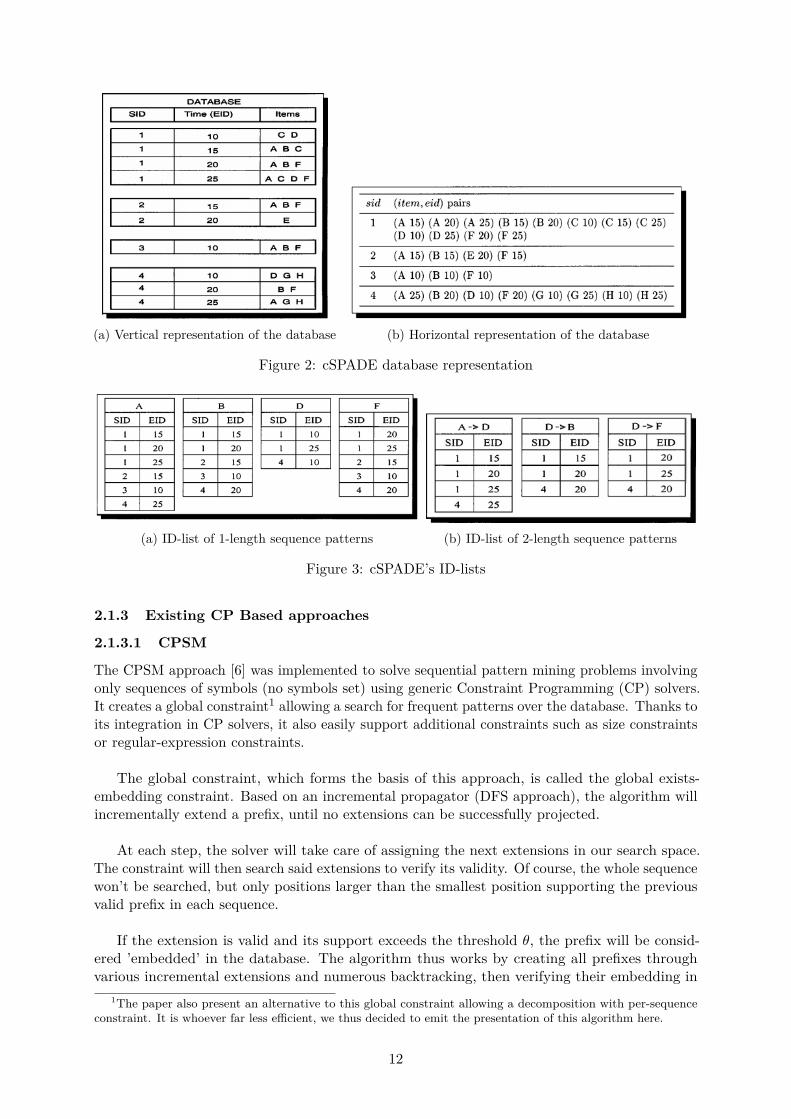
(a) Vertical representation of the database (b) Horizontal representation of the database

Figure 2: cSPADE database representation

(a) ID-list of 1-length sequence patterns (b) ID-list of 2-length sequence patterns

Figure 3: cSPADE’s ID-lists

2.1.3 Existing CP Based approaches

2.1.3.1 CPSM

The CPSM approach [6] was implemented to solve sequential pattern mining problems involvingonly sequences of symbols (no symbols set) using generic Constraint Programming (CP) solvers.It creates a global constraint1 allowing a search for frequent patterns over the database. Thanks toits integration in CP solvers, it also easily support additional constraints such as size constraintsor regular-expression constraints.

The global constraint, which forms the basis of this approach, is called the global exists-embedding constraint. Based on an incremental propagator (DFS approach), the algorithm willincrementally extend a prefix, until no extensions can be successfully projected.

At each step, the solver will take care of assigning the next extensions in our search space.The constraint will then search said extensions to verify its validity. Of course, the whole sequencewon’t be searched, but only positions larger than the smallest position supporting the previousvalid prefix in each sequence.

If the extension is valid and its support exceeds the threshold ◊, the prefix will be consid-ered ’embedded’ in the database. The algorithm thus works by creating all prefixes throughvarious incremental extensions and numerous backtracking, then verifying their embedding in

1The paper also present an alternative to this global constraint allowing a decomposition with per-sequenceconstraint. It is whoever far less e�cient, we thus decided to emit the presentation of this algorithm here.

12

the database.

Since trying all possible extensions at each incremental step would be ine�cient, the algorithmwas also designed to prune the next possible extensions that should be considered by the solver,and only keep extensions that are su�ciently supported in the database. Thus, symbols thatare considered unfrequent won’t be branched over during the execution. This pruning is doneby counting the number of support for each extension during the embedding existence verification.

Although impressive for its modularity, the e�ciency of this algorithm didn’t quite caughtup to specialised non-CP algorithms such as PrefixSpan or cSPADE. It, however, surpassed theire�ciency at searching for specific solutions thanks to its modularity.

2.1.3.2 PP

This second approach based on CPSM proposed a slightly di�erent global constraint by takingideas from prefix-projection [8]. Similarly to its predecessor, this algorithm was designed to solvesequential pattern mining problems involving sequence of symbols (no sets of symbols).

The main idea behind this improved constraint being that we have no need to check sequencesfor extensions support when they did not support sub-sequences of the current prefix.

This new algorithm thus takes notes of the ID of sequences which support the current patternso that its extensions may be projected only on those sequences. The key element of this newfeature being that we keep ID of sequence and not copy of sequences, making it extremelymemory and time e�cient.

During the extensions pruning phase, only supportive sequences will need to be checked in asimilar fashion, as they are the only relevant sequences to find extensions with.

While the rest of this global constraint implementation was very similar to CPSM’s globalconstraint, the prefix projection improvement allowed this new implementation to largely overtakeits predecessors in e�ciency. Making this new algorithm competitive with state-of-the-art non-CPmethod while keeping the improved modularity inherent to CP algorithms.

2.1.3.3 Gap-Seq

This new algorithm introduced a global constraint adding support for time gap constraint [7].This allows, for example, to analyses purchase behaviours and find products usually bought bycustomers at regular time intervals.

Similarly to its predecessors, the algorithm was designed to solve sequential patterns miningproblems involving sequences of symbols, doing so by incrementally extending and verifyingprefixes over multiple pass of a prefix projected database.

The new global constraint, however, allow tighter search spaces where one can specify theminimal/maximal distance allowed between two symbols for them to remain solution.

For this constraint to work e�ciently, additional pruning was added when pruning forextending items, so that extensions which would violate the time gap constraints couldn’t betaken into account.

13

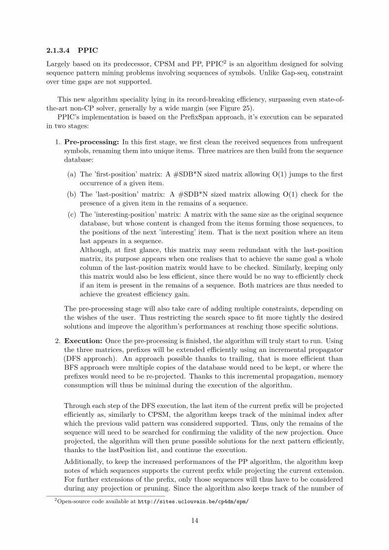
2.1.3.4 PPIC

Largely based on its predecessor, CPSM and PP, PPIC2 is an algorithm designed for solvingsequence pattern mining problems involving sequences of symbols. Unlike Gap-seq, constraintover time gaps are not supported.

This new algorithm speciality lying in its record-breaking e�ciency, surpassing even state-of-the-art non-CP solver, generally by a wide margin (see Figure 25).

PPIC’s implementation is based on the PrefixSpan approach, it’s execution can be separatedin two stages:

1. Pre-processing: In this first stage, we first clean the received sequences from unfrequentsymbols, renaming them into unique items. Three matrices are then build from the sequencedatabase:

(a) The ’first-position’ matrix: A #SDB*N sized matrix allowing O(1) jumps to the firstoccurrence of a given item.

(b) The ’last-position’ matrix: A #SDB*N sized matrix allowing O(1) check for thepresence of a given item in the remains of a sequence.

(c) The ’interesting-position’ matrix: A matrix with the same size as the original sequencedatabase, but whose content is changed from the items forming those sequences, tothe positions of the next ’interesting’ item. That is the next position where an itemlast appears in a sequence.Although, at first glance, this matrix may seem redundant with the last-positionmatrix, its purpose appears when one realises that to achieve the same goal a wholecolumn of the last-position matrix would have to be checked. Similarly, keeping onlythis matrix would also be less e�cient, since there would be no way to e�ciently checkif an item is present in the remains of a sequence. Both matrices are thus needed toachieve the greatest e�ciency gain.

The pre-processing stage will also take care of adding multiple constraints, depending onthe wishes of the user. Thus restricting the search space to fit more tightly the desiredsolutions and improve the algorithm’s performances at reaching those specific solutions.

2. Execution: Once the pre-processing is finished, the algorithm will truly start to run. Usingthe three matrices, prefixes will be extended e�ciently using an incremental propagator(DFS approach). An approach possible thanks to trailing, that is more e�cient thanBFS approach were multiple copies of the database would need to be kept, or where theprefixes would need to be re-projected. Thanks to this incremental propagation, memoryconsumption will thus be minimal during the execution of the algorithm.

Through each step of the DFS execution, the last item of the current prefix will be projectede�ciently as, similarly to CPSM, the algorithm keeps track of the minimal index afterwhich the previous valid pattern was considered supported. Thus, only the remains of thesequence will need to be searched for confirming the validity of the new projection. Onceprojected, the algorithm will then prune possible solutions for the next pattern e�ciently,thanks to the lastPosition list, and continue the execution.Additionally, to keep the increased performances of the PP algorithm, the algorithm keepnotes of which sequences supports the current prefix while projecting the current extension.For further extensions of the prefix, only those sequences will thus have to be consideredduring any projection or pruning. Since the algorithm also keeps track of the number of

2Open-source code available at http://sites.uclouvain.be/cp4dm/spm/

14

http://sites.uclouvain.be/cp4dm/spm/

support for each extension, an improvement was also made to stop searching for projectionsonce that number of supporting sequences have been found during the prefix’s projection.Since the remaining sequences definitely won’t support the item and will remain irrelevantfurther down this branch of the search tree.

Each time a valid solution is found. That is, a solution that satisfy all constraints injectedin the solver. The execution will be momentarily interrupted. The solution will then betranslated back to the symbols corresponding to the recorded items and saved in a result list.

Once the solver determines that no further solution can be found under the specifiedconstraints. The execution will terminate, and all resulting pattern will be returned.

An example of a complete execution of PPIC can be found in Figure 4. The pseudo-code canbe found in Algorithm [2, 3].

Also, there exist a version of PPIC (called PPICt [15])supporting time constraint (GAP,SPAM) and that provides better performances than Gap-Seq and cSPADE.

2.2 Parallelisation

As said previously in the introduction, our goal is to achieve a scalable implementation based onPPIC, a CP algorithm based on the PrefixSpan approach.

2.2.1 The Benefits of Parallelisation

The benefits of achieving such a scalable algorithm are many. First, local algorithms are limitedto the power of the computer they run on, achieving parallelism allows to break that limit andincrease the overall e�ciency by running on multiple computers at once.

Another advantage lies in costs as, with the arrival of cloud technologies, running algorithmson clusters of small machines is gradually becoming cheaper than buying and maintainingsupercomputers.

For both those reasons, and the fact that a large quantity of SPM problems cannot be run onlocal architectures, designing implementations that are both scalable and e�cient has graduallybecome extremely important for the industry.

2.2.2 Tool Selection

Since, fortunately, SPM problems are embarrassingly parallel problem, we had the opportunityto choose from a selection of widely used open-source libraries. We, however, restricted ourselvesto Scala compatible framework, as the CP library supporting PPIC was implemented in thislanguage. Rapidly, we were left to choose from two major options:

1. Hadoop mapreduce

2. Spark

2.2.2.1 Hadoop

Hadoop is an open-source framework that allows large-scale data processing across clustersof machines. Based on a Map-reduce programming model, this framework allows larger scaleiterative computations on humongous quantities of data. At each iteration, the data is read from

15

Input sequences:ÈADBABCAÍ

ÈABCAÍÈADÍ

Number of supporting sequences necessary: 2

Pre-processed sequences:È1421231Í

È1231ÍÈ14Í

indexInSequence:[0, 0, 0]

supportCounter:[3, 2, 2, 2]

firstPosList:[1, 3, 6, 2][1, 2, 3, 0][1, 0, 0, 2]

lastPosList:[7, 5, 6, 2][4, 2, 3, 0][1, 0, 0, 2]

interestingPosList:[2, 5, 5, 5, 6, 7, 0]

[2, 3, 4, 0][2, 0]

Projecting 4:indexInSequence:

[2, 4, 2]sequenceSupported:

[1, 3]itemSupportCounter:

[1, 1, 1, 0]Extensions supported:

[]



[1, 2, 3]itemSupportCounter:


[1, 2, 3, 4]





[]





[]





[1]





[]





[1, 3]





[]





[1]





[]





[1, 3]





[]





[1]





[]





[1]





[]

Figure 4: A simple execution of PPIC’s algorithm.The solution patterns are the projected prefixes

the distributed file system (HDFS), modified through a MapReduce, then stored back on the filesystem.

The advantages of Hadoop thus lies in the simplicity of its usage. Aside from implementingthe Map and Reduce process, Hadoop will take care of scheduling, data repartition and failurerecovery.

Widely used since its initial release on December 10, 2011. Hadoop slowly climbed to becomeone of the big standards in terms of large scale computation. We thus selected it as our potentialscalable framework, discovering shortly after that an e�cient implementation of PrefixSpan onHadoop was already available on the internet.

16

2.2.2.2 Spark

Spark is an open-source engine for large-scale data processing. Mainly reputed for its speed, easeof use, and ability to e�ciently implement sophisticated problems.

Originally developed at UC Berkeley in 2009, Its entire implementation revolves aroundan immutable read-only data structure called the resilient distributed dataset (RDD).Maintained in a fault-tolerant way, those lazily computed RDD, built through deterministiccoarse-grained transformation, have been designed to be e�ciently distributed over a cluster ofmachines, allowing resolution of complex iterative problems in scalable environments.

Furthermore, Spark has been designed to make use of its clusters RAM memory e�ciently,allowing the engine to distance itself from slow HDD memory access. Of course, should the RAMmemory be insu�cient, Spark is perfectly able to run using nothing but the hard-drive.

Spark’s was thus an extremely valid choice from a technical standpoint and, similarly toHadoop, we were surprised to discover an existing implementation of PrefixSpan available inSpark’s machine learning library.

2.2.2.3 Final Choice

As said earlier, both of those libraries already disposed of a scalable PrefixSpan implementation,and both were e�cient and widely recognised framework to achieve parallelism. It was thusa matter of determining whose performances were better, and whether those implementationscould be e�ciently extended through CP technologies.

Fortunately for us, performance comparison had already been done in a widely recognisedscientific paper on Spark’s RDD [16]. Those performances are presented in Figure 5

Figure 5: Performance comparison of Hadoop and Spark

As we can see, performance-wise, Spark vastly outperform Hadoop thanks to its ability touse both memory and disk for its computations. Allowing up to 100x speed-up under the rightcircumstances, as we can see in the logistic regression problem. According to the o�cial website,Spark would also boast a 10x speed-up through on disk computation only, but no performance

17

benchmarks were provided to back that claim.

In terms of extensions through CP technologies, we quickly realised that Hadoop would be farless practical. Although MapReduce can be used to execute the standard PrefixSpan algorithm,and could certainly be modified to introduce CP elements, Spark can support any coarse-grainedtransformation with its RDDs, allowing a more precise implementation where only requiredtransformations would be made, instead of simple sequences of Map-Combine-Reduce.

18

3 Implementation of a Scalable CP Based Algorithm

In this section, we shall present the various implementation we created in an attempt to improveSpark’s original algorithm’s performances. The performance of those implementations, however,will be tested in a later section.

3.1 Spark’s original implementation

Before introducing our various implementation, let us present Spark’s original algorithm. Analgorithm based on the PrefixSpan approach, and can be separated in four stages:

1. Pre-processing: The goal of this stage is to replace each symbol of the sequence databaseby a unique item, to separate item-sets through a zero delimiter, and to clean the databasefrom unfrequent items.For example, the sequence È(ABD)(ABC)AÍ will become 0120123010, assuming only symbolsA, B and C are frequent in the sequence database.

2. Scalable execution: The core of the algorithm. Its execution consists in extendingprefixes through a three sub-stage process, starting from the empty prefix.

(a) First, a large prefix is projected on the database, meaning that only the su�x ofsupporting sequence remain in the resulting database. When there is no prefix toproject, the scalable execution comes to an end and the algorithm goes on to the nextstage.

(b) Then, from the set of supporting sequences, we discover symbols that can extend thecurrent prefix. If no such extension exists, we try the next large prefix.

(c) Finally, for each possible symbol extension, we extend the corresponding prefix.We then determine how long further expanding each extended prefix may take bycalculating the projected database size. Depending on the calculated projected sizeand of the value of a user defined parameter, we then either further extend thisprefix using another iteration of the scalable execution, or store it for use in the localexecution stage.

3. Local execution: The local execution is completely similar in its implementation to thescalable execution. Its only use is in significantly improving the algorithm’s performanceby calculating all extensions from a Prefix locally, instead of doing so while shu�inginformation around the scalable architecture.This stage is only launched once all large prefixes have been extended su�ciently, makingthe projected databases that need to be processed to find future extensions small enough.Depending on the parameters inputted by the user, this stage may be skipped.

4. Post-processing: During the post-processing step, we translate back the unique itemsinto the corresponding symbols they each represented. Then we send back the collectedresults to the user.

During the prefix projection phase of the scalable and local execution, the algorithm will alsodetect which item-sets in the sequence comply with what has already been projected and canstill be extended in some way. Storing such items positions in a ’partial projection’ list.That way, if we are projecting an item-set containing multiple symbols from a prefix, until theend of that item-set, the items projection phases will know where to search possible extensions,preventing the algorithm from having to search the whole sequence.Also, should we be computing on a database of sequence of symbols, no partial start would becreated and kept in memory, since the algorithm would automatically detect that those item-sets

19

cannot be extended.

When the current item-set end, the full remains of the sequence, from the earliest partialposition recorded, will have to be searched for extensions. When extending the first item of thenew item-set, new potential partial projection will be recorded, and the old ones will be discarded.

During the prefix extension phase, the current partial projection will also be used to findextensions of the current item-set quicker. The remainder of the database will also be searched,but only for extension that starts new item-sets.

An example of a fully scalable execution from this algorithm can be found in Figure 6. Apseudo-code can also be found in Algorithm [4, 5, 6, 7].

Input sequences:È(ADB)(ABC)(A)Í

È(ABC)AÍNumber of supporting sequences necessary: 2

Pre-processed sequences:È0120123010Í

È0123010Í

Empty prefix projection:È|0120123010Í

È|0123010ÍPartial starts:

[][]

Extensions found:[01, 02, 03]

Projecting 01:È01|20123010Í

È01|23010ÍPartial starts:

[4][]

Extensions supported:[2, 3, 01]



[][]

Extensions supported:[]



[][]

Extensions supported:[01]



[][]




[5][]

Extensions supported:[3, 01]



[][]


Projecting 012301:È012012301|0Í


[][]




[][]




[][]




[][]




[5][]

Extensions supported:[3, 01]



[][]




[][]




[][]


Figure 6: A simple execution of Spark’s algorithm.The solutions are the projected prefixes (except the empty prefix)

NB: During our first analysis of Spark’s pre-processing stage, we noticed a small ine�ciency inthe cleaning of the database’s sequences. When multiple item-sets were fully cleaned of

20

their item, the algorithm had a tendency of creating sequences of zero delimiters, as thealgorithm still delimited empty item-sets.Although the internal representation was still correct and results weren’t modified, thosetrailing zeroes substantially slowed the algorithm down. The performance improvement ofthis small correction is reflected in the annexes, Figure 26.Later, this small correction was proposed to Spark’s community and quickly accepted intothe default implementation. In the remains of this paper, we thus consider this correctedversion which has been approved by the community as the original algorithm for Spark,and compare our performance improvement with this corrected version as the basis.

3.2 A First Scalable CP Based Implementation

As mentioned earlier in this paper, Spark’s original algorithm is composed of two di�erentexecution stages. We thus analysed each stage independently to understand how CP techniquecould improve their implementation. Although we rapidly discovered that the scalable stagecould hardly be modified to e�ciently incorporate CP techniques, at least not without com-pletely incorporating Spark into the solver, we realised that the local execution stage could besignificantly improved.

In fact, the entire local execution could be easily replaced by a CP based algorithm. For SoSproblems where PPIC is applicable, we could even use a nearly identical implementation whereonly the pre-processing stage would need to be modified, as to fit Spark’s middle-put.

To remain able to solve SoSS problems through a local execution. A simple boolean was alsoadded, so that users could specify whether PPIC could be used on the input dataset. In case itcouldn’t be used, the original local execution of Spark would be used.

This first implementation’s pseudo-code can be found below, in Algorithm 8.

3.2.1 Improvements Pathways

To improve this first scalable CP based implementation, we identified three promising optionsthat needed to be studied:

1. Improve the link between Spark’s middle-put and PPIC’s input. The easiest option, butalso the most promising, since both algorithms have been separately optimised in terms ofperformances.

2. Improve Spark’s performances by incorporating more ideas from pattern mining. Whichwould improve both the scalable execution and the original local execution component ofSpark. Thus improving performances on both single and multi-item pattern problems.

3. Developing a new version of PPIC which can e�ciently be applied to multi-item pat-tern. Making CP usable for every local execution opportunity and, hopefully, improvingperformances.

Additionally to those performance improving options, we also decided to prove that PPIC’smodularity can be conserved in a scalable environment through the addition of multiple func-tionalities in our future implementations.

21

3.3 Adding new functionalities

To first task we undertook was to add four new functionalities to our first CP based Implementa-tion. The implemented functionalities were as follows:

1. Unbounded max pattern length: Although Spark’s implementation already disposed of away to control the maximum length of a pattern, no special value existed to allow unlimitedmax pattern length. We thus added this minor functionality, specifying 0 as a special valuethat would allow searching for all solutions pattern of any length. Additionally, we changedthe default value of 10 to this new special value, so that all solutions could be found bydefault.

2. Min pattern length: Although Spark’s original implementation allowed to control themaximal length of a pattern. No such functionalities existed to control their minimallength. We thus added a functionality to specify the minimal length a pattern should havebefore being considered solution. As all patterns containing fewer non-zero items than thespecified input wouldn’t be outputted, we decided to set the default value of this parameterat 1, so that the returned solutions wouldn’t be restricted.

3. Limit on the maximal number of items per item-set: This functionality was added so thatusers could, once again, better control their outputted results. Supposing an hypotheticalbusiness would like to find all sequences of items bought in pairs in a dataset, it wouldhave no need for solutions where item-sets are larger than two. We can thus stop searchingfor further item-set extensions once the limit has been reached and, de facto, improve ouralgorithm performances for returning those specific solutions. Additionally, we created aspecial value (0) so that all item-set of any length could be outputted, and set that specialvalue as our default for this parameter.

4. Soft limit on the number of sub-problems created: By default inactivated, this parameter isenabling far better performance on protein like datasets where projected databases tend tohave rather similar sub-problems. Its implementation is a simple check at the beginning ofeach iteration of the scalable algorithm. If the number of sub-problems created is larger thanthe user inputted value, the implementation will forcefully put an end to the scalable stage,and switch to a local execution on each worker. For the default value of this parameter, aspecial value (0) was created so that the number of created sub-problems wouldn’t be limited.

As we can see in Figure 27, performance improvement are only observed on the protein,Kosarak, slen2 and slen3 datasets, but the increase in performance is significant. Theproblem being that the loss of performance on other datasets is generally even moresignificant. This loss in performance comes from large di�erences in sub-problem sizesappearing due to the forced local execution. Since the largest problems tend to be createdand processed last, only a few executors have problems to work on toward the end of theexecution. The remaining executor staying idle for the reminder of the local executionstage. Moreover, those remaining problems take a very long time to compute, greatlyslowing down the measured performance.As is, this parameter should be used with extreme care. However, we consecrate animplementation design to improve this improvement’s performances later in this paper.

While these additions did not have any measurable impact on performances at their defaultvalue, they still allowed better control of the search space. Proving that, although using a CPsolver in Spark seriously a�ected modularity, a certain level could be easily kept from the originalCP solver.

22

A pseudo-code demonstrating the changes brought to the code can be found in Algorithm 9.

We then looked into improving our performances, leading to the discovery of two potentialine�ciency.

3.3.1 Quicker - Start

During the pre-processing of Spark’s original implementation, unfrequent items are cleanedfrom the database. Frequent items are thus found in the process, only to be discarded andsearched for once more when projecting an empty prefix at the beginning of the scalable execution.

We thus modified our first CP implementation to remove this ’ine�ciency’, deciding to passfrequent items directly to the scalable stage, instead of discarding them before searching forthem once more through another complete iteration over the database.

The code was modified accordingly, as shown in Algorithm 10.

3.3.2 Cleaning Sequence before the Local Execution

The next ine�ciency we found was that, during PPIC’s local execution, three matrices were builtwhose size depended on the number of unique symbols in the input databases. Yet, in our firstimplementation, the various projected Databases that reached the local execution stage oftenhad unfrequent symbols that could potentially be cleaned.

Cleaning them would not only reduce the input database’s size, it would also reduce the sizeof those matrices. Making it a potentially worthwhile deal to pre-process PPIC’s input for eachprojected database of the local execution.

We thus modified our code accordingly, producing the code found in Algorithm 11

Since, as we see later in the performance testing section, large increase in performances can beobserved through these two improvements, and since so many other improvements needed to beimplemented, we decided to use this implementation as reference for the remainderof this paper. All further improvements were thus added separately to this version, since itwould later allow us to better compare the performance gains brought by each implementation.

We will thus end this implementation section with a final algorithm regrouping all implemen-tation which showed performance improvements.

3.4 Improving the Switch to a CP Local Execution

In this section, we discuss the improvement we tried to bring to the translation from Spark’smiddle-put to our local executions input, and the results we obtained. For each improvement, weexplain its nature and the trade-o�’s its implementation may encompass.

3.4.1 Automatic Choice of the Local Execution Algorithm

Our next attempted improvement was to automate the choice between PPIC and Spark’s localexecution. Using the former only for sequence of symbols problems, and the latter for sequenceof sets of symbols problems.

This would allow to be more e�cient by default, without needing involvement from the user todecide whether PPIC or Spark’s original local execution should be used during the local-execution

23

stage.

In that endeavour, we decided to recalculate the ’maxItemPetItemSet’ argument dynamicallyduring the pre-processing stage. Since it allows us to determine whether we were dealing with aSoS or SoSS database, and thus, whether PPIC could be used during the local execution.

Additionally, should ’maxItemPerItemSet’ be left to its default value or should it have beenput to much too high a value, we could theoretically slightly improve performance by refrainingfrom searching extensions to solution patterns having already reached the max recalculatedlength. Of course, this theoretical performance gain would only apply for databases where thenumber of Items per item-set are mostly constant.

But this additional feature would be worth a small loss of performance on SoSS, as long asthe usage of PPIC could be guaranteed on SoS problems.

Of course, should the non-recalculated parameters be used with anything but it’s defaultvalue, the algorithm would make sure only the requested solutions would be computed.

A pseudo-code demonstrating the implementation of this automatic choice can be found inAlgorithm 12

3.4.2 Generalised Pre-Processing Before the Local Execution

Extending our previous idea of cleaning the sequence database before PPIC’s execution, wedecided to create an implementation where the database would be cleaned before any localexecution, including SoSS problems. Wondering, if cleaning the sequence database before Spark’soriginal local execution could bring similar improvements.

We thus designed a new cleaning process suited both for Spark and PPIC’s local executioninput. During this process, we also realised we could also easily check whether the cleanedsequences could be solved using PPIC or Spark. We thus decided to include this feature too,and to compare its performance gain to our previous ’maxItemPetItemSet’ based implementation.

While creating this new implementation, we also discovered more than a few ine�ciencyon the old one. Such as the use of ArrayBu�er structure instead of the much more e�cientArrayBuilder, or un-needed extra iteration during the matrices creation.

We thus expected this new implementation to be more e�cient on both types of sequentialpattern mining problems and, hopefully, for every dataset.

A pseudo-code representing this implementation can be found in Algorithm 13.

3.5 Improving the Scalable Execution

In this section, we discuss the improvement we tried to bring to Spark’s execution stages, andthe results we obtained. For each improvement, we first explain its nature and the trade-o�’s itsimplementation may encompass.

3.5.1 Position Lists

The first idea we had to improve Spark’s performances was to use LAPIN-SPAM’s position listto our advantage.

24

In Spark’s original implementation, the scalable and local stages of the algorithm performtheir duty in three phases. First they receive a solution prefix which needs to be extended, andproject it on the whole database, allowing them to know which sequence support that prefix.Then, in the supporting sequences only, they search for symbols which may extend the prefix.Finally, if some symbols are found and they respect the constraint applied to the solutions,Spark’s will save them as solutions and try to extend them further.

While this implementation is very e�cient in a scalable environment, we thought it could beimproved through the addition of position list. More specifically, during the prefix projectionphase, we determined it would improve performance if the algorithm knew earlier when a sequencecouldn’t possibly hold the currently projected pattern, or if the algorithm didn’t have to analysehalf of the sequence before starting to project this aforementioned pattern.

Of course, the trade-o� would be a more important use of memory, as the positions list wouldneed to be kept on RDD, along-side their corresponding sequences. To adopt this solution, themeasured performance improvement would thus need to be important enough to motivate thebenefits of the trade-o�.

From this idea, we created three new implementations. The first using only a last positionlist, the second using only a first position list, and the last using both position-lists together.

In Algorithm 14, you will find a pseudo-code of the implementation including both positionslists together. To obtain the two other implementation, simply remove all pieces of code concernedwith either the firstPositionList or lastPositionList.

3.5.2 Specialising the Scalable Execution

To improve the scalable execution’s performances further, we then had the idea to separate thescalable execution stage of SoS and SoSS problems.

This idea stemming that, for SoS problems, the database’s internal representation couldbe seriously shortened by removing unnecessary separators, e�ectively reducing the size oftheir internal representation by two. Furthermore, this more compact representation would al-low us to switch twice sooner to the local execution step, as the projected database is now smaller.

We thus implemented a new scalable stage specialised for sequence of symbols problems.Its main features being the absence of spacial start and the much more compact databaserepresentation without delimiters.

A trade-o� was however made, as we now needed to detect in which type of pattern miningproblem we were before starting the execution. Since we now needed to create a di�erent internalrepresentation depending on the database’s type, and since simply removing the delimiters aftera database type check wouldn’t be e�cient.

The most e�cient way we found to detect the type of problem was during the frequentsymbol detection part of the pre-processing step, where through a simple modification we coulde�ciently detect the type of each sequence, and thus whether we could use the shortened SoSrepresentation on the database.

We thus implemented the code found in Algorithm 15 to successfully put in practise this idea.

25

3.5.3 Priority Scheduling for Sub-Problems

The final idea we explored to improve Spark’s performances, was to modify the order in whichsub-problems are computed during the local execution stage.

In the original code, problems are decomposed until they become smaller than a size specifiedby the ’maxLocalProjDBSize’ parameter. As mentioned before, in our reference algorithm, anextension of that idea, the ’subProblemLimit’ parameter, was also implemented to allow bettercontrol of the number of sub-problems created.

However, we have seen that a consequence of this new functionality is that sub-problemscan largely vary in size, making some problem far harder to solve than others. Somethingwhich would rarely appear in the original version, unless the maxLocalProjDBSize parame-ter was put way past its default value. Coincidentally, we also realised that major drops inperformance were experienced if those large problems were solved last, since some executorwould be left with nothing to do while others would be stuck with catastrophically large workload.

The solution was clear, large problems needed to be solved first in the various executor, sothat smaller workload could be shu�ed between executor in the later stage of the execution.

3.5.3.1 Analysing sub-problem creation

The piece of code which created the various sub-problems from the various projected prefixescollected during the scalable stage was fundamentally a mapReduce process. The sequences fromthe original sequence database being projected one by one with di�erent prefixes, then mappedto some reducer, depending on the prefix’s ID (see Figure 7).

Figure 7: Spark’s mapReduce

3.5.3.2 Sort sub-problem on the reducer

We thus concluded that a simple solution could be implemented. According to the specificationof Spark’s sortBy function, the sorting stage will be exacted locally on each reducer. We thusimplemented this quick change by adding a simple sort between our map and reduce stage,

26

obtaining the implementation found in Algorithm 16.

But, as you will see during our performance tests, although this algorithm produced betterperformance. A memory issue now appeared, to the point of crashing our 10G memory executor.

As it turns out, to sort the various sub-problems depending on their size, Spark’s obviouslyneeded to evaluate and simultaneously hold in memory all the sub-problems assigned to anexecutor. Since those sub-problems were transiently created data, they were not stocked on anRDD, and thus couldn’t be stored on disk.

To remain scalable, we thus had to come up with another solution to sort our sub-problems.One that did not involve computing multiple sub-problems while keeping them in memory..

3.5.3.3 Sort sub-problem on the mapper

We thus realised we needed to sort our sub-problems during the mapping phase of the mapRe-duce process. After a few trial and error, we realised that the mapping function of Sparkcreated sub-problems one by one, following the mapping code and sent them directly to thereducer through the groupBy function, which delivered them in the very same order they were sent.

We thus modified our implementation to change the order in which we created our sub-problem, instead of sorting them afterwards. The created sub-problems would now be mappedto the reducer and computed in the same order that they were mapped.

Meaning that, by mapping the hardest problems first, they would also be executed first.

We then modified our code to sort our prefixes in descending order through their projecteddatabase size, a size which was already computed during the scalable stage of our algorithm, andcould simply be stored in the prefix until used to sort. This made sorting sub-problems far moree�cient, at a small cost in memory.

As expected, sorting a few prefixes used an insignificant amount of memory in comparison tosorting huge RDDs containing complete projected database, while producing equivalent, if notbetter, performances. As you will see in the dedicated performance testing section.

A pseudo-code based on the implemented changes can be found in Algorithm 17

3.6 CP Based Local Execution for Sequence of Sets of Symbols

Our final implementation attempts were to create a CP-based implementation to solve patternmining problems involving sets of symbols. Of course, to replace the original local execution,this implementation would need to be more performant than its predecessor.

3.6.1 Pushing PPIC’s Ideas Further

Our first attempt at creating such an implementation was to try pushing PPIC’s ideas further.

We decided to forgo all three pre-computed matrices, and to change the structure of oursequence database to fill those matrices purposes more e�ciently. Instead of an array, we changedeach sequence into a map containing unique symbols as key and the various positions of each therespective symbol as value.

Additionally, we represented the sequence’s symbol positions list (including delimiter position)by a ReversibleArrayStack structure, thus allowing e�cient backtracking of a symbol’s remaining

27

position through trailing.

This new structure’s purpose was to allow us to make distant jumps and checks more e�ciently,at the cost of a slightly higher memory consumption. Theoretically, finding the next position of agiven symbol would be O(1), be this next, last or first position of the symbol. Should a symbol’sposition list be empty, or should the last recorded position be smaller than our current positionin the sequence, we would also immediately know that no more occurrences of said symbol werecontained in the remains of the sequence.

The trade-o� lied in the number of reversible points that needed to be maintained. With oneReversibleArrayStack per symbol for each sequence. This number could grow quite quickly, theresults may thus greatly vary between datasets but we had good faith it the performance testswould yield satisfying results.

Translating our improvement to pseudo-code, we obtain Algorithm 18.

3.6.2 Adding Partial Projections to PPIC

We also decided to try another approach at developing an e�cient CP based implementation forproblems involving sequences of sets of symbols. This second attempt focusing on bringing thepartialStart structure of Spark in a PPIC-like algorithm.

First we realised that keeping all three matrices wouldn’t be e�cient. In a set of sym-bols pattern mining context. To keep the same function, the ’interesting position’ matrixneeded to be modified to indicate the next last appearance of an item in an itemset, insteadof the next last appearance of an item in the sequence, as it did before. This in turn, makesthis matrix useless as the next such position would nearly always be the next item of the database.

We thus decided to remove this matrix, but to keep the first and last position lists, as theyremained relevant in a sequence of sets of symbols context. We also modified our implementationto keep zero delimiters during cleaning and to change the partial start received from Spark duringthe pre-processing, so that they still referred to the same item-set after cleaning (lest the item-setcompletely disappear in which case that particular partial start will be scraped).

The disadvantage of partial starts, however, was that they need to be maintained and ad-vanced at each step of our DFS execution. This meant that, when starting a new item-set, allremaining sequences of the database would need to be fully explored.

For item-set extensions, however, only the position list as partial starts would need to bechecked, along the sub-sequent positions appearing before the next separator. We thus expectgreater performance improvement the longer item-sets could be extended in the database.

A pseudo-code based on the implemented changes can be found in Algorithm 19.

3.7 Final implementation

Our final implementation regroups the characteristics of all performance benefiting algorithmpresented above. In this section, we first present our design choices for this final implementationas well as motivate those choices. We then present a new functionality added exclusively to thisimplementation.

A pseudo-code representing this final implementation may be found in Algorithm 1

28

3.7.1 Reaching Greater Performances

The execution proceeds as follows: First, unfrequent symbols are cleaned from the originaldatabase. During the detection process, the algorithm also takes time to detect whether we aredealing with a database of sequences of symbols, or with a database of sequences of sets of symbols.

This allows us to keep the specialised scalable execution improvement which brought greatperformance improvements to SoS database mining problems.

After that, the scalable execution proceeds normally with the new functionalities added inthe reference algorithm. We however removed the quicker-start ’improvement’ made before thereference implementation, as it brought negative performance improvements (See ’Performancesof Quicker-Start’ section for details on its negative performances).

During the scalable execution, the algorithm will store small prefixes for the local executionstages, alongside the size of their projected database. So that, should it be necessary, sub-problems may be sorted before the beginning of the local execution stage.

As condition for triggering an automatic sort of the sub-problem, we decided to use thepresence of a non-default value for the ’subProblemSoftLimit’ parameter (> 1) or , depending onthe type, either a ’maxLocalProjectedDBsize’ value twice greater than the default of 32000000for sequences of sets of symbols, or a ’maxLocalProjectedDBsize’ greater or equal to 32000000for sequences of symbols .

The reason we settled on those conditions is quite straightforward. As you may see in theperformance test of our implementation ’Sorting sub-problems on the mapper’, sorting may notalways be beneficial when sorting sub-problems created with the default-value of ’maxLocal-ProjectedDBsize’. We thus decided to aim a bit higher, and settled on 64000000, where sortingalways shows benefits.

Considering the condition on our ’subProblemSoftLimit’ parameter, the choice was evensimpler, since this parameter is meant to be used for showing the benefits of the local-executionstage, and since performance results may become hazardous when sub-problems aren’t sortedproperly.

Finally, before each local execution stage, the projected databases will be cleaned similarlyto our ’Generalised Pre-Processing Before the Local Execution’ improvement. Of course, witha few minor di�erences as the sequences representation now di�ers depending on the database type.

An algorithm will then be chosen to solve the sequential pattern mining sub-problem locally.We settled on using PPIC for problems involving sequences of symbols, and our ’Adding Par-tial Projections to PPIC’ implementation for problems involving sequences of sets of symbols,since it gave far better performances on the slen3 dataset than any of our position list imple-mentation and it allows greater modularity on the constraint that can be applied to our algorithm.

Of course, should a problem involving sequences of sets of symbols become a problem involvingonly sequences of symbols, an automatic switch to PPIC’s local execution would be triggered.Ensuring the most performant algorithm is always in use.

29

3.7.2 A New Functionality

Additionally to our performance related design choices, we also decided to add a new functionalityto this final implementation, allowing a user to set precise constraint on the occurrences ofsymbols in solutions pattern.

In our final implementation, a user may thus input a list of tuples of the form (symbol,relation, count) allowing precise control of the solution patterns returned.

For example, by inputting the tuple (’A’, <=, 1), a user can ensure that symbol A won’t occurmore than once in a solution pattern. If the user inputted tuples allow to rule out the presenceof a symbol in solution patterns, for example with a tuple such as (’X’, <, 1), our algorithm willautomatically brand those items as unfrequent and clean them during the pre-processing stage.As they have no chance of appearing in a solution anyway.

The supported relations are ’==’, ’!=’, ’<’, ’>’, ’>=’, and ’<=’. Thus allowing a wild rangeof control over the solution pattern returned. Of course, if the user doesn’t impose any symbolconstraint, the execution proceeds correctly and doesn’t restrict the solution space.

As before, this new functionality was also designed to a�ect performance as little as possiblewhen it is not in use. By default, no constraint are applied on the occurrences of symbols.

30

Algorithm 1: Final implementation1 Function scalableExecution(database, minPatLen, maxPatLen, maxLocalSize, ◊,2 limitItemPerItemset, softSubProblemLimit, freqItemAndCount, symbolConstraints):

/* Encapsulate each sequence in a postfix, allowing to keep the currentposition and partial starts without copying the sequences. For SoSdatabase, use the shortened database representation for thePostFixes. */

3 postfixes = ÿ4 if database.type() == SDDB then5 database.map(seq => PostFixSSoS(seq))6 else7 database.map(seq => PostFixSoS(seq))8 end

// Init prefix list and solution list9 solutionPatterns = Array.empty

10 smallPrefixes = Array.empty11 largePrefixes = [Prefix.empty]

// Start scalable execution12 while largePrefixes is not empty do

// Project and extend prefix through a map-reduce/* When storing prefixes to the local execution, the algorithm also

stores their projected database size, so that they can be sortedaccurately later. If len(largePrefixes) + len(smallPrefixes) >softSubProblemLimit, transfer all remaining largePrefixes to thesmallPrefix list. */

13 largePrefixes = projectAndExtend(largePrefixes)14 end15 if len(smallPrefixes) > 0 then

// For each prefix, project the whole database and solve locally// Sorting sub-problems is done only when necessary.

16 toExecuteLocaly = postifixes.flatMap( postfix =>smallPrefixes.SortByDBSizeIfNecessary().flatMap( prefix =>

17 (prefix.ID, postfix.project(prefix).compress())18 )).groupByKey().flatMap(sequences =>

// Use argument to determine which local execution to use19 sequences = cleanUnFrequentItemsAndRename(sequences)20 matrices = generatePPICMatrices()21 if sequences.type() == SSDB then

// After cleaning the sequences, the execution will basculate tothe regular PPIC implem if the algorithm detect that cleaningchange the SSDB in an SDB

22 solutionPatterns ++= PPICwithPartialProjections(sequences, maxPatLen,minPatLen, maxItemPerItemSet, ◊, matrices, prefix, symbolConstraints)

23 else24 solutionPatterns ++= PPIC(sequences, maxPatLen, minPatLen,

maxItemPerItemSet, ◊, matrices, prefix, symbolConstraints)25 end26 )27 end28 return solutionPatterns29 end

31

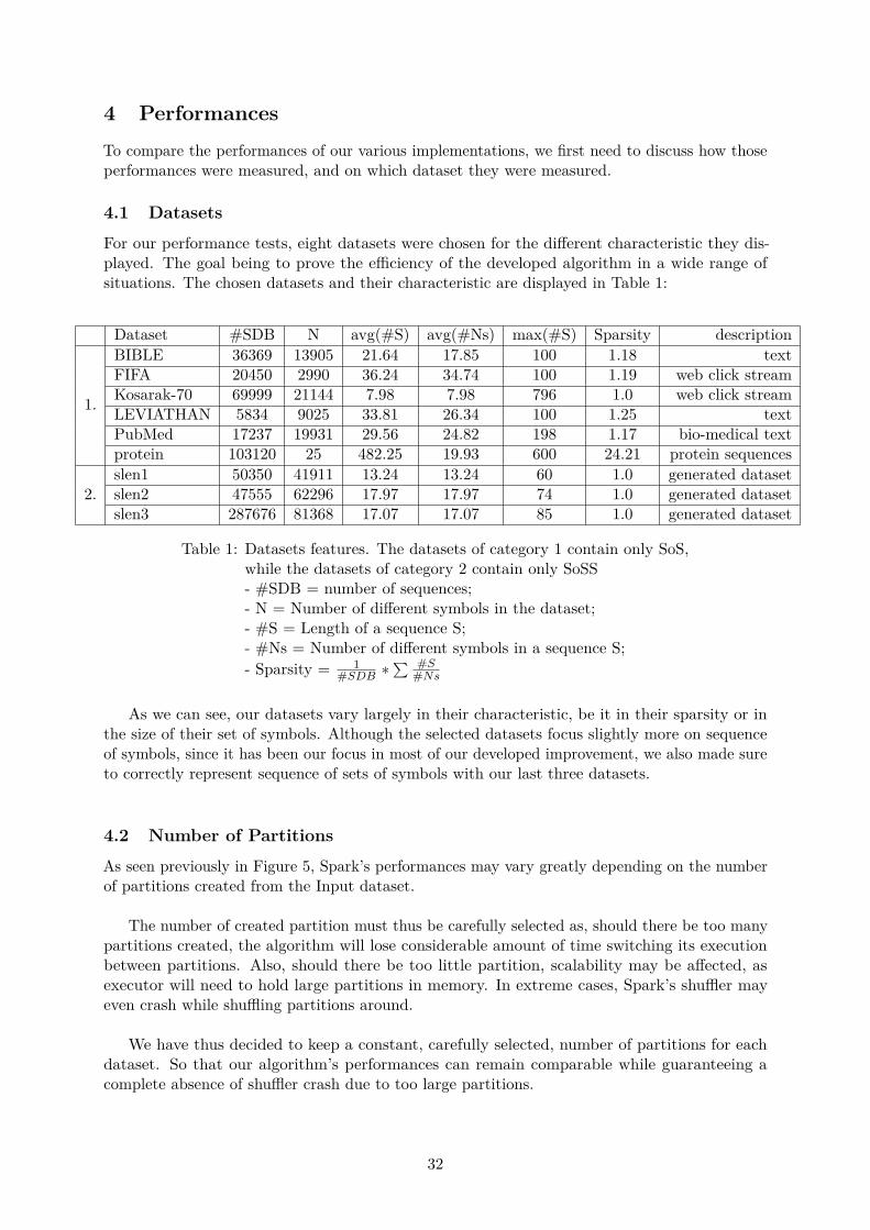
4 Performances

To compare the performances of our various implementations, we first need to discuss how thoseperformances were measured, and on which dataset they were measured.

4.1 Datasets

For our performance tests, eight datasets were chosen for the di�erent characteristic they dis-played. The goal being to prove the e�ciency of the developed algorithm in a wide range ofsituations. The chosen datasets and their characteristic are displayed in Table 1:

Dataset #SDB N avg(#S) avg(#Ns) max(#S) Sparsity description

1.

BIBLE 36369 13905 21.64 17.85 100 1.18 textFIFA 20450 2990 36.24 34.74 100 1.19 web click streamKosarak-70 69999 21144 7.98 7.98 796 1.0 web click streamLEVIATHAN 5834 9025 33.81 26.34 100 1.25 textPubMed 17237 19931 29.56 24.82 198 1.17 bio-medical textprotein 103120 25 482.25 19.93 600 24.21 protein sequences

2.slen1 50350 41911 13.24 13.24 60 1.0 generated datasetslen2 47555 62296 17.97 17.97 74 1.0 generated datasetslen3 287676 81368 17.07 17.07 85 1.0 generated dataset

Table 1: Datasets features. The datasets of category 1 contain only SoS,while the datasets of category 2 contain only SoSS- #SDB = number of sequences;- N = Number of di�erent symbols in the dataset;- #S = Length of a sequence S;- #Ns = Number of di�erent symbols in a sequence S;- Sparsity = 1

#SDB úq #S

#Ns

As we can see, our datasets vary largely in their characteristic, be it in their sparsity or inthe size of their set of symbols. Although the selected datasets focus slightly more on sequenceof symbols, since it has been our focus in most of our developed improvement, we also made sureto correctly represent sequence of sets of symbols with our last three datasets.

4.2 Number of Partitions

As seen previously in Figure 5, Spark’s performances may vary greatly depending on the numberof partitions created from the Input dataset.

The number of created partition must thus be carefully selected as, should there be too manypartitions created, the algorithm will lose considerable amount of time switching its executionbetween partitions. Also, should there be too little partition, scalability may be a�ected, asexecutor will need to hold large partitions in memory. In extreme cases, Spark’s shu�er mayeven crash while shu�ing partitions around.

We have thus decided to keep a constant, carefully selected, number of partitions for eachdataset. So that our algorithm’s performances can remain comparable while guaranteeing acomplete absence of shu�er crash due to too large partitions.

32

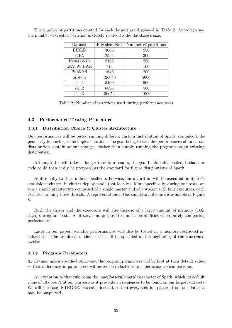
The number of partitions created for each dataset are displayed in Table 2. As we can see,the number of created partition is closely related to the database’s size.

Dataset File size (Ko) Number of partitionsBIBLE 3065 250FIFA 2594 300

Kosarak-70 2166 250LEVIATHAN 713 100

PubMed 1646 200protein 126046 5000slen1 5400 500slen2 6896 500slen3 39654 1000

Table 2: Number of partitions used during performance tests

4.3 Performance Testing Procedure

4.3.1 Distribution Choice & Cluster Architecture

Our performances will be tested running di�erent custom distribution of Spark, compiled inde-pendently for each specific implementation. The goal being to test the performances of an actualdistribution containing our changes, rather than simply running the program on an existingdistribution.

Although this will take us longer to obtain results, the goal behind this choice, is that ourcode could then easily be proposed as the standard for future distributions of Spark.

Additionally to that, unless specified otherwise, our algorithm will be executed on Spark’sstandalone cluster, in cluster deploy mode (not locally). More specifically, during our tests, werun a simple architecture composed of a single master and of a worker with four executors, eachexecutor running three threads. A representation of this simple architecture is available in Figure8.

Both the driver and the executors will also dispose of a large amount of memory (10Geach) during our tests. As it serves no purpose to limit their abilities when purely comparingperformances.

Later in our paper, scalable performances will also be tested in a memory-restricted ar-chitecture. The architecture then used shall be specified at the beginning of the concernedsection.

4.3.2 Program Parameters

At all time, unless specified otherwise, the program parameters will be kept at their default value,so that di�erences in parameters will never be reflected in our performance comparisons.

An exception to that rule being the ’maxPatternLength’ parameter of Spark, which its defaultvalue of 10 doesn’t fit our purpose as it prevents all sequences to be found on our largest datasets.We will thus use INTEGER.maxValue instead, so that every solution pattern from our datasetsmay be outputted.

33

Figure 8: The simple architecture used during the majority of our tests

Also, as mentioned previously, all additional functionalities implemented have been designedto a�ect performance as little as possible when left to their default value. Their default valuewill thus similarly be used, unless specified otherwise before the performance test.

4.3.3 Measurement Span

For our performance tests, we measure not only the running time of our algorithm, but also itspre-processing and dataset loading performances. The aim being to develop a new implementationthat entirely surpasses the old one.

4.4 Testing the Implementations

4.4.1 Comparing Spark and PPIC’s original implementations

Since PPIC is neither scalable nor concurrent, we exceptionally used an even simpler architecturefor our test on Spark, restraining our worker to a single executor so that both implementationcan work under equivalent resources.

As we can see in Figure 9, PPIC greatly overcomes Spark on nearly every dataset given thesame resources, the only exceptions being the Kosarak-70 and PubMed dataset.

We can however notice that, on those two datasets, PPIC’s performances are extremelystable. As we can see in the performance tests involving lower amount of supporting sequenceon PubMed, PPIC becomes the most e�cient in the long run. We have no doubt that a simi-lar situation would happen for Kosarak-70, should we have been PPIC the opportunity in our tests.

As said previously, the reason behind those stable performance lies in the required pre-processing of PPIC being quite long. The small di�erence we can see in those stable performancesare thus the running time of the main algorithm itself.

4.4.2 Performances of our First CP Based Implementation

As we can see in figure 10, this first implementation, which simple merges the two algorithmsby replacing Spark’s local execution by PPIC, is already much more e�cient on sequence ofsymbols problems than Spark’s original algorithm. We can however notice than the single-threadexecution of PPIC sometimes overcome our new scalable implementation, despite the lower

34

!—Test realised on a simplified architecture !—

PPIC: 1 thread with 10G memorySpark: 1 driver + 1 worker with 1 executor. 10G memory each

Figure 9: Original performances of PPIC and Spark

amount of resources at his disposal. The worst such case being protein, a dataset on which PPICremain far superior despite the lower resource it disposes, which may appear disconcerting atfirst glance.

Another disconcerting thing to notice may be the relative flatness of PPIC’s performancemeasurement. Making it seem as if the decrease in the amount of required support isn’t reallyfelt by the algorithm. On Kosarak and PubMed, the performances of PPIC remains worse by a10x factor which cannot be explained by the lack of resources alone. Similarly, on protein, theperformance of our new algorithm remain worse by a 10x factor, despite the additional resourcesgiven to its execution.

However, those oddities in our performance measurements are perfectly explainable, theyactually result from three major factors:

1. First, the pre-processing of the original PPIC algorithm wasn’t implemented e�ciently,

35

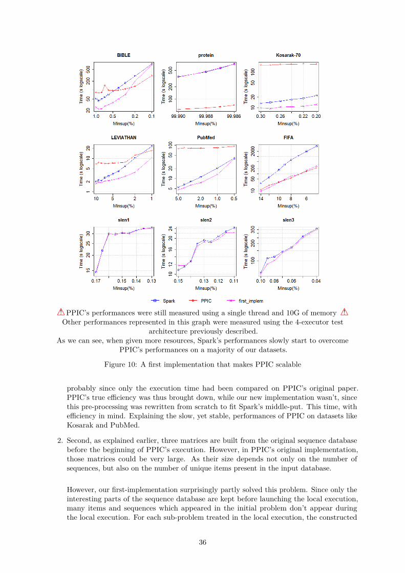
!—PPIC’s performances were still measured using a single thread and 10G of memory !—Other performances represented in this graph were measured using the 4-executor test

architecture previously described.As we can see, when given more resources, Spark’s performances slowly start to overcome

PPIC’s performances on a majority of our datasets.

Figure 10: A first implementation that makes PPIC scalable

probably since only the execution time had been compared on PPIC’s original paper.PPIC’s true e�ciency was thus brought down, while our new implementation wasn’t, sincethis pre-processing was rewritten from scratch to fit Spark’s middle-put. This time, withe�ciency in mind. Explaining the slow, yet stable, performances of PPIC on datasets likeKosarak and PubMed.

2. Second, as explained earlier, three matrices are built from the original sequence databasebefore the beginning of PPIC’s execution. However, in PPIC’s original implementation,those matrices could be very large. As their size depends not only on the number ofsequences, but also on the number of unique items present in the input database.

However, our first-implementation surprisingly partly solved this problem. Since only theinteresting parts of the sequence database are kept before launching the local execution,many items and sequences which appeared in the initial problem don’t appear duringthe local execution. For each sub-problem treated in the local execution, the constructed

36

matrices will thus be much smaller in size. Which explains further our new implementation’se�ciency gain on datasets with large amounts of distinct items.

3. Finally, our third major factor is a major ine�ciency that comes as a by-product of scal-ability. It appears mostly on datasets composed of a small number of repeated symbols,such as our protein dataset. In those cases, since the various sub-problems created beforeour local execution are actually very similar to each other, our new implementation willlose an important amount of time recreating the three input matrices before launchingcomputations on those nearly identical sequence databases. While the original PPICimplementation would create those matrices once and use them through the reminder ofthe execution.

Sadly, this problem cannot be dynamically fixed without seriously a�ecting scalability ore�ciency, as it would require us to compare the projection of multiple prefixes. This meansthat, either we would have to project the prefixes multiple time to obtain the results of thosecomparisons, either we would project it once and keep multiple version of the databaseduring comparison, which would be a disaster for memory consumption and scalability.

Fortunately, although a complete dynamic fix of the problem is impractical for the imple-mentation of a scalable and e�cient solution. It is possible to give users the possibilityto reduce or even negate the e�ects of this by-product ine�ciency, through giving themcontrol over the amount of sub-problem created. Since the less such sub-problems, the lessthose matrices will need to be recalculated.

In fact, Spark’s implementation already contains a way to control the number of sub-problems created, thanks to the ’maxLocalProjDBSize’ parameter. Stopping furthersub-problem creation from problems that are already below the inputted parameter valuein size. A more direct and precise way to control the amount of generated problems wasthus added among other functionalities in the Quicker-Start implementation.

On the other hand, we can notice that multi-item performance weren’t impacted at all. Whichis normal since the modification made only concerned single-item problems.

4.4.3 Performances of Quicker-Start

As we can see, very small gain in time are generally made. With the exception of the Kosarak-70,slen2 and slen3 datasets, which are our datasets possessing the largest number of unique itemsafter cleaning the database. At first, we believed those small losses of performances were due tothe delay needed to transfer the already calculated frequent items to the various executor beinglarger than the time needed to actually recalculate those items from the small cleaned database.It was only much later, when we added the slen3 dataset, that we realised this interpretationwas incomplete.

In the original implementation, since the items need to be recalculated, they will be recalcu-lated only on the sequences contained in the partitions of the executor. In this new version, weforce every executor to receive those items and to store prefixes object for them. Those objectsthen created will then be kept on the executor for the entirety of the execution as, should anRDD need to be recalculated, they would be a necessary input for their recreation.

Meaning that, when the number of items are large, this additional feature will require morememory usage, and more computation time to receive the items and their frequencies and create

37

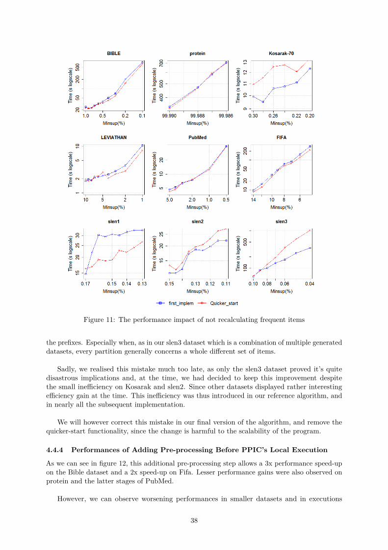
Figure 11: The performance impact of not recalculating frequent items

the prefixes. Especially when, as in our slen3 dataset which is a combination of multiple generateddatasets, every partition generally concerns a whole di�erent set of items.

Sadly, we realised this mistake much too late, as only the slen3 dataset proved it’s quitedisastrous implications and, at the time, we had decided to keep this improvement despitethe small ine�ciency on Kosarak and slen2. Since other datasets displayed rather interestinge�ciency gain at the time. This ine�ciency was thus introduced in our reference algorithm, andin nearly all the subsequent implementation.

We will however correct this mistake in our final version of the algorithm, and remove thequicker-start functionality, since the change is harmful to the scalability of the program.

4.4.4 Performances of Adding Pre-processing Before PPIC’s Local Execution

As we can see in figure 12, this additional pre-processing step allows a 3x performance speed-upon the Bible dataset and a 2x speed-up on Fifa. Lesser performance gains were also observed onprotein and the latter stages of PubMed.

However, we can observe worsening performances in smaller datasets and in executions

38

Figure 12: The performance impact of Database Pre-processing Before PPIC’s Execution

with larger minsup values. Theses losses however, pales in comparison to the performance gainobserved. Although at first glance they may seem large on log-scale graph, they do not evenexceed ten second, while the performance gains can be counted in hundreds of seconds on Bibleand Fifa.

The reason being those performance gains is that the larger the dataset and the lower theminimal amount of support, the longer prefixes will need to be before being executed locally.The larger those prefixes are before local execution, the more items can be cleaned from thesequences, the faster we can search the remains of those very sequences for patterns. Finally, iffewer items are present in our sequences during our local execution of PPIC, the three matricesneeded for PPIC’s execution can be created faster. Thus, hastening performance another fold.

However, cleaning sequences comes with a variable cost depending on the database size. If,much like Kosarak, the database only contains uncleanable sequences, performances will beslightly worsened. Of course, since this change is only applied before PPIC, the performancemeasured on our three slen datasets weren’t a�ected.

In the end, since such large increase in performances were observed, and since so many other

39

improvements needed to be tested, we decided to use the performance obtained here asreference for the remainder of this paper. To allow better comparison of performancesgains/losses, all further improvements were thus added to this version, and tested separately.Finally, by the end of this paper, a final version containing all changes providing performanceimprovements will be compiled into a single algorithm, algorithm whose performances will besimilarly tested.

4.4.5 Performances with Automatic choice of Local Execution

Figure 13: Performance improvement of recalculating ’maxItemPerItemset’ to avoidsearch for multi-item extension when unnecessary

As we can see on figure 13, this improvement achieves its goal with a slight performancedegradation, due to the need for calculating the ’maxItemPetItemSet’ value.

While, at first, we thought those small losses were worth this additional feature, as itguarantees the use of the much more performant PPIC. We, however, found soon after that therewas a more e�cient way to achieve the same goal, as you will see in the next section.

40

Figure 14: E�ciency gains of cleaning the sequence database before any local execution

4.4.6 Performances of Adding Pre-processing Before Any Local Execution

As we can see in figure 14, this implementation was, as expected, much more performant, forboth types of datasets.

Advantages are, however, lesser when mining sequences of sets of symbols, as the localexecution still relies on Spark’s implementation, which doesn’t take as much advantages of thisadditional cleaning step. The various improvement we made for cleaning sequences of symbols,on the other hand, are quite strongly reflected in these new performance measurement, surpassingour expectation on their e�ectiveness.

While, as said earlier, cleaning before the local execution allows us to detect witch algo-rithm should take charge the inputted database, another advantage also appeared. Should asub-problem from a database of sequence of sets of symbols become a database of sequence ofsymbols through cleaning, its local execution would be switched through PPIC, thus improvingthe significantly the performance on these projected database.

Sadly those cases should only appear rarely, and depend strongly on the inputted data. Still,it remains a nice addition to have, and which give occasional small boost to performances.

41

4.4.7 Performances with Position lists

Figure 15: Performance gain of first/last position lists

As we can see in Figure 15, the resulting performances of those three implementations weren’tconclusive. On every database of sequence of symbols but protein, which is a very sparse dataseton which this type of techniques excel, the modified algorithms delivered worse performancesthan our reference algorithm.

Those worsening performance appears because the benefit of those additional computationsimply do not have enough time to appear. After being calculated during the pre-processingstep, they only stay of use during the scalable execution of our algorithm. Since that, before thelocal execution, the sequence database will be compressed and the positions list will need to berecalculated.

Another reason for those worsening performance would be the transfer time of the calculatedpositions list, which can be very large depending on the number of frequent items. The delayimposed by their calculation and their transfer through the executors are thus far from negligible.

42

However, while su�ering from the same a�ictions, an improvement in performance can beobserved on databases of sequences of sets of symbols, where those techniques weren’t alreadyin use during the local execution stage. Especially on the slen1 dataset, where the measuredperformances improve significantly.

Despite the exception of the slen1 dataset, however, the measured performances gain does notjustify a nearly doubled memory consumption (nearly tripled in the case of the ’first_last_pos’improvement). Should no better implementation be found, this improvement should thus berestrained to only appear in Spark’s local execution, where additional memory consumptionwon’t a�ect data transfer times. Although the measured performances improvement would thusbe reduced, keeping such large RDD during the scalable execution step simply wouldn’t makesense for so little gains.

4.4.8 Performances with Specialised scalable execution

Figure 16: Performance improvement of specialising spark’s scalable stage.

As we can see on the slen datasets of Figure 16, this new implementation introduced a smallloss in performance for dataset of sequence of sets of symbols. As it needs to go through the

43

added detection but doesn’t profit of the advantages.

However, for sequences of symbols, performances improved greatly. Not only that, but thenew internal database representation make much more sense from a memory-consumption pointof view.

Thus, we judged these great advantages to be worth the slight loss of performance, anddecided to include this improvement in our final implementation.

4.4.9 Performances of Using Priority Scheduling for the Local Execution

4.4.9.1 Performances of Sorting Sub-Problems on the Reducer

Figure 17: Performance of a ’biggest problem first’ schedulingexecuted through the default sortBy() function of Spark.

As we can see in Figure 17, our first try at this implementation, impressive performanceimprovements can be observed, especially for the Kosarak, protein, slen2 and slen3 datasets.While BIBLE, FIFA and slen1 su�er from slight performance losses in their later stages, the

44

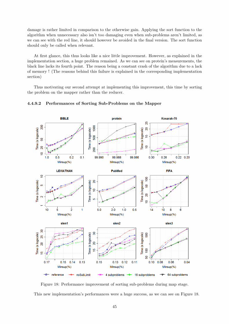
damage is rather limited in comparison to the otherwise gain. Applying the sort function to thealgorithm when unnecessary also isn’t too damaging even when sub-problems aren’t limited, aswe can see with the red line, it should however be avoided in the final version. The sort functionshould only be called when relevant.

At first glance, this thus looks like a nice little improvement. However, as explained in theimplementation section, a huge problem remained. As we can see on protein’s measurements, theblack line lacks its fourth point. The reason being a constant crash of the algorithm due to a lackof memory ! (The reasons behind this failure is explained in the corresponding implementationsection)

Thus motivating our second attempt at implementing this improvement, this time by sortingthe problem on the mapper rather than the reducer.

4.4.9.2 Performances of Sorting Sub-Problems on the Mapper

Figure 18: Performance improvement of sorting sub-problems during map stage.

This new implementation’s performances were a huge success, as we can see on Figure 18.

45

Not only have we obtained our previous boost in performance, we also successfully avoidedany memory consumption problem. This implementation advantages should thus be kept for thefinal version of our algorithm, since it allows far better performances when using the correct set.However, an automatic detection should be implemented, to detect when sorting sub-problemscould yield increased performances, and only sort in these circumstances.

4.4.10 Performances of using a Map Based Sequence Database Structure

Figure 19: Performance of a CP based algorithm replacingall three pre-processed matrices from PPIC by a Map structure

(Please take notice that we are here comparing performances with the original Sparkimplementation instead of the reference algorithm. Since the featured implementation doesn’tpossess the quicker-start improvement and the comparison is, in this case, much more relevant.)

As we can see in Figure 19, the performances of this implementation were terrible.

Profiling our algorithm revealed it came from two major factors. First, as feared, to attainthe same purpose as the three matrices with our map structure, we needed many more trailingpoints which had to be backtracked at each step of the search. Regularly generating significantperiods of time were our algorithm did nothing but backtrack the various sequences of its database.

46

The second factor was solution pruning. In PPIC, pruning our search space could be doneby checking the last positions of each item, quickly asserting that if the start of a sequencewas after the last position of an item in a sequence, the sequence was no longer supporting the item.

Here, however, the situation is di�erent. To e�ciently prune a multi-item pattern problem,checking the last position of items was no longer su�cient. To prune e�ciently, each item-setnow needed to be checked so that, should it match the current prefix, every possible extensionsin that item-set could be have their support increased.

Which amount to this algorithm doing twice the work for the same results. As we found outthrough our tests, pruning using PPIC’s original method (last position list) instead of fully, asspark did, produces better performance. A comparison of the two being available in the annexes,Figure 28.

Although the performances were better when not fully pruning our search space. Spark’soriginal local execution was still much more e�cient.

4.4.11 Performances PPIC with Partial Projection

The performance tests realised at the end of our implementation, shown in figure 20, revealedimproved e�ciency in comparison to Spark’s original algorithm and our previously created mapalgorithm on sequence of sets of symbols. On slen3, this implementation was even much moree�cient than any performances obtained earlier through the three position lists implementation.

These performances, however, came at the cost of an ine�ciency on datasets of sequences ofsymbols, where performances fail to overcome Spark’s standard on anything but the FIFA dataset.

This implementation should thus only be used for dealing with sets of symbols, while sequenceof symbols should be found through PPIC, whose e�ciency was focused on this kind of problem.

4.4.12 Performances of our final implementation

As we can see in Figure 21, our final implementation is much more performant than both our oldreference implementation, and the slightly improved ’Clean before any Local Execution’ imple-mentation. Surpassing previous performances on nearly every single dataset, but particularly onprotein and Kosarak-70 where the ’Specialised Scalable Execution’ improvement was extremelye�ective.

We can also observe that the performance loss brought from the quicker-start ’improvement’have disappeared on the concerned datasets. Improving performance further on our largestdatasets.

We a can, however, notice that performance worsens slightly on the slen1 dataset, a lightperformance loss easily explained by our choice to use our ’PPIC with Partial Projection’ im-plementation, which showed this exact same loss of performance on slen1, but much greaterperformance gain on slen3.

Finally we can observe that on the FIFA and BIBLE dataset, our performance tends towardthe performances of our ’Clean before any Local Execution’ implementation as the number ofrequired support gets lowered.

47

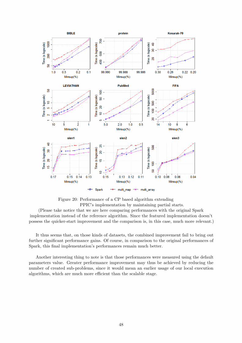
Figure 20: Performance of a CP based algorithm extendingPPIC’s implementation by maintaining partial starts.

(Please take notice that we are here comparing performances with the original Sparkimplementation instead of the reference algorithm. Since the featured implementation doesn’tpossess the quicker-start improvement and the comparison is, in this case, much more relevant.)

It thus seems that, on those kinds of datasets, the combined improvement fail to bring outfurther significant performance gains. Of course, in comparison to the original performances ofSpark, this final implementation’s performances remain much better.

Another interesting thing to note is that those performances were measured using the defaultparameters value. Greater performance improvement may thus be achieved by reducing thenumber of created sub-problems, since it would mean an earlier usage of our local executionalgorithms, which are much more e�cient than the scalable stage.

48

Figure 21: Performance of our final implementation

49

4.5 Scalability Tests

To conclude our performance testing section, let us measure the scalability of both Spark’soriginal implementation and of our final implementation.

The tests will be conducted as follows: We will run an architecture containing 1 driver (given5G memory to make sure all solution could be successfully received), and a variable number ofworkes. Each worker possessing one executor running a single thread, and disposing of only 1Gram memory.

Sadly, since the architecture on which we can run our tests has limited performances, runningmore than 10 workers will actually display slightly lowered performances, due to necessaryswitches between threads caused by an insu�cient number of cores. We will thus limit ourselvesto testing our implementation on architecture running 1,2,4, and 8 workers respectively, andcompare the resulting performances under those conditions.

Additionally, we had to specify a reduced value of 64000 for the ’maxLocalProjectedDatabas-eSize’ parameter whose default value is set at 32000000, as otherwise it could use too muchmemory during the local execution step and surpass the 1G ram allocated to our workers.

4.5.1 Scalability of the Original Implementation of Spark

As you may see on Figure 22, the original implementation of Spark scales really well up to acertain point. We can even notice that between 1,2, and 4 workers, doubling the number ofworkers means twice as good performances. However, this apparent linear scalability disappearswhen increasing the number of workers to 8 in our architecture, since few changes can be seen inour measured performances.

The original implementation of Spark is thus quite scalable, but has limitations beyond whatcan be justified by the limited performances of our architecture. More specifically, it appearsthat when dealing with greater number of executors, Spark gradually use more and more of itstime exchanging information instead of doing work. Thus the observed limitations.

4.5.2 Scalability of our final implementation

As you may see on Figure 23, our final implementation also shows greatly improved performancesin a scalable environment, in comparison to the original algorithm.

Although this implementation similarly shows reduced performance gain as the number ofworkers increase, it has been greatly mitigated. Our implementation is thus not only moreperformant in general, but also more scalable. Although not quite to the point of achieving truelinear scalability.

The greatest advantage of this new implementation being that we can launch the localexecution step faster if given more memory. We thus have a closer relation, beyond simple accesstime to the hard drive, between allocated memory and performances.

A default, however, would be that there is no way to allocate large sub-problems to executorsdisposing of extra amount of memory instead of other executor which would have more limitation.The ’maxLocalProjectedDatabaseSize’ parameter must thus be chosen while taking into accountthe lowest amount of memory available to an executor. Otherwise, the algorithm may crashduring the local execution stage due to insu�cient memory.

50

Figure 22: Scalability performances of the original implementation

51

Figure 23: Scalability performances of our final implementation

52

5 Conclusion

In this paper, we have developed a novel parallel sequential pattern mining approach based onconstraint programming modules that is both scalable and e�cient, greatly outperforming theoriginal implementation available on Spark.

To do so, we used a generic map-reduce based scalable PrefixSpan implementation to dividethe original problem in appropriately sized sub-problems. We then e�ciently solved thosesub-problems locally using a standard CP-solver running the PPIC algorithm for databases ofsequences of symbols, and a newly designed PPIC-like CP algorithm for database of sequences ofsets of symbols. Our various performance analysis then demonstrated that this novel approachnot only outperformed Spark’s original implementation in memory abundant environments, butalso on scalable memory limited environment.

Additionally, we also demonstrated that greater performances could be attained by limitingthe number of generated sub-problem depending on the provided number of executors and/or bysorting the generated sub-problems to compute larger sub-problems first. Finally, we demon-strated that cleaning large databases after operation large prefix projections allows noticeablee�ciency gain on the long run, as it reduces the time necessary to project prefixes during thelocal execution stage.

However, this novel approach still has an important flaw. While we have certainly demon-strated through the addition of multiple new functionalities that a certain level of modularityinherent to CP-solver was kept in this novel parallel algorithm. It remains a fact that using aCP-solver beneath Spark’s scalable framework isn’t as modular and flexible as an implementationfully englobed in a CP-solver.

The next step forward in progressing this research should thus be taken by incorporatingSpark’s parallel execution inside a CP framework. Thus allowing e�cient scalable execution onlarge scale databases and great modularity through the simple addition of constraints.

53

6 References

[1] N. R. Mabroukeh and C. I. Ezeife, “A taxonomy of sequential pattern mining algorithms,”ACM Computing Surveys (CSUR), vol. 43, no. 1, p. 3, 2010.

[2] R. Agrawal and R. Srikant, “Mining sequential patterns,” in Data Engineering, 1995.Proceedings of the Eleventh International Conference on, pp. 3–14, IEEE, 1995.

[3] R. Srikant and R. Agrawal, “Mining sequential patterns: Generalizations and performanceimprovements,” Advances in Database Technology—EDBT’96, pp. 1–17, 1996.

[4] M. J. Zaki, “Sequence mining in categorical domains: incorporating constraints,” in Pro-ceedings of the ninth international conference on Information and knowledge management,pp. 422–429, ACM, 2000.

[5] J. Pei, J. Han, B. Mortazavi-Asl, J. Wang, H. Pinto, Q. Chen, U. Dayal, and M.-C.Hsu, “Mining sequential patterns by pattern-growth: The prefixspan approach,” IEEETransactions on knowledge and data engineering, vol. 16, no. 11, pp. 1424–1440, 2004.

[6] B. Negrevergne and T. Guns, “Constraint-based sequence mining using constraint program-ming,” arXiv preprint arXiv:1501.01178, 2015.

[7] A. Kemmar, S. Loudni, Y. Lebbah, P. Boizumault, and T. Charnois, “A global constraintfor mining sequential patterns with gap constraint,” in International Conference on AIand OR Techniques in Constriant Programming for Combinatorial Optimization Problems,pp. 198–215, Springer, 2016.

[8] A. Kemmar, S. Loudni, Y. Lebbah, P. Boizumault, and T. Charnois, “Prefix-projectionglobal constraint for sequential pattern mining,” in International Conference on Principlesand Practice of Constraint Programming, pp. 226–243, Springer, 2015.

[9] M. J. Zaki, “Spade: An e�cient algorithm for mining frequent sequences,” Machine learning,vol. 42, no. 1, pp. 31–60, 2001.

[10] J. O. Aoga, T. Guns, and P. Schaus, “An e�cient algorithm for mining frequent sequencewith constraint programming,” in Joint European Conference on Machine Learning andKnowledge Discovery in Databases, pp. 315–330, Springer, 2016.

[11] OscaR Team, “OscaR: Scala in OR,” 2012. Available fromhttps://bitbucket.org/oscarlib/oscar.

[12] Z. Yang, Y. Wang, and M. Kitsuregawa, “Lapin: e�ective sequential pattern miningalgorithms by last position induction for dense databases,” Advances in Databases: Concepts,Systems and Applications, pp. 1020–1023, 2007.

[13] J. Deng, Z. Qu, Y. Zhu, G.-M. Muntean, and X. Wang, “Towards e�cient and scalable datamining using spark,” in Information and Communications Technologies (ICT 2014), 2014International Conference on. IET, pp. 1–6, 2014.

[14] M. J. Z. C.-T. Ho, “Large-scale parallel data mining,” edited by J. Siekmann J. G. Carbonell,Lecture Notes in Artificial Intelligence: Springer, 2000.

[15] J. O. Aoga, T. Guns, and P. Schaus, “Mining time-constrained sequential patterns withconstraint programming,” Constraint, pp. 1–23, 2017.

54

[16] M. Zaharia, M. Chowdhury, T. Das, A. Dave, J. Ma, M. McCauley, M. J. Franklin, S. Shenker,and I. Stoica, “Resilient distributed datasets: A fault-tolerant abstraction for in-memorycluster computing,” in Proceedings of the 9th USENIX conference on Networked SystemsDesign and Implementation, pp. 2–2, USENIX Association, 2012.

[17] T. Guns, S. Nijssen, and L. De Raedt, “Itemset mining: A constraint programming perspec-tive,” Artificial Intelligence, vol. 175, no. 12-13, pp. 1951–1983, 2011.

[18] J. Han, J. Pei, B. Mortazavi-Asl, H. Pinto, Q. Chen, U. Dayal, and M. Hsu, “Prefixspan:Mining sequential patterns e�ciently by prefix-projected pattern growth,” in proceedings ofthe 17th international conference on data engineering, pp. 215–224, 2001.

[19] Z. Yang and M. Kitsuregawa, “Lapin-spam: An improved algorithm for mining sequentialpattern,” in Data Engineering Workshops, 2005. 21st International Conference on, pp. 1222–1222, IEEE, 2005.

[20] F. Bonchi and C. Lucchese, “Extending the state-of-the-art of constraint-based patterndiscovery,” Data & Knowledge Engineering, vol. 60, no. 2, pp. 377–399, 2007.

[21] L. De Raedt, T. Guns, and S. Nijssen, “Constraint programming for itemset mining,” inProceedings of the 14th ACM SIGKDD international conference on Knowledge discoveryand data mining, pp. 204–212, ACM, 2008.

[22] L. De Raedt, T. Guns, and S. Nijssen, “Constraint programming for data mining andmachine learning,” in Proceedings of the Twenty-Fourth AAAI Conference on ArtificialIntelligence (AAAI-10), pp. 1671–1675, 2010.

[23] L. D. Raedt and A. Zimmermann, “Constraint-based pattern set mining,” in proceedings ofthe 2007 SIAM International conference on Data Mining, pp. 237–248, SIAM, 2007.

[24] J. Han, J. Pei, B. Mortazavi-Asl, Q. Chen, U. Dayal, and M.-C. Hsu, “Freespan: frequentpattern-projected sequential pattern mining,” in Proceedings of the sixth ACM SIGKDDinternational conference on Knowledge discovery and data mining, pp. 355–359, ACM, 2000.

[25] Q. Zhao and S. S. Bhowmick, “Sequential pattern mining: A survey,” ITechnical ReportCAIS Nayang Technological University Singapore, pp. 1–26, 2003.

55

7 Annexes

7.1 Glossary:

BFS breath-first search.

CP constraint programming.

DFS depth-first search.

PPIC Prefix Projection Incremental Counting propagator.

RAM random access memory.

RDD resilient distributed dataset.

SoS sequence of symbols.

SoSS sequence of sets of symbols.

SPM sequential pattern mining.

7.2 Additional example images

(a) S-matrix in original database (b) S-matrix in <AB>-projected database

S-M[a, b] = (4, 2, 2) => support(AB) = 4; support(BA) = 2; support((AB)) = 2;

Figure 24: Example of an S-matrix for PrefixSpan bi-level projection

7.3 Additional Performance Comparisons:

56

Figure 25: PPIC’s performances VS other specialized algorithm

57

Figure 26: Performance improvement of fixing Spark’s pre-processing

58

Figure 27: Performance improvement - soft limit on the number of created sub-problem.Tested on the reference (Clean Before Local Exec) implementation.

(P

59

Figure 28: Performance comparison of a full pruning VS a partial pruningon the multi_map implementation.

(Please take notice that we are here comparing to the original Spark implementation instead ofthe reference algorithm. Since the featured implementation doesn’t posses the early-start

improvement and the comparison is, in this case, much more relevant.)

60

7.4 Algorithms:

Algorithm 2: Prefix Projection Incremental Counting propagator (PPIC)Data: Given a sequence of symbol database (SDB), an array of reversible int representing

our search space (P), and minimal number of support (◊)Result: PPIC return the set of frequent sequence of symbol contained in SDB, such that

any returned pattern appear at least ◊ times in the database.// Init global param:

1 sids = [0, ..., len(SDB)]; poss = [0] * len(SDB);2 „ = 0; Ï = len(SDB)3 projFreq = Array such that projFreq[i] contains the number of sequence initially

supporting symbol i;4 Function propagate(SDB, P, i, ◊):

// espilon == special value that ends a valid pattern5 if Pi isBoundTo(epsilon) then

// A valid pattern has been found, fill remaining space to collect// P0 cannot be bound to epsilon

6 foreach j in i + 1, ..., L do7 P(j).assign(epsilon)8 end

/* When success is returned, the current pattern is collected asolution and we backtrack to the previous node of the searchtree. */

9 return Success10 else11 while Pi isBound and i < len(P) do12 nSupport = projectAndGetFreqs(SDB, P i, ◊, sids, poss, „, Ï)13 if nSupport < ◊ then

/* When failure is returned, we backtrack to the previous nodeof the search tree. */

14 return Failure15 end

// projFreq has been updated by the projectAndGetFreqs method.// Prune domain of Pi+1

16 pruneDomain(i + 1, projFreq)17 i++18 end19 end

/* When suspend is returned, we continue down the search tree. */20 return Suspend21 end

61

Algorithm 3: PPIC Continued1 Function projAndGetFreqs(SDB, itemToProject, ◊, sids, poss, „, Ï):2 projFreq[a] = 0 ’a œ {1, ..., nSymbols}3 i = „; j = „ + Ï; sup = 04 while i < „ + Ï do5 sid = sids[i]; pos = poss[i]; seq = SDB[sid]

/* pos => first position in a sequence, such that the previousprefix was supported. To project the new item, we only need tosearch the remains of the sequence. */

/* sid => The sequence id of a sequence which supported the previousprefix. */

/* sids => A vector starting at position „ and containing Ï elements,allowing to only search sequence that supported the previouspattern. */

/* seq => A sequence where the new item should be projected. */6 if lastPosMap(sid)(itemToProject) - 1 > pos then

// Find next position of itemToProject in seq7 if pos < firstPosMap(sid)(itemToProject) then

// Jump to first occurrence of the item in the sequence8 pos = firstPosMap(sid)(itemToProject)9 else

// Search for the next position of itemToProject10 while pos < len(seq) and itemToProject != seq[pos] do11 pos = pos + 112 end13 end

// item supported -> update projected database14 sids[j] = sid; poss[j] = pos + 1; j = j + 1; sup = sup + 1;15 posToCheck = interestingPosMap(sid)(pos) while posToCheck! = 0 do

// Faster than checking lastPosMap16 symbol = seq[posToCheck - 1] projFreqs[symbol] = projFreqs[symbol] + 1

posToCheck = interestingPosMap(sid)(posToCheck - 1)17 end18 end19 i = i+120 end21 „ = „ + Ï; Ï = sup22 return projFreqs23 end

62

Algorithm 4: Spark’s original implementation: Pre-ProcessingData: Given a sequence of sets of symbol database (SSDB), a minimal number of

supporting sequence (◊), a maximal pattern length (maxPatLen), and a maximallocal projected database size (maxLocalSize)

Result: Return the set of frequent sequence of sets of symbol contained in SDB. Such thatany returned pattern appear at least ◊ times in the database.

1 Function PreProcessing(SSDB, maxPatLen, maxLocalSize, ◊):// Clean database through a map reduce phase

2 freqItems = findFrequentItem(SSDB, ◊)3 cleanedSequences = cleanSequenceAndRenameItem(SSDB, freqItems)

// Find frequent sequences of sets of symbols4 solutionPatterns = scalableExecution(cleanedSequences, maxPatLen, maxLocalSize, ◊)

// Translate to original items name and Return5 return translateBackToOriginalItemsName(solutionPatterns)6 end

63

Algorithm 5: Spark’s original implementation: Scalable execution1 Function scalableExecution(SSDB, maxPatLen, maxLocalSize, ◊):

/* Encapsulate each sequence in a postfix, allowing to keep the currentposition and partial starts without copying the sequences. */

2 postfixes = SSDB.map(seq => PostFix(seq))// Init prefix list and solution list

3 solutionPatterns = Array.empty4 smallPrefixes = Array.empty5 largePrefixes = [prefix.empty]

// Start scalable execution6 while largePrefixes is not empty do7 mapReduceResults = postifixes.flatMap( postfix =>8 largePrefixes.flatMap( prefix =>9 extensions = postfix.project(prefix).findPrefixExtension()

10 extensions.map( (item, postfixSize) =>// Return a (key, value) pair

11 ((prefix.id, item), (1, postfixSize))12 )13 )14 ).reduceByKey((v1.1 + v2.1, v1.2 + v2.2)) // Aggregate values by key15 .filterByValue(v.1 Ø ◊) // Keep key-value pair with enough support

// Empty larger prefixes list16 largePrefixes.clean()

// Fill it with new, extended, prefixes17 foreach ((prefiID, extendingItem), (support, projDBSize) œ mapReduceResults do

// Create prefix, add it as solution18 newPrefix = largePrefixes.getByID(prefixID) += extendingItem19 solutionPatterns += newPrefix20 if len(newPrefix) < maxPatternLength then

// len(newPrefix) == number of non-zero item in prefix// zero == separator between item-sets

21 if projDBSize > maxLocalProjDBSize then22 largePrefixes += newPrefix23 else24 smallPrefixes += newPrefix25 end26 end27 end28 end29 if len(smallPrefixes) > 0 then

// For each prefix, project the whole database and solve locally30 toExecuteLocaly = postifixes.flatMap( postfix =>31 smallPrefixes.flatMap( prefix =>32 (prefix.ID, postfix.project(prefix).compress())33 )34 ).groupByKey().flatMap(sequences =>35 localExecution(sequences, maxPatLen - len(prefix), ◊)36 )37 end38 end

64

Algorithm 6: Spark’s original implementation: Local execution1 Function localExecution(SSDB, maxPatLen, ◊):2 if maxPatLen == 0 then3 return Array.empty4 end

// Find extending item that are sufficiently frequent5 counts = Map[Int, Int].empty.withDefaultValue(0)6 foreach postfix œ SSDB do7 foreach (extendingItem, size) œ postfix.findPrefixExtension() do8 counts(extending) += 19 end

10 end11 counts = counts.filterByValue(val Ø ◊)

// Extend for each item and continue searching12 solutions = ArrayList.empty[Prefix]13 foreach key œ counts do14 projectedDB = postfixes.project(key)15 foreach extension œ localExecution(projectedDB, maxPatLen-1, ◊) do16 solution += key + extensions17 end18 end19 return solutions20 end

65

Algorithm 7: Spark’s original implementation: Project and findPrefixExtension1 Class Postfix(sequence):2 start = 03 partialProjections = Array.empty4 Function project (Item):5 if start > len(sequence) then6 return7 end8 newPartialProjection = Array.empty9 if Item extends current Item-set in Prefix then

10 foreach partial œ partialProjections do11 newPos = findNextItemInCurrentItemSet(sequence, partial, Item)12 if Found Item in current ItemSet then13 newPartialProjection += newPos14 end15 end16 start = findSmallestPosition(newPartialProjection) + 117 else if Item start a new Item-set in Prefix then18 for Pos œ {start, ..., len(sequence) ≠ 1} do19 if sequence[Pos] == Item then20 if first found in loop then21 start = Pos + 122 else23 newPartialProjection += Pos24 end25 end26 end27 end28 partialProjections = newPartialProjection29 end30 Function project (Prefix):31 foreach Item œ Prefix do32 this.project(Item)33 end34 end35 Function project (findPrefixExtension):36 extendingItems = Set.empty37 foreach partial œ partialProjections do

// Find items that extend current itemSet38 extendingItems ++= findAllItemUntilNextSeparator(sequence, partial)39 end40 for Pos œ {start, ..., len(sequence) ≠ 1} do

// Find items that start a new itemSet41 extendingItems += sequence[Pos]42 end43 end44 end

66

Algorithm 8: First scalable CP based implementation1 Function

scalableExecution(SSDB, maxPatLen, maxLocalSize, ◊, hasSetsOfSymbols):/* Encapsulate each sequence in a postfix, allowing to keep the current

position and partial starts without copying the sequences. */2 postfixes = SSDB.map(seq => PostFix(seq))

// Init prefix list and solution list3 solutionPatterns = Array.empty4 smallPrefixes = Array.empty5 largePrefixes = [prefix.empty]

// Start scalable execution6 while largePrefixes is not empty do7 ... // Same as Spark’s original implementation8 end

// Start local execution9 if len(smallPrefixes) > 0 then

// For each prefix, project the whole database and solve locally10 toExecuteLocaly = postifixes.flatMap( postfix => smallPrefixes.flatMap( prefix =>11 (prefix.ID, postfix.project(prefix).compress())12 )).groupByKey().flatMap(sequences =>

// Use argument to determine which local execution to use13 if hasSetsOfSymbols then14 localExecution(sequences, maxPatLen - len(prefix), ◊)15 else16 sequences = removeSeparator(sequences)17 matrices = generatePPICMatrices()

/* PPIC will generate the P vector, add constraint to enforcemaxPatLen and then launch the execution, calling propagate inthe process. */

18 PPIC(sequences, maxPatLen - len(prefix), ◊, matrices)19 end20 )21 end22 end

67

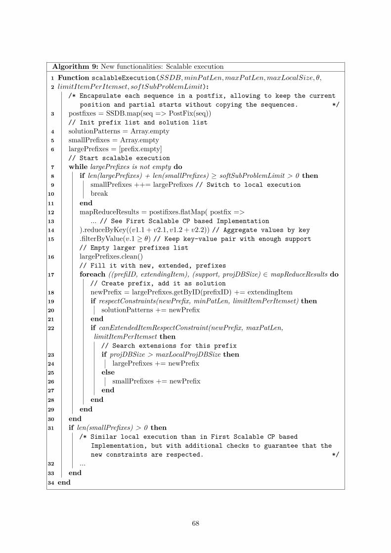
Algorithm 9: New functionalities: Scalable execution1 Function scalableExecution(SSDB, minPatLen, maxPatLen, maxLocalSize, ◊,2 limitItemPerItemset, softSubProblemLimit):



4 solutionPatterns = Array.empty5 smallPrefixes = Array.empty6 largePrefixes = [prefix.empty]

// Start scalable execution7 while largePrefixes is not empty do8 if len(largePrefixes) + len(smallPrefixes) Ø softSubProblemLimit > 0 then9 smallPrefixes ++= largePrefixes // Switch to local execution

10 break11 end12 mapReduceResults = postifixes.flatMap( postfix =>13 ... // See First Scalable CP based Implementation14 ).reduceByKey((v1.1 + v2.1, v1.2 + v2.2)) // Aggregate values by key15 .filterByValue(v.1 Ø ◊) // Keep key-value pair with enough support

// Empty larger prefixes list16 largePrefixes.clean()

// Fill it with new, extended, prefixes17 foreach ((prefiID, extendingItem), (support, projDBSize) œ mapReduceResults do

// Create prefix, add it as solution18 newPrefix = largePrefixes.getByID(prefixID) += extendingItem19 if respectConstraints(newPrefix, minPatLen, limitItemPerItemset) then20 solutionPatterns += newPrefix21 end22 if canExtendedItemRespectConstraint(newPrefix, maxPatLen,

limitItemPerItemset then// Search extensions for this prefix

23 if projDBSize > maxLocalProjDBSize then24 largePrefixes += newPrefix25 else26 smallPrefixes += newPrefix27 end28 end29 end30 end31 if len(smallPrefixes) > 0 then

/* Similar local execution than in First Scalable CP basedImplementation, but with additional checks to guarantee that thenew constraints are respected. */

32 ...33 end34 end

68

Algorithm 10: Quick - Start: Scalable execution1 Function scalableExecution(SSDB, minPatLen, maxPatLen, maxLocalSize, ◊,2 limitItemPerItemset, softSubProblemLimit, frequentItemAndCount):



4 solutionPatterns = Array.empty5 smallPrefixes = Array.empty6 largePrefixes = Array.empty7 foreach (item, count) œ frequentItemAndCount do8 largePrefixes += Prefix(item, count) // count == nbSupport for item9 end


// Project and extend prefix11 end12 if len(smallPrefixes) > 0 then

// Project and extend prefix locally13 end14 end

69

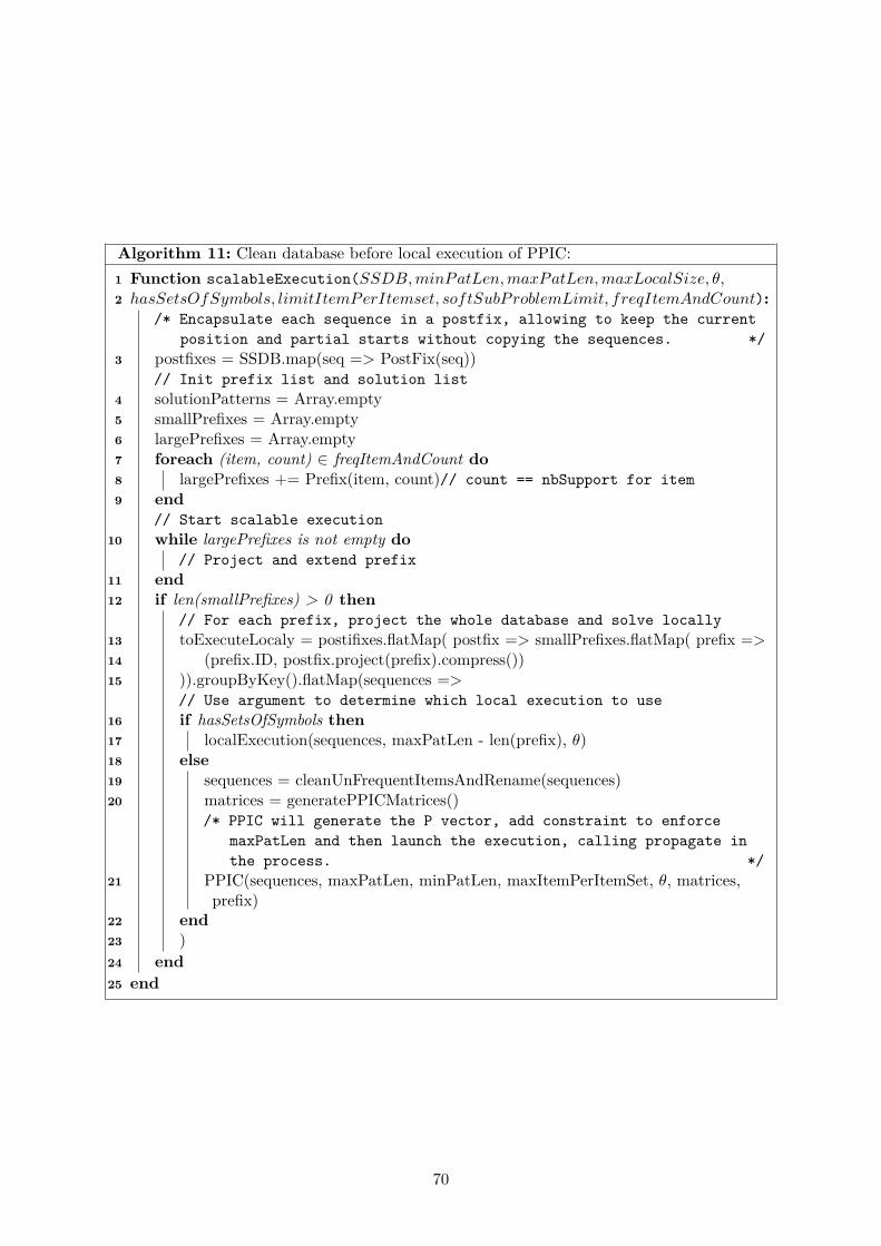
Algorithm 11: Clean database before local execution of PPIC:1 Function scalableExecution(SSDB, minPatLen, maxPatLen, maxLocalSize, ◊,2 hasSetsOfSymbols, limitItemPerItemset, softSubProblemLimit, freqItemAndCount):



4 solutionPatterns = Array.empty5 smallPrefixes = Array.empty6 largePrefixes = Array.empty7 foreach (item, count) œ freqItemAndCount do8 largePrefixes += Prefix(item, count)// count == nbSupport for item9 end




// Use argument to determine which local execution to use16 if hasSetsOfSymbols then17 localExecution(sequences, maxPatLen - len(prefix), ◊)18 else19 sequences = cleanUnFrequentItemsAndRename(sequences)20 matrices = generatePPICMatrices()


21 PPIC(sequences, maxPatLen, minPatLen, maxItemPerItemSet, ◊, matrices,prefix)

22 end23 )24 end25 end

70

Algorithm 12: Automatic Local Execution Selection:1 Function scalableExecution(SSDB, minPatLen, maxPatLen, maxLocalSize, ◊,2 limitItemPerItemset, softSubProblemLimit, freqItemAndCount):


3 postfixes = SSDB.map(seq => PostFix(seq))// Recalculate MaxItemPerItemset

4 calculatedMaxItemPerItemset = findLargestItemSetSize(SSDB)5 if limitItemPerItemset == 0 or limitItemPerItemset > calculatedMaxItemPerItemset

then6 limitItemPerItemset = calculatedMaxItemPerItemset7 end

// Init prefix list and solution list8 solutionPatterns = Array.empty9 smallPrefixes = Array.empty

10 largePrefixes = Array.empty11 foreach (item, count) œ freqItemAndCount do12 largePrefixes += Prefix(item, count) // count == nbSupport for item13 end




// Determine which local execution to use20 if calculatedMaxItemPerItemset > 1 then21 localExecution(sequences, maxPatLen - len(prefix), ◊)22 else23 sequences = cleanUnFrequentItemsAndRename(sequences)24 matrices = generatePPICMatrices()




71

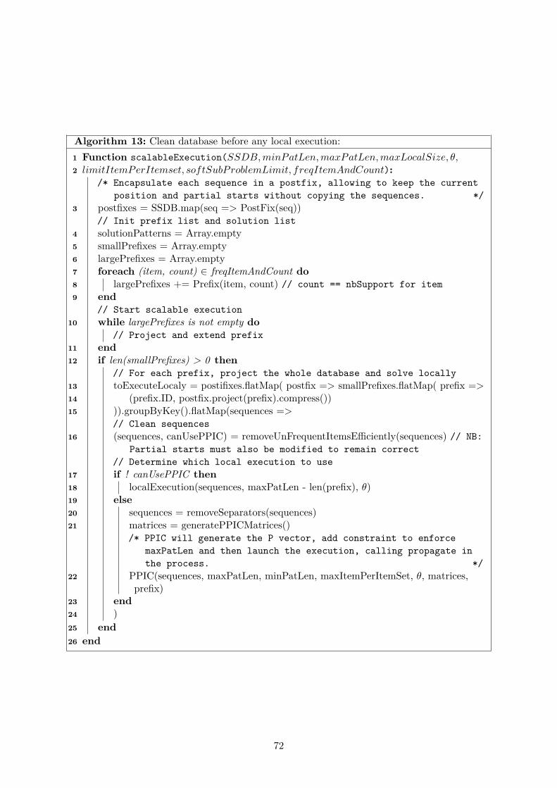
Algorithm 13: Clean database before any local execution:1 Function scalableExecution(SSDB, minPatLen, maxPatLen, maxLocalSize, ◊,2 limitItemPerItemset, softSubProblemLimit, freqItemAndCount):



4 solutionPatterns = Array.empty5 smallPrefixes = Array.empty6 largePrefixes = Array.empty7 foreach (item, count) œ freqItemAndCount do8 largePrefixes += Prefix(item, count) // count == nbSupport for item9 end




// Clean sequences16 (sequences, canUsePPIC) = removeUnFrequentItemsE�ciently(sequences) // NB:

Partial starts must also be modified to remain correct// Determine which local execution to use

17 if ! canUsePPIC then18 localExecution(sequences, maxPatLen - len(prefix), ◊)19 else20 sequences = removeSeparators(sequences)21 matrices = generatePPICMatrices()




72

Algorithm 14: Positions lists: Project and findPrefixExtension1 Class Postfix(sequence):2 start = 0; partialProjections = Array.empty3 firstPosList = getFirstPosList(sequence); lastPosList = getLastPosList(sequence)4 Function project (Item):5 if start > len(sequence) or start > lastPosList(Item) then6 return7 end

// Here, we know Item is present in remains of sequence8 newPartialProjection = Array.empty9 if Item extends current Item-set in Prefix then

10 foreach partial œ partialProjections do11 newPos = findNextItemInCurrentItemSet(sequence, partial, Item)12 if Found Item in current Item-set then13 newPartialProjection += newPos14 end15 end16 start = findSmallestPosition(newPartialProjection) + 117 else if Item start a new Item-set in Prefix then18 if start == 0 then19 start = firstPosList(sequence)20 end21 for Pos œ {start, ..., len(sequence) ≠ 1} do22 if sequence[Pos] == Item then23 if first found in loop then24 start = Pos + 125 else26 newPartialProjection += Pos27 end28 end29 end30 end31 partialProjections = newPartialProjection32 end33 Function project (Prefix):34 foreach Item œ Prefix do35 this.project(Item)36 end37 end38 Function project (findPrefixExtension):39 extendingItems = Set.empty40 foreach partial œ partialProjections do

// Find items that extend current itemSet41 extendingItems ++= findAllItemUntilNextSeparator(sequence, partial)42 end43 for (Item, lastPos) œ lastPosList, such that lastPos Ø start do44 extendingItems += Item45 end46 end47 end

73

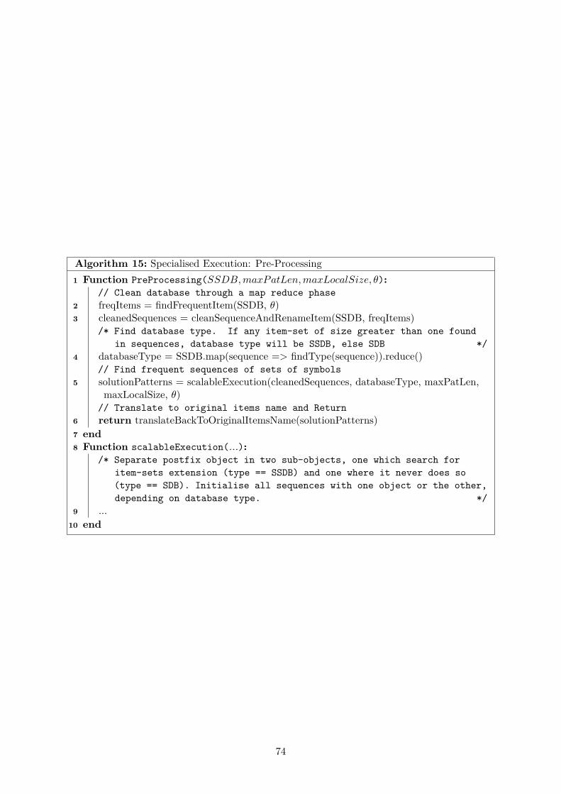
Algorithm 15: Specialised Execution: Pre-Processing1 Function PreProcessing(SSDB, maxPatLen, maxLocalSize, ◊):

// Clean database through a map reduce phase2 freqItems = findFrequentItem(SSDB, ◊)3 cleanedSequences = cleanSequenceAndRenameItem(SSDB, freqItems)

/* Find database type. If any item-set of size greater than one foundin sequences, database type will be SSDB, else SDB */

4 databaseType = SSDB.map(sequence => findType(sequence)).reduce()// Find frequent sequences of sets of symbols

5 solutionPatterns = scalableExecution(cleanedSequences, databaseType, maxPatLen,maxLocalSize, ◊)

// Translate to original items name and Return6 return translateBackToOriginalItemsName(solutionPatterns)7 end8 Function scalableExecution(...):

/* Separate postfix object in two sub-objects, one which search foritem-sets extension (type == SSDB) and one where it never does so(type == SDB). Initialise all sequences with one object or the other,depending on database type. */

9 ...10 end

74

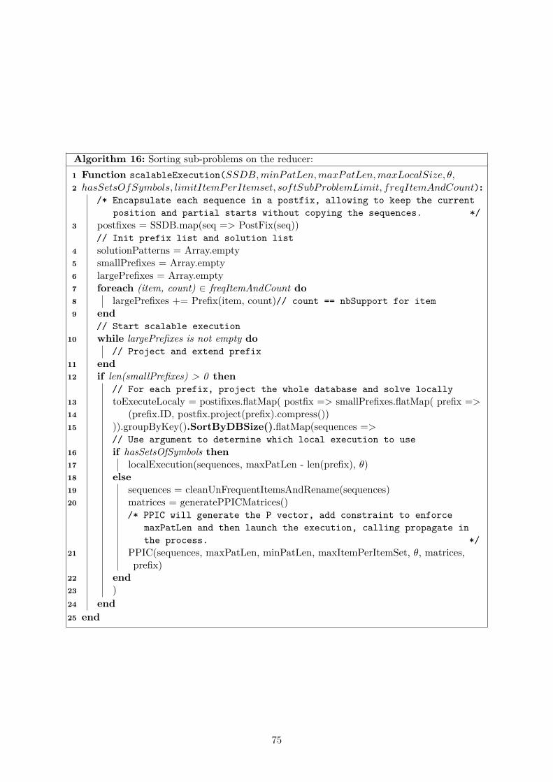
Algorithm 16: Sorting sub-problems on the reducer:1 Function scalableExecution(SSDB, minPatLen, maxPatLen, maxLocalSize, ◊,2 hasSetsOfSymbols, limitItemPerItemset, softSubProblemLimit, freqItemAndCount):



4 solutionPatterns = Array.empty5 smallPrefixes = Array.empty6 largePrefixes = Array.empty7 foreach (item, count) œ freqItemAndCount do8 largePrefixes += Prefix(item, count)// count == nbSupport for item9 end



// For each prefix, project the whole database and solve locally13 toExecuteLocaly = postifixes.flatMap( postfix => smallPrefixes.flatMap( prefix =>14 (prefix.ID, postfix.project(prefix).compress())15 )).groupByKey().SortByDBSize().flatMap(sequences =>





75

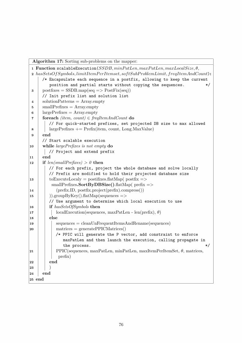
Algorithm 17: Sorting sub-problems on the mapper:1 Function scalableExecution(SSDB, minPatLen, maxPatLen, maxLocalSize, ◊,2 hasSetsOfSymbols, limitItemPerItemset, softSubProblemLimit, freqItemAndCount):



4 solutionPatterns = Array.empty5 smallPrefixes = Array.empty6 largePrefixes = Array.empty7 foreach (item, count) œ freqItemAndCount do

// For quick-started prefixes, set projected DB size to max allowed8 largePrefixes += Prefix(item, count, Long.MaxValue)9 end



// For each prefix, project the whole database and solve locally// Prefix are modified to hold their projected database size

13 toExecuteLocaly = postifixes.flatMap( postfix =>smallPrefixes.SortByDBSize().flatMap( prefix =>

14 (prefix.ID, postfix.project(prefix).compress())15 )).groupByKey().flatMap(sequences =>





76

Algorithm 18: PPIC with a Map based Structure (partial pruning):// Init global param:

1 ...2 Function propagate(SSDB, P, i, ◊):3 ... // Same propagate as PPIC, but the database is an SSDB instead4 end5 Function projAndGetFreqs(SSDB, itemToProject, ◊, sids, poss, „, Ï):6 projFreq[a] = 0 ’a œ {1, ..., nSymbols}; i = „; j = „ + Ï; sup = 07 while i < „ + Ï do8 sid = sids[i]; pos = poss[i]; seq = SSDB[sid]

// Get positions of itemToProject in sequence9 listSoughtItemPos = seq.get(itemToProject).discardItemsBefore(pos)

10 if not listSoughtItemPos.isEmpty() then// Find next position of itemToProject in seq

11 if lastItemInPwasSeparator()) then// Jump to first occurrence of the item in the sequence

12 pos = listSoughtItemPos.pop() + 1// item supported -> update projected database

13 sids[j] = sid; poss[j] = pos; j = j + 1; sup = sup + 1;14 else

/* Search the sequence Item-set by Item-set until all elementsof P’s current item-set match */

15 for position œ listSoughtItemPos do16 if curItemSetInSeqContainsAllItemOfCurrentItemSetInP(seq, position)

then// Jump to first occurrence of the item in the sequence

17 pos = listSoughtItemPos.pop() + 1// item supported -> update projected database

18 sids[j] = sid; poss[j] = pos; j = j + 1; sup = sup + 1;19 Break;20 end21 end22 end23 if itemToProject supported in sequence then

// Count support for items (partial pruning)24 foreach (item, positionsList) œ seq do25 positionList.discardItemsBefore(pos)26 if not positionList.isEmpty() then27 projFreqs[item] = projFreqs[item] + 128 end29 end

/* For full pruning, find all item-set in sequence thatsupport current Item-set in P, augment the projectedfrequency of all item present in those item-sets */

30 end31 end32 i = i+133 end34 „ = „ + Ï; Ï = sup35 return projFreqs36 end

77

Algorithm 19: PPIC with partial projections:1 Function projAndGetFreqs(SSDB, itemToProject, ◊, sids, poss, „, Ï, partialProj):2 projFreq[a] = 0 ’a œ {1, ..., nSymbols}; i = „; j = „ + Ï; sup = 03 while i < „ + Ï do4 sid = sids[i]; pos = poss[i]; seq = SSDB[sid]5 if itemToProject == separator then6 partialProj = Array.empty7 pos = findNextSeparatorInSequence(seq, pos)8 if pos < len(seq) then

// item supported -> update projected database9 sids[j] = sid; poss[j] = pos + 1; j = j + 1; sup = sup + 1;

10 projFreq = findFrequencyOfEachItemFromLastPosList(sid, pos)11 end12 else if partialProj.isEmpty then13 pos = firstPositionOfItemToProjectInRemainOfSequence(seq, pos)14 partialProj = AllSuccessivePosOfItemToProject(seq, pos)15 if pos < len(seq) then

// item supported -> update projected database16 sids[j] = sid; poss[j] = pos + 1; j = j + 1; sup = sup + 1;17 projFreq = findFrequencyOfEachItemFromLastPosList(sid, pos)18 end19 else20 newPartialProj = Array.empty21 foreach posToCheck œ partialProj do22 posToCheck = findPosOfNextItemToProjectInCurrentItemSet(seq,

posToCheck)23 if posToCheck < len(seq) then24 newPartialProj += posToCheck25 end26 end27 partialProj = newPartialProj28 pos = partialProj.min29 if not partialProj.isEmpty then

// item supported -> update projected database30 sids[j] = sid; poss[j] = pos + 1; j = j + 1; sup = sup + 1;31 projFreq = searchItemSetOfPartialProjForExtendingItem(seq, partialProj)32 end33 end34 i = i+135 end36 „ = „ + Ï; Ï = sup37 return projFreqs38 end

78

8 Acknowledgment

Computational resources have been provided by the Consortium des Équipements de CalculIntensif (CÉCI), funded by the Fonds de la Recherche Scientifique de Belgique (F.R.S.-FNRS)under Grant No. 2.5020.11

I would like to express my gratitude to my supervisor Pierre Schaus for the useful commentsand remarks that steered this thesis back in the right the direction when it was most needed.Furthermore, I would like to thank John Aoga for the continuous and unfailing support providedthrough the duration of this master thesis, and my readers: Guillaume Derval, Nijssen Siegfried,and Roberto D’Ambrosio, for their time and their valuable comments.

Rue Archimède, 1 bte L6.11.01, 1348 Louvain-la-Neuve www.uclouvain.be/epl

cp based sequence mining on the cloud using spark

Documents