cranfield university - ectinc.net vigueras gas turbine... · cranfield university ... the...
TRANSCRIPT
Cranfield University
Marco Osvaldo VIGUERAS ZUÑIGA
ANALYSIS OF GAS TURBINE COMPRESSOR FOULING AND WASHING ON LINE
School of Engineering
PhD
Cranfield University
SCHOOL OF ENGINEERING
PhD Thesis
2007
Marco Osvaldo VIGUERAS ZUÑIGA
ANALYSIS OF GAS TURBINE COMPRESSOR FOULING AND WASHING ON LINE
Supervisor: Professor Pericles Pilidis
Academic Year 2007 to 2008
© Cranfield University, 2007. All rights reserved. No part of this publication may be reproduced without the written permission of the copyright holder.
i
ABSTRACT
This work presents a model of the fouling mechanism and the evaluation of compressor
washing on line. The results of this research were obtained from experimental and
computational models.
The experimental model analyzed the localization of the particle deposition on the blade
surface and the change of the surface roughness condition. The design of the test rig was
based on the cascade blade arrangement and blade aerodynamics. The results of the
experiment demonstrated that fouling occurred on both surfaces of the blade. This
mechanism mainly affected the leading edge region of the blade. The increment of the
surface roughness on this region was 1.0 µm. This result was used to create the CFD
model (FLUENT). According to the results of the CFD, fouling reduced the thickness of
the boundary layer region and increased the drag force of the blade.
The model of fouling was created based on the experiment and CFD results and was
used to calculate the engine performance in the simulation code (TURBOMATCH).
The engine performance results demonstrated that in five days fouling can affect the
overall efficiency by 3.5%. The evaluation of the compressor washing on line was based
on the experimental tests and simulation of the engine performance. This system
demonstrated that it could recover 99% of the original blade surface. In addition, this
system was evaluated in a study case of a Power Plant, where it proved itself to be a
techno-economic way to recover the power of the engine due to fouling.
The model of the fouling mechanism presented in this work was validated by
experimental tests, CFD models and information from real engines. However, for
further applications of the model, it would be necessary to consider the specific
conditions of fouling in each new environment.
Keywords: Techno-economic, cascade blade, experiment, roughness, CFD

ii
ACKNOWLEDGEMENTS
Thank you GOD for the opportunity to do this postgraduate degree and for the
friendship of my family, professors and friends.
I would like to express my sincere thanks to The National Council for Science and
Technology of Mexico (CONACYT) for supporting my tuition and fees during this
Doctorate study and to the sponsors funding of this project: the Gas Turbine
Performance Engineering Group of Cranfield University and the company Recovery
Power Ltd.
iii
TABLE OF CONTENTS ABSTRACT ...................................................................................................................... i ACKNOWLEDGEMENTS ............................................................................................. ii TABLE OF FIGURES ................................................................................................... vii TABLE OF TABLES ..................................................................................................... xv TABLE OF EQUATIONS ........................................................................................... xvii 1 GENERAL INTRODUCTION ................................................................................ 1
1.1 Overview .......................................................................................................... 1 1.2 Thesis Structure ................................................................................................ 2 1.3 Importance of this study ................................................................................... 3 1.4 Previous Works ................................................................................................ 4
1.4.1 Gas turbine compressor fouling and washing on line............................... 4 1.4.2 Software description ................................................................................. 5
1.5 Thesis Objectives.............................................................................................. 6 1.6 Contribution...................................................................................................... 7
2 LITERATURE REVIEW......................................................................................... 8 2.1 Introduction ...................................................................................................... 8 2.2 Industrial Gas Turbines Performance Deterioration......................................... 8
2.2.1 Influence of the ambient condition in the gas turbine performance ......... 9 2.2.2 Types of deterioration in gas turbines .................................................... 10 2.2.3 Compressor degradation ......................................................................... 12 2.2.4 Combustion chamber degradation .......................................................... 12 2.2.5 Turbine degradation................................................................................ 12 2.2.6 Monitoring, simulation and diagnosis of gas turbines degradation........ 13
2.3 Compressor Fouling Mechanism.................................................................... 15 2.3.1 Fouling background................................................................................ 15 2.3.2 Filtration systems.................................................................................... 17 2.3.3 Fouling contaminant source.................................................................... 19
2.3.3.1 Sources of external contaminants ....................................................... 21 2.3.3.2 Sources of internal contaminants........................................................ 23 2.3.3.3 Steam and vapours as source of fouling ............................................. 23
2.3.4 Fouling in axial compressors.................................................................. 24 2.3.5 Gas turbine performance deterioration by fouling ................................. 25 2.3.6 Surface roughness change and aerodynamic consequences in blades.... 28
2.3.6.1 Boundary layer ................................................................................... 30 2.3.6.2 Surge margin ...................................................................................... 31 2.3.6.3 Compressor performance.................................................................... 32 2.3.6.4 Emissions............................................................................................ 34 2.3.6.5 Mechanical problems.......................................................................... 34
2.3.7 Previous fouling studies ......................................................................... 35 2.4 Compressor Washing...................................................................................... 37
2.4.1 Classification of compressor washing .................................................... 39 2.4.2 Cleaning fluids........................................................................................ 40 2.4.3 Cleaning fluid injection .......................................................................... 42 2.4.4 Cleaning fluid droplets ........................................................................... 43 2.4.5 Engine performance................................................................................ 45 2.4.6 Technical problems................................................................................. 46
iv
2.4.7 Compressor washing frequencies ........................................................... 47 2.5 Experimental Cascade Rig Tests .................................................................... 48
2.5.1 Flow Visualisation.................................................................................. 50 2.5.2 Turbulence .............................................................................................. 52 2.5.3 Boundary layer visualization.................................................................. 52 2.5.4 Pressures ................................................................................................. 52 2.5.5 Previous studies based on cascade blades .............................................. 54 2.5.6 Previous experimental studies of compressor fouling and washing....... 56
3 TEST RIG............................................................................................................... 59 3.1 Introduction .................................................................................................... 59 3.2 Experimental cascade blade............................................................................ 59
3.2.1 Particular Objective ................................................................................ 60 3.2.2 Background and source of information .................................................. 60
3.3 Test Rig Design .............................................................................................. 61 3.3.1 Axial compressor design (First stage) .................................................... 61 3.3.2 Cascade Blade Design ............................................................................ 69
3.3.2.1 Cascade geometry............................................................................... 71 3.3.3 Wind tunnel design (compressor)........................................................... 73
3.4 Test rig construction and installation.............................................................. 80 3.4.1 Industrial Fan.......................................................................................... 80 3.4.2 Bell Mouth.............................................................................................. 81 3.4.3 Inlet and Outlet sections ......................................................................... 82 3.4.4 Cascade................................................................................................... 82 3.4.5 Frame ...................................................................................................... 84 3.4.6 Instrumentation....................................................................................... 84
3.4.6.1 Temperature........................................................................................ 85 3.4.6.2 Humidity............................................................................................. 85
3.4.7 Test Rig Operation Instructions.............................................................. 86 4 EVALUATION OF CASCADE PERFORMANCE.............................................. 88
4.1 Introduction .................................................................................................... 88 4.2 The CFD study ............................................................................................... 88
4.2.1 Geometry ................................................................................................ 89 4.2.2 Boundary conditions............................................................................... 90 4.2.3 Mesh ....................................................................................................... 90 4.2.4 Model...................................................................................................... 94 4.2.5 Solver...................................................................................................... 94 4.2.6 Boundary conditions............................................................................... 94 4.2.7 Parameters of convergence..................................................................... 95
4.3 Performance evaluation of the test rig............................................................ 96 4.3.1 Conditions of operation of test rig.......................................................... 96 4.3.2 First configuration (6 blades) ............................................................... 100
4.3.2.1 Geometry .......................................................................................... 100 4.3.2.2 Experimental Results........................................................................ 101 4.3.2.3 CFD Results...................................................................................... 101 4.3.2.4 Discussion......................................................................................... 103
4.3.3 Second configuration (5 blades) ........................................................... 103 4.3.3.1 Geometry .......................................................................................... 103 4.3.3.2 Experimental Results........................................................................ 104
v
4.3.3.3 CFD Results...................................................................................... 104 4.3.3.4 Discussion......................................................................................... 106
4.3.4 Third configuration (4 blades and lateral walls)................................... 106 4.3.4.1 Geometry .......................................................................................... 106 4.3.4.2 Experimental Results........................................................................ 107 4.3.4.3 CFD Results...................................................................................... 107 4.3.4.4 Discussion......................................................................................... 108
4.4 Experimental validation of two dimensional flow ....................................... 109 4.4.1 Results for the 1st test of flow visualization test by oxide of titanium . 110 4.4.2 Results of flow visualization by wool trajectories................................ 111 4.4.3 Second test of flow visualization by oxide of titanium ........................ 111
4.5 Study of three dimensional flow effects in the cascade................................ 112 4.5.1 Three dimensional results of velocity and vortex................................. 113 4.5.2 Three dimensional results of pressure surfaces .................................... 113
4.6 Experimental validation of aerodynamic parameters with the CFD model . 115 4.6.1 Total Pressure Profiles and localization of wake.................................. 116 4.6.2 Boundary Layer analysis ...................................................................... 120
5 FOULING MODEL ............................................................................................. 126 5.1 Introduction .................................................................................................. 126 5.2 Preliminary experimental conditions............................................................ 126
5.2.1 The blade surface roughness................................................................. 127 5.2.2 Dust Sample Description ...................................................................... 130
5.3 Design of Fouling Injection System ............................................................. 131 5.3.1 Sections of the fouling injection system............................................... 131 5.3.2 Conditions of operation for the fouling system.................................... 132
5.4 Experimental results of fouling .................................................................... 134 5.4.1 First test (artificial powder) .................................................................. 135 5.4.2 Second test (artificial powder and glue agent-1) .................................. 136 5.4.3 Third test (artificial dust sample and glue agent-2).............................. 139 5.4.4 Fourth test (real dust sample and UW40-liquid oil) ............................. 140 5.4.5 Experimental results validation. ........................................................... 143
5.5 Experimental model of the fouling mechanism............................................ 147 5.5.1 Surface roughness changes................................................................... 147
5.5.1.1 Pressure Surface ............................................................................... 148 5.5.1.2 Suction Surface................................................................................. 149
5.5.2 Fouling Model ...................................................................................... 154 5.5.2.1 Mathematical model of fouling on the pressure surface of the blade154 5.5.2.2 Mathematical model of fouling on the blade suction surface........... 156
5.5.3 Boundary Layer Result......................................................................... 158 5.5.4 General discussion of fouling............................................................... 160
6 TECHNO-ECONOMIC STUDY OF COMPRESSOR FOULING AND WASHING ON LINE .................................................................................................. 162
6.1 Introduction .................................................................................................. 162 6.2 Aerodynamics of the blade affected by the fouling mechanism .................. 162
6.2.1 Static Pressure ...................................................................................... 162 6.2.2 Friction Skin Coefficient ...................................................................... 163 6.2.3 Drag force ............................................................................................. 164
6.3 Engine performance...................................................................................... 164
vi
6.3.1 Deterioration Factors ............................................................................ 165 6.3.2 Engine Performance Results................................................................. 166 6.3.3 Real case ............................................................................................... 168
6.4 Compressor washing on line......................................................................... 170 6.4.1 Experimental results of compressor washing on line ........................... 170 6.4.2 Engine performance simulation............................................................ 173
6.5 Techno-economic discussion........................................................................ 174 7 CONCLUSION AND RECOMMENDATIONS ................................................. 179
7.1 Conclusion.................................................................................................... 179 7.2 Recommendations ........................................................................................ 183
REFERENCES ............................................................................................................. 186 APPENDICES.............................................................................................................. 193
A. Engines specifications ...................................................................................... 193 B. Preliminary axial compressor design................................................................ 195 C. Computational simulation of gas turbine performance .................................... 199
vii
TABLE OF FIGURES Figure 1-1 Industrial Gas turbine cross section (Kurz and Brun, (2001))........................ 1 Figure 2-1 Output power of a gas turbine according to altitude and ambient temperature
(Mund (2006)). ....................................................................................................... 10 Figure 2-2 Mass flow of a gas turbine according to altitude and ambient temperature
(Mund (2006)). ....................................................................................................... 10 Figure 2-3 Representation of axial compressor performance map in three different
conditions: new, fouling and fouling with 1% of blockage factor (Kurz and Brun (2001)). ................................................................................................................... 15
Figure 2-4 Filter efficiency chart (Levine and Angello ( 2005)).................................... 17 Figure 2-5 EDX spectrum of layer deposit on the surface of compressor blades
(Kolkman (1993)). .................................................................................................. 20 Figure 2-6 Gas turbine configuration: two-shafts configuration (left), single-shaft
configuration (right). .............................................................................................. 28 Figure 2-7 Gas turbine efficiency based on deterioration in specific sections (Zwebek
(2002)) .................................................................................................................... 34 Figure 2-8 Mass flow reduction due to Fouling. (Saravanamuttoo and
Lakshminarasimha (1985))..................................................................................... 36 Figure 2-9 Washing system and cone nozzle (Kolev and Robben (1993)). ................... 38 Figure 2-10 Commercial systems of on line washing systems (Mund (2006)).............. 39 Figure 2-11 Typical nozzle locations and for online washing systems (Mund (2006)). 43 Figure 2-12 Result of the washing-fluid state due to temperature and pressure condition
(Mustafa (2006))..................................................................................................... 46 Figure 2-13 Representation of the flow visualization by smoke technique (Rubini
(2006)). ................................................................................................................... 51 Figure 2-14 Schematic of static tube ((Pankhurts, 1952)).............................................. 54 Figure 2-15 Three-dimensional flow effects (Saravanamuttoo, Cohen, and Rogers
(1996)). ................................................................................................................... 54 Figure 2-16 Low Reynolds cascade blade rig (Hobson, Hansen, Schnorenberg, and
Grove (2001)). ........................................................................................................ 56 Figure 2-17 Configuration of the NLR compressor rig test. Results from particles
removed by the washing process in the rig test (Kolkman (1993))........................ 57 Figure 3-1 First stage result of annulus diagram in the compressor design. .................. 65 Figure 3-2 Triangle of velocities in a cascade representation (Ramsden (2002)). ......... 68 Figure 3-3 Cascade blade row representation (velocities and angles), (Saravanamuttoo,
Cohen, and Rogers (1996))..................................................................................... 69 Figure 3-4 Middle section of cascade rotor (left). Annulus configuration and flow
streamline at middle section of first rotor (right) (Howell and Calvert (1978))..... 70 Figure 3-5 Results from the digital Image Technique (blade profile). ........................... 71 Figure 3-6 Middle section plane representation in a real blade row (Gostelow (1984)).72 Figure 3-7 Power and load curve for the Carter Howden centrifugal fan model HD77L.
................................................................................................................................ 74 Figure 3-8 Sketching of test rig: (1) Wind tunnel-inlet open to atmospheric conditions,
................................................................................................................................ 75 Figure 3-9 Diagram of the bell-mouth section design. Lateral View (left figure), Front
View (right figure).................................................................................................. 77
viii
Figure 3-10 Diagram of inlet section from the wind tunnel. Lateral View (left figure), Plan View (right figure).......................................................................................... 78
Figure 3-11 Diagram of cascade blade section. Lateral View (left figure), Plan View (right figure). .......................................................................................................... 79
Figure 3-12 Sketch diagram of the cascade blade section design. Lateral View (left figure), Plan View (right figure)............................................................................. 80
Figure 3-13 Electro-mechanical installation of the centrifugal fan model Carten Howden LTD in Test House 12. ........................................................................................... 81
Figure 3-14 Sample of the cloth-filter: efficiency of 90% for particles retention of 10µm, synthetic fiber media thickness of 10mm and pressure drop of 1% at low speeds (static filter)................................................................................................. 82
Figure 3-15 Manufacture of inlet-section (left) and outlet section (right) by the TIG welding process. ..................................................................................................... 82
Figure 3-16 Plane view of the cascade blade section (left), Isometric view of the cascade blade section (right). ............................................................................................... 83
Figure 3-17 Lateral view of the blade pressure surface (left), Isometric view of the blade (right). ..................................................................................................................... 83
Figure 3-18 Pressure transducer and electronic display (left). Screen from the DRUCK electronic display (left). The electronic display had pressure ranges of up to 700 bar with a precision of 0.15 mbar. .......................................................................... 85
Figure 3-19 Schematic representation of test rig and fan. Plan View (top), Lateral View (bottom) .................................................................................................................. 87
Figure 3-20 Photo from the Test Rig (Cranfield University Laboratory). ..................... 87 Figure 4-1 Unstructured mesh around the structured mesh in a compressor blade........ 91 Figure 4-2 Mesh at leading edge of the blade (left). Mesh at trailing edge of the blade
(right). ..................................................................................................................... 92 Figure 4-3 Layer treatment near to the wall region (Fluent 2005) ................................. 92 Figure 4-4 Schematic representation of test rig.............................................................. 98 Figure 4-5 Cascade Side view for total and static pressure measurements locations..... 98 Figure 4-6 Location of static pressure points in the inlet and outlet of the cascade....... 99 Figure 4-7 Variation of static Pressure at cascade inlet and different cascade velocities
.............................................................................................................................. 100 Figure 4-8 Sketch of cascade blade first configuration. ............................................... 100 Figure 4-9Manufacturing process of cascade blade first configuration. ...................... 100 Figure 4-10 Static pressure distribution at cascade inlet and outlet (6 blades
configuration) ....................................................................................................... 101 Figure 4-11 Results of CFD study for static pressure distribution (6 blades
configuration). ...................................................................................................... 102 Figure 4-12 Contours of Mach Number by the CFD analysis (6 blades configuration).
.............................................................................................................................. 103 Figure 4-13 Contours of Velocity Magnitudes by the CFD analysis (6 blades
configuration). ...................................................................................................... 103 Figure 4-14 Sketch of cascade blade second configuration. ........................................ 103 Figure 4-15 Manufacturing process of cascade blade second configuration................ 103 Figure 4-16 Static pressure distribution at cascade inlet and outlet (5 blades
configuration) ....................................................................................................... 104 Figure 4-17 Results of CFD analysis for the static pressure distribution (6 blades
configuration). ...................................................................................................... 105
ix
Figure 4-18 Contours of Mach Number by the CFD analysis (5 blades configuration)............................................................................................................................... 105
Figure 4-19 Contours of Velocity Magnitudes by the CFD analysis (5 blades configuration). ...................................................................................................... 105
Figure 4-20 Sketch of cascade blade third configuration ............................................. 106 Figure 4-21 Manufacturing process of cascade blade third configuration. .................. 106 Figure 4-22 Static pressure distribution at cascade inlet and outlet (4 blades
configuration). ...................................................................................................... 107 Figure 4-23 Results of CFD analysis for the static pressure distribution (4 blades
configuration). ...................................................................................................... 108 Figure 4-24 Contours of Mach Number by the CFD analysis (4 blades configuration).
.............................................................................................................................. 108 Figure 4-25 Contours of Velocity Magnitudes by the CFD analysis (4 blades
configuration). ...................................................................................................... 108 Figure 4-26 Application of mixture of TiO and Kerosene on blades to visualize the flow
path (pressure surfaces). ....................................................................................... 110 Figure 4-27 Application of mixture of TiO and Kerosene on blades to visualize the flow
path (suction surfaces). ......................................................................................... 110 Figure 4-28 1st test result of TiO flow visualization. The circle indicates the region that
was not modified by the flow path. ...................................................................... 110 Figure 4-29 Results of attaching pieces of wool to the blade surface in order to visualize
boundary separation.............................................................................................. 111 Figure 4-30 Flow trajectory visualization on pressure surface (left) and suction surface
(right) by TiO visualization. ................................................................................. 112 Figure 4-31 Flow trajectory visualization on the front leading edge (left) and outlet
passages (right) by TiO visualization. .................................................................. 112 Figure 4-32 Three dimensional Velocity Distribution ................................................. 113 Figure 4-33 Three dimensional Vorticity Distribution and blade wake location. ........ 113 Figure 4-34 Static Pressure Distribution in the middle section of the blade section in
study. .................................................................................................................... 114 Figure 4-35 Three dimensional distribution of the static pressure in the inlet section of
the wind tunnel. .................................................................................................... 114 Figure 4-36 Static Pressure Distribution on suction surface in three dimensional....... 114 Figure 4-37 Static Pressure Distribution on pressure surface in three dimensional..... 114 Figure 4-38Total Pressure Distribution suction surface three dimensional. ................ 115 Figure 4-39 Total Pressure Distribution pressure surface three dimensional............... 115 Figure 4-40 Representation of the cascade section in the CFD model and Lines of study
(30 lines). .............................................................................................................. 115 Figure 4-41 Representation of blade passage in the CFD mode (lines: 111, 113, 115,
117, 119, 121, 123, 125, 127, distance between each line 5mm)......................... 115 Figure 4-42 Test rig result of the total pressure distribution in Line 111 (inlet passage).
.............................................................................................................................. 116 Figure 4-43 CFD result of the total pressure distribution in Line 111 (inlet passage). 117 Figure 4-44 Test rig result of the total pressure distribution in Line 115 (inlet passage).
.............................................................................................................................. 117 Figure 4-45 CFD result of the total pressure distribution in Line 115 (inlet passage). 118 Figure 4-46 Test rig result of the total pressure distribution in Lines 123,129,131 ..... 118 Figure 4-47 CFD result of the total pressure distribution in Lines 123,129,131.......... 119
x
Figure 4-48 CFD result of the total pressure distribution in the 3rd passage. ............... 119 Figure 4-49 CFD result of the Velocity distribution in the 3rd passage........................ 120 Figure 4-50 CFD result of the Reynolds Number distribution in the 3rd passage. ....... 120 Figure 4-51 Boundary layer region represented by the velocity Profiles in the 3rd
passage (CFD result). ........................................................................................... 121 Figure 4-52 Velocity Profile of line-111 (inlet of the passage).................................... 121 Figure 4-53 Boundary layer region in the suction surface represented by the velocity
profile from Line-111. .......................................................................................... 122 Figure 4-54 Boundary layer represented by flow velocity profiles from 0 to 50% chord
of the blade on pressure surface. .......................................................................... 122 Figure 4-55 Boundary layer represented by flow velocity profile from 50 to 100% chord
of the blade on pressure surface ........................................................................... 123 Figure 4-56 Boundary layer represented by the flow velocity profile from 0 to 50%
chord of the blade at suction surface. ................................................................... 123 Figure 4-57 Boundary layer represented by the flow velocity profile from 50 to 100%
chord of the blade at suction surface. ................................................................... 124 Figure 5-1 Recorded data of the blade surface roughness by the instrument Surtronic-25
Taylor & Hobson. ................................................................................................. 127 Figure 5-2 Surface roughness result of experimental blades before polishing process
(suction surface). The Parameters calculated by mean of all the sampling lengths. A micro roughness filtering is used, with a ratio of 2.5 µm. Roughness Parameters, Gaussian filter, 0.8 mm was Ra=0.756µm. .......................................................... 128
Figure 5-3 Inchon Power Plant, South Korea (left), Didcot Power Plant, England UK (right) .................................................................................................................... 131
Figure 5-4 Fouling System lateral-view (left) and front-view (right). ......................... 132 Figure 5-5 Artificial powder deposition on suction surface after 7 hours of test rig
operation (injection rate of 100g/hr)..................................................................... 135 Figure 5-6 Artificial powder deposition on pressure surface after 7 hours of test rig
operation (injection rate of 100g/hr)..................................................................... 135 Figure 5-7 Artificial powder deposition on the leading edge (suction surface) after 7
hours of test rig operation (injection rate of 100g/hr). ......................................... 136 Figure 5-8 Artificial powder deposition on the leading edge (pressure surface) after 7
hours of test rig operation (injection rate of 100g/hr). ......................................... 136 Figure 5-9 Results of pressure surface deposition after 1hr of artificial powder injection
at rate of 100g/h. ................................................................................................... 137 Figure 5-10 Results of suction surface deposition after 1hr of artificial powder injection
at rate of 100g/h. ................................................................................................... 137 Figure 5-11 Results of pressure surface deposition after 2hr of artificial powder
injection at rate of 100g/h..................................................................................... 137 Figure 5-12 Results of suction surface deposition after 2hr of artificial powder injection
at rate of 100g/h. ................................................................................................... 137 Figure 5-13 Results of pressure surface deposition after 3hr of artificial powder
injection at rate of 100g/h..................................................................................... 138 Figure 5-14 Results of suction surface deposition after 3hr of artificial powder injection
at rate of 100g/h. ................................................................................................... 138 Figure 5-15 Results of pressure surface deposition after 4hr of artificial powder
injection at rate of 100g/h..................................................................................... 138
xi
Figure 5-16 Results of suction surface deposition after 4hr of artificial powder injection at rate of 100g/h. ................................................................................................... 138
Figure 5-17 Results of pressure surface deposition after 5hr of artificial powder injection at rate of 100g/h..................................................................................... 138
Figure 5-18 Results of suction surface deposition after 5hr of artificial powder injection at rate of 100g/h. ................................................................................................... 138
Figure 5-19 Results of pressure surface deposition after 6hr of artificial powder injection at rate of 100g/h..................................................................................... 139
Figure 5-20 Results of suction surface deposition after 6hr of artificial powder injection at rate of 100g/h. ................................................................................................... 139
Figure 5-21 Results of pressure surface deposition after 7hr of artificial powder injection at rate of 100g/h..................................................................................... 139
Figure 5-22 Results of suction surface deposition after 7hr of artificial powder injection at rate of 100g/h. ................................................................................................... 139
Figure 5-23 Test of liquid-grass as glue-agent in the deposition of artificial dust....... 140 Figure 5-24 Results of pressure surface deposition after 1hr of real dust sample injection
at rate of 100g/h. ................................................................................................... 141 Figure 5-25 Results of suction surface deposition after 1hr of artificial dust injection at
rate of 100g/h........................................................................................................ 141 Figure 5-26 Results of pressure surface deposition after 2hr of real dust sample injection
at rate of 100g/h. ................................................................................................... 141 Figure 5-27 Results of suction surface deposition after 2hr of artificial dust injection at
rate of 100g/h........................................................................................................ 141 Figure 5-28 Results of pressure surface deposition after 3hr of real dust sample injection
at rate of 100g/h. ................................................................................................... 142 Figure 5-29 Results of suction surface deposition after 3hr of artificial dust injection at
rate of 100g/h........................................................................................................ 142 Figure 5-30 Results of pressure surface deposition after 4hr of real dust sample injection
at rate of 100g/h. ................................................................................................... 142 Figure 5-31 Results of suction surface deposition after 4hr of artificial dust injection at
rate of 100g/h........................................................................................................ 142 Figure 5-32 Results of pressure surface deposition after 5hr of real dust sample injection
at rate of 100g/h. ................................................................................................... 142 Figure 5-33 Results of suction surface deposition after 5hr of artificial dust injection at
rate of 100g/h........................................................................................................ 142 Figure 5-34 Results of pressure surface deposition after 6hr of real dust sample injection
at rate of 100g/h. ................................................................................................... 143 Figure 5-35 Results of suction surface deposition after 6hr of artificial dust injection at
rate of 100g/h........................................................................................................ 143 Figure 5-36 Results of pressure surface deposition after 7hr of real dust sample injection
at rate of 100g/h. ................................................................................................... 143 Figure 5-37 Results of suction surface deposition after 7hr of artificial dust injection at
rate of 100g/h........................................................................................................ 143 Figure 5-38 Results of pressure surface deposition after 1hr of real dust sample injection
at rate of 100g/h. ................................................................................................... 143 Figure 5-39 Results of pressure surface deposition after 4hr of real dust sample injection
at rate of 100g/h. ................................................................................................... 143
xii
Figure 5-40. Results of pressure surface deposition after 5hr of real dust sample injection at rate of 100g/h..................................................................................... 143
Figure 5-41 Fouling on the IGV surface from the gas turbine of Inchon Power Plant, South Korea. ......................................................................................................... 144
Figure 5-42 Experimental result of fouling on the suction surface after 1hr of artificial dust injection at rate of 100g/h. ............................................................................ 144
Figure 5-43 Fouling found on the IGV suction surface (Didcot Power Plant, UK)..... 145 Figure 5-44 Experimental result of fouling on the suction surface after 2hr of dust
injection at rate of 100g/h..................................................................................... 145 Figure 5-45 Fouling found on the IGV pressure surface (Didcot Power Plant, UK). .. 145 Figure 5-46 Experimental result of fouling on the suction surface after 7hr of dust
injection at rate of 100g/h..................................................................................... 145 Figure 5-47 Fouling on the 1st rotor blade suction surface (Didcot Power Plant, UK).146 Figure 5-48 Experimental result of fouling on the suction surface after 1hr of dust
injection at rate of 100g/h..................................................................................... 146 Figure 5-49 Fouling on the 1st rotor blade pressure surface (Didcot Power Plant, UK).
.............................................................................................................................. 146 Figure 5-50 Experimental result of fouling on the suction surface after 1hr of dust
injection at rate of 100g/h..................................................................................... 146 Figure 5-51 Fouling distribution on blades of the 1st ,2nd, 3rd and 4th stages (Didcot
Power Plant, UK).................................................................................................. 147 Figure 5-52 Representation of particle deposition by the surface roughness parameter on
the pressure surface (µm) ..................................................................................... 149 Figure 5-53 Representation of particle deposition by the surface roughness parameter on
the suction surface (µm) ....................................................................................... 150 Figure 5-54 Fouling on the pressure surface in Region-1 during 7 hours at rate of 100g/h
of dust injection. ................................................................................................... 151 Figure 5-55 Fouling on the suction surface in Region-1 during 7 hours at rate of 100g/h
of dust injection. ................................................................................................... 151 Figure 5-56 Fouling on the pressure surface in Region-2 during 7 hours at rate of 100g/h
of dust injection. ................................................................................................... 151 Figure 5-57 Fouling on the suction surface in Region-2 during 7 hours at rate of 100g/h
of dust injection. ................................................................................................... 151 Figure 5-58 Fouling on the pressure surface in Region-3 during 7 hours at rate of 100g/h
of dust injection. ................................................................................................... 151 Figure 5-59 Fouling on the suction surface in Region-3 during 7 hours at rate of 100g/h
of dust injection. ................................................................................................... 151 Figure 5-60 Fouling on the pressure surface in Region-4 during 7 hours at rate of 100g/h
of dust injection. ................................................................................................... 151 Figure 5-61 Fouling on the suction surface in Region-4 during 7 hours at rate of 100g/h
of dust injection. ................................................................................................... 151 Figure 5-62 Fouling on the pressure surface in Region-5 during 7 hours at rate of 100g/h
of dust injection. ................................................................................................... 152 Figure 5-63 Fouling on the suction surface in Region-5 during 7 hours at rate of 100g/h
of dust injection. ................................................................................................... 152 Figure 5-64 Fouling on the pressure surface in Region-6 during 7 hours at rate of 100g/h
of dust injection. ................................................................................................... 152
xiii
Figure 5-65 Fouling on the suction surface in Region-6 during 7 hours at rate of 100g/h of dust injection. ................................................................................................... 152
Figure 5-66 Fouling on the pressure surface in Region-7 during 7 hours at rate of 100g/h of dust injection. ................................................................................................... 152
Figure 5-67 Fouling on the suction surface in Region-7 during 7 hours at rate of 100g/h of dust injection. ................................................................................................... 152
Figure 5-68 Fouling on the pressure surface in Region-8 during 7 hours at rate of 100g/h of dust injection. ................................................................................................... 152
Figure 5-69 Fouling on the suction surface in Region-8 during 7 hours at rate of 100g/h of dust injection. ................................................................................................... 152
Figure 5-70 Fouling on the pressure surface in Region-9 during 7 hours at rate of 100g/h of dust injection. ................................................................................................... 153
Figure 5-71 Fouling on the suction surface in Region-9 during 7 hours at rate of 100g/h of dust injection. ................................................................................................... 153
Figure 5-72 Fouling on the pressure surface in Region-10 during 7 hours at rate of 100g/h of dust injection. ....................................................................................... 153
Figure 5-73 Fouling on the suction surface in Region-10 during 7 hours at rate of 100g/h of dust injection. ....................................................................................... 153
Figure 5-74 Fouling on the pressure surface in Region-11 during 7 hours at rate of 100g/h of dust injection. ....................................................................................... 153
Figure 5-75 Fouling on the suction surface in Region-11 during 7 hours at rate of 100g/h of dust injection. ....................................................................................... 153
Figure 5-76 Fouling on the pressure surface in Region-12 during 7 hours at rate of 100g/h of dust injection. ....................................................................................... 153
Figure 5-77 Fouling on the suction surface in Region-12 during 7 hours at rate of 100g/h of dust injection. ....................................................................................... 153
Figure 5-78 Fouling on the pressure surface represented by the change of surface roughness (Ra=µm), location (region) and operation time (hour) at rate of 100g/h dust injection. ....................................................................................................... 154
Figure 5-79 Fouling on the suction surface represented by the changes of roughness (Ra), location (region) and operation time (hour) at rate of 100g/h dust injection............................................................................................................................... 156
Figure 5-80 Velocity profile in the 3rd passage represented from the Line-111 (transversal line at region 1) to Line-121 (transversal line at region 12). ............ 159
Figure 5-81 Boundary layer region represented by the velocity profile close to the pressure surface in region-1 (Line-111). .............................................................. 159
Figure 5-82 Boundary layer region represented by the velocity profile from the pressure surface in region-2 (Line-112).............................................................................. 159
Figure 5-83 Boundary layer region represented by the velocity profile close to the suction surface in region-1 (Line-111). ................................................................ 160
Figure 6-1 Static Pressure distribution on the pressure surface at dust rate injection of 100g/hr.................................................................................................................. 163
Figure 6-2 Static Pressure distribution on the suction surface at dust rate injection of 100g/hr.................................................................................................................. 163
Figure 6-3 Skin Friction Coefficient distribution on the pressure surface at dust rate injection of 100g/hr. ............................................................................................. 163
Figure 6-4 Skin Friction Coefficient distribution on the suction surface at dust rate injection of 100g/hr. ............................................................................................. 163
xiv
Figure 6-5 Reduction of the output power due to compressor fouling in a single shaft gas turbine according to the fouling rate (experiment 7 hors equivalent to 10 days in real engines)...................................................................................................... 167
Figure 6-6 Fuel consumption and overall efficiency performance due to compressor fouling in a single shaft gas turbine according to the fouling rate (experiment 7 hors equivalent to 10 days in real engines)........................................................... 167
Figure 6-7 Output power from the fouling model and real engine operation (single shaft gas turbine) ........................................................................................................... 168
Figure 6-8 Output powers from the real engine and from the fouling model scaled to 48 hours. .................................................................................................................... 169
Figure 6-9 Output power from the fouling model and real engine operation with the fouling model period scaled to 48 hours and the output power scaled to the maximum and minimum limits. ........................................................................... 169
Figure 6-10. Compressor washing system installed in the test rig. .............................. 171 Figure 6-11 Compressor washing on line operating in the test rig............................... 171 Figure 6-12 Top view of the cascade section during the washing on line process (test rig
in operation).......................................................................................................... 171 Figure 6-13 Surface of the blade during the process of washing on line (test rig in
operation).............................................................................................................. 172 Figure 6-14Washing-fluid before the cleaning process (left). Washing-fluid collected
from the cascade (right). ....................................................................................... 172 Figure 6-15 Pressure surface of the blades after the washing process (left). Pressure
surface of the blades after 1hour of dust injection at rate of 100g/hr equivalent to 1.5 day of engine operation (right). ...................................................................... 172
Figure 6-16 Suction surface of the blades after the washing process (left). Suction surface of the blades after 1hour of dust injection at rate of 100g/hr equivalent to 1.5 day of engine operation (right). ...................................................................... 173
Figure 6-17 Engine performance during fouling deterioration and power recovery by compressor washing each 10 days........................................................................ 174
Figure 6-18 Engine performance during fouling deterioration and power recovery by compressor washing each 2 days.......................................................................... 174
Figure 6-19 Fuel consumption results from the single shaft gas turbine simulation by two different washing frequencies........................................................................ 176
Figure 6-20 Accumulative sale of extra-electricity produced by compressor washing on line in millions of £............................................................................................... 177
xv
TABLE OF TABLES Table 2-1 Gas turbine location and typical contaminants (Mund and Pilidis (2004)). .. 21 Table 2-2 Common particle size and concentration in atmospheric air (Brumbaugh
(2002) & Giampolo (1997)). .................................................................................. 22 Table 2-3General environment scenarios of industrial gas turbines in operation. ......... 23 Table 2-4 Fouling distribution in a gas turbine compressor Frame-5 (Tarabrin,
Schurovsky, Bodrov, Stalder, and Bodrov (1998)) ................................................ 25 Table 2-5 Blades from the gas turbine Allison 501K..................................................... 29 Table 3-1. Information from the compressor section of the gas turbine model Saturn 20
................................................................................................................................ 61 Table 3-2 Characteristics of the compressor. *(Caterpillar (2005)) **(Ramsden (2002).
................................................................................................................................ 62 Table 3-3. Initial Chosen Variables. Source *(Caterpillar (2005), **(Ramsden (2002).62 Table 3-4 Inlet annulus dimensions for axial compressor design. ................................. 63 Table 3-5 Results of outlet annulus dimensions for an axial compressor design........... 64 Table 3-6 Results of the 1st stage annulus dimension for an axial compressor design... 64 Table 3-7 Triangle of velocities for inlet medium 1st rotor ........................................... 66 Table 3-8 Triangle of velocities for outlet medium 1st rotor ......................................... 66 Table 3-9 Summary of the inlet parameters of the axial design section 3.2.2................ 70 Table 3-10 Characteristics of the centrifugal fan model HD77L manufactured by Carten
Howden................................................................................................................... 73 Table 3-11 Characteristics of the three-phases electrical motor Alpak manufactured by
GEC Machines........................................................................................................ 73 Table 3-12 Fan inlet conditions (see figure 3-7). ........................................................... 74 Table 3-13 Summary of results for fan operating point (see Appendix-B).................... 76 Table 3-14 Filter media properties. ................................................................................ 78 Table 3-15 Characteristics of compressor axial blades used in the cacade blade. ......... 83 Table 3-16 Compact Digital Thermometer specifications ............................................. 85 Table 4-1 Mesh summary created in GAMBIT to be processed in FLUENT. .............. 93 Table 4-2 Wind Tunnel operation conditions................................................................. 97 Table 4-3 Measurements and calculation at different openings valve from the test rig. 99 Table 5-1 Specifications of Surtronic 25 (Taylor Hobson Ltd, 2001).......................... 128 Table 5-2 Surface roughness of the high pressure compressor blade manufactured by
Rolls Royce for the GT Trent 900. ....................................................................... 128 Table 5-3 Surface roughness of compressor blades manufactured by Siemens for the gas
turbine model V94.3A . ........................................................................................ 129 Table 5-4 Surface roughness of compressor blades prototype manufactured by Cranfield
University ............................................................................................................. 129 Table 5-5 Dust sample collected from the inlet filters of Inchon Power Plant in South
Korea. ................................................................................................................... 130 Table 5-6 Ideal scenarios of fouling rate for the Siemens V94.3A, Saturn 20 and Test
Rig. ....................................................................................................................... 134 Table 5-7 Results of artificial fouling from the artificial powder at rate of 100g/h ..... 137 Table 5-8 Results of artificial fouling from the real sample powder at rate of 100g/h 141 Table 5-9 Sources of information for real fouling on blades of industrial gas turbine
compressor............................................................................................................ 144

xvi
Table 5-10 Pressure surface roughness results on 12 regions at fouling rate of 100g/h............................................................................................................................... 148
Table 5-11 Suction surface roughness results on 12 regions at fouling rate of 100g/h.150 Table 6-1 Drag force force produced in the total surface at of 100g/h of dust injection
(fouling). ............................................................................................................... 164 Table 6-2 Increment of power due to the drag force. ................................................... 165 Table 6-3. Specifications of the single shaft industrial gas turbine.............................. 165 Table 6-4 Engine performance simulation at design point for the gas turbine............. 166 Table 6-5 British market of energy, source INNOGY Ltd 2003.................................. 175
xvii
TABLE OF EQUATIONS Equation 2-1 ................................................................................................................... 14 Equation 2-2 ................................................................................................................... 32 Equation 2-3 ................................................................................................................... 53 Equation 2-4 ................................................................................................................... 57 Equation 3-1 ................................................................................................................... 63 Equation 3-2 ................................................................................................................... 63 Equation 3-3 ................................................................................................................... 63 Equation 3-4 ................................................................................................................... 63 Equation 3-5 ................................................................................................................... 63 Equation 3-6 ................................................................................................................... 64 Equation 3-7 ................................................................................................................... 64 Equation 3-8 ................................................................................................................... 65 Equation 3-9 ................................................................................................................... 67 Equation 3-10 ................................................................................................................. 67 Equation 3-11 ................................................................................................................. 67 Equation 3-12 ................................................................................................................. 77 Equation 4-1 ................................................................................................................... 92 Equation 4-2 ................................................................................................................... 93 Equation 4-3 ................................................................................................................... 95 Equation 4-4 ................................................................................................................... 99 Equation 5-1 ................................................................................................................. 133 Equation 5-2 ................................................................................................................. 155 Equation 5-3 ................................................................................................................. 155 Equation 5-4 ................................................................................................................. 155 Equation 5-5 ................................................................................................................. 155 Equation 5-6 ................................................................................................................. 155 Equation 5-7 ................................................................................................................. 156 Equation 5-8 ................................................................................................................. 156 Equation 5-9 ................................................................................................................. 156 Equation 5-10 ............................................................................................................... 157 Equation 5-11 ............................................................................................................... 157 Equation 5-12 ............................................................................................................... 157 Equation 5-13 ............................................................................................................... 157 Equation 5-14 ............................................................................................................... 157 Equation 5-15 ............................................................................................................... 157 Equation 5-16 ............................................................................................................... 157 Equation 5-17 ............................................................................................................... 158 Equation 6-1 ................................................................................................................. 165 Equation 6-2 ................................................................................................................. 176
1
1 GENERAL INTRODUCTION
1.1 Overview
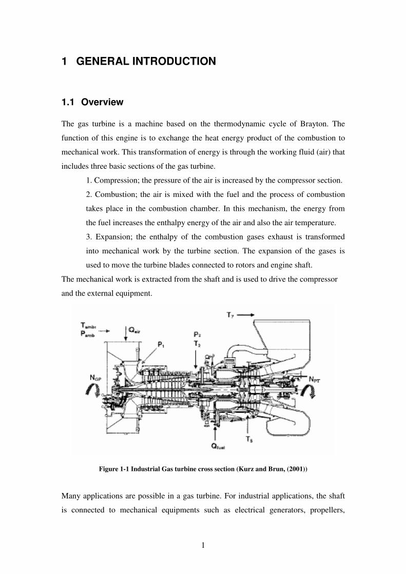
The gas turbine is a machine based on the thermodynamic cycle of Brayton. The
function of this engine is to exchange the heat energy product of the combustion to
mechanical work. This transformation of energy is through the working fluid (air) that
includes three basic sections of the gas turbine.
1. Compression; the pressure of the air is increased by the compressor section.
2. Combustion; the air is mixed with the fuel and the process of combustion
takes place in the combustion chamber. In this mechanism, the energy from
the fuel increases the enthalpy energy of the air and also the air temperature.
3. Expansion; the enthalpy of the combustion gases exhaust is transformed
into mechanical work by the turbine section. The expansion of the gases is
used to move the turbine blades connected to rotors and engine shaft.
The mechanical work is extracted from the shaft and is used to drive the compressor
and the external equipment.
Figure 1-1 Industrial Gas turbine cross section (Kurz and Brun, (2001))
Many applications are possible in a gas turbine. For industrial applications, the shaft
is connected to mechanical equipments such as electrical generators, propellers,

2
pumps, etc. For aero engine applications, the exhaust of the gases is used to produce
the thrust of the plane.
Industrial gas turbines are in operation around the world in many unfavourable
environments. So, it has been necessary to develop technologies to monitor the engine
performance in order to reduce the costs of operation and maintenance.
The problem of compressor fouling is considered as one of the most important and
common mechanism of degradation that affects the compressor performance. For that
reason auxiliary systems have been developed to eliminate this problem. This is the
case of compressor washing on line used frequently in industrial gas turbines.
The investigation presented in this thesis was focused on the fouling mechanism
based on experimental and computational results. In addition, the power recovery by
the compressor washing on line system was analyzed for the gas turbine application in
a Power Plant.
1.2 Thesis Structure
According to the nature of this project, it was decided to separate the thesis into two
main sections. The first section (Chapter 3, 4 and 5) presents a study of the fouling
mechanism and the blade aerodynamics. The second section (Chapter 6) presents the
application of this result in a real case to evaluate the engine performance and the
effectiveness of compressor washing on line.
Chapter 2 presents the theoretical bases of this research. An extensive search of
information from previous investigations has been summarized in this chapter.
Chapter 3 presents the design of the test rig based on real operational conditions. In
this chapter the details of the rig construction and the instrumentation specifications is
included.
3
Chapter 4 presents the validation of the experimental results based on a CFD model.
In this chapter, the configuration from the test rig is analyzed by a three dimensional
CFD model.
Chapter 5 presents the most important contribution of this research that is the
experimental results of the fouling mechanism. The mathematical model was created
based on the localization of particle deposition on the blade surface and the changes
produced in the surface roughness. In addition, this model was used to study the
changes of the blade aerodynamics.
Chapter 6 presents a techno-economic study of the engine operation affected by the
fouling mechanism and the effectiveness of compressor washing on line.
1.3 Importance of this study
According to the literature review, the effect of fouling has been associated in
previous studies with arbitrary factors from the output power of the engines.
However, the mechanism of fouling should be associated with the real physical
problems (modification of blade surfaces and blade aerodynamics).
The importance of this problem is illustrated in the following techno economic
example. The annual production in a gas turbine of 240MW/h (Power Plant) is
2,120,000 MWh per year1, this value represents 106 million USD of electricity sale
per year. If fouling affects 1% the compressor pressure ratio during a period of 4 years
(normal period of the engine overall maintenance), the engine has not produced
520,000MWh. This value represents 26 million USD of electricity that was not sold.
For that reason, companies and governments are interested in studying the
deterioration mechanism in industrial gas turbines to be competitive in the energy
market. A combination of this effort is this research sponsored by the Mexican
Government (CONACYT), Cranfield University (institution leader in gas turbine
1 Price Retail of 1MWh =50 USD
4
development) and the company Recovery Power Ltd (leader in technology of
compressor washing on line).
1.4 Previous Works
1.4.1 Gas turbine compressor fouling and washing on line
Fouling is commonly found in compressor blades, but the information about this topic
is very limited in the literature. According to the literature review, fouling has been
studied since 1980 with simple arbitrary factors linked with the output power of the
engine. However, this mechanism of degradation involves some other important and
relevant changes in the blade aerodynamics.
This thesis has settled its basis from the work produced by the Gas Turbine
Performance Engineering Group (GTPE) in Cranfield University in the last ten years.
In particular the topic of compressor washing on line has been studied by this group
with the participation of the company Recovery Power Ltd. Two previous PhD
investigations were presented about numerical CFD analysis of compressor washing
on-line (Mund (2006) and Mustafa (2006)). The water droplets distribution in the inlet
bell mouth was analyzed by Mund (2006), while the droplets trajectory was analyzed
by Mustafa (2006). In both projects the necessity to validate the results with
experimental models was mentioned.
The experimental study is the new area explored in this investigation of the Gas
Turbine Performance Engineering Group under the supervision and help of Professor
Pilidis (director of the project). The experimental work was done with the
participation and help of Angel Hernandez (MSc-candidate) and Dimitrios Foulfias
(PhD-candidate) and with the technical support of Paul Lambart, Ross Gordon and
Andy Lewis from the company Recovery Power Ltd. The writing work of this thesis
was done with the help of Miss Ruth Joy.
5
1.4.2 Software description
The improvements in the computational technology offer the opportunity to solve a
complex numerical model. Today, it is possible to solve “n” number of equation
systems with “n” number of variables in a reasonable computational time. This is the
case of the Computational Fluid Dynamics (CFD) algorithms. The CFD produces a
numerical solution from the Navier-Stokes equations. This computational application
was used to analyze the flow in this research by the program FLUENT.
FLUENT is a powerful state of the art code that solves computational fluid dynamics
models (fluid flow or heat transfer). The program was written in C program language
and it has the capacity to process complex geometries with structured and
unstructured meshes in two or three dimensional models. In this research, the
geometry was created by AUTOCAD (Computational Aided Design package) and the
mesh was created by GAMBIT.
The engine performance was studied from results obtained in the simulation program
of TURBOMATCH. This program was written in FORTRAN in Cranfield University
and it was designed to handle the thermodynamic gas turbine performance (Mund
(2006)). This code can include new subroutines to simulate different engine
configurations. The library of the program includes nine compressor maps and nine
turbines maps to calculate design or off design point of the engine operation. With the
use of pre-programmed routines called “codewords” and “bricks” it is possible to
calculate the engine performance degradation. The result from the engine
performance is presented by the internal parameters of output power, fuel
consumption, overall efficiency, etc.
The parameters that change the engine performance in the simulation code were
calculated with the computational tool of gas path analysis (GPA). The codes of GPA
link the physical fault of the engine with the internal parameters. The solution is
generated based on a matrix that includes independent and dependent parameters. In
general, there are two basic algorithms involved in the solution (fault tree and fault
matrix). The fault tree algorithm is a mechanical decision based on the output value
that converges in a possible fault. The fault matrix algorithm compares the values
6
from two variables (inputs and outputs values). In addition, the deviation of these
parameters from the failure can predict the quantity of the damage.
The code selected for the gas path analysis was the program GOTRESS. This
software was programmed in FORTRAN (Cranfield University) to predict the internal
engine parameters from faults implanted in the engine components. The program is
based on the matrix method in order to load multiple faults (input values). An
important characteristic of this program is the non linear application that it decreases
the errors produced by the numerical solution. The dependent parameters have to be
known and the number of independent parameters has to be equal or less than the
dependent parameters.
1.5 Thesis Objectives
The objective of this thesis was created based on the following conclusions based on
the literature review:
i. The mechanism of fouling in gas turbine compressors has not been studied
in detail.
ii. The cascade blade application offers a possibility to study the effect of the
blade aerodynamics and the mechanism of fouling.
iii. Experimental information of compressor washing on line is required to
validate previous theoretical studies.
Therefore, this PhD research has as its objective to obtain a model to predict the
fouling in gas turbine compressor blades.
To achieve with this objective, it is necessary to establish the following particular
objectives.
i. Specification of operation conditions from industrial gas turbine.
ii. Design of the test rig based on the blade aerodynamics.
iii. Analysis of blade aerodynamics due to modifications on the blade surface
roughness (fouling).

7
iv. Validation of experimental results with CFD models and information from
the real engine.
v. Analysis of gas turbine performance based on compressor fouling.
vi. Techno economic study of compressor washing on line in a Power Plant.
1.6 Contribution
The result of this research will show for the first time experimental information about
the fouling mechanism. The results from the CFD will present the effects of the blade
aerodynamics due to changes on the surface roughness. The performance of the gas
turbine will demonstrate the importance of fouling and compressor washing on line by
a techno economic analysis for industrial gas turbine application.
8
2 LITERATURE REVIEW
2.1 Introduction
In this chapter is summarized the relevant information published in the literature
linked with the topic of this research. Divided in four topics, the information is
presented with the following order. First section presents a general background of the
gas turbine and the common deterioration mechanisms that affect the engine
performance. The second section includes the previous studies of the mechanism of
fouling in the compressor. It will be important to note that information published at
the end of the seventies has been used to represent the problem of fouling for many
years linked only to the output power of the engine. The third section comments the
process of compressor washing online that it is used to eliminate the problem of
fouling in gas turbines. The final section describes previous experimental works of
cascade blades.
2.2 Industrial Gas Turbines Performance Deterioration
The deterioration of industrial gas turbines has been studied since 1914 when the ideal
cycle of Brayton was modified to represent the real conditions ((Horlock, 1992)). At
the end of the forties was observed that the gas turbine deterioration affected the
power production and increased the fuel consumption ((Zwebek, 2002)). During the
sixties the improvements in different sections of the gas turbine increased the engine
efficiency by 17% with pressure ratio of 7:1 and temperatures of 815ºC ((Boyce and
Gonzalez, 2005)). The increment of the fuel price in the seventies obligated to the gas
turbine users to study new ways to reduce the costs of operation. During this period
the deterioration mechanisms that affect the engine performance were classified
((Williams, 1981)). The boom of industrial gas turbines was in the eighties with the
installation of Combined Cycles in power plants. The results of new technologies at
the end of this decade increased the engine efficiency to 42% ((Zwebek, 2003)).
Today it is possible to find public documents published by OEM’s where the gas
turbine operates with efficiency of 45% and temperatures of 1371ºC (Boyce and
9
Gonzalez (2005)). However, these results are produced in special conditions (ISA*
conditions) and when the engine condition is new, because the gas turbine is a
machine that presents a quick degradation (Zwebek and Pilidis (2004)).
2.2.1 Influence of the ambient condition in the gas turbine performance
The airflow plays an important role in the gas turbine performance. The high quantity
of air required by the engine in a typical compressor is 500kg of air for each unit of
horse power produced by the engine (Zwebek and Pilidis (2003)). Previous
publications have demonstrated that optimal conditions of the air can produce high
levels of power production from the gas turbine with a low fuel consumption
(Weisman and Eckart (1985) & Zwebek and Pilidis (2004)).
The different applications of industrial gas turbine involve different conditions of the
air due to atmospheric conditions (Mund and Pilidis (2004)). For example, the
increment of a centigrade degree from the ambient temperature can produce that the
output power decreases 2% (see Figure 2-1) (Mund (2006)). The altitude also plays an
important factor in the engine performance. The pressure in the inlet of the
compressor is reduced in engines located at high altitudes (see Figure 2-2). In general,
industrial gas turbines for power generation operate in low altitudes (below 800m
AMSL†). However, there are cases where these engines are in operation at high
altitudes. For example this is the case of: mines facilities, gas & oil pump stations and
power plants located at high altitudes (Giampolo (1997) & Mund, (2006)).
* ISA International Standard Atmospheric conditions † AMSL Above Mean Sea Level
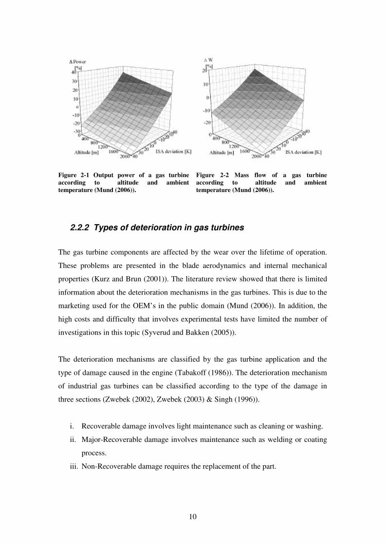
10
Figure 2-1 Output power of a gas turbine
according to altitude and ambient
temperature (Mund (2006)).
Figure 2-2 Mass flow of a gas turbine
according to altitude and ambient
temperature (Mund (2006)).
2.2.2 Types of deterioration in gas turbines
The gas turbine components are affected by the wear over the lifetime of operation.
These problems are presented in the blade aerodynamics and internal mechanical
properties (Kurz and Brun (2001)). The literature review showed that there is limited
information about the deterioration mechanisms in the gas turbines. This is due to the
marketing used for the OEM’s in the public domain (Mund (2006)). In addition, the
high costs and difficulty that involves experimental tests have limited the number of
investigations in this topic (Syverud and Bakken (2005)).
The deterioration mechanisms are classified by the gas turbine application and the
type of damage caused in the engine (Tabakoff (1986)). The deterioration mechanism
of industrial gas turbines can be classified according to the type of the damage in
three sections (Zwebek (2002), Zwebek (2003) & Singh (1996)).
i. Recoverable damage involves light maintenance such as cleaning or washing.
ii. Major-Recoverable damage involves maintenance such as welding or coating
process.
iii. Non-Recoverable damage requires the replacement of the part.
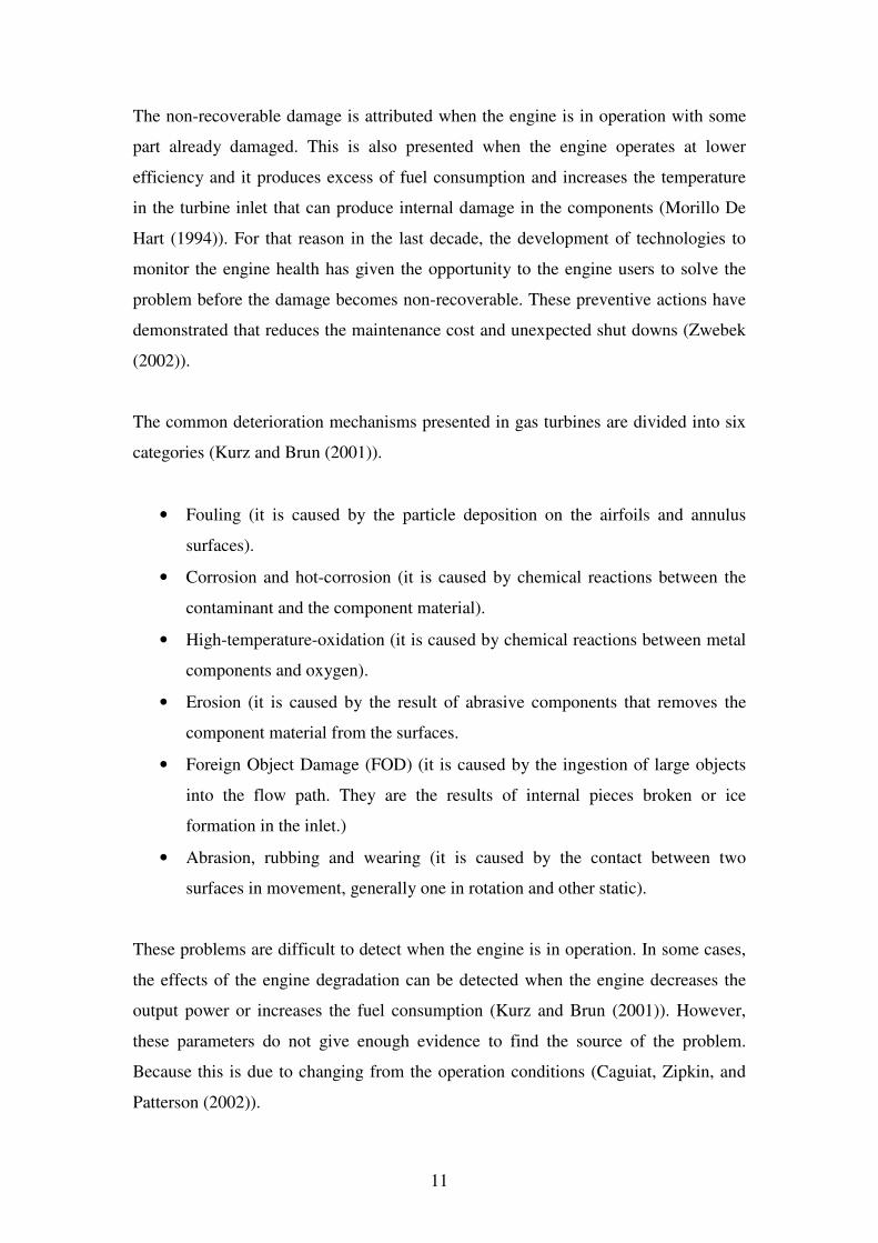
11
The non-recoverable damage is attributed when the engine is in operation with some
part already damaged. This is also presented when the engine operates at lower
efficiency and it produces excess of fuel consumption and increases the temperature
in the turbine inlet that can produce internal damage in the components (Morillo De
Hart (1994)). For that reason in the last decade, the development of technologies to
monitor the engine health has given the opportunity to the engine users to solve the
problem before the damage becomes non-recoverable. These preventive actions have
demonstrated that reduces the maintenance cost and unexpected shut downs (Zwebek
(2002)).
The common deterioration mechanisms presented in gas turbines are divided into six
categories (Kurz and Brun (2001)).
• Fouling (it is caused by the particle deposition on the airfoils and annulus
surfaces).
• Corrosion and hot-corrosion (it is caused by chemical reactions between the
contaminant and the component material).
• High-temperature-oxidation (it is caused by chemical reactions between metal
components and oxygen).
• Erosion (it is caused by the result of abrasive components that removes the
component material from the surfaces.
• Foreign Object Damage (FOD) (it is caused by the ingestion of large objects
into the flow path. They are the results of internal pieces broken or ice
formation in the inlet.)
• Abrasion, rubbing and wearing (it is caused by the contact between two
surfaces in movement, generally one in rotation and other static).
These problems are difficult to detect when the engine is in operation. In some cases,
the effects of the engine degradation can be detected when the engine decreases the
output power or increases the fuel consumption (Kurz and Brun (2001)). However,
these parameters do not give enough evidence to find the source of the problem.
Because this is due to changing from the operation conditions (Caguiat, Zipkin, and
Patterson (2002)).
12
2.2.3 Compressor degradation
Compressor fouling is produced due to the ingestion of dust mixed with the air. This
mechanism decreases the compressor isentropic efficiency. Fouling and erosion have
been demonstrated to affect the thermal efficiency and output power of the engine
(Zwebek (1993)). The deposition of the particles in critical areas can change the
geometry of the airfoils and then the flow condition is modified (Lakshminarasimha,
Boyce, and Meher-Homji (1994)). In addition, the accumulation of dust reduces the
tip clearance and increases the roughness of the surface roughness (Kurz and Brun
(2001)). These changes in the blades affect the compressor delivery pressure (CDP)
and reduce the mass flow.
Howell and Calvert (1978) & Aker and Saravanamuttoo (1989) calculated the impact
of degradation mechanisms in the compressor performance based on the output power
of the engine. Gulen, Griffin, and Paolucci (2002) reported that fouling decreased by
5% the output power due to mass flow reduction.
2.2.4 Combustion chamber degradation
The combustion chamber is one of the sections with a low level of degradation. The
operation time of the combustion chamber has an irrelevant effect to degrade this
section (Diakunchak (1991)). However, small variations in the combustion process
such as increment of the fuel ratio can affect the components from the turbine section.
For that reason, it is necessary to control the process of combustion. In addition, an
incorrect combustion can produce ash that is deposited in the fuel injectors. This
problem produces fluctuations in the flame and high local temperatures. The alteration
in the temperature profiles increases the possibility of secondary flows, reduces the
turbine efficiency and damages the turbine blades (Kurz and Brun (2001)).
2.2.5 Turbine degradation
Erosion is a common problem present in this section that modifies the profile of the
blades. Fouling is also present in the turbine blades due to ash adhesion on the
surfaces (Zwebek (2002)). It has been demonstrated that fouling on the turbine blades
13
reduces the turbine isentropic efficiency by 1% and the output by 3.7% (Diakunchak
(1991)). As it was mentioned in the previous section, the high temperatures and
incomplete fuel burning affect the turbine section due to overheating. This effect is
responsible for hot corrosion that modifies the shape of the leading edge from the
blades (Kurz and Brun (2001).
2.2.6 Monitoring, simulation and diagnosis of gas turbines degradation
Due to the fuel prices crisis in the last decades, many gas turbine users have
introduced the use of technologies for monitoring the engine performance. The data
obtained from engine monitoring have estimated the deterioration of the gas turbine.
This information is used to schedule the preventive maintenance and to extend the
period of the optimal production (Williams (1981), Haq and Saravanamuttoo (1991)).
For example Pinelli (2002) reported a gas turbine model AVIO TG20 that reduced in
the first month 4.1% of the power production due to degradation. Similar result was
reported by Gulen, Griffin, and Paolucci (2002) where two single shaft gas turbines in
operation in CCGT reduced 5% the output power in the first month. Mund (2006)
mentioned that the single shaft configuration has a high sensitivity in the output
power when the aerodynamics of the flow changes. For that reason, it is necessary in
power plant applications the periodic maintenance in the engine (Zwebek (2003)).
The typical overall maintenance period for industrial engines is approximately
between 3000 to 4000 hours of operation. At the end of this period it is possible to
find that the engine has lost 20% of the production capacity (Zwebek (2002)).
In the last decade, the development of algorithms based on the engine monitoring has
created the possibility of detecting the location of the problem in the engine and
predict the failure. Gulen, Griffin, and Paolucci (2002)) presented a model* based on
the real time of monitoring the engine performance in order to predict the gas turbine
degradation. The model compares the parameters given by the manufacturer and the
values represented from deterioration factors.
* Equation that represents the engine at full load condition, for part load condition sees reference.
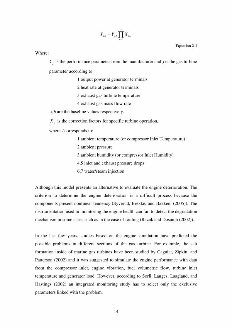
14
∏=
=7
1,,,
i
jibjxj XYY
Equation 2-1
Where:
jY is the performance parameter from the manufacturer and j is the gas turbine
parameter according to:
1 output power at generator terminals
2 heat rate at generator terminals
3 exhaust gas turbine temperature
4 exhaust gas mass flow rate
bx, are the baseline values respectively.
ijX is the correction factors for specific turbine operation,
where i corresponds to:
1 ambient temperature (or compressor Inlet Temperature)
2 ambient pressure
3 ambient humidity (or compressor Inlet Humidity)
4,5 inlet and exhaust pressure drops
6,7 water/steam injection
Although this model presents an alternative to evaluate the engine deterioration. The
criterion to determine the engine deterioration is a difficult process because the
components present nonlinear tendency (Syverud, Brekke, and Bakken, (2005)). The
instrumentation used in monitoring the engine health can fail to detect the degradation
mechanism in some cases such as in the case of fouling (Razak and Dosanjh (2002)).
In the last few years, studies based on the engine simulation have predicted the
possible problems in different sections of the gas turbine. For example, the salt
formation inside of marine gas turbines have been studied by Caguiat, Zipkin, and
Patterson (2002) and it was suggested to simulate the engine performance with data
from the compressor inlet, engine vibration, fuel volumetric flow, turbine inlet
temperature and generator load. However, according to Sorli, Langes, Laagland, and
Hastings (2002) an integrated monitoring study has to select only the exclusive
parameters linked with the problem.
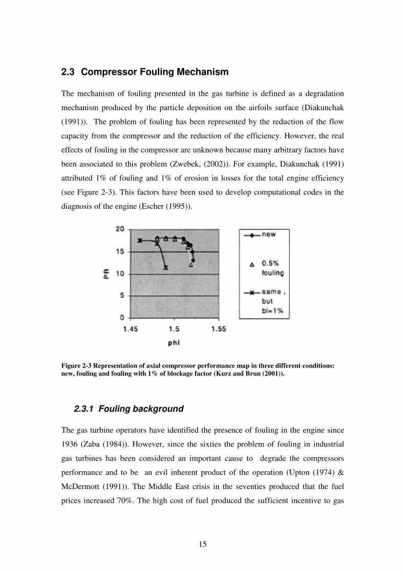
15
2.3 Compressor Fouling Mechanism
The mechanism of fouling presented in the gas turbine is defined as a degradation
mechanism produced by the particle deposition on the airfoils surface (Diakunchak
(1991)). The problem of fouling has been represented by the reduction of the flow
capacity from the compressor and the reduction of the efficiency. However, the real
effects of fouling in the compressor are unknown because many arbitrary factors have
been associated to this problem (Zwebek, (2002)). For example, Diakunchak (1991)
attributed 1% of fouling and 1% of erosion in losses for the total engine efficiency
(see Figure 2-3). This factors have been used to develop computational codes in the
diagnosis of the engine (Escher (1995)).
Figure 2-3 Representation of axial compressor performance map in three different conditions:
new, fouling and fouling with 1% of blockage factor (Kurz and Brun (2001)).
2.3.1 Fouling background
The gas turbine operators have identified the presence of fouling in the engine since
1936 (Zaba (1984)). However, since the sixties the problem of fouling in industrial
gas turbines has been considered an important cause to degrade the compressors
performance and to be an evil inherent product of the operation (Upton (1974) &
McDermott (1991)). The Middle East crisis in the seventies produced that the fuel
prices increased 70%. The high cost of fuel produced the sufficient incentive to gas

16
turbine operators to look for new technologies to abate the mechanism of degradation
to obtain optimal efficiencies for long periods (McDermott (1991)).
The studies in this area have demonstrated that the fouling mechanism represents
approximately 80% of the compressor losses. A reduction of 5% from the mass flow
can reduce 13% the output power and increase 5.5% the heat rate (Hoeft (1993) &
Mustafa (2006)). These losses represent millions of USD in power and fuel
consumption (Diakunchak (1991) & Mustafa (2006)).
Fouling is found in all engines due to the big quantities of air ingested. A typical gas
turbine in operation in a residential location ingests 1.5 kg of solid contaminants per
day (Zaba (1984)). For example, an engine of 7.5MW in an environment with
particles concentration of 1 ppm can ingest 5 kg of dust in a single day (Tabakoff
(1986)). This problem could turn worse if the engine operates in a very polluted
environment such as mining or oil field areas where the ingestion of foreign particles
can rise up to 39kg per day (Mustafa (2006)). It is necessary to pay careful attention
to the inlet of the engine, because the ingestion of high quantities of particles reduces
also the engine life (Osborne (1977)). In general, the industrial gas turbines are
installed with inlet filters that stop the pass of particles (Tarabrin, Bodrov,
Schurovsky, and Stalder (1996)). The size of particles stopped by the filters can be in
the range of µ m (Meher-Homji and Cyrus B, (1990)).
The selection of the filtration system has to be made and selected according to the
environment conditions (Mustafa (2006)). In modern power plants, the filtration
system involves different stages of filtration that consist in cylindrical and conical
arrangements of synthetic media filters (Huff & Puff* systems). For example,
filtration for industrial engines require efficiency of 99.5% for particle retention in the
range of 1-3µm (Boyce and Gonzalez (2005)). In the case of marine or off shore
applications, the filtration system has to stop the ingestion of chemical vapours and
salt† (Orsach, Kazcprzynski, Roemer, Scharschan, Caguiat, and McGroarty (2002)).
* Huff & Puff is a gas turbine filtration configuration to operate in positive or negative conditions of the flow. Source Donaldson Company GTS-102 rev6/05. † The typical salt-air concentration in a marine gas turbine after filtration is approximately of 0.01 ppm (Caguiat (2003)).
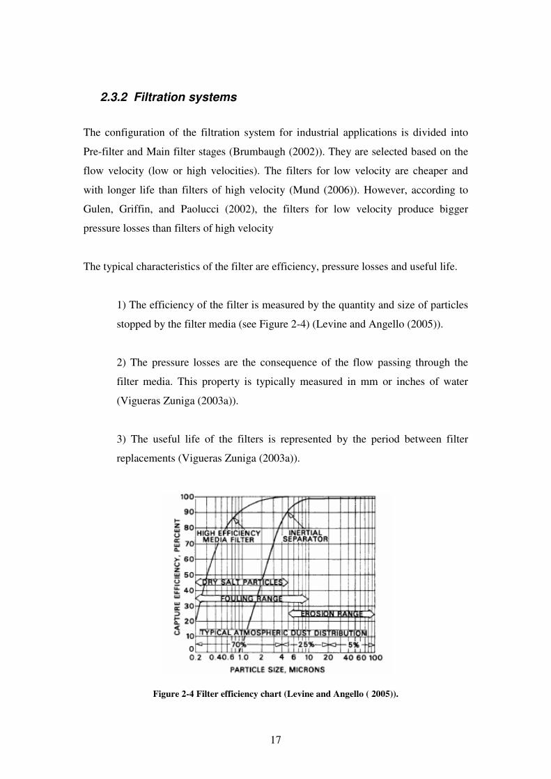
17
2.3.2 Filtration systems
The configuration of the filtration system for industrial applications is divided into
Pre-filter and Main filter stages (Brumbaugh (2002)). They are selected based on the
flow velocity (low or high velocities). The filters for low velocity are cheaper and
with longer life than filters of high velocity (Mund (2006)). However, according to
Gulen, Griffin, and Paolucci (2002), the filters for low velocity produce bigger
pressure losses than filters of high velocity
The typical characteristics of the filter are efficiency, pressure losses and useful life.
1) The efficiency of the filter is measured by the quantity and size of particles
stopped by the filter media (see Figure 2-4) (Levine and Angello (2005)).
2) The pressure losses are the consequence of the flow passing through the
filter media. This property is typically measured in mm or inches of water
(Vigueras Zuniga (2003a)).
3) The useful life of the filters is represented by the period between filter
replacements (Vigueras Zuniga (2003a)).
Figure 2-4 Filter efficiency chart (Levine and Angello ( 2005)).
18
The filter systems used in industrial applications are pulse-clean or static filters. The
pulse-clean system (self-cleaning filter) retains the particles on the filter surface. The
maintenance is automatic and consists of changing the filter orientation and passing a
secondary air stream through the filter. The particles are removed from the surface
and deposited outside of the inlet (Donaldson Company (2005)). Pulse-clean systems
have demonstrated 98% efficiency of retention in the particle size range of 3µm with
pressure losses of 4 inH2O (1000Pa) (Brumbaugh (2002)). The static filters are fixed
in static panels and the maintenance is manual. The advantage of these filters is the
long period of the useful life (Vigueras Zuniga (2003a)).
The Pre-filters stage consists of hoods, wraps and filters. Their job is to extend the life
of the main filters. The retention in this stage includes large foreign particles (birds,
seeds, leaves, airbone fibers, etc). The function of the inlet hoods is to avoid the
ingestion of rain or snow. The wraps is a plastic net with large spaces from the grill to
reduce the pressure losses at the same time that stop the inlet of big objects. The
filters located in this stage are static and with low efficiencies of filtration. The filter
media is an arrangement of polyester fibers randomly orientated to create an artificial
web (Vigueras Zuniga (2003a)).
The main stage of the filtration system provides a high efficiency of filtration:
retention of 95% in the arrange of 2µm particle size (Brumbaugh (2002)). They can
be pulse clean filter systems or static filter systems. The filter packing technique
combines different materials and properties. Special fibers are added to the filter
packing to retain corrosive particles such as salt or chemical vapours. In hardness
environments it is necessary to install a third filtration stage as a barrier to the salt
immigration from the main filters (Vigueras Zuniga (2003a) & Donaldson Company
(2005)). In naval applications, the third stage of filtration is used to stop the salt
migration with particle size filters of 13µm (Caguiat (2003)). The use of new fibers
have reduced the size of particle retention with acceptable pressure losses (Gahr,
Benson, Graham, Gogins, and Brown (2005) & Meher-Homji and Cyrus B (1990)).
The problems of filters in gas turbine applications are summarized as follows.
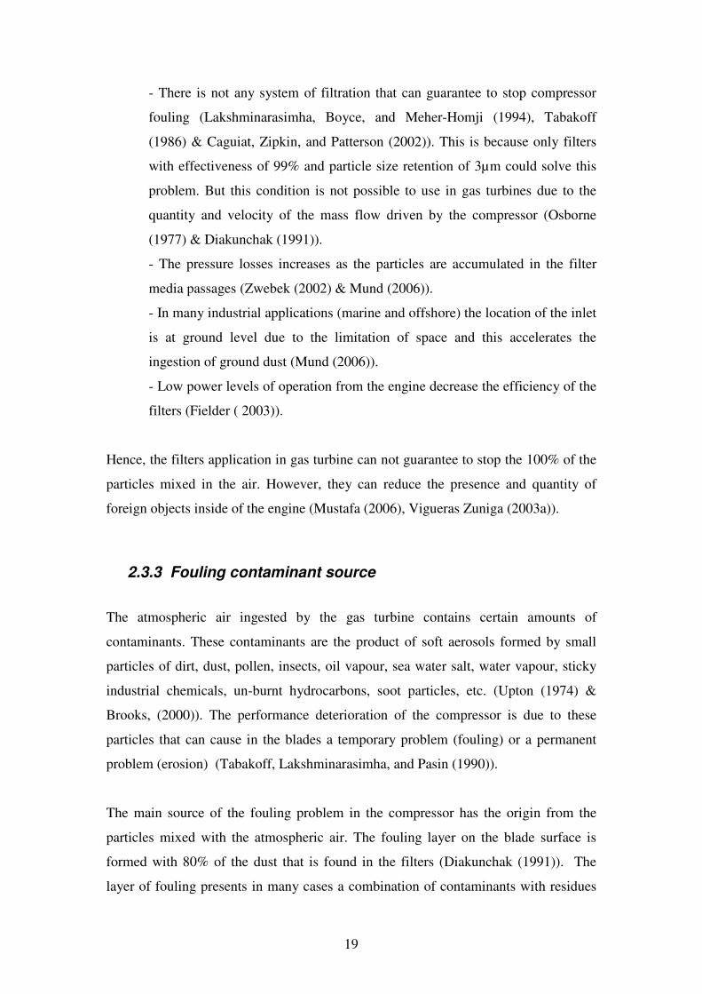
19
- There is not any system of filtration that can guarantee to stop compressor
fouling (Lakshminarasimha, Boyce, and Meher-Homji (1994), Tabakoff
(1986) & Caguiat, Zipkin, and Patterson (2002)). This is because only filters
with effectiveness of 99% and particle size retention of 3µm could solve this
problem. But this condition is not possible to use in gas turbines due to the
quantity and velocity of the mass flow driven by the compressor (Osborne
(1977) & Diakunchak (1991)).
- The pressure losses increases as the particles are accumulated in the filter
media passages (Zwebek (2002) & Mund (2006)).
- In many industrial applications (marine and offshore) the location of the inlet
is at ground level due to the limitation of space and this accelerates the
ingestion of ground dust (Mund (2006)).
- Low power levels of operation from the engine decrease the efficiency of the
filters (Fielder ( 2003)).
Hence, the filters application in gas turbine can not guarantee to stop the 100% of the
particles mixed in the air. However, they can reduce the presence and quantity of
foreign objects inside of the engine (Mustafa (2006), Vigueras Zuniga (2003a)).
2.3.3 Fouling contaminant source
The atmospheric air ingested by the gas turbine contains certain amounts of
contaminants. These contaminants are the product of soft aerosols formed by small
particles of dirt, dust, pollen, insects, oil vapour, sea water salt, water vapour, sticky
industrial chemicals, un-burnt hydrocarbons, soot particles, etc. (Upton (1974) &
Brooks, (2000)). The performance deterioration of the compressor is due to these
particles that can cause in the blades a temporary problem (fouling) or a permanent
problem (erosion) (Tabakoff, Lakshminarasimha, and Pasin (1990)).
The main source of the fouling problem in the compressor has the origin from the
particles mixed with the atmospheric air. The fouling layer on the blade surface is
formed with 80% of the dust that is found in the filters (Diakunchak (1991)). The
layer of fouling presents in many cases a combination of contaminants with residues
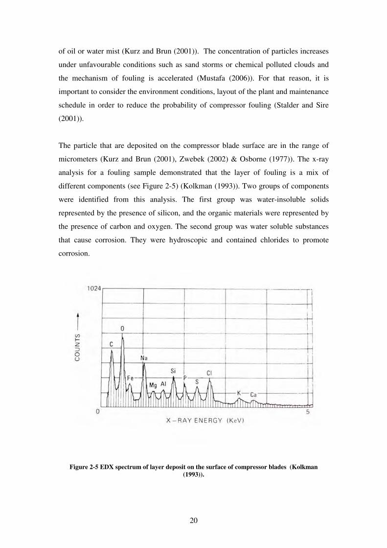
20
of oil or water mist (Kurz and Brun (2001)). The concentration of particles increases
under unfavourable conditions such as sand storms or chemical polluted clouds and
the mechanism of fouling is accelerated (Mustafa (2006)). For that reason, it is
important to consider the environment conditions, layout of the plant and maintenance
schedule in order to reduce the probability of compressor fouling (Stalder and Sire
(2001)).
The particle that are deposited on the compressor blade surface are in the range of
micrometers (Kurz and Brun (2001), Zwebek (2002) & Osborne (1977)). The x-ray
analysis for a fouling sample demonstrated that the layer of fouling is a mix of
different components (see Figure 2-5) (Kolkman (1993)). Two groups of components
were identified from this analysis. The first group was water-insoluble solids
represented by the presence of silicon, and the organic materials were represented by
the presence of carbon and oxygen. The second group was water soluble substances
that cause corrosion. They were hydroscopic and contained chlorides to promote
corrosion.
Figure 2-5 EDX spectrum of layer deposit on the surface of compressor blades (Kolkman
(1993)).
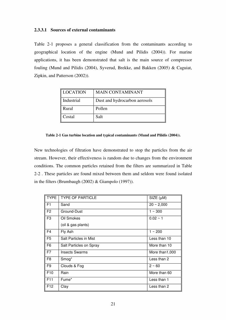
21
2.3.3.1 Sources of external contaminants
Table 2-1 proposes a general classification from the contaminants according to
geographical location of the engine (Mund and Pilidis (2004)). For marine
applications, it has been demonstrated that salt is the main source of compressor
fouling (Mund and Pilidis (2004), Syverud, Brekke, and Bakken (2005) & Caguiat,
Zipkin, and Patterson (2002)).
LOCATION MAIN CONTAMINANT
Industrial Dust and hydrocarbon aerosols
Rural Pollen
Costal Salt
Table 2-1 Gas turbine location and typical contaminants (Mund and Pilidis (2004)).
New technologies of filtration have demonstrated to stop the particles from the air
stream. However, their effectiveness is random due to changes from the environment
conditions. The common particles retained from the filters are summarized in Table
2-2 . These particles are found mixed between them and seldom were found isolated
in the filters (Brumbaugh (2002) & Giampolo (1997)).
TYPE TYPE OF PARTICLE SIZE (µM)
F1 Sand 20 ~ 2,000
F2 Ground-Dust 1 ~ 300
F3 Oil Smokes
(oil & gas plants)
0.02 ~ 1
F4 Fly Ash 1 ~ 200
F5 Salt Particles in Mist Less than 10
F6 Salt Particles on Spray More than 10
F7 Insects Swarms More than1,000
F8 Smog* Less than 2
F9 Clouds & Fog 2 ~ 60
F10 Rain More than 60
F11 Fume* Less than 1
F12 Clay Less than 2
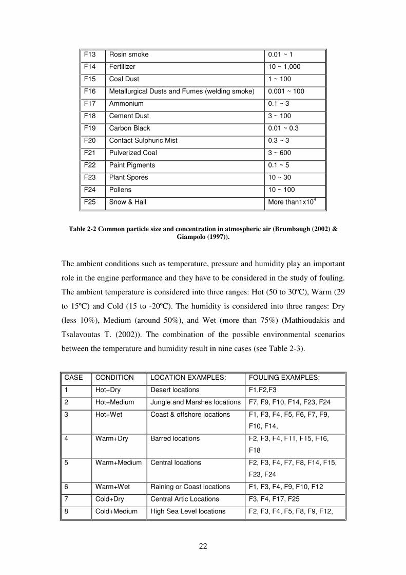
22
F13 Rosin smoke 0.01 ~ 1
F14 Fertilizer 10 ~ 1,000
F15 Coal Dust 1 ~ 100
F16 Metallurgical Dusts and Fumes (welding smoke) 0.001 ~ 100
F17 Ammonium 0.1 ~ 3
F18 Cement Dust 3 ~ 100
F19 Carbon Black 0.01 ~ 0.3
F20 Contact Sulphuric Mist 0.3 ~ 3
F21 Pulverized Coal 3 ~ 600
F22 Paint Pigments 0.1 ~ 5
F23 Plant Spores 10 ~ 30
F24 Pollens 10 ~ 100
F25 Snow & Hail More than1x104
Table 2-2 Common particle size and concentration in atmospheric air (Brumbaugh (2002) &
Giampolo (1997)).
The ambient conditions such as temperature, pressure and humidity play an important
role in the engine performance and they have to be considered in the study of fouling.
The ambient temperature is considered into three ranges: Hot (50 to 30ºC), Warm (29
to 15ºC) and Cold (15 to -20ºC). The humidity is considered into three ranges: Dry
(less 10%), Medium (around 50%), and Wet (more than 75%) (Mathioudakis and
Tsalavoutas T. (2002)). The combination of the possible environmental scenarios
between the temperature and humidity result in nine cases (see Table 2-3).
CASE CONDITION LOCATION EXAMPLES: FOULING EXAMPLES:
1 Hot+Dry Desert locations F1,F2,F3
2 Hot+Medium Jungle and Marshes locations F7, F9, F10, F14, F23, F24
3 Hot+Wet Coast & offshore locations F1, F3, F4, F5, F6, F7, F9,
F10, F14,
4 Warm+Dry Barred locations F2, F3, F4, F11, F15, F16,
F18
5 Warm+Medium Central locations F2, F3, F4, F7, F8, F14, F15,
F23, F24
6 Warm+Wet Raining or Coast locations F1, F3, F4, F9, F10, F12
7 Cold+Dry Central Artic Locations F3, F4, F17, F25
8 Cold+Medium High Sea Level locations F2, F3, F4, F5, F8, F9, F12,
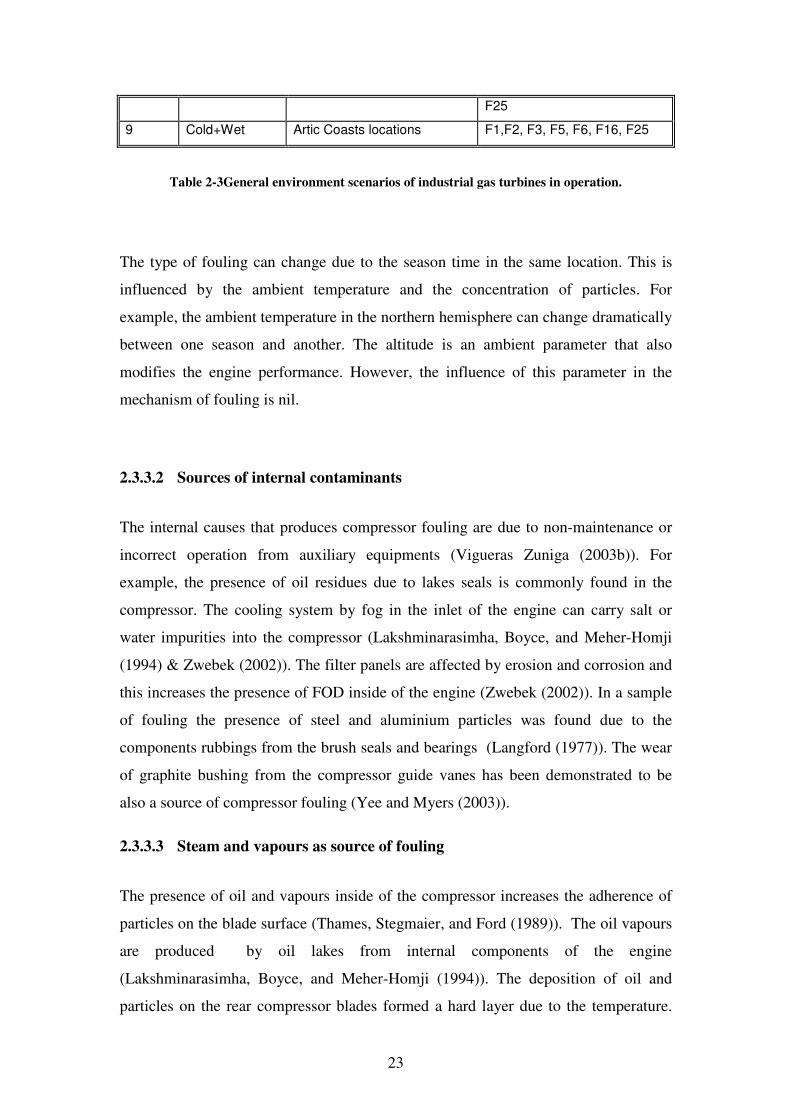
23
F25
9 Cold+Wet Artic Coasts locations F1,F2, F3, F5, F6, F16, F25
Table 2-3General environment scenarios of industrial gas turbines in operation.
The type of fouling can change due to the season time in the same location. This is
influenced by the ambient temperature and the concentration of particles. For
example, the ambient temperature in the northern hemisphere can change dramatically
between one season and another. The altitude is an ambient parameter that also
modifies the engine performance. However, the influence of this parameter in the
mechanism of fouling is nil.
2.3.3.2 Sources of internal contaminants
The internal causes that produces compressor fouling are due to non-maintenance or
incorrect operation from auxiliary equipments (Vigueras Zuniga (2003b)). For
example, the presence of oil residues due to lakes seals is commonly found in the
compressor. The cooling system by fog in the inlet of the engine can carry salt or
water impurities into the compressor (Lakshminarasimha, Boyce, and Meher-Homji
(1994) & Zwebek (2002)). The filter panels are affected by erosion and corrosion and
this increases the presence of FOD inside of the engine (Zwebek (2002)). In a sample
of fouling the presence of steel and aluminium particles was found due to the
components rubbings from the brush seals and bearings (Langford (1977)). The wear
of graphite bushing from the compressor guide vanes has been demonstrated to be
also a source of compressor fouling (Yee and Myers (2003)).
2.3.3.3 Steam and vapours as source of fouling
The presence of oil and vapours inside of the compressor increases the adherence of
particles on the blade surface (Thames, Stegmaier, and Ford (1989)). The oil vapours
are produced by oil lakes from internal components of the engine
(Lakshminarasimha, Boyce, and Meher-Homji (1994)). The deposition of oil and
particles on the rear compressor blades formed a hard layer due to the temperature.
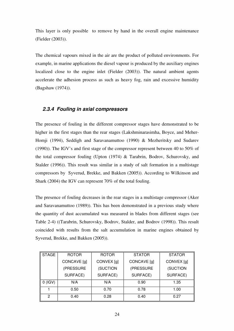
24
This layer is only possible to remove by hand in the overall engine maintenance
(Fielder (2003)).
The chemical vapours mixed in the air are the product of polluted environments. For
example, in marine applications the diesel vapour is produced by the auxiliary engines
localized close to the engine inlet (Fielder (2003)). The natural ambient agents
accelerate the adhesion process as such as heavy fog, rain and excessive humidity
(Bagshaw (1974)).
2.3.4 Fouling in axial compressors
The presence of fouling in the different compressor stages have demonstrated to be
higher in the first stages than the rear stages (Lakshminarasimha, Boyce, and Meher-
Homji (1994), Seddigh and Saravanamuttoo (1990) & Mezheritsky and Sudarev
(1990)). The IGV’s and first stage of the compressor represent between 40 to 50% of
the total compressor fouling (Upton (1974) & Tarabrin, Bodrov, Schurovsky, and
Stalder (1996)). This result was similar in a study of salt formation in a multistage
compressors by Syverud, Brekke, and Bakken (2005)). According to Wilkinson and
Shark (2004) the IGV can represent 70% of the total fouling.
The presence of fouling decreases in the rear stages in a multistage compressor (Aker
and Saravanamuttoo (1989)). This has been demonstrated in a previous study where
the quantity of dust accumulated was measured in blades from different stages (see
Table 2-4) ((Tarabrin, Schurovsky, Bodrov, Stalder, and Bodrov (1998)). This result
coincided with results from the salt accumulation in marine engines obtained by
Syverud, Brekke, and Bakken (2005)).
STAGE ROTOR
CONCAVE [g]
(PRESSURE
SURFACE)
ROTOR
CONVEX [g]
(SUCTION
SURFACE)
STATOR
CONCAVE [g]
(PRESSURE
SURFACE)
STATOR
CONVEX [g]
(SUCTION
SURFACE)
0 (IGV) N/A N/A 0.90 1.35
1 0.50 0.70 0.78 1.00
2 0.40 0.28 0.40 0.27
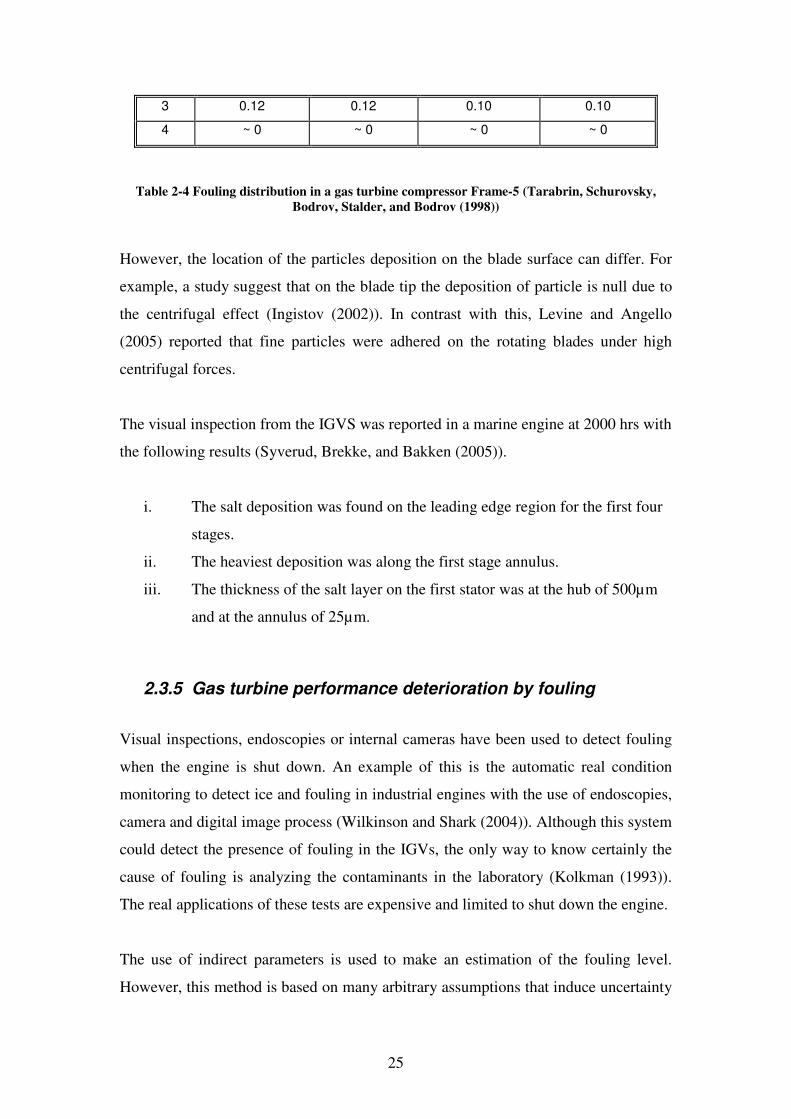
25
3 0.12 0.12 0.10 0.10
4 ~ 0 ~ 0 ~ 0 ~ 0
Table 2-4 Fouling distribution in a gas turbine compressor Frame-5 (Tarabrin, Schurovsky,
Bodrov, Stalder, and Bodrov (1998))
However, the location of the particles deposition on the blade surface can differ. For
example, a study suggest that on the blade tip the deposition of particle is null due to
the centrifugal effect (Ingistov (2002)). In contrast with this, Levine and Angello
(2005) reported that fine particles were adhered on the rotating blades under high
centrifugal forces.
The visual inspection from the IGVS was reported in a marine engine at 2000 hrs with
the following results (Syverud, Brekke, and Bakken (2005)).
i. The salt deposition was found on the leading edge region for the first four
stages.
ii. The heaviest deposition was along the first stage annulus.
iii. The thickness of the salt layer on the first stator was at the hub of 500µm
and at the annulus of 25µm.
2.3.5 Gas turbine performance deterioration by fouling
Visual inspections, endoscopies or internal cameras have been used to detect fouling
when the engine is shut down. An example of this is the automatic real condition
monitoring to detect ice and fouling in industrial engines with the use of endoscopies,
camera and digital image process (Wilkinson and Shark (2004)). Although this system
could detect the presence of fouling in the IGVs, the only way to know certainly the
cause of fouling is analyzing the contaminants in the laboratory (Kolkman (1993)).
The real applications of these tests are expensive and limited to shut down the engine.
The use of indirect parameters is used to make an estimation of the fouling level.
However, this method is based on many arbitrary assumptions that induce uncertainty
26
in the results, because, in the real application, the turbine entry temperature (TET) is
estimated from the turbine output power (Saravanamuttoo and Lakshminarasimha
(1985)). According to Haq and Saravanamuttoo (1991) small engines can present a
fast degradation because fouling reduces the compressor performance and is
represented by increases the TET. However, according to Kurz and Brun (2001) this
condition does not represent the average value of TET and represents the temperature
of a local flame. The engine size is a topic of discussion because some reports agree
that small engines are more susceptible to degradation as (Tarabrin, Schurovsky,
Bodrov, Stalder, and Bodrov (1998)) and another argue exactly the opposite as (Aker
and Saravanamuttoo (1989) & Haq and Saravanamuttoo (1991)).
The output power of the engine is used for many gas turbine users to predict the
fouling. However, this method does not always represent the real situation due that
the automatic control of the engine adjusts the internal components. This problem is
illustrate in the study of an engine that was re-adjusted after several hours of operation
(Kurz and Brun (2001)). After the engine was re-adjusted, the TET recovered the
original value but the power decreased 2.5%. It was then necessary to adjust the
engine by increasing the heat rate to 1.2% to obtain the original power. In this case,
the deterioration was evident and non-recoverable. This demonstrates that the engine
configuration plays an important role in the deterioration of the performance.
In the case of the compressor configuration, fouling has a higher impact in axial
compressors than in centrifugal compressors (Meher-Homji and Cyrus B (1990) &
Seddigh and Saravanamuttoo (1990)). The map of the axial compressor shows the
reduction of the surge margin due to fouling (Diakunchak (1991) & Seddigh and
Saravanamuttoo (1990)). The speed of the engine also could hide the fouling effect in
gas turbines. This is because the movement from the design point represented in the
compressor map could be easy confused with a different compressor line of operation
(Seddigh and Saravanamuttoo (1990)). The case is illustrated when the design point
of the compressor is located in a higher shaft speed point and lower efficiency. When
compressor fouling occurs, the compressor efficiency increases due to the reduction
of the shaft speed and then effect of fouling is difficult to detect (Kurz and Brun
(2001)).
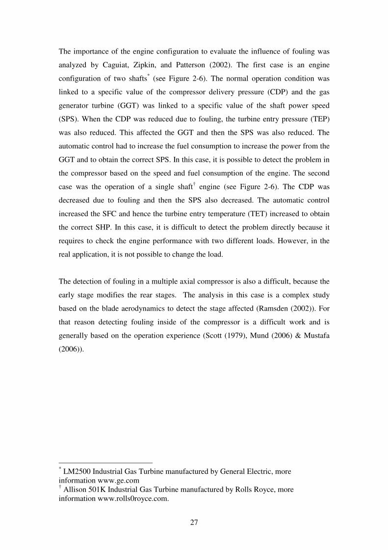
27
The importance of the engine configuration to evaluate the influence of fouling was
analyzed by Caguiat, Zipkin, and Patterson (2002). The first case is an engine
configuration of two shafts* (see Figure 2-6). The normal operation condition was
linked to a specific value of the compressor delivery pressure (CDP) and the gas
generator turbine (GGT) was linked to a specific value of the shaft power speed
(SPS). When the CDP was reduced due to fouling, the turbine entry pressure (TEP)
was also reduced. This affected the GGT and then the SPS was also reduced. The
automatic control had to increase the fuel consumption to increase the power from the
GGT and to obtain the correct SPS. In this case, it is possible to detect the problem in
the compressor based on the speed and fuel consumption of the engine. The second
case was the operation of a single shaft† engine (see Figure 2-6). The CDP was
decreased due to fouling and then the SPS also decreased. The automatic control
increased the SFC and hence the turbine entry temperature (TET) increased to obtain
the correct SHP. In this case, it is difficult to detect the problem directly because it
requires to check the engine performance with two different loads. However, in the
real application, it is not possible to change the load.
The detection of fouling in a multiple axial compressor is also a difficult, because the
early stage modifies the rear stages. The analysis in this case is a complex study
based on the blade aerodynamics to detect the stage affected (Ramsden (2002)). For
that reason detecting fouling inside of the compressor is a difficult work and is
generally based on the operation experience (Scott (1979), Mund (2006) & Mustafa
(2006)).
* LM2500 Industrial Gas Turbine manufactured by General Electric, more information www.ge.com † Allison 501K Industrial Gas Turbine manufactured by Rolls Royce, more information www.rolls0royce.com.
28
Figure 2-6 Gas turbine configuration: two-shafts configuration (left), single-shaft configuration
(right).
2.3.6 Surface roughness change and aerodynamic consequences in blades
The major contribution of fouling to decrease the efficiency and pressure ratio in axial
compressor is due to changes from the blade geometry (roughness and thickness of
the surface) (Mezheritsky and Sudarev, (1990) & Upton (1974)). The changes on the
surface roughness increase the friction with the air and affect the compression process
(Zwebek (2002)). The particle deposition reduces the cross-area section and the mass
flow is reduced by this effect. This modifies the pressure ratio and compressor
efficiency (Tabakoff, Lakshminarasimha, and Pasin (1990)). The increment of
roughness increases the friction losses that produces an early transition in the
boundary layer (laminar to turbulent) that is transmitted in the compressor
performance as losses (Kurz and Brun (2001)). Also, the particles tend to adhere
easily on rougher surfaces due to the frictional forces (Caguiat, Zipkin, and Patterson
(2002)).
The change of the surface roughness due to blade erosion has demonstrated that
affects the engine performance and increases the fuel consumption. According to
Lakshminarasimha, Boyce, and Meher-Homji (1994) if the surface roughness
increases from 55 to 120µm the fuel consumption also increased in 0.13%. Kurz and
Brun (2001) reported an increment of the surface roughness after a long time of
operation, the rotor blades increased from 4µm to 6.0µm and the stator blades to
Compressor Gas Generator Turbine
Power Turbine
Power Electrical Generator
Chamber Combustion
Shaft Power Turbine
Shaft Gas Generator Turbine
Compressor
Power Turbine
Power Electrical Generator
Chamber Combustion
Shaft Power Turbine
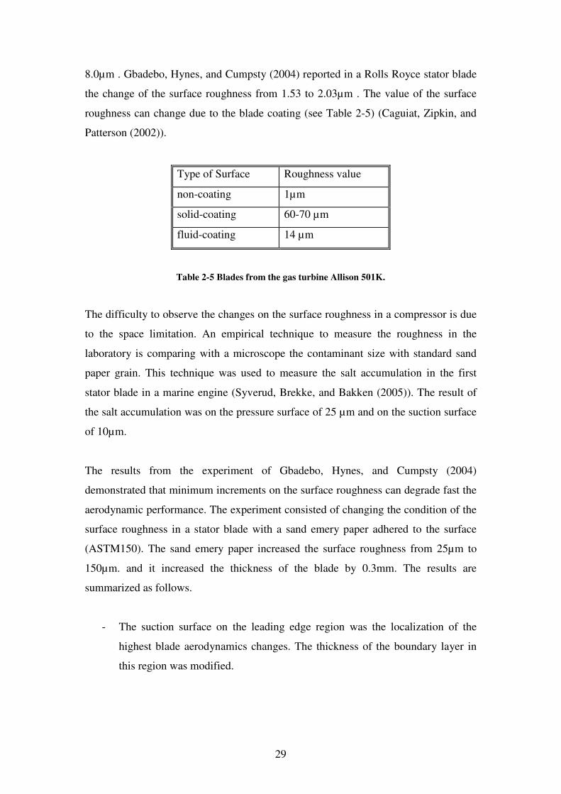
29
8.0µm . Gbadebo, Hynes, and Cumpsty (2004) reported in a Rolls Royce stator blade
the change of the surface roughness from 1.53 to 2.03µm . The value of the surface
roughness can change due to the blade coating (see Table 2-5) (Caguiat, Zipkin, and
Patterson (2002)).
Type of Surface Roughness value
non-coating 1µm
solid-coating 60-70 µm
fluid-coating 14 µm
Table 2-5 Blades from the gas turbine Allison 501K.
The difficulty to observe the changes on the surface roughness in a compressor is due
to the space limitation. An empirical technique to measure the roughness in the
laboratory is comparing with a microscope the contaminant size with standard sand
paper grain. This technique was used to measure the salt accumulation in the first
stator blade in a marine engine (Syverud, Brekke, and Bakken (2005)). The result of
the salt accumulation was on the pressure surface of 25 µm and on the suction surface
of 10µm.
The results from the experiment of Gbadebo, Hynes, and Cumpsty (2004)
demonstrated that minimum increments on the surface roughness can degrade fast the
aerodynamic performance. The experiment consisted of changing the condition of the
surface roughness in a stator blade with a sand emery paper adhered to the surface
(ASTM150). The sand emery paper increased the surface roughness from 25µm to
150µm. and it increased the thickness of the blade by 0.3mm. The results are
summarized as follows.
- The suction surface on the leading edge region was the localization of the
highest blade aerodynamics changes. The thickness of the boundary layer in
this region was modified.
30
- The major effect for three-dimensional separation was due to the increment of
the surface roughness in the hub of the stator blade. This effect was observed
on the suction surface close to the leading region.
- The numerical analysis demonstrated that the skin-friction coefficient
produced turbulent flows.
Similar to this result, Levine and Angello (2005) demonstrated in a numerical study
that increasing the surface roughness changed the thickness of the boundary layer
around the blade.
2.3.6.1 Boundary layer
The early separation from the boundary layer produces changes in the exit angle of
the blade and consequently affects the following stage (Ramsden (2002)). Small
changes from the airfoil shape produces changes in the inlet and incident angles from
the blades and reduces the airfoil throat opening (Diakunchak (1991)). According to
Caguiat, Zipkin, and Patterson (2002), the deposition of the particle can change the
effective angle of attack in each blade and produce the compressor stall. However,
Syverud, Brekke, and Bakken (2005) mentioned that the increment of the surface
roughness does not produce a significant change in the inlet angle or outlet angle.
The drag and thickness of the boundary layer are functions of the Reynolds number. If
the boundary layer tends to be laminar the drag and energy are reduced and opposite
to this result, it is when the boundary layer tends to be turbulent (Barlow, Rae, and
Pope (1999)). The transition point is produced when the boundary layer changes from
laminar to turbulence. This is a three dimensional phenomenon which occurs where
the laminar and turbulent flows coexist and it can be produced by natural process, for
a bypass or flow separation (Mayle (1991)). However, the two dimensional study for
the transition point in turbomachinery application is used in theoretical investigations
(Gbadebo, Hynes, and Cumpsty (2004) & Mayle (1991)). The effect of flow
separation transition can be consulted in the following reference Hobson, Hansen,
Schnorenberg, and Grove (2001).
31
The transition between laminar to turbulent can occur with any disturbance in the
flow around the blade (Mayle (1991)). For example, an imperfection from the smooth
surface can generate fluctuations in the flow that when it is amplified can produce:
- Turbulence due to formation of spots
- Bubbles on surfaces, when the flow is separated and reattached to the surface
The smooth surface of the blade produces forces that send backward the transition
point. This condition is produced when the surface roughness increases and then the
transition point is moved forward. In this case, the thickness of the boundary layer is
modified and produces two effects (Meher-Homji and Bromley (2004)).
i. The blade drag increases.
ii. The skin friction increases.
The study of Zaba (1984) demonstrated that due to blade coating the thickness of it
increases in 0.1mm. This can reduce the mass flow by 10% and the compressor
efficiency by 5%.
2.3.6.2 Surge margin
Fouling affects the airflow conditions due to the change of the velocity angle that
decreases the efficiency and the stall region margin from the compressor
(Saravanamuttoo and Lakshminarasimha (1985), Langford (1977) & Ramsden
(2002)). This reduction is due to the increment of the surface roughness that changes
the boundary layer thickness and reduces the aerodynamic properties from the blade
(Kurz and Brun (2001)). This change is represented in a compressor map when the
operation point is moving close to the surge line (Zwebek (1993), Saravanamuttoo
and Lakshminarasimha (1985), Olhovsky (1985) & Meher-Homji and Cyrus B
(1990)). According to Mustafa (2006) the condition of operation close to the surge
line is a dangerous situation for the compressor.
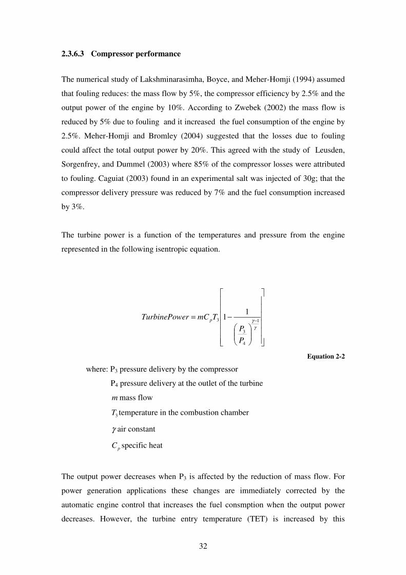
32
2.3.6.3 Compressor performance
The numerical study of Lakshminarasimha, Boyce, and Meher-Homji (1994) assumed
that fouling reduces: the mass flow by 5%, the compressor efficiency by 2.5% and the
output power of the engine by 10%. According to Zwebek (2002) the mass flow is
reduced by 5% due to fouling and it increased the fuel consumption of the engine by
2.5%. Meher-Homji and Bromley (2004) suggested that the losses due to fouling
could affect the total output power by 20%. This agreed with the study of Leusden,
Sorgenfrey, and Dummel (2003) where 85% of the compressor losses were attributed
to fouling. Caguiat (2003) found in an experimental salt was injected of 30g; that the
compressor delivery pressure was reduced by 7% and the fuel consumption increased
by 3%.
The turbine power is a function of the temperatures and pressure from the engine
represented in the following isentropic equation.
−=−
γ
γ 1
4
3
3
11
P
P
TmCerTurbinePow p
Equation 2-2
where: P3 pressure delivery by the compressor
P4 pressure delivery at the outlet of the turbine
m mass flow
3T temperature in the combustion chamber
γ air constant
pC specific heat
The output power decreases when P3 is affected by the reduction of mass flow. For
power generation applications these changes are immediately corrected by the
automatic engine control that increases the fuel consmption when the output power
decreases. However, the turbine entry temperature (TET) is increased by this
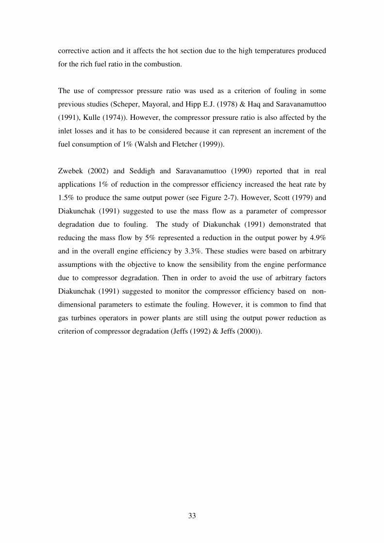
33
corrective action and it affects the hot section due to the high temperatures produced
for the rich fuel ratio in the combustion.
The use of compressor pressure ratio was used as a criterion of fouling in some
previous studies (Scheper, Mayoral, and Hipp E.J. (1978) & Haq and Saravanamuttoo
(1991), Kulle (1974)). However, the compressor pressure ratio is also affected by the
inlet losses and it has to be considered because it can represent an increment of the
fuel consumption of 1% (Walsh and Fletcher (1999)).
Zwebek (2002) and Seddigh and Saravanamuttoo (1990) reported that in real
applications 1% of reduction in the compressor efficiency increased the heat rate by
1.5% to produce the same output power (see Figure 2-7). However, Scott (1979) and
Diakunchak (1991) suggested to use the mass flow as a parameter of compressor
degradation due to fouling. The study of Diakunchak (1991) demonstrated that
reducing the mass flow by 5% represented a reduction in the output power by 4.9%
and in the overall engine efficiency by 3.3%. These studies were based on arbitrary
assumptions with the objective to know the sensibility from the engine performance
due to compressor degradation. Then in order to avoid the use of arbitrary factors
Diakunchak (1991) suggested to monitor the compressor efficiency based on non-
dimensional parameters to estimate the fouling. However, it is common to find that
gas turbines operators in power plants are still using the output power reduction as
criterion of compressor degradation (Jeffs (1992) & Jeffs (2000)).
34
Figure 2-7 Gas turbine efficiency based on deterioration in specific sections (Zwebek (2002))
2.3.6.4 Emissions
The environmental regulations ensure that the emission of gasses has to be controlled.
In this case fouling has an influence in the increment of the fuel consumption that
produces rich mixes* ((Boyce and Gonzalez, 2005)). This condition of excess of fuel
in the mix causes the production of NOx due to the high local temperatures produced
during the combustion ((Singh (2002)).
2.3.6.5 Mechanical problems
According to Zwebek (2002) fouling can produce separation of the boundary layer
that results in unexpected pressures on the blade surface. These conditions can
produce vibration and noise. Also, the changes of the exit blade angles due to fouling
can produce vibration Ramsden (2002). An excessive deposition of particles on the
airfoil surfaces reduces the cross section of the flow passage and it is possible to have
conditions of flow choke. Orsach, Kazcprzynski, Roemer, Scharschan, Caguiat, and
McGroarty (2002) suggested that compressor fouling evidently increases the * Rich mixes in the combustion process are produced when the fuel ratio increased respect the quantity of air (Singh (2002)).
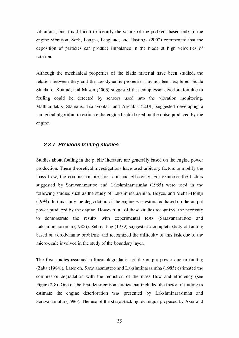
35
vibrations, but it is difficult to identify the source of the problem based only in the
engine vibration. Sorli, Langes, Laagland, and Hastings (2002) commented that the
deposition of particles can produce imbalance in the blade at high velocities of
rotation.
Although the mechanical properties of the blade material have been studied, the
relation between they and the aerodynamic properties has not been explored. Scala
Sinclaire, Konrad, and Mason (2003) suggested that compressor deterioration due to
fouling could be detected by sensors used into the vibration monitoring.
Mathioudakis, Stamatis, Tsalavoutas, and Aretakis (2001) suggested developing a
numerical algorithm to estimate the engine health based on the noise produced by the
engine.
2.3.7 Previous fouling studies
Studies about fouling in the public literature are generally based on the engine power
production. These theoretical investigations have used arbitrary factors to modify the
mass flow, the compressor pressure ratio and efficiency. For example, the factors
suggested by Saravanamuttoo and Lakshminarasimha (1985) were used in the
following studies such as the study of Lakshminarasimha, Boyce, and Meher-Homji
(1994). In this study the degradation of the engine was estimated based on the output
power produced by the engine. However, all of these studies recognized the necessity
to demonstrate the results with experimental tests (Saravanamuttoo and
Lakshminarasimha (1985)). Schlichting (1979) suggested a complete study of fouling
based on aerodynamic problems and recognized the difficulty of this task due to the
micro-scale involved in the study of the boundary layer.
The first studies assumed a linear degradation of the output power due to fouling
(Zaba (1984)). Later on, Saravanamuttoo and Lakshminarasimha (1985) estimated the
compressor degradation with the reduction of the mass flow and efficiency (see
Figure 2-8). One of the first deterioration studies that included the factor of fouling to
estimate the engine deterioration was presented by Lakshminarasimha and
Saravanamutto (1986). The use of the stage stacking technique proposed by Aker and
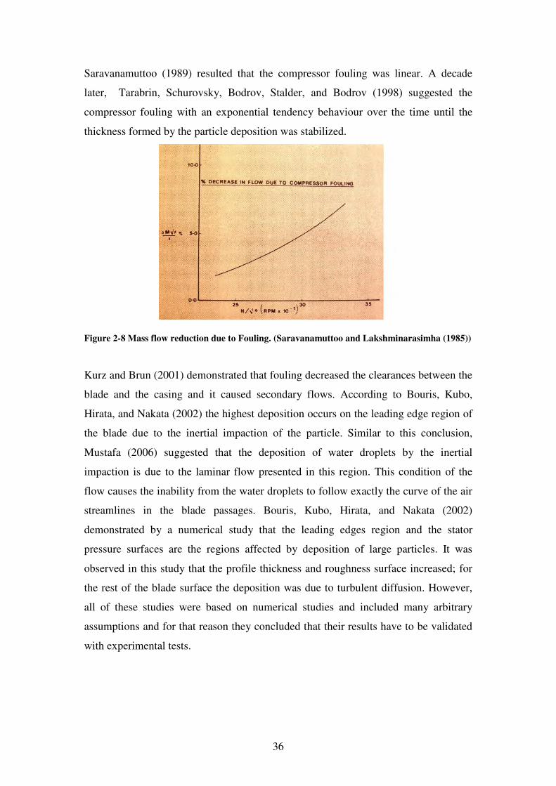
36
Saravanamuttoo (1989) resulted that the compressor fouling was linear. A decade
later, Tarabrin, Schurovsky, Bodrov, Stalder, and Bodrov (1998) suggested the
compressor fouling with an exponential tendency behaviour over the time until the
thickness formed by the particle deposition was stabilized.
Figure 2-8 Mass flow reduction due to Fouling. (Saravanamuttoo and Lakshminarasimha (1985))
Kurz and Brun (2001) demonstrated that fouling decreased the clearances between the
blade and the casing and it caused secondary flows. According to Bouris, Kubo,
Hirata, and Nakata (2002) the highest deposition occurs on the leading edge region of
the blade due to the inertial impaction of the particle. Similar to this conclusion,
Mustafa (2006) suggested that the deposition of water droplets by the inertial
impaction is due to the laminar flow presented in this region. This condition of the
flow causes the inability from the water droplets to follow exactly the curve of the air
streamlines in the blade passages. Bouris, Kubo, Hirata, and Nakata (2002)
demonstrated by a numerical study that the leading edges region and the stator
pressure surfaces are the regions affected by deposition of large particles. It was
observed in this study that the profile thickness and roughness surface increased; for
the rest of the blade surface the deposition was due to turbulent diffusion. However,
all of these studies were based on numerical studies and included many arbitrary
assumptions and for that reason they concluded that their results have to be validated
with experimental tests.
37
2.4 Compressor Washing
The maintenance of a gas turbine plays an important role for optimal performance.
For many years, compressor washing operated when the gas turbine was shut down
for overall maintenance (inspection, replacement of components and cleaning service)
(Vigueras Zuniga (2003b)). The first abrasive materials used for cleaning the
compressor were nutshells, rice and synthetic resin particles introduced at high
velocities into the compressor working off line. This method of compressor washing
resulted quick and effective, however this produced erosion in the blade (Mund and
Pilidis (2004)).
The method of cleaning by soft erosion was replaced by the use of water injection.
The injection of water from the inlet followed the same technique used to boost the
power in aero-engines with the use of water injection into the compressor (Mund
(2006)). Water injection includes characteristics as injection of fluid, droplet impact
on blades, fluid radial displacement, droplet size, re-ingestion and heat transfer
(Murthy, Ehresman, and Haykin (1986) & Mund and Pilidis (2004)). The first patents
of water injection into the compressor were presented in the seventies. The patent by
Freid and Tapparo (1971) included a spray system of four nozzles injecting parallel to
the air stream. A few years later Mansson (1975) patented a system to spray water
with low speeds in order to penetrate until the rear stages (Mund (2006)).
During the eighties the improvements in the aerodynamic airfoil geometry obligated
to reduce the level of erosion allowed in the blades (Brittain (1983)). For that reason,
during this decade the first studies of automatic and controlled systems of compressor
washing were tested in power plants (Mund (2006)). The use of demineralised water
to wash the compressor demonstrated non erosion on the blades and was adopted for
compressor washing with a combination of clean liquids (water-detergent or water-
petroleum solvent) (Boyce, Bowman, Meher-Homji, and Focke (1985)). In 1986 a
patent to clean the gas turbine at full speed was presented, this result was considerable
improved in the engine performance (McDermott (1991) and Mund (2006)). The
results from the study of Thames, Stegmaier, and Ford (1989) demonstrated the
possibility to wash the compressor during normal operation, and this process was
called compressor washing on line. Improvements in the compressor washing on line
38
continued during the nineties. During this decade the gas turbine users found interest
in this technology to improve the engine performance (McDermott (1991)). The
compressor washing on line has become a priority preventive maintenance in
industrial gas turbines (Margolis (1991)). The new injection systems included
advances in the injection system, such as the cone nozzle patent (see Figure 2-9) and
the flat nozzles (McDermott (1991)). According to Mund (2006) at the end of the
nineties the compressor washing on line has been used for commercial and military
aero engines.
Figure 2-9 Washing system and cone nozzle (Kolev and Robben (1993)).
Valenti (1998) demonstrated that improvements in compressor washing on line
represented a considerable reduction in the maintenance costs. In recent investigations
have been focused to develop systems that combine the ingestion of the detergent-
fluid with air in order to atomize the droplet size in the nozzles (Mund (2006) &
Syverud and Bakken (2005)).
A report from General Electric (2001) mentioned that the technology of compressor
washing on line does not represent a problem of erosion on blades. Nowadays, the
compressor washing on line and detergent suppliers present this cleaning technology
as a tool to improve the output power, reduce fuel consumption, and increase the
reliability and longevity of the equipment (Lambart, Gordon, and Burnett (2003)).
This technology has been developed based on the experience and empirical design
philosophies of the suppliers and operators accumulated during this time (Mund
(2006)). Currently one of the problem presented for compressor washing on line is the
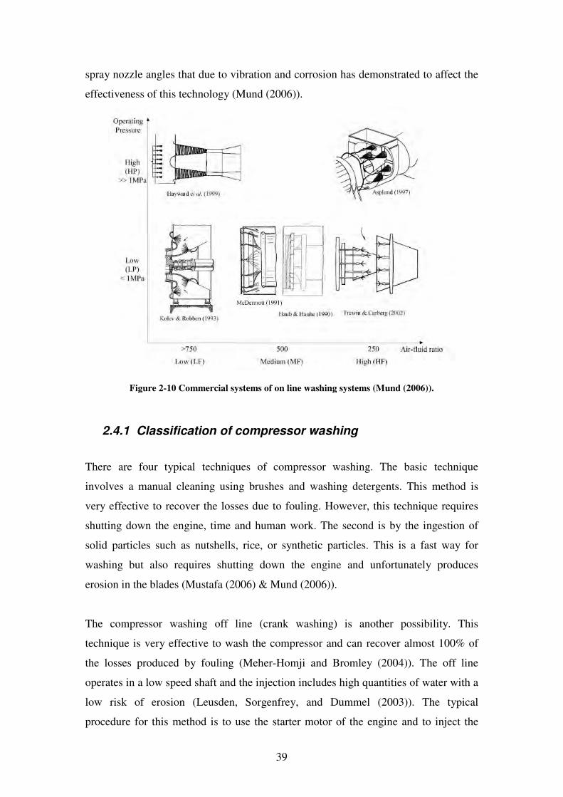
39
spray nozzle angles that due to vibration and corrosion has demonstrated to affect the
effectiveness of this technology (Mund (2006)).
Figure 2-10 Commercial systems of on line washing systems (Mund (2006)).
2.4.1 Classification of compressor washing
There are four typical techniques of compressor washing. The basic technique
involves a manual cleaning using brushes and washing detergents. This method is
very effective to recover the losses due to fouling. However, this technique requires
shutting down the engine, time and human work. The second is by the ingestion of
solid particles such as nutshells, rice, or synthetic particles. This is a fast way for
washing but also requires shutting down the engine and unfortunately produces
erosion in the blades (Mustafa (2006) & Mund (2006)).
The compressor washing off line (crank washing) is another possibility. This
technique is very effective to wash the compressor and can recover almost 100% of
the losses produced by fouling (Meher-Homji and Bromley (2004)). The off line
operates in a low speed shaft and the injection includes high quantities of water with a
low risk of erosion (Leusden, Sorgenfrey, and Dummel (2003)). The typical
procedure for this method is to use the starter motor of the engine and to inject the
40
cleaning detergent into the inlet. In this process the cleaning fluid passes through all
the compressor stages and the wash is drained away (Fielder (2003)).
The disadvantage of washing off line is that only it is possible to operate when the
engine is shutting down (Meher-Homji and Bromley (2004)). In addition, running the
shaft at a low speed reduces the starter motor life of the engine and then increases the
washing costs. This last problem is important in places where the space is limited or
where it is necessary to produce the water as such as ships and offshore rigs (Fielder
(2003)).
The new technique is compressor washing on line (fired washing) that operates at full
load of engine operation. This maintenance extends the intervals between compressor
washings off-line and corrects automatically the fouling losses produced in the
compressor. The system of compressor washing on line is based on the state of the art
and involves the following characteristics: droplet size, speed and angles of injection
(nozzle location) (Raykowski, Hader, Maragno, and Spelt (2001) & Mund and Pilidis
(2004)). Compressor washing off line and on line are different in three principal
characteristics: number and location of nozzles (more nozzles are required in on line),
quantity of fluid (more liquid is required in off line) and washing effectiveness (better
results in off line) (Stalder and Sire (2001)). Kolkman (1993) commented that
compressor washing on line cleans partial the fouled deposits on the compressor
blade. This last result was recognized in previous studies, but it gives a good
alternative to abate the compressor fouling (Stalder and Van Oosten (1994), Mustafa
(2006) & Mund (2006)).
2.4.2 Cleaning fluids
During the eighties the use of demineralised water, water-detergent mixtures and
water-petroleum solvent were used as cleaning fluid (Mund (2006)). The chemical
formula for the cleaning fluid patented by Woodson, Cooper, White, and Fischer
(1989) increased the boiling point of the water. Later on, the use of anti freezer as
additive in the cleaning fluid allowed the compressor washing under low
temperatures. In the nineties, the improvements of the cleaning fluid resulted to be
41
fully combustible and biodegradable (Kaes (1991)). The use of corrosion inhibitors
mixed with the cleaning fluid increased the effectiveness of compressor washing
(Kolkman (1993)). For example, a marine engine study resulted that the use of anti-
fouling inhibitors gave a smooth finished protection on the surface and un-reactive
dirt or salt deposition (Caguiat (2003)).
The environmental law have limited the use of some chemical products and regulated
the disposition of the cleaning fluid. For example, soil pollution that contains mineral
oils adhered to the airfoils can not be thrown into the drainage. The same case applies
to aromatic-hydrocarbons mixed with the compressor washing cleaner that are
considered harmful to peoples health by skin contact or inhalation (Kolkman (1993)).
However, the improvements on the solvent cleaners have been developed for the use
against the organic pollution (hydrocarbon particles) (Leusden, Sorgenfrey, and
Dummel (2003)). Today three types of fluids are commercially available:
demineralised water, solvents-based and aqueous-based cleaning fluids, but in some
places due to environment regulations the use of solvents is limited (Fielder (2003)).
Information about the chemical formula of the cleaning fluid is not available due to
the policy of the companies (Vigueras Zuniga (2003b)). However, the supplier
guarantee that the cleaning fluid is a water-based formulation, non-toxic, non-
flammable, non-corrosive, readily biodegradable, no harmful effects for the engine
and broad spectrum cleaning of fouled compressor blades (Lambart, Gordon, and
Burnett (2003)). The result of different commercial cleaning fluids can be found in
Harris and Calabrese (1994) publication.
The detergent concentration plays an important part in cleaning the compressor
(Thames, Stegmaier, and Ford (1989)). This because the wet time that the fluid is on
the blades depends on the surface tension and viscosity of the cleaning fluid
(Mezheritsky and Sudarev (1990)). It is important that the cleaning fluid properties
remain liquid (no steam) in the early stages of the compressor. Because, the fouling
deposition is highly dominant in the first four stages and it is almost zero in the rear
stages (Tarabrin, Schurovsky, Bodrov, Stalder, and Bodrov (1998), Fielder (2003) &
Syverud, Brekke, and Bakken (2005)). However, the gas turbine operators and
cleaning fluid suppliers have reported that a hard layer was adhered to the airfoils
42
from the rear stages due to high temperatures that bakes the deposits (Mund and
Pilidis (2004)). For that reason, it is important that the cleaning fluid remain in a
liquid state until the last stages. The chemical composition for the cleaning fluid have
resulted to have solid states of the droplets until 400ºC (sixth stage for typical
industrial axial compressors) (Lambart, Gordon, and Burnett (2003), Asplund (1998)
& Stalder and Sire (2001)). The chemical treatment to improve the evaporation point
can be consulted by Jeffs (1992). The conventional washing fluid can operate in
temperatures around of -10ºC but with the use of anti-cooling mixed with the fluid the
temperature could be lower than -15ºC (Leusden, Sorgenfrey, and Dummel (2003)).
2.4.3 Cleaning fluid injection
The cleaning fluid injection is an essential characteristic of compressor washing on
line. The objective of compressor washing is to wet the more possible region from the
blade surfaces (Meher-Homji and Bromley (2004)). Also, a wet region reduces the
possibility of evaporation of the cleaning fluid and increase the effectiveness of the
washing (Scheper, Mayoral, and Hipp E.J. (1978)). However, the water droplets tend
to follow the air stream and not all the blade surface is wet (Tsuchiya (1982)). For that
reason, the number of nozzles and angles of injection are very important in the
installation of compressor washing on line (Meher-Homji and Bromley (2004) &
Mustafa, (2006)).
The speed and size of the droplet from the injection of compressor washing on line
play an important role to clean the blades surfaces. The numerical study by Mustafa
(2006) demonstrated that that the velocity between the washing liquid and the air is
the parameter that regulates the droplets impact on the blade surface. In this study was
demonstrated that the air stream velocity has a low impact in changing the droplet
size. The selection of the injection angle is a difficult task and involves the centrifugal
and coriolisis effects in the droplet trajectories (see Figure 2-11) (Tsuchiya (1982)).
Mustafa (2006) demonstrated that the angle of injection between 0 to 90 degrees
relative to the air stream direction can reduce the size of the droplet.
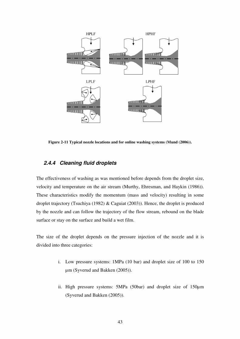
43
Figure 2-11 Typical nozzle locations and for online washing systems (Mund (2006)).
2.4.4 Cleaning fluid droplets
The effectiveness of washing as was mentioned before depends from the droplet size,
velocity and temperature on the air stream (Murthy, Ehresman, and Haykin (1986)).
These characteristics modify the momentum (mass and velocity) resulting in some
droplet trajectory (Tsuchiya (1982) & Caguiat (2003)). Hence, the droplet is produced
by the nozzle and can follow the trajectory of the flow stream, rebound on the blade
surface or stay on the surface and build a wet film.
The size of the droplet depends on the pressure injection of the nozzle and it is
divided into three categories:
i. Low pressure systems: 1MPa (10 bar) and droplet size of 100 to 150
µm (Syverud and Bakken (2005)).
ii. High pressure systems: 5MPa (50bar) and droplet size of 150µm
(Syverud and Bakken (2005)).
44
iii. Nozzle assisted by air: It produces small droplets size at high pressure
systems (Mund (2006)).
The problem of erosion on the airfoils surfaces by water injection has been linked to
impacts from big droplets (Zwebek (2002) & Mustafa (2006)). The different sized
droplets produced from the compressor washing system have been studied in order to
avoid erosion problems*. The results have demonstrated that droplets with a small size
(less 80µm) do not cause erosion (General Electric (2001) & Mustafa (2006)). Meher-
Homji and Bromley (2004) demonstrated that droplets used for the fogging systems
with size between 30 to 40 µm produced non-erosion in the blades. However, the
small droplet size follows the air stream and they do not touch the blade surface
(Mustafa (2006)). Large droplet sizes are more suitable to be in contact with the blade
surfaces and in a short periods they do not represent a problem of erosion (Mustafa
(2006), Lambart, Gordon, and Burnett (2003) & General Electric (2001)).
The phenomenon of rebounding and non-rebounding from the droplet in the
compressor has been studied in different applications. For example, Farrel and Vittal
(1996) demonstrated that small droplets between 18 to 24 µm are non-rebounding in
the inlet of helicopters. However, in the case of industrial application the small
droplet size (less than of 40µm) evaporates due to the ambient temperature (Mustafa
(2006)).
Hayward (1999) suggested an optimal range of droplet size between 80 to 120µm to
clean the first stages and 130 to 170µm to clean the rear stages. The numerical study
from Mustafa (2006) suggested droplets from 50 to 300 µm in a multistage axial
compressor (16 stages). The results are summarized as follows:
• Only large size droplets arrived to the rear stages in the liquid stage
• For engine applications without the presence of salt formation the range of
droplet size suggested is 80 to 160µm (compressor washing on line).
* The erosion mechanism can be consulted the following literature (Tabakoff, Lakshminarasimha, and Pasin (1990), Tabakoff and Balan (1983) & Kurz and Brun (2001)).
45
• For engines with presence of salt formation (offshore or ships) the range of
droplet size suggested is 80 to 800 µm (compressor washing on line)
2.4.5 Engine performance
The engine can recover the losses due to fouling when the compressor washing on
line combines the correct frequency of washing and cleaning fluid (Meher-Homji and
Bromley (2004)). In addition, the engine operation conditions have to be considered
to guarantee an effectiven compressor washing. For example, the ambient temperature
modifies the stage temperature and it affects: the mass flow, the momentum balance
and the evaporation point from the droplet (Mund and Pilidis (2004)). Mustafa (2006)
presented a schematic graphic (see Figure 2-12) to explain the evaporation point of
the droplets according to the compressor stages.
Haub and Hauhe (1990) and Flashberg (1992) agree that compressor washing on line
reduces the total power losses by 3%. Compressor washing on line have demonstrated
to reduce significantly the costs of maintenance (Peltier and Swanekamp (1995),
Leusden, Sorgenfrey, and Dummel (2003) & Stalder and Sire (2001)). Boyce and
Gonzalez (2005) suggested that the theoretical representation of compressor washing
on line recovers the original compressor polytrophic efficiency. According to Orsach,
Kazcprzynski, Roemer, Scharschan, Caguiat, and McGroarty (2002) compressor
washing on line delayed the overall degradation in a rate of 0.2%, but without
washing the degradation increases by 1%. Gulen, Griffin, and Paolucci (2002)
reported a case where compressor washing on line reduced 50% the engine losses
produced by fouling in a period of two months. A successful result of compressor
washing on line involves a study of the system configuration, the level of degradation
and the inlet configuration (Mund (2006)).
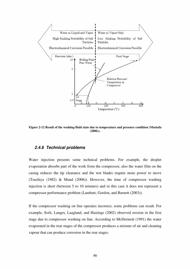
46
Figure 2-12 Result of the washing-fluid state due to temperature and pressure condition (Mustafa
(2006)).
2.4.6 Technical problems
Water injection presents some technical problems. For example, the droplet
evaporation absorbs part of the work from the compressor, also the water film on the
casing reduces the tip clearance and the wet blades require more power to move
(Tsuchiya (1982) & Mund (2006)). However, the time of compressor washing
injection is short (between 5 to 10 minutes) and in this case it does not represent a
compressor performance problem (Lambart, Gordon, and Burnett (2003)).
If the compressor washing on line operates incorrect, some problems can result. For
example, Sorli, Langes, Laagland, and Hastings (2002) observed erosion in the first
stage due to compressor washing on line. According to McDermott (1991) the water
evaporated in the rear stages of the compressor produces a mixture of air and cleaning
vapour that can produce corrosion in the rear stages.
47
There are reports that the results of compressor washing on line were not successful.
Abdelrazik and Cheney (1991) mentioned that compressor washing on line used in a
marine engine did not present any improvement in correcting the engine performance.
According to Gulen, Griffin, and Paolucci (2002) compressor washing on line
produced re-deposition of contaminants from the front to the rear in a multistage
industrial compressor. Yee and Myers (2003) detected that water used for compressor
washing on line in some marine applications contains salts particles that in contact
with the bushings produced corrosion. Thames, Stegmaier, and Ford (1989)
concluded that compressor washing on line is not always the solution to recover the
power from the compressor losses.
2.4.7 Compressor washing frequencies
The compressor washing frequencies has resulted from trials, engine inspections and
operators experience (Fielder (2003)). Information from the literature suggests some
parameters to select the correct compressor washing frequency.
• Mezheritsky and Sudarev (1990) and Diakunchak (1991) suggested the use of
the airflow as a parameter of compressor washing on line (reduction of the
air flow by 2 to 3%).
• Scott (1979) and Syverud, Bakken, Langnes, and Bjornas (2003) suggested
to wash the compressor when the pressure at the inlet of the compressor drops
to 3%.
• Caguiat (2003) suggested the compressor washing on line for marine engine
each 48 to 96 hrs of operation and compressor washing off line each 500 hrs
of operation.
• Boyce and Gonzalez (2005) and Lambart, Gordon, and Burnett (2003)
suggested compressor washing on line for power plants with a frequency of
two times per week.
According to Leusden, Sorgenfrey, and Dummel (2003) the correct frequency of
compressor washing on line can extend the washing off line interval for more than 12
months. Long intervals between compressor washing on line can increase the
48
possibility to remove larger insoluble pieces to the rear stages (Stalder and Van
Oosten (1994) and Stalder and Sire (2001)). However, the best parameter to select the
frequency of compressor washing on line should be based on the fouling level, the
rate deposition and the type of particle adhered, however this information is very
difficult to obtain during the engine operation (Fielder (2003)).
The costs for the cleaning fluid and demineralised water can represent an economical
problem (Mund (2006)). For example, in marine applications the production of clean
water is an extra cost, however in an optimal frequency this system can reduce the
cost of operation by 50% (Fielder (2003)). The study of Syverud, Bakken, Langnes,
and Bjornas (2003) demonstrated that compressor washing on line was economic
rentable and benefit for the operation for an offshore application..
According to Mund (2006) the operation benefits for compressor washing on line are:
• Reduction of engine performance degradation (almost eliminated in some
instances)
• Increments in power production (more kilowatts available to sell)
• Optimal compressor efficiency (operation point stay near of design point)
• Reduction of fuel consumption
• Reduction of the number of shutdowns
• Reduction of time and costs of the maintenance
2.5 Experimental Cascade Rig Tests
The principle of turbomachinery operation is based on diverts the flow from the
blades. In the case of compressors, the flow (air) is compressed and it involves the
change of the physical properties of the air. The use of experimental cascade has been
used for aerodynamic studies in axial compressors. The compressor cascade is defined
as “an infinite row of equidistant similar bodies, these bodies, or blades, are usually
airfoil-shaped” (Gostelow (1984)). A typical configuration of a cascade includes the
arrangement of blades settled inside of an air stream. Depending on the application,
the air stream is produced by external equipment, typically a fan or compressor. The
49
air stream can be produced by positive pressures (blow) or negative pressures
(suction) (Barlow, Rae, and Pope (1999), Gostelow (1984) & Hobson, Hansen,
Schnorenberg, and Grove (2001)).
The experimental cascades are connected to a wind tunnel based on the consideration
that the flow around the body is a relative motion to the body. Hence, the same result
should be obtained if the body is moving or not in a relative uniform velocity flow
(Pankhurts (1952)). It is important to reproduce the similar conditions of viscosity and
density in the experimental cascade according to information from the real situation
(Gostelow (1984) & Pankhurts (1952)).
The wind tunnels are classified into two categories based on the flow velocity (Dixon
(1998)).
i. Low speed wind tunnel is defined by the air stream speeds in the range of 9
to 60 m/s at ISA. In this application, the viscosity forces from the flow are
small and in the practice they are not considered (Hobson, Hansen,
Schnorenberg, and Grove (2001)).
ii. High speed wind tunnel is defined by the air stream speed in the range of
more than 60 m/s at ISA conditions. In this case, the viscosity forces affect the
behaviour of the flow and they have to be considered in the interaction
between surface body and flow (Hobson, Hansen, Schnorenberg, and Grove
(2001)).
The number of blades used in the cascade row is a topic of discussion. Different
criterions have been adopted from previous experiments. The ideal case includes an
infinite number of blades, that in practical situation it is impossible. According to
Dixon (1998) seven blades is the minimum number of blades in the row. However,
the periodicity of the flow from one passage to another passage is the most important
characteristic (Gostelow (1984)). This last characteristic was confirmed by Hobson,
Hansen, Schnorenberg, and Grove (2001) and suggested using the middle passage
from the cascade row blades due to the uniformity and periodicity presented from the
flow. The best approach with real situations is the use of original dimensions for
50
building the cascade. However, the power required for the external equipment to
create the flow condition will be bigger than the original power generated from the
engine ((Dixon (1998) and Pankhurts (1952)). For that reason, small scales from the
blades are used in cascade blade test rigs.
The effect of the floor and ceiling can affect the blade region close to these surfaces.
This problem has been identified due to the boundary layer separation and the three
dimensional effects produced on these surfaces. According with the literature, some
authors have suggested different empirical philosophies to solve this problem. For
example, Gostelow (1984) suggested setting the row blades at one chord distance
from the inlet of the cascade to guarantee that the variation from the pitchwise angle
will be small. Dixon (1998) suggested using blades with a height of aspect ratio* of
three to avoid the effect of the boundary layer separation from the top and bottom
walls.
According to Pankhurts (1952) the benefits of working with wind tunnels give an
opportunity to validate theoretical models. The use of test rigs is safe and relatively
cheap. The results obtained from the experimental cascade represents invaluable
information that due to the complexity are not possible to obtain by theoretical ways
(Gostelow (1984)).
2.5.1 Flow Visualisation
There are many methods to study the flow behaviour in the wind tunnel. One of them
is the technique of visualization in order to describe the flow trajectory. The particle
path technique is commonly used for this application and it consists to describe the air
streamline by the instantaneous position of the particle. This method includes small
particles (liquid drops or solid materials) with fluorescent properties that are delivered
into the air stream. The flow is illuminated and the particles are visible showing the
path of the air stream (Pankhurts (1952)).
* Value obtained from the blade height and chord distance division.
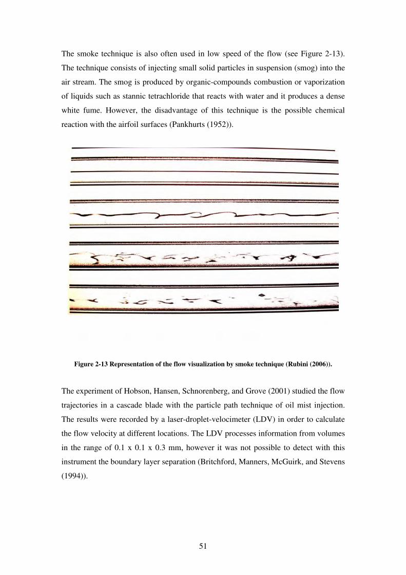
51
The smoke technique is also often used in low speed of the flow (see Figure 2-13).
The technique consists of injecting small solid particles in suspension (smog) into the
air stream. The smog is produced by organic-compounds combustion or vaporization
of liquids such as stannic tetrachloride that reacts with water and it produces a dense
white fume. However, the disadvantage of this technique is the possible chemical
reaction with the airfoil surfaces (Pankhurts (1952)).
Figure 2-13 Representation of the flow visualization by smoke technique (Rubini (2006)).
The experiment of Hobson, Hansen, Schnorenberg, and Grove (2001) studied the flow
trajectories in a cascade blade with the particle path technique of oil mist injection.
The results were recorded by a laser-droplet-velocimeter (LDV) in order to calculate
the flow velocity at different locations. The LDV processes information from volumes
in the range of 0.1 x 0.1 x 0.3 mm, however it was not possible to detect with this
instrument the boundary layer separation (Britchford, Manners, McGuirk, and Stevens
(1994)).
52
2.5.2 Turbulence
Turbulence is a physical phenomenon presented in many engineering flow
applications. The complexity of turbulence involves the solution of the Reynolds
Averaged Navier Stokes (RANS) equations. Turbulence affects the aerodynamic
performance of the airfoils due to movement of the transition point Mayle (1991). The
difficulty to obtain information from the compressor cascade depends on the
turbulence level to know the uniformity of the flow (Hobson, Hansen, Schnorenberg,
and Grove, 2001). The hot wire is an instrument used to calculate the turbulence from
the flow stream in wind tunnels. This device consists of a thin wire resistance made
from platinum connected to voltmeter terminals and located in the air stream. The
estimation of turbulence is made by the change of the electrical current in the
resistance due to the air flow stream.
2.5.3 Boundary layer visualization
The difficulty of visualizing and calculating the boundary layer is due to the micro
scale involved in this phenomenon. In real aerodynamic application it is almost
impossible to measure the velocity profile of the boundary layer (Pankhurts (1952)).
However, the liquid film technique detects on the surface the separation of the
boundary layer or some recirculation. This method consists of the application of a
layer of oil on the surface. The oil evaporation is higher in the turbulence region than
in the laminar region, and then the oil total evaporates after the transition point
(Pankhurts (1952)). The disadvantage of this method is that the oil layer changes the
properties of the surface. However, in many applications the changes are minimum
and these changes can be omitted (Barlow, Rae, and Pope (1999)).
2.5.4 Pressures
The total pressure (stagnation) and static pressure are properties of the flow that can
be measured in wind tunnels to determinate the condition of flow in specific locations
(Pankhurts (1952)). The typical instrument to measure the dynamic pressure is the
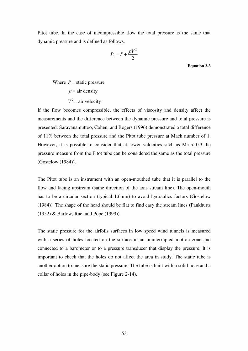
53
Pitot tube. In the case of incompressible flow the total pressure is the same that
dynamic pressure and is defined as follows.
2
2
0
VPP
ρ+=
Equation 2-3
Where P = static pressure
ρ = air density
2V = air velocity
If the flow becomes compressible, the effects of viscosity and density affect the
measurements and the difference between the dynamic pressure and total pressure is
presented. Saravanamuttoo, Cohen, and Rogers (1996) demonstrated a total difference
of 11% between the total pressure and the Pitot tube pressure at Mach number of 1.
However, it is possible to consider that at lower velocities such as Ma < 0.3 the
pressure measure from the Pitot tube can be considered the same as the total pressure
(Gostelow (1984)).
The Pitot tube is an instrument with an open-mouthed tube that it is parallel to the
flow and facing upstream (same direction of the axis stream line). The open-mouth
has to be a circular section (typical 1.6mm) to avoid hydraulics factors (Gostelow
(1984)). The shape of the head should be flat to find easy the stream lines (Pankhurts
(1952) & Barlow, Rae, and Pope (1999)).
The static pressure for the airfoils surfaces in low speed wind tunnels is measured
with a series of holes located on the surface in an uninterrupted motion zone and
connected to a barometer or to a pressure transducer that display the pressure. It is
important to check that the holes do not affect the area in study. The static tube is
another option to measure the static pressure. The tube is built with a solid nose and a
collar of holes in the pipe-body (see Figure 2-14).
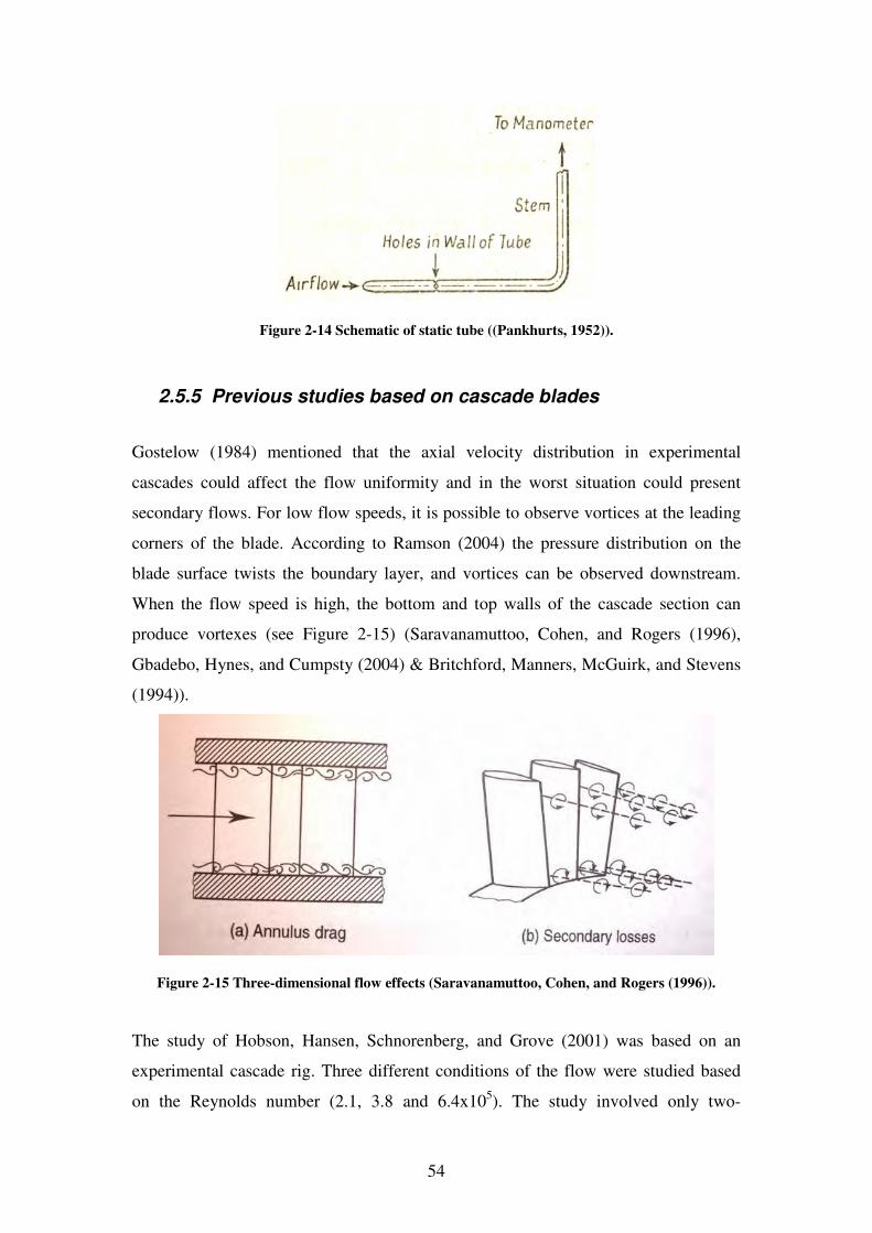
54
Figure 2-14 Schematic of static tube ((Pankhurts, 1952)).
2.5.5 Previous studies based on cascade blades
Gostelow (1984) mentioned that the axial velocity distribution in experimental
cascades could affect the flow uniformity and in the worst situation could present
secondary flows. For low flow speeds, it is possible to observe vortices at the leading
corners of the blade. According to Ramson (2004) the pressure distribution on the
blade surface twists the boundary layer, and vortices can be observed downstream.
When the flow speed is high, the bottom and top walls of the cascade section can
produce vortexes (see Figure 2-15) (Saravanamuttoo, Cohen, and Rogers (1996),
Gbadebo, Hynes, and Cumpsty (2004) & Britchford, Manners, McGuirk, and Stevens
(1994)).
Figure 2-15 Three-dimensional flow effects (Saravanamuttoo, Cohen, and Rogers (1996)).
The study of Hobson, Hansen, Schnorenberg, and Grove (2001) was based on an
experimental cascade rig. Three different conditions of the flow were studied based
on the Reynolds number (2.1, 3.8 and 6.4x10⁵). The study involved only two-
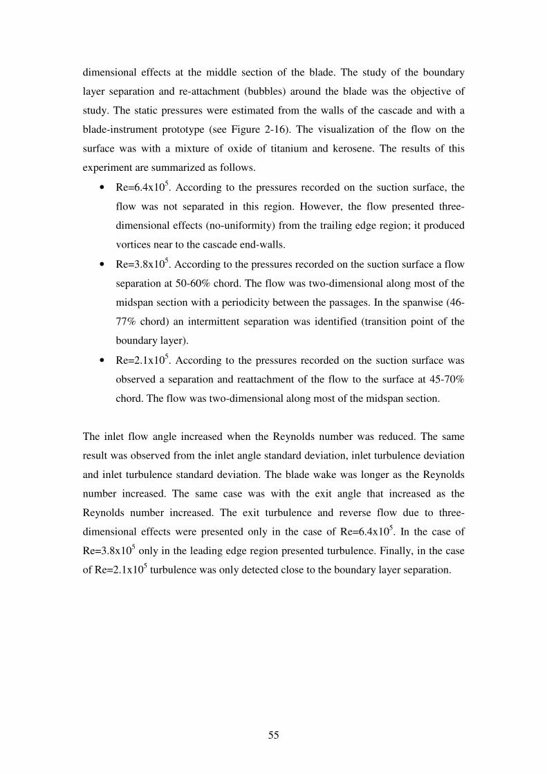
55
dimensional effects at the middle section of the blade. The study of the boundary
layer separation and re-attachment (bubbles) around the blade was the objective of
study. The static pressures were estimated from the walls of the cascade and with a
blade-instrument prototype (see Figure 2-16). The visualization of the flow on the
surface was with a mixture of oxide of titanium and kerosene. The results of this
experiment are summarized as follows.
• Re=6.4x10⁵. According to the pressures recorded on the suction surface, the
flow was not separated in this region. However, the flow presented three-
dimensional effects (no-uniformity) from the trailing edge region; it produced
vortices near to the cascade end-walls.
• Re=3.8x10⁵. According to the pressures recorded on the suction surface a flow
separation at 50-60% chord. The flow was two-dimensional along most of the
midspan section with a periodicity between the passages. In the spanwise (46-
77% chord) an intermittent separation was identified (transition point of the
boundary layer).
• Re=2.1x10⁵. According to the pressures recorded on the suction surface was
observed a separation and reattachment of the flow to the surface at 45-70%
chord. The flow was two-dimensional along most of the midspan section.
The inlet flow angle increased when the Reynolds number was reduced. The same
result was observed from the inlet angle standard deviation, inlet turbulence deviation
and inlet turbulence standard deviation. The blade wake was longer as the Reynolds
number increased. The same case was with the exit angle that increased as the
Reynolds number increased. The exit turbulence and reverse flow due to three-
dimensional effects were presented only in the case of Re=6.4x10⁵. In the case of
Re=3.8x10⁵ only in the leading edge region presented turbulence. Finally, in the case
of Re=2.1x10⁵ turbulence was only detected close to the boundary layer separation.
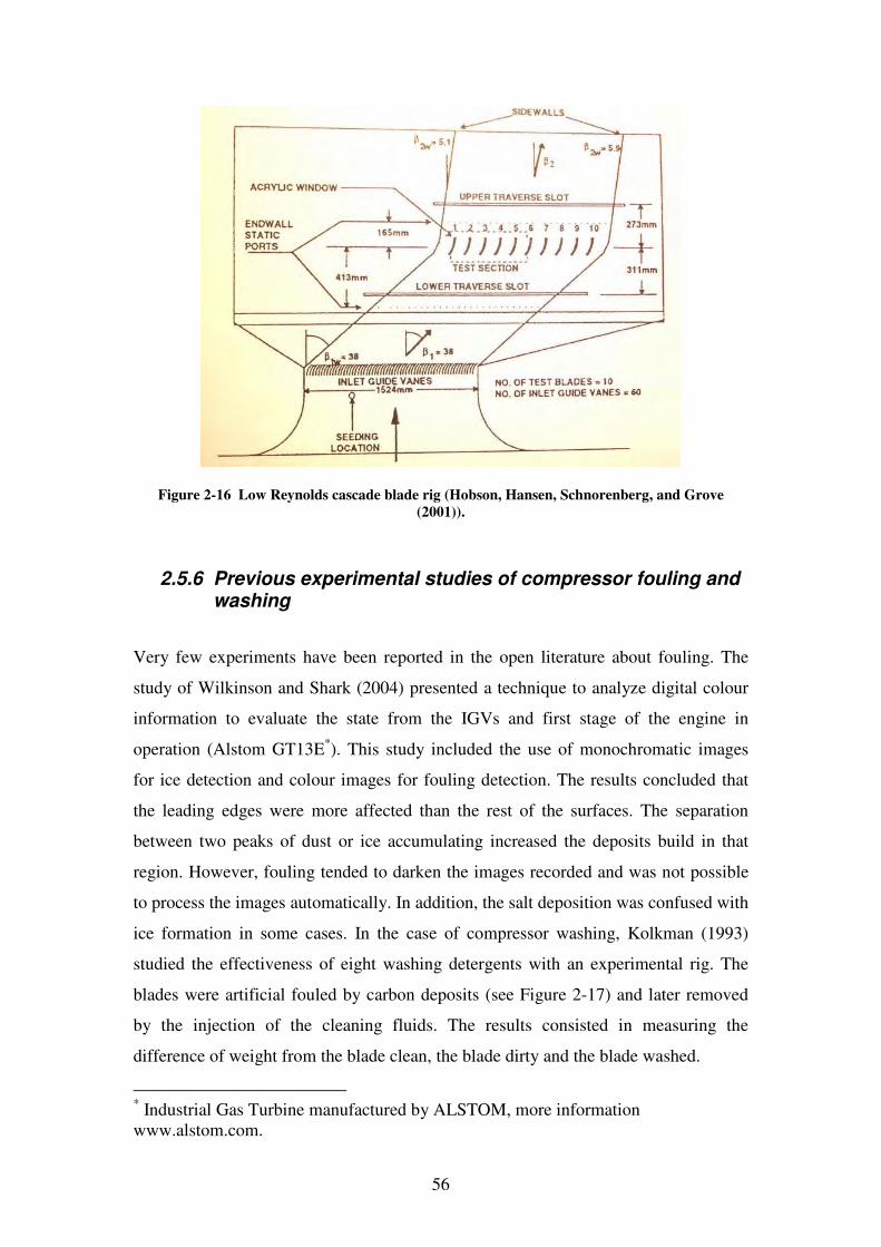
56
Figure 2-16 Low Reynolds cascade blade rig (Hobson, Hansen, Schnorenberg, and Grove
(2001)).
2.5.6 Previous experimental studies of compressor fouling and washing
Very few experiments have been reported in the open literature about fouling. The
study of Wilkinson and Shark (2004) presented a technique to analyze digital colour
information to evaluate the state from the IGVs and first stage of the engine in
operation (Alstom GT13E*). This study included the use of monochromatic images
for ice detection and colour images for fouling detection. The results concluded that
the leading edges were more affected than the rest of the surfaces. The separation
between two peaks of dust or ice accumulating increased the deposits build in that
region. However, fouling tended to darken the images recorded and was not possible
to process the images automatically. In addition, the salt deposition was confused with
ice formation in some cases. In the case of compressor washing, Kolkman (1993)
studied the effectiveness of eight washing detergents with an experimental rig. The
blades were artificial fouled by carbon deposits (see Figure 2-17) and later removed
by the injection of the cleaning fluids. The results consisted in measuring the
difference of weight from the blade clean, the blade dirty and the blade washed.
* Industrial Gas Turbine manufactured by ALSTOM, more information www.alstom.com.
57
Figure 2-17 Configuration of the NLR compressor rig test. Results from particles removed by
the washing process in the rig test (Kolkman (1993)).
Syverud, Brekke, and Bakken (2005) and Syverud and Bakken (2005) presented an
experimental study of compressor washing on line for marine applications. The
engine was artificially deteriorated by water injection mixed with high concentrations
of salt. The deposition of salt was detected by visual inspection and the thickness of
the layer was measured. Due to the difficulties in measuring the roughness from the
engine, an indirect method of image analysis was used. This consisted in comparing
the surface with a standard profile (in this case a standard sand paper grain). The
results demonstrated that the IGV surface the salt accumulation formed a layer in the
hub of 500µm and in the annulus of 25µm. The first stator rotor blade the layer
resulted on the pressure surface by 25 µm and on the suction surface by 10µm.
A similar experiment was reported by Levine and Angello (2005), however the sand
roughness Ks was used to estimate the hydraulic smoothness condition. The results
demonstrated that when Re is less than 90, it is possible to consider that there are no
effects of the roughness parameter that affects the flow.
In this case: 90Re ≤=µ
ρVxKsx
Equation 2-4

58
The study of a degradation mechanism as fouling implies complex and expensive rig
tests (Mustafa (2006)). In addition, the possibility to study this phenomenon in the
real application is very limited due to space and conditions of operation (Fielder,
2003). For that reason, many studies have been based on theoretical results as
numerical analysis and engine performance simulations. Saravanamuttoo and
Lakshminarasimha (1985), Lakshminarasimha and Saravanamutto (1986), Haub and
Hauhe (1990), Flashberg (1992), Tabakoff, Lakshminarasimha, and Pasin (1990),
Mustafa (2006), Mund (2006), etc, agree with the necessity to validate the results with
experimental tests.
59
3 TEST RIG
3.1 Introduction
The information presented in the previous chapter showed that compressor fouling
and washing on line are topics that have not been investigated. Much of the current
information available on this topic was based on theoretical results. Therefore the use
of assumptions and arbitrary factors were inevitable. This has produced uncertainties
from the real effect that fouling represents in the engine operation. The complexity of
isolating the problem inside the engine has limited the studies about engine
degradation mechanisms. For that reason, it is necessary to demonstrate and validate
the theoretical results of previous investigations with experimental studies.
The author and sponsors of this research have decided to make an effort to describe
with a preliminary model the fouling phenomenon in the compressor blades. This
work has used for first time an experimental cascade blade (test rig) to study the
problem of fouling. The description of the test rig design includes the aerodynamic
conditions of the flow, the selection and description of the instrumentation and the
manufacturing process. The aerodynamic conditions of the flow are represented in a
scaled section (cascade) of the first compressor stage. With the information recorded
from the experiment, the phenomenon of compressor fouling will be studied.
3.2 Experimental cascade blade
The test rig design was based on previous experimental studies reported in the
literature. Many of these studies concentrated on salt deposition on blades. In
addition, they were limited to studying the phenomenon outside of the engine due to
the space limitation and operation conditions of the engine. However, in this
experimental investigation the problem of fouling and the process of compressor
washing on line are studied directly from the blade aerodynamics.
60
3.2.1 Particular Objective
The particular objective of this chapter is to design and build the experimental rig.
The study parameters were the inlet conditions of the first compressor stage as
follows.
• Original size of the blade
• Aerodynamic conditions of the first compressor stage at the inlet of the
blade
• Data acquisition of the fouling mechanism in real time
• Control of flow conditions in the test rig
• Analysis of costs for the test rig construction and operation
The design was based on turbomachinery theory, previous experiments and interviews
of specialists in the area. The methodology used to achieve the previous
characteristics of the design was divided into five steps.
1. Specify the flow aerodynamic condition in the test rig.
2. Design a test rig according to the flow condition required.
3. Selection and installation of auxiliary equipment and instrumentation.
4. Specify the process of manufacturing and building of the test rig.
5. Calibrate and validate the operation condition of the test rig with a CFD
model.
3.2.2 Background and source of information
The test rig was designed according to the conditions of operation of an industrial gas
turbine (1.2 MW and mass flow of 6.4kg/s)*. The compressor configuration of this
engine was considered axial-annulus and the original blade size of the first stage was
selected for the design. There is a particular interest from the sponsors of this project
to evaluate the compressor fouling in Combined Cycle Gas Turbines (CCGT) used in
Power Plants. The engine selected to cover this task was a single shaft turbine of
* Similar to this engine is the commercial gas turbine model Saturn-20 of 1.2 MW manufactured by Solar Turbines. This engine is used to drive electrical generators, compressors and pumps in the industry. See Appendix A for further information.
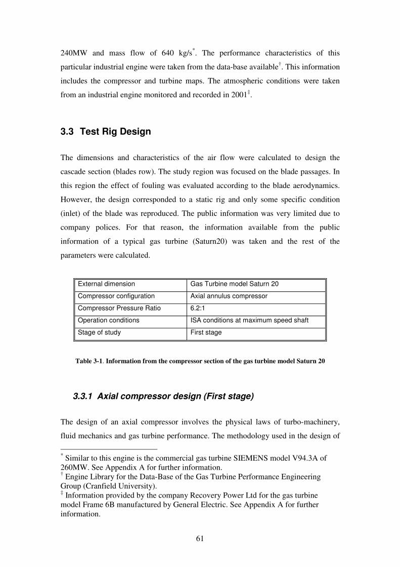
61
240MW and mass flow of 640 kg/s*. The performance characteristics of this
particular industrial engine were taken from the data-base available†. This information
includes the compressor and turbine maps. The atmospheric conditions were taken
from an industrial engine monitored and recorded in 2001‡.
3.3 Test Rig Design
The dimensions and characteristics of the air flow were calculated to design the
cascade section (blades row). The study region was focused on the blade passages. In
this region the effect of fouling was evaluated according to the blade aerodynamics.
However, the design corresponded to a static rig and only some specific condition
(inlet) of the blade was reproduced. The public information was very limited due to
company polices. For that reason, the information available from the public
information of a typical gas turbine (Saturn20) was taken and the rest of the
parameters were calculated.
External dimension Gas Turbine model Saturn 20
Compressor configuration Axial annulus compressor
Compressor Pressure Ratio 6.2:1
Operation conditions ISA conditions at maximum speed shaft
Stage of study First stage
Table 3-1. Information from the compressor section of the gas turbine model Saturn 20
3.3.1 Axial compressor design (First stage)
The design of an axial compressor involves the physical laws of turbo-machinery,
fluid mechanics and gas turbine performance. The methodology used in the design of
* Similar to this engine is the commercial gas turbine SIEMENS model V94.3A of 260MW. See Appendix A for further information. † Engine Library for the Data-Base of the Gas Turbine Performance Engineering Group (Cranfield University). ‡ Information provided by the company Recovery Power Ltd for the gas turbine model Frame 6B manufactured by General Electric. See Appendix A for further information.
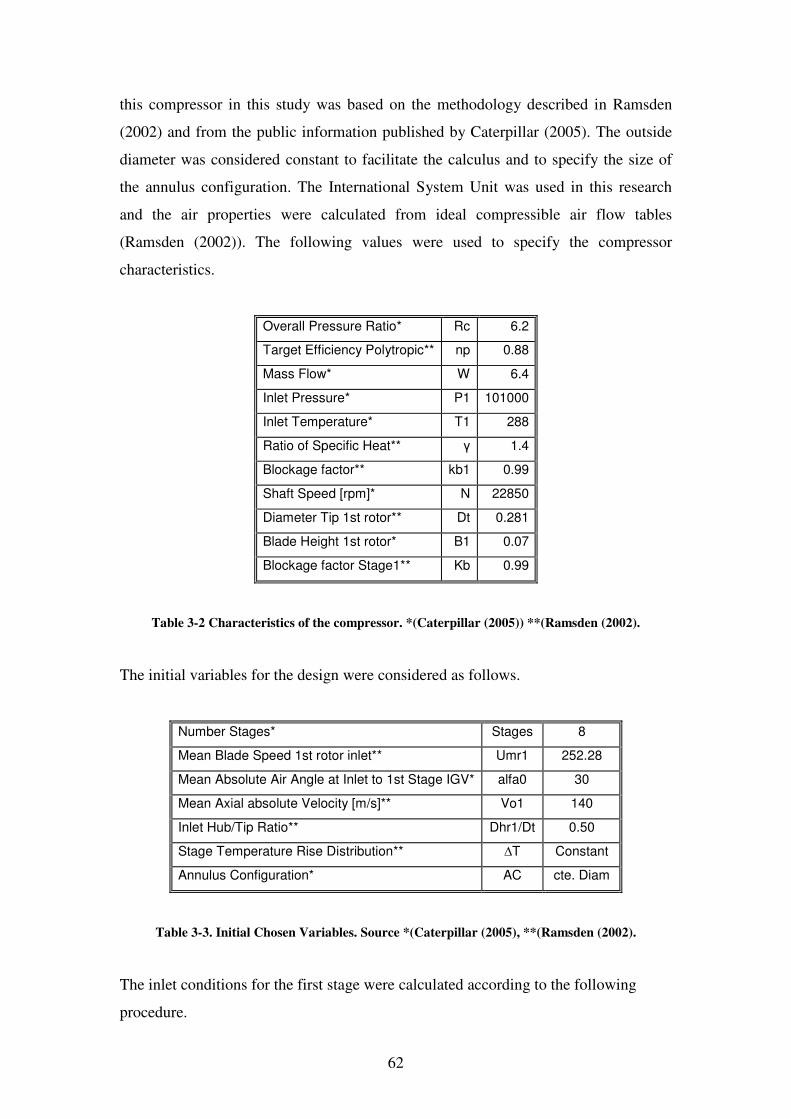
62
this compressor in this study was based on the methodology described in Ramsden
(2002) and from the public information published by Caterpillar (2005). The outside
diameter was considered constant to facilitate the calculus and to specify the size of
the annulus configuration. The International System Unit was used in this research
and the air properties were calculated from ideal compressible air flow tables
(Ramsden (2002)). The following values were used to specify the compressor
characteristics.
Overall Pressure Ratio* Rc 6.2
Target Efficiency Polytropic** np 0.88
Mass Flow* W 6.4
Inlet Pressure* P1 101000
Inlet Temperature* T1 288
Ratio of Specific Heat** γ 1.4
Blockage factor** kb1 0.99
Shaft Speed [rpm]* N 22850
Diameter Tip 1st rotor** Dt 0.281
Blade Height 1st rotor* B1 0.07
Blockage factor Stage1** Kb 0.99
Table 3-2 Characteristics of the compressor. *(Caterpillar (2005)) **(Ramsden (2002).
The initial variables for the design were considered as follows.
Number Stages* Stages 8
Mean Blade Speed 1st rotor inlet** Umr1 252.28
Mean Absolute Air Angle at Inlet to 1st Stage IGV* alfa0 30
Mean Axial absolute Velocity [m/s]** Vo1 140
Inlet Hub/Tip Ratio** Dhr1/Dt 0.50
Stage Temperature Rise Distribution** ∆T Constant
Annulus Configuration* AC cte. Diam
Table 3-3. Initial Chosen Variables. Source *(Caterpillar (2005), **(Ramsden (2002).
The inlet conditions for the first stage were calculated according to the following
procedure.
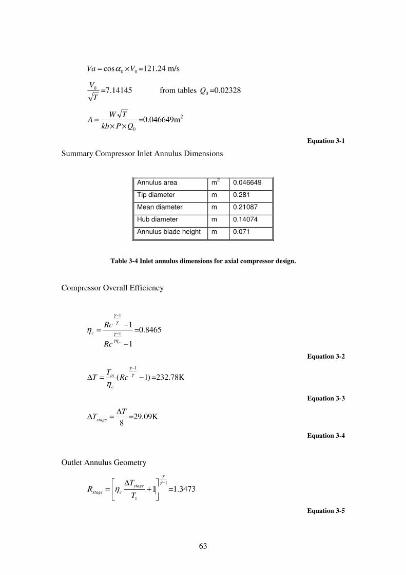
63
00cos VVa ×= α =121.24 m/s
T
V0 =7.14145 from tables 0Q =0.02328
0QPkb
TWA
××= =0.046649m2
Equation 3-1
Summary Compressor Inlet Annulus Dimensions
Annulus area m2
0.046649
Tip diameter m 0.281
Mean diameter m 0.21087
Hub diameter m 0.14074
Annulus blade height m 0.071
Table 3-4 Inlet annulus dimensions for axial compressor design.
Compressor Overall Efficiency
1
11
1
−
−=
−
−
pRc
Rcc
γη
γ
γ
γ
η =0.8465
Equation 3-2
)1(1
−=∆
−
γ
γ
ηRc
TT
c
in =232.78K
Equation 3-3
8
TTstage
∆=∆ =29.09K
Equation 3-4
Outlet Annulus Geometry
1
1
1−
+
∆=
γ
γ
ηT
TR
stage
cstage =1.3473
Equation 3-5
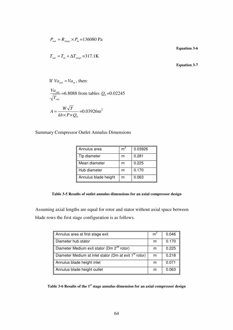
64
instageout PRP ×= =136080 Pa
Equation 3-6
stageinout TTT ∆+= =317.1K
Equation 3-7
If inout VaVa = , then:
out
out
T
Va=6.8088 from tables 0Q =0.02245
0QPkb
TWA
××= =0.03926m2
Summary Compressor Outlet Annulus Dimensions
Annulus area m2
0.03926
Tip diameter m 0.281
Mean diameter m 0.225
Hub diameter m 0.170
Annulus blade height m 0.063
Table 3-5 Results of outlet annulus dimensions for an axial compressor design
Assuming axial lengths are equal for rotor and stator without axial space between
blade rows the first stage configuration is as follows.
Annulus area at first stage exit m2
0.046
Diameter hub stator m 0.170
Diameter Medium exit stator (Dm 2nd
rotor) m 0.225
Diameter Medium at inlet stator (Dm at exit 1st rotor) m 0.218
Annulus blade height inlet m 0.071
Annulus blade height outlet m 0.063
Table 3-6 Results of the 1st stage annulus dimension for an axial compressor design
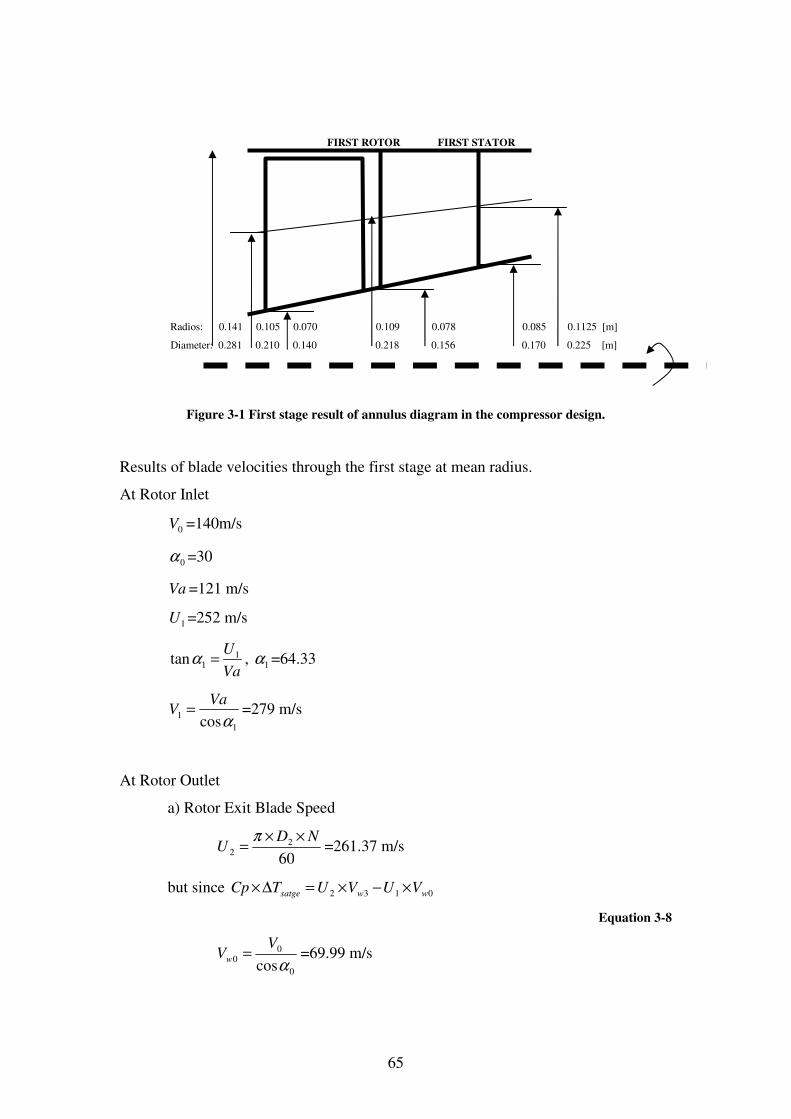
65
FIRST ROTOR FIRST STATOR
Radios: 0.141 0.105 0.070 0.109 0.078 0.085 0.1125 [m]
Diameter: 0.281 0.210 0.140 0.218 0.156 0.170 0.225 [m]
Figure 3-1 First stage result of annulus diagram in the compressor design.
Results of blade velocities through the first stage at mean radius.
At Rotor Inlet
0V =140m/s
0α =30
Va =121 m/s
1U =252 m/s
Va
U11tan =α , 1α =64.33
1
1 cosα
VaV = =279 m/s
At Rotor Outlet
a) Rotor Exit Blade Speed
602
2
NDU
××=
π=261.37 m/s
but since 0132 wwsatge VUVUTCp ×−×=∆×
Equation 3-8
0
00 cosα
VVw = =69.99 m/s
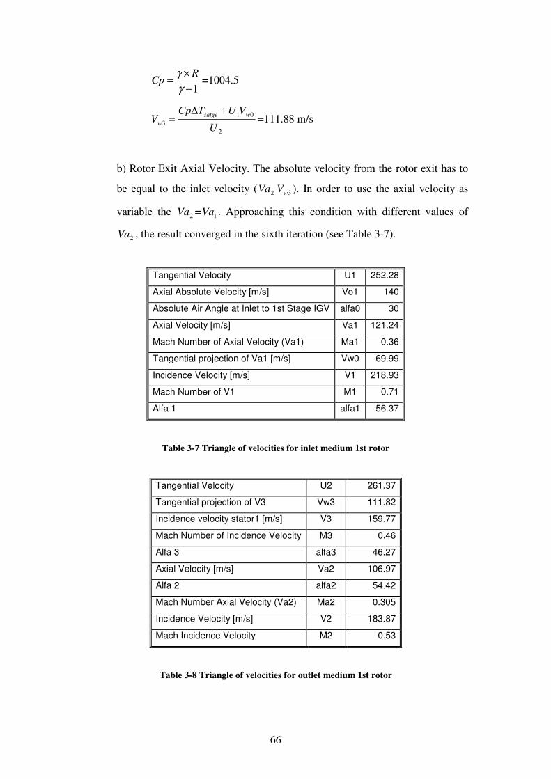
66
1−
×=
γ
γ RCp =1004.5
2
013
U
VUTCpV
wsatge
w
+∆= =111.88 m/s
b) Rotor Exit Axial Velocity. The absolute velocity from the rotor exit has to
be equal to the inlet velocity ( 2Va 3wV ). In order to use the axial velocity as
variable the 2Va = 1Va . Approaching this condition with different values of
2Va , the result converged in the sixth iteration (see Table 3-7).
Tangential Velocity U1 252.28
Axial Absolute Velocity [m/s] Vo1 140
Absolute Air Angle at Inlet to 1st Stage IGV alfa0 30
Axial Velocity [m/s] Va1 121.24
Mach Number of Axial Velocity (Va1) Ma1 0.36
Tangential projection of Va1 [m/s] Vw0 69.99
Incidence Velocity [m/s] V1 218.93
Mach Number of V1 M1 0.71
Alfa 1 alfa1 56.37
Table 3-7 Triangle of velocities for inlet medium 1st rotor
Tangential Velocity U2 261.37
Tangential projection of V3 Vw3 111.82
Incidence velocity stator1 [m/s] V3 159.77
Mach Number of Incidence Velocity M3 0.46
Alfa 3 alfa3 46.27
Axial Velocity [m/s] Va2 106.97
Alfa 2 alfa2 54.42
Mach Number Axial Velocity (Va2) Ma2 0.305
Incidence Velocity [m/s] V2 183.87
Mach Incidence Velocity M2 0.53
Table 3-8 Triangle of velocities for outlet medium 1st rotor
67
Mean Radius Stage Loading Parameters
The following calculations are based on the rotor outlet blade speed
32 wVUTCpH ×=∆=∆
22U
H∆=0.4278
Stage coefficient 2
2
U
Va=0.4092
Then De Haller Number for the rotor results
1
1
2
2
1
2 cos
cos Va
Va
V
VDhr
α
α×== =0.68
Equation 3-9
and De Haller Number for the stator results
2
3
4
1
3
4 cos
cos Va
Va
V
VDhs
α
α×== =0.78
Equation 3-10
The De Haller Number is a common parameter used to predict the limits of the
compressor according to the results of the geometry configuration. This method
consists of estimating the excessive losses based on the compression specification
results from the De Haller Number with a value lower than 0.72.
≥= 12 /VVDh 0.72
Equation 3-11
In the rotor blade the De Haller Number was lower than 0.72. This indicated that
some arbitrary parameters as the angle 0α , shaft speed or dimensions were wrong.
However, these modifications did not take place as they would have resulted in a
change of the original engine size. The result of the preliminary design from the first
stage compressor was considered in the building of the test rig. A final compressor
design should include the following procedure.
• Calculations of all the compressor stages following the same procedure of the
first stage.
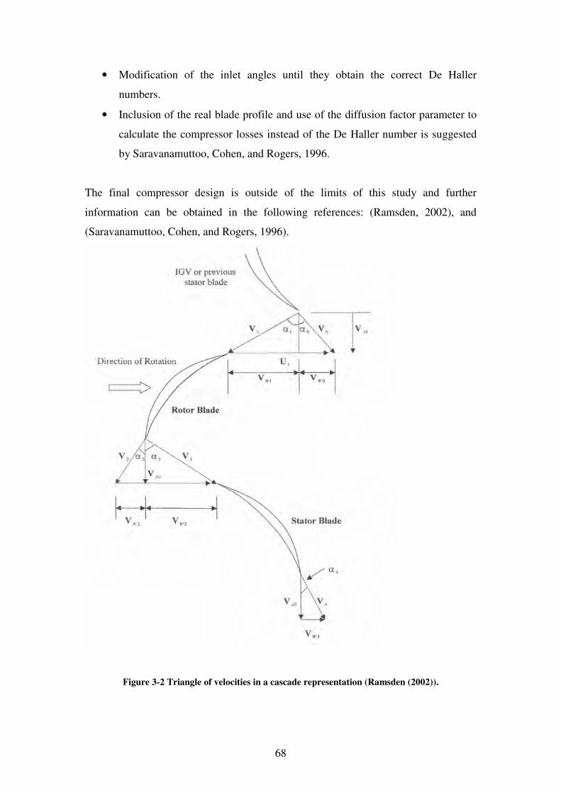
68
• Modification of the inlet angles until they obtain the correct De Haller
numbers.
• Inclusion of the real blade profile and use of the diffusion factor parameter to
calculate the compressor losses instead of the De Haller number is suggested
by Saravanamuttoo, Cohen, and Rogers, 1996.
The final compressor design is outside of the limits of this study and further
information can be obtained in the following references: (Ramsden, 2002), and
(Saravanamuttoo, Cohen, and Rogers, 1996).
Figure 3-2 Triangle of velocities in a cascade representation (Ramsden (2002)).
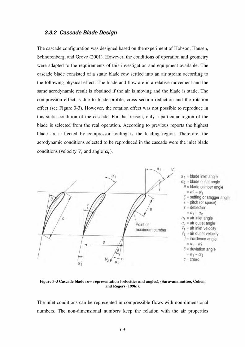
69
3.3.2 Cascade Blade Design
The cascade configuration was designed based on the experiment of Hobson, Hansen,
Schnorenberg, and Grove (2001). However, the conditions of operation and geometry
were adapted to the requirements of this investigation and equipment available. The
cascade blade consisted of a static blade row settled into an air stream according to
the following physical effect: The blade and flow are in a relative movement and the
same aerodynamic result is obtained if the air is moving and the blade is static. The
compression effect is due to blade profile, cross section reduction and the rotation
effect (see Figure 3-3). However, the rotation effect was not possible to reproduce in
this static condition of the cascade. For that reason, only a particular region of the
blade is selected from the real operation. According to previous reports the highest
blade area affected by compressor fouling is the leading region. Therefore, the
aerodynamic conditions selected to be reproduced in the cascade were the inlet blade
conditions (velocity 1V and angle 1α ).
Figure 3-3 Cascade blade row representation (velocities and angles), (Saravanamuttoo, Cohen,
and Rogers (1996)).
The inlet conditions can be represented in compressible flows with non-dimensional
numbers. The non-dimensional numbers keep the relation with the air properties
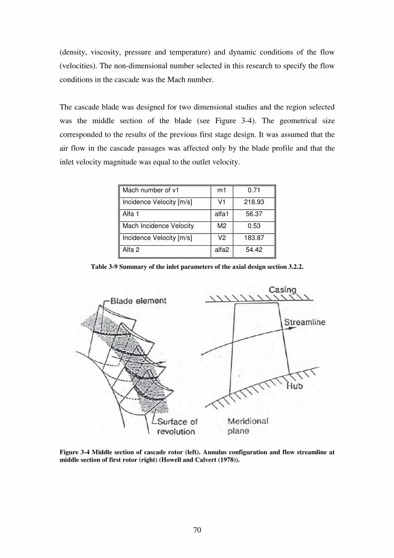
70
(density, viscosity, pressure and temperature) and dynamic conditions of the flow
(velocities). The non-dimensional number selected in this research to specify the flow
conditions in the cascade was the Mach number.
The cascade blade was designed for two dimensional studies and the region selected
was the middle section of the blade (see Figure 3-4). The geometrical size
corresponded to the results of the previous first stage design. It was assumed that the
air flow in the cascade passages was affected only by the blade profile and that the
inlet velocity magnitude was equal to the outlet velocity.
Mach number of v1 m1 0.71
Incidence Velocity [m/s] V1 218.93
Alfa 1 alfa1 56.37
Mach Incidence Velocity M2 0.53
Incidence Velocity [m/s] V2 183.87
Alfa 2 alfa2 54.42
Table 3-9 Summary of the inlet parameters of the axial design section 3.2.2.
Figure 3-4 Middle section of cascade rotor (left). Annulus configuration and flow streamline at
middle section of first rotor (right) (Howell and Calvert (1978)).
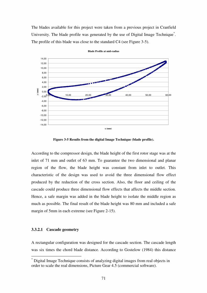
71
The blades available for this project were taken from a previous project in Cranfield
University. The blade profile was generated by the use of Digital Image Technique*.
The profile of this blade was close to the standard C4 (see Figure 3-5).
Blade Profile at mid-radius
-14,00
-12,00
-10,00
-8,00
-6,00
-4,00
-2,00
0,00
2,00
4,00
6,00
8,00
10,00
12,00
14,00
0,00 10,00 20,00 30,00 40,00 50,00 60,00
x (mm)
y (
mm
)
Figure 3-5 Results from the digital Image Technique (blade profile).
According to the compressor design, the blade height of the first rotor stage was at the
inlet of 71 mm and outlet of 63 mm. To guarantee the two dimensional and planar
region of the flow, the blade height was constant from inlet to outlet. This
characteristic of the design was used to avoid the three dimensional flow effect
produced by the reduction of the cross section. Also, the floor and ceiling of the
cascade could produce three dimensional flow effects that affects the middle section.
Hence, a safe margin was added in the blade height to isolate the middle region as
much as possible. The final result of the blade height was 80 mm and included a safe
margin of 5mm in each extreme (see Figure 2-15).
3.3.2.1 Cascade geometry
A rectangular configuration was designed for the cascade section. The cascade length
was six times the chord blade distance. According to Gostelow (1984) this distance
* Digital Image Technique consists of analyzing digital images from real objects in order to scale the real dimensions, Picture Gear 4.5 (commercial software).

72
helps to obtain equal velocities at inlet and outlet 21 VV = (Hobson, Hansen,
Schnorenberg, and Grove (2001)). The blade row has to be settled one chord distance
from the inlet of the cascade for a uniform flow in the blade passages. The distance
between each passage was calculated with the dimensions of the middle-section and
resulted in a distance of 40mm.
The inlet velocity of the cascade was the incidence blade velocity ( 1V ). The blades
were settled according to the air inlet angle ( 1α ) and the incidence blade angle ( j )* .
The outlet angles were defined by the blade profile.
Figure 3-6 Middle section plane representation in a real blade row (Gostelow (1984)).
The Cartesian coordinates system was adopted in this research due to the absence of
rotation. The axis configuration was as follows.
+X in the direction of 1V
+Y in the direction of the passages
+Z in the direction of the height
* The blade angle ( j ) and outlet angle were defined according to the blade profile.
X
Y
Z
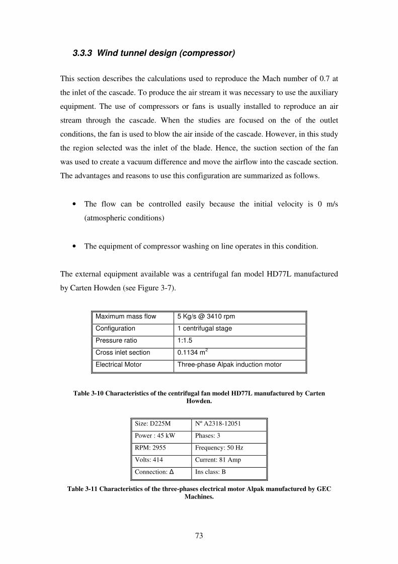
73
3.3.3 Wind tunnel design (compressor)
This section describes the calculations used to reproduce the Mach number of 0.7 at
the inlet of the cascade. To produce the air stream it was necessary to use the auxiliary
equipment. The use of compressors or fans is usually installed to reproduce an air
stream through the cascade. When the studies are focused on the of the outlet
conditions, the fan is used to blow the air inside of the cascade. However, in this study
the region selected was the inlet of the blade. Hence, the suction section of the fan
was used to create a vacuum difference and move the airflow into the cascade section.
The advantages and reasons to use this configuration are summarized as follows.
• The flow can be controlled easily because the initial velocity is 0 m/s
(atmospheric conditions)
• The equipment of compressor washing on line operates in this condition.
The external equipment available was a centrifugal fan model HD77L manufactured
by Carten Howden (see Figure 3-7).
Maximum mass flow 5 Kg/s @ 3410 rpm
Configuration 1 centrifugal stage
Pressure ratio 1:1.5
Cross inlet section 0.1134 m2
Electrical Motor Three-phase Alpak induction motor
Table 3-10 Characteristics of the centrifugal fan model HD77L manufactured by Carten
Howden.
Size: D225M Nº A2318-12051
Power : 45 kW Phases: 3
RPM: 2955 Frequency: 50 Hz
Volts: 414 Current: 81 Amp
Connection: ∆ Ins class: B
Table 3-11 Characteristics of the three-phases electrical motor Alpak manufactured by GEC
Machines.
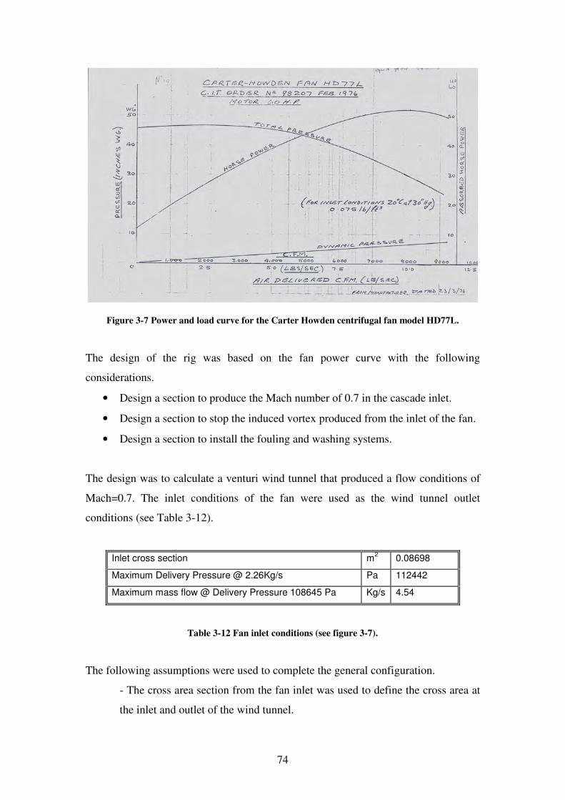
74
Figure 3-7 Power and load curve for the Carter Howden centrifugal fan model HD77L.
The design of the rig was based on the fan power curve with the following
considerations.
• Design a section to produce the Mach number of 0.7 in the cascade inlet.
• Design a section to stop the induced vortex produced from the inlet of the fan.
• Design a section to install the fouling and washing systems.
The design was to calculate a venturi wind tunnel that produced a flow conditions of
Mach=0.7. The inlet conditions of the fan were used as the wind tunnel outlet
conditions (see Table 3-12).
Inlet cross section m2
0.08698
Maximum Delivery Pressure @ 2.26Kg/s Pa 112442
Maximum mass flow @ Delivery Pressure 108645 Pa Kg/s 4.54
Table 3-12 Fan inlet conditions (see figure 3-7).
The following assumptions were used to complete the general configuration.
- The cross area section from the fan inlet was used to define the cross area at
the inlet and outlet of the wind tunnel.
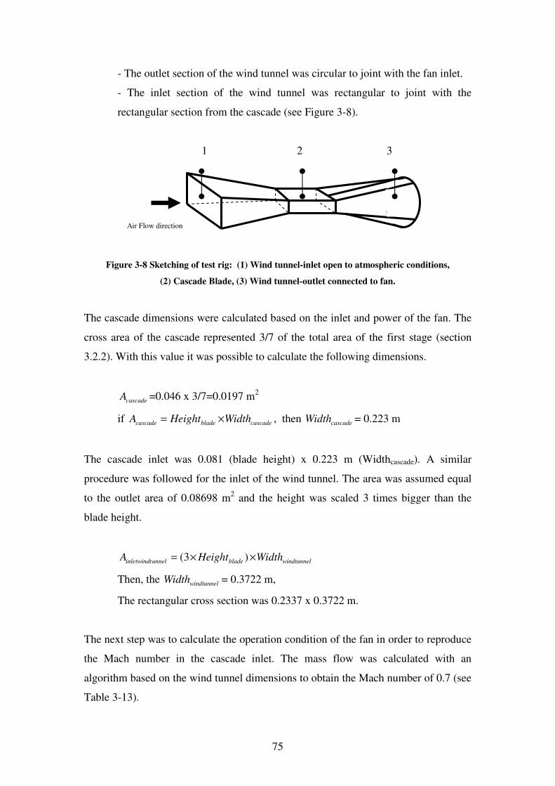
75
- The outlet section of the wind tunnel was circular to joint with the fan inlet.
- The inlet section of the wind tunnel was rectangular to joint with the
rectangular section from the cascade (see Figure 3-8).
1 2 3
Air Flow direction
Figure 3-8 Sketching of test rig: (1) Wind tunnel-inlet open to atmospheric conditions,
(2) Cascade Blade, (3) Wind tunnel-outlet connected to fan.
The cascade dimensions were calculated based on the inlet and power of the fan. The
cross area of the cascade represented 3/7 of the total area of the first stage (section
3.2.2). With this value it was possible to calculate the following dimensions.
cascadeA =0.046 x 3/7=0.0197 m2
if cascadebladecascade WidthHeightA ×= , then cascadeWidth = 0.223 m
The cascade inlet was 0.081 (blade height) x 0.223 m (Widthcascade). A similar
procedure was followed for the inlet of the wind tunnel. The area was assumed equal
to the outlet area of 0.08698 m2 and the height was scaled 3 times bigger than the
blade height.
windtunnelbladeunnelinletwindt WidthHeightA ××= )3(
Then, the windtunnelWidth = 0.3722 m,
The rectangular cross section was 0.2337 x 0.3722 m.
The next step was to calculate the operation condition of the fan in order to reproduce
the Mach number in the cascade inlet. The mass flow was calculated with an
algorithm based on the wind tunnel dimensions to obtain the Mach number of 0.7 (see
Table 3-13).
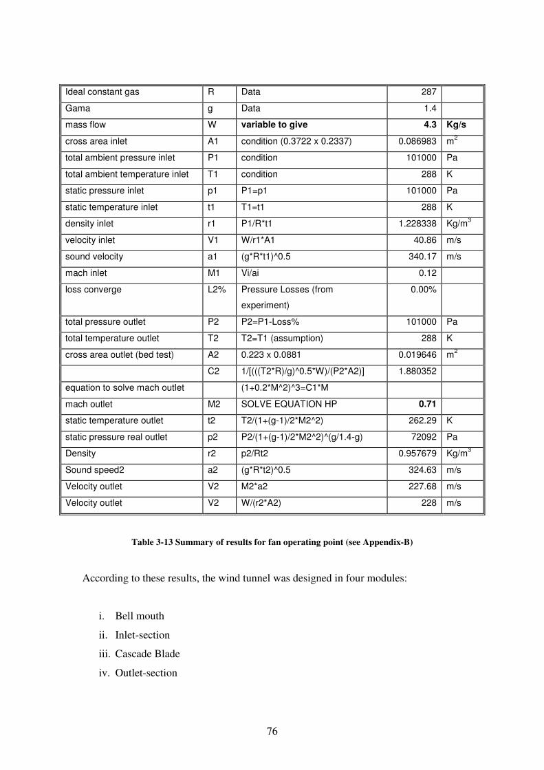
76
Ideal constant gas R Data 287
Gama g Data 1.4
mass flow W variable to give 4.3 Kg/s
cross area inlet A1 condition (0.3722 x 0.2337) 0.086983 m2
total ambient pressure inlet P1 condition 101000 Pa
total ambient temperature inlet T1 condition 288 K
static pressure inlet p1 P1=p1 101000 Pa
static temperature inlet t1 T1=t1 288 K
density inlet r1 P1/R*t1 1.228338 Kg/m3
velocity inlet V1 W/r1*A1 40.86 m/s
sound velocity a1 (g*R*t1)^0.5 340.17 m/s
mach inlet M1 Vi/ai 0.12
loss converge L2% Pressure Losses (from
experiment)
0.00%
total pressure outlet P2 P2=P1-Loss% 101000 Pa
total temperature outlet T2 T2=T1 (assumption) 288 K
cross area outlet (bed test) A2 0.223 x 0.0881 0.019646 m2
C2 1/[(((T2*R)/g)^0.5*W)/(P2*A2)] 1.880352
equation to solve mach outlet (1+0.2*M^2)^3=C1*M
mach outlet M2 SOLVE EQUATION HP 0.71
static temperature outlet t2 T2/(1+(g-1)/2*M2^2) 262.29 K
static pressure real outlet p2 P2/(1+(g-1)/2*M2^2)^(g/1.4-g) 72092 Pa
Density r2 p2/Rt2 0.957679 Kg/m3
Sound speed2 a2 (g*R*t2)^0.5 324.63 m/s
Velocity outlet V2 M2*a2 227.68 m/s
Velocity outlet V2 W/(r2*A2) 228 m/s
Table 3-13 Summary of results for fan operating point (see Appendix-B)
According to these results, the wind tunnel was designed in four modules:
i. Bell mouth
ii. Inlet-section
iii. Cascade Blade
iv. Outlet-section
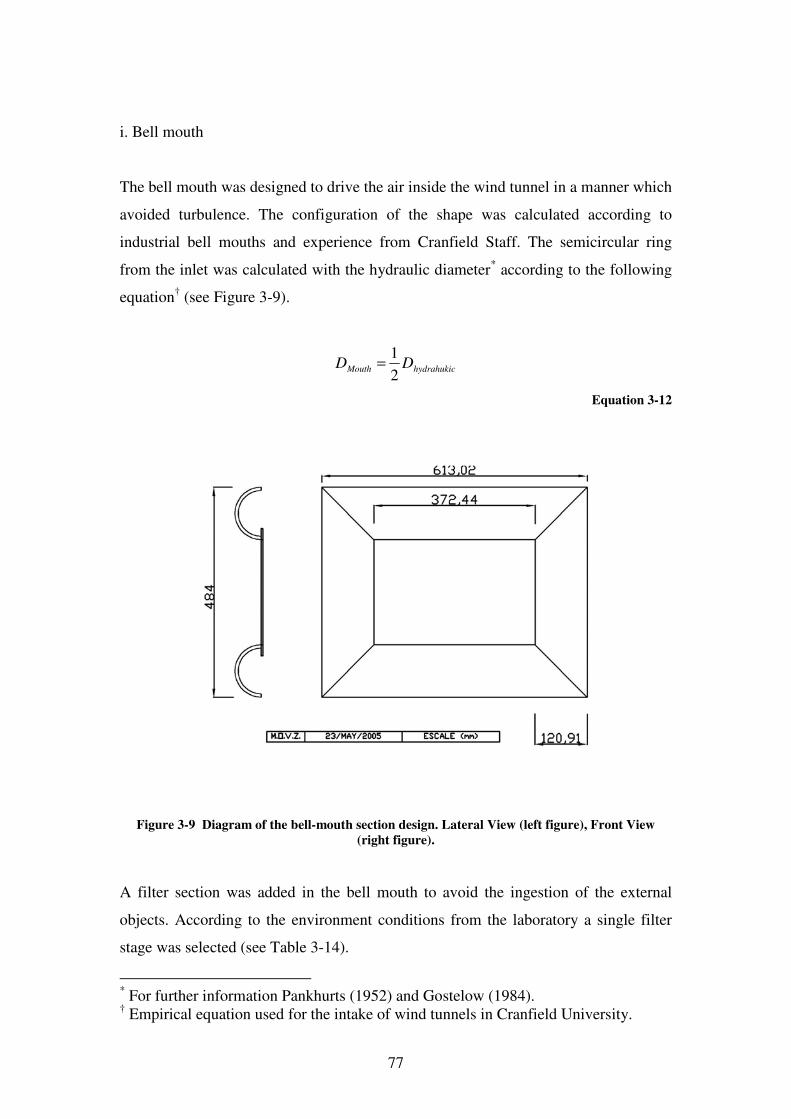
77
i. Bell mouth
The bell mouth was designed to drive the air inside the wind tunnel in a manner which
avoided turbulence. The configuration of the shape was calculated according to
industrial bell mouths and experience from Cranfield Staff. The semicircular ring
from the inlet was calculated with the hydraulic diameter* according to the following
equation† (see Figure 3-9).
hydrahukicMouth DD2
1=
Equation 3-12
Figure 3-9 Diagram of the bell-mouth section design. Lateral View (left figure), Front View
(right figure).
A filter section was added in the bell mouth to avoid the ingestion of the external
objects. According to the environment conditions from the laboratory a single filter
stage was selected (see Table 3-14).
* For further information Pankhurts (1952) and Gostelow (1984). † Empirical equation used for the intake of wind tunnels in Cranfield University.
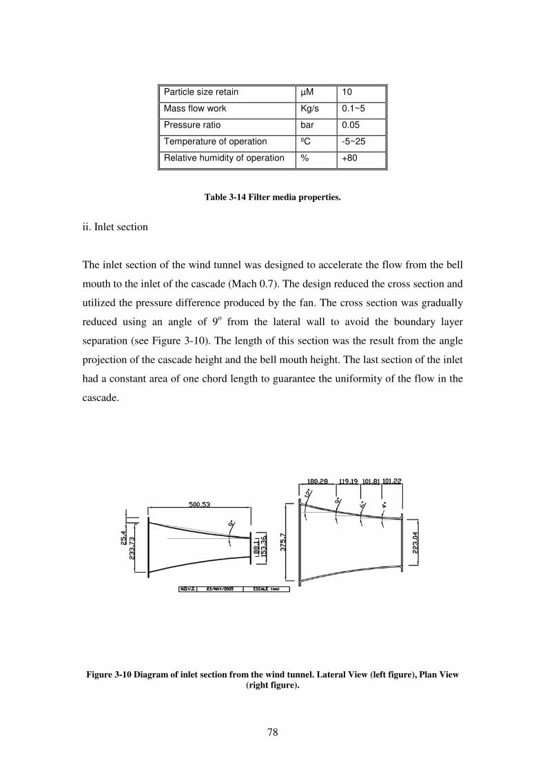
78
Particle size retain µM 10
Mass flow work Kg/s 0.1~5
Pressure ratio bar 0.05
Temperature of operation ºC -5~25
Relative humidity of operation % +80
Table 3-14 Filter media properties.
ii. Inlet section
The inlet section of the wind tunnel was designed to accelerate the flow from the bell
mouth to the inlet of the cascade (Mach 0.7). The design reduced the cross section and
utilized the pressure difference produced by the fan. The cross section was gradually
reduced using an angle of 9o from the lateral wall to avoid the boundary layer
separation (see Figure 3-10). The length of this section was the result from the angle
projection of the cascade height and the bell mouth height. The last section of the inlet
had a constant area of one chord length to guarantee the uniformity of the flow in the
cascade.
Figure 3-10 Diagram of inlet section from the wind tunnel. Lateral View (left figure), Plan View
(right figure).
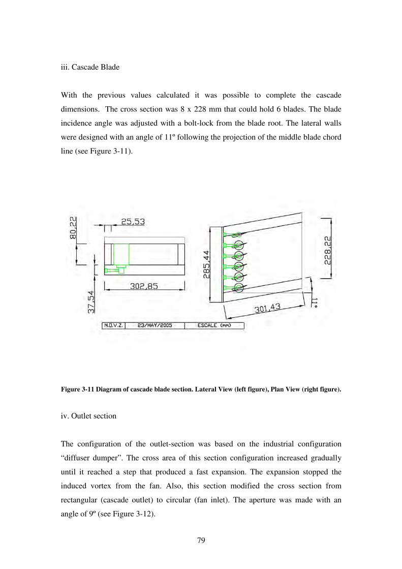
79
iii. Cascade Blade
With the previous values calculated it was possible to complete the cascade
dimensions. The cross section was 8 x 228 mm that could hold 6 blades. The blade
incidence angle was adjusted with a bolt-lock from the blade root. The lateral walls
were designed with an angle of 11º following the projection of the middle blade chord
line (see Figure 3-11).
Figure 3-11 Diagram of cascade blade section. Lateral View (left figure), Plan View (right figure).
iv. Outlet section
The configuration of the outlet-section was based on the industrial configuration
“diffuser dumper”. The cross area of this section configuration increased gradually
until it reached a step that produced a fast expansion. The expansion stopped the
induced vortex from the fan. Also, this section modified the cross section from
rectangular (cascade outlet) to circular (fan inlet). The aperture was made with an
angle of 9º (see Figure 3-12).
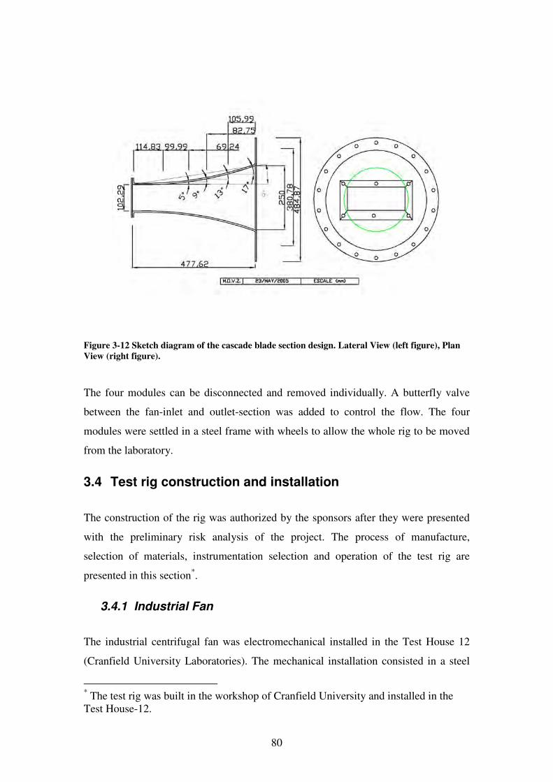
80
Figure 3-12 Sketch diagram of the cascade blade section design. Lateral View (left figure), Plan
View (right figure).
The four modules can be disconnected and removed individually. A butterfly valve
between the fan-inlet and outlet-section was added to control the flow. The four
modules were settled in a steel frame with wheels to allow the whole rig to be moved
from the laboratory.
3.4 Test rig construction and installation
The construction of the rig was authorized by the sponsors after they were presented
with the preliminary risk analysis of the project. The process of manufacture,
selection of materials, instrumentation selection and operation of the test rig are
presented in this section*.
3.4.1 Industrial Fan
The industrial centrifugal fan was electromechanical installed in the Test House 12
(Cranfield University Laboratories). The mechanical installation consisted in a steel
* The test rig was built in the workshop of Cranfield University and installed in the Test House-12.
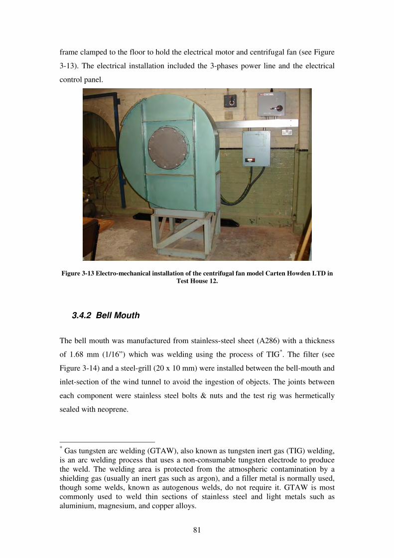
81
frame clamped to the floor to hold the electrical motor and centrifugal fan (see Figure
3-13). The electrical installation included the 3-phases power line and the electrical
control panel.
Figure 3-13 Electro-mechanical installation of the centrifugal fan model Carten Howden LTD in
Test House 12.
3.4.2 Bell Mouth
The bell mouth was manufactured from stainless-steel sheet (A286) with a thickness
of 1.68 mm (1/16”) which was welding using the process of TIG*. The filter (see
Figure 3-14) and a steel-grill (20 x 10 mm) were installed between the bell-mouth and
inlet-section of the wind tunnel to avoid the ingestion of objects. The joints between
each component were stainless steel bolts & nuts and the test rig was hermetically
sealed with neoprene.
* Gas tungsten arc welding (GTAW), also known as tungsten inert gas (TIG) welding, is an arc welding process that uses a non-consumable tungsten electrode to produce the weld. The welding area is protected from the atmospheric contamination by a shielding gas (usually an inert gas such as argon), and a filler metal is normally used, though some welds, known as autogenous welds, do not require it. GTAW is most commonly used to weld thin sections of stainless steel and light metals such as aluminium, magnesium, and copper alloys.
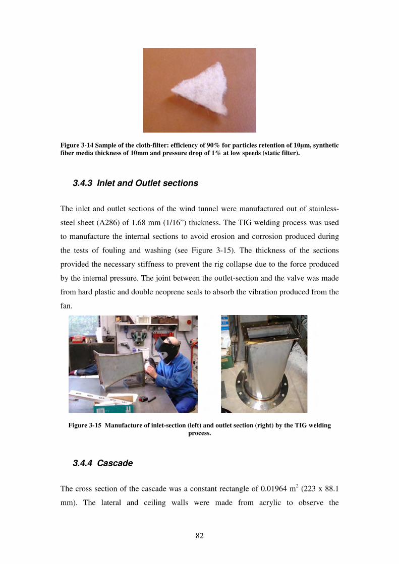
82
Figure 3-14 Sample of the cloth-filter: efficiency of 90% for particles retention of 10µm, synthetic
fiber media thickness of 10mm and pressure drop of 1% at low speeds (static filter).
3.4.3 Inlet and Outlet sections
The inlet and outlet sections of the wind tunnel were manufactured out of stainless-
steel sheet (A286) of 1.68 mm (1/16”) thickness. The TIG welding process was used
to manufacture the internal sections to avoid erosion and corrosion produced during
the tests of fouling and washing (see Figure 3-15). The thickness of the sections
provided the necessary stiffness to prevent the rig collapse due to the force produced
by the internal pressure. The joint between the outlet-section and the valve was made
from hard plastic and double neoprene seals to absorb the vibration produced from the
fan.
Figure 3-15 Manufacture of inlet-section (left) and outlet section (right) by the TIG welding
process.
3.4.4 Cascade
The cross section of the cascade was a constant rectangle of 0.01964 m2 (223 x 88.1
mm). The lateral and ceiling walls were made from acrylic to observe the
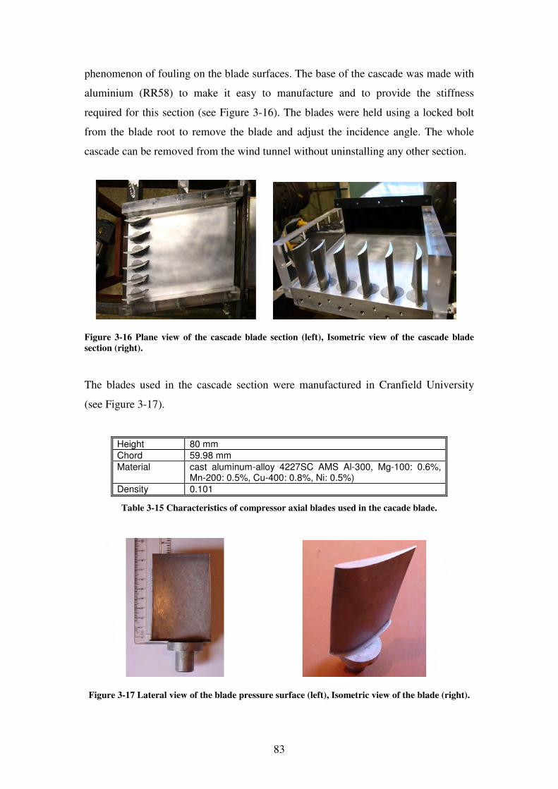
83
phenomenon of fouling on the blade surfaces. The base of the cascade was made with
aluminium (RR58) to make it easy to manufacture and to provide the stiffness
required for this section (see Figure 3-16). The blades were held using a locked bolt
from the blade root to remove the blade and adjust the incidence angle. The whole
cascade can be removed from the wind tunnel without uninstalling any other section.
Figure 3-16 Plane view of the cascade blade section (left), Isometric view of the cascade blade
section (right).
The blades used in the cascade section were manufactured in Cranfield University
(see Figure 3-17).
Height 80 mm
Chord 59.98 mm
Material cast aluminum-alloy 4227SC AMS Al-300, Mg-100: 0.6%, Mn-200: 0.5%, Cu-400: 0.8%, Ni: 0.5%)
Density 0.101
Table 3-15 Characteristics of compressor axial blades used in the cacade blade.
Figure 3-17 Lateral view of the blade pressure surface (left), Isometric view of the blade (right).
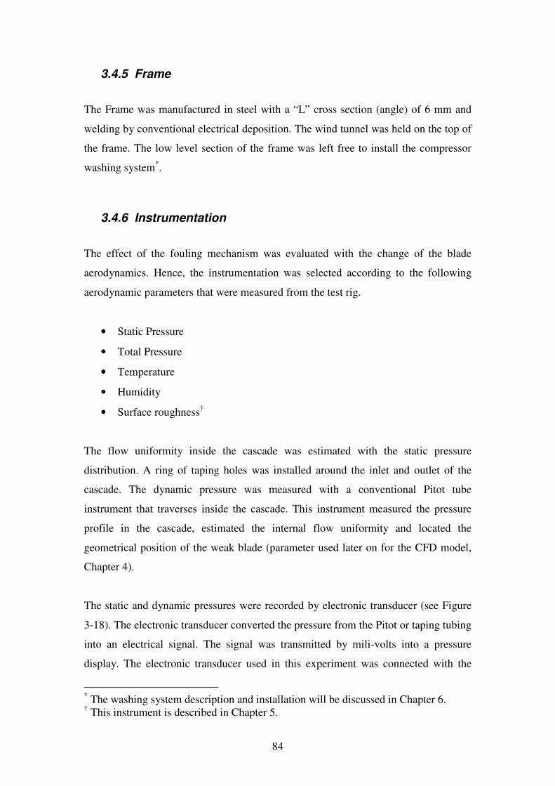
84
3.4.5 Frame
The Frame was manufactured in steel with a “L” cross section (angle) of 6 mm and
welding by conventional electrical deposition. The wind tunnel was held on the top of
the frame. The low level section of the frame was left free to install the compressor
washing system*.
3.4.6 Instrumentation
The effect of the fouling mechanism was evaluated with the change of the blade
aerodynamics. Hence, the instrumentation was selected according to the following
aerodynamic parameters that were measured from the test rig.
• Static Pressure
• Total Pressure
• Temperature
• Humidity
• Surface roughness†
The flow uniformity inside the cascade was estimated with the static pressure
distribution. A ring of taping holes was installed around the inlet and outlet of the
cascade. The dynamic pressure was measured with a conventional Pitot tube
instrument that traverses inside the cascade. This instrument measured the pressure
profile in the cascade, estimated the internal flow uniformity and located the
geometrical position of the weak blade (parameter used later on for the CFD model,
Chapter 4).
The static and dynamic pressures were recorded by electronic transducer (see Figure
3-18). The electronic transducer converted the pressure from the Pitot or taping tubing
into an electrical signal. The signal was transmitted by mili-volts into a pressure
display. The electronic transducer used in this experiment was connected with the
* The washing system description and installation will be discussed in Chapter 6. † This instrument is described in Chapter 5.
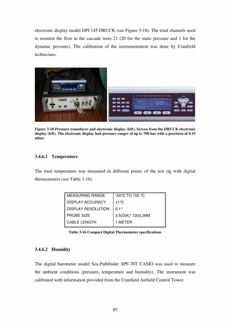
85
electronic display model DPI 145 DRUCK (see Figure 3-18). The total channels used
to monitor the flow in the cascade were 21 (20 for the static pressure and 1 for the
dynamic pressure). The calibration of the instrumentation was done by Cranfield
technicians.
Figure 3-18 Pressure transducer and electronic display (left). Screen from the DRUCK electronic
display (left). The electronic display had pressure ranges of up to 700 bar with a precision of 0.15
mbar.
3.4.6.1 Temperature
The total temperature was measured in different points of the test rig with digital
thermometers (see Table 3-16).
MEASURING RANGE
DISPLAY ACCURACY
DISPLAY RESOLUTION
PROBE SIZE
CABLE LENGTH
-50°C TO 150 °C
±1°C
0.1°
3.5(DIA)* 120(L)MM
1 METER
Table 3-16 Compact Digital Thermometer specifications
3.4.6.2 Humidity
The digital barometer model Sea-Pathfinder SPF-70T CASIO was used to measure
the ambient conditions (pressure, temperature and humidity). The instrument was
calibrated with information provided from the Cranfield Airfield Control Tower.
86
3.4.7 Test Rig Operation Instructions
SAFETY REQUIREMENTS
• Ear defenders and safety glasses
• People and objects must stay away from the wind tunnel inlet and fan outlet
• The wind tunnel should only operate with the protective grill in the wind
tunnel inlet
• To protect the electrical equipment and avoid internal damages due to internal
pressures the valve has to be opened/closed slowly
• Only authorized personnel can operate the equipment and make modifications
OPERATION INSTRUCTIONS
(1) The butterfly valve must be closed before the electrical motor is turned-on
(see Figure 3-20).
(2) Turn-on the energy with the general switch located in control-1 (see Figure 3-
13).
(3) Turned-on the electrical motor with the green button in control-2 and wait
until the 3 phases of the compressor are working at full load which is
indicated by the green light (see Figure 3-13).
(4) Open the valve slowly to achieve operation conditions (se Figure 3-20).
(5) Close the valve slowly to turn off the system (see Figure 3-20).
(6) Turn off the electric motor with the red button in control-2 (see Figure 3-13).
(7) Turn off the energy with the general switch located in control-1 (see Figure 3-
13).
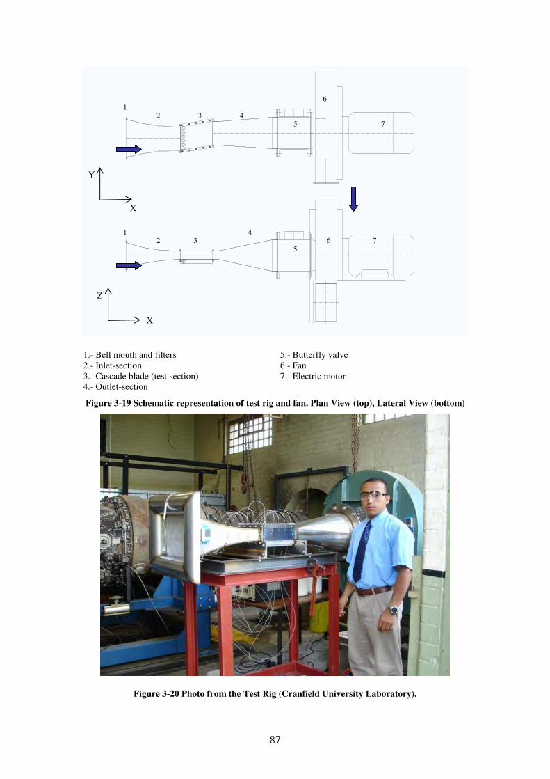
87
1.- Bell mouth and filters 2.- Inlet-section 3.- Cascade blade (test section) 4.- Outlet-section
5.- Butterfly valve 6.- Fan 7.- Electric motor
Figure 3-19 Schematic representation of test rig and fan. Plan View (top), Lateral View (bottom)
Figure 3-20 Photo from the Test Rig (Cranfield University Laboratory).
1 2 3 4
5
6
7
1 2 3
5 6 7
X
Y
Z
X
4
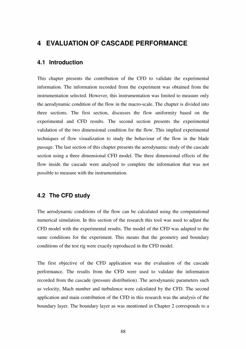
88
4 EVALUATION OF CASCADE PERFORMANCE
4.1 Introduction
This chapter presents the contribution of the CFD to validate the experimental
information. The information recorded from the experiment was obtained from the
instrumentation selected. However, this instrumentation was limited to measure only
the aerodynamic condition of the flow in the macro-scale. The chapter is divided into
three sections. The first section, discusses the flow uniformity based on the
experimental and CFD results. The second section presents the experimental
validation of the two dimensional condition for the flow. This implied experimental
techniques of flow visualization to study the behaviour of the flow in the blade
passage. The last section of this chapter presents the aerodynamic study of the cascade
section using a three dimensional CFD model. The three dimensional effects of the
flow inside the cascade were analysed to complete the information that was not
possible to measure with the instrumentation.
4.2 The CFD study
The aerodynamic conditions of the flow can be calculated using the computational
numerical simulation. In this section of the research this tool was used to adjust the
CFD model with the experimental results. The model of the CFD was adapted to the
same conditions for the experiment. This means that the geometry and boundary
conditions of the test rig were exactly reproduced in the CFD model.
The first objective of the CFD application was the evaluation of the cascade
performance. The results from the CFD were used to validate the information
recorded from the cascade (pressure distribution). The aerodynamic parameters such
as velocity, Mach number and turbulence were calculated by the CFD. The second
application and main contribution of the CFD in this research was the analysis of the
boundary layer. The boundary layer as was mentioned in Chapter 2 corresponds to a
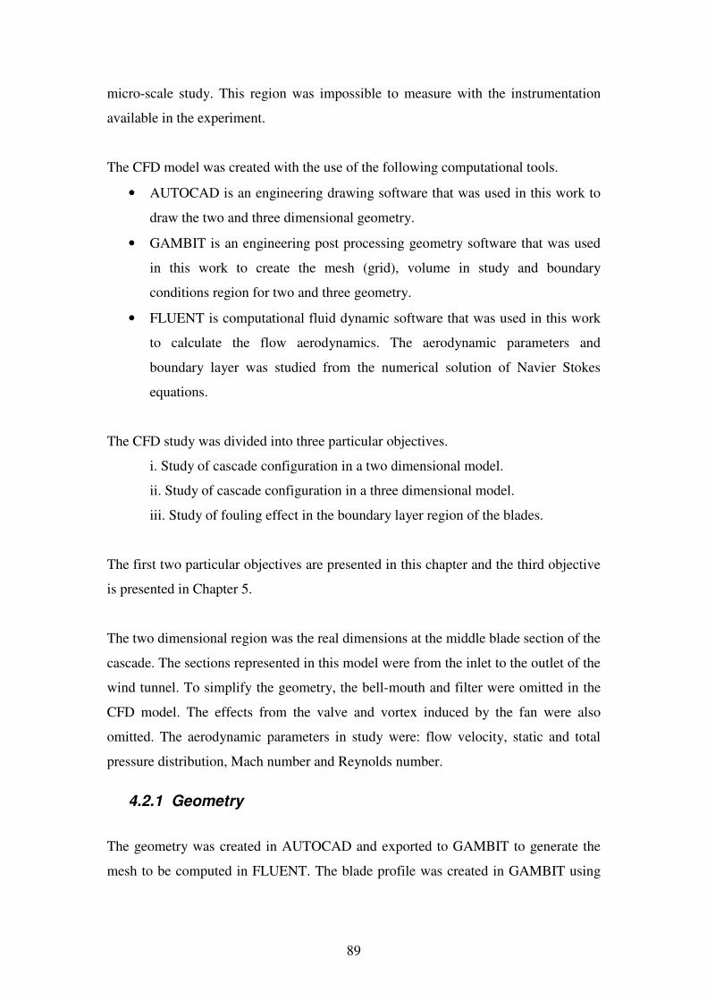
89
micro-scale study. This region was impossible to measure with the instrumentation
available in the experiment.
The CFD model was created with the use of the following computational tools.
• AUTOCAD is an engineering drawing software that was used in this work to
draw the two and three dimensional geometry.
• GAMBIT is an engineering post processing geometry software that was used
in this work to create the mesh (grid), volume in study and boundary
conditions region for two and three geometry.
• FLUENT is computational fluid dynamic software that was used in this work
to calculate the flow aerodynamics. The aerodynamic parameters and
boundary layer was studied from the numerical solution of Navier Stokes
equations.
The CFD study was divided into three particular objectives.
i. Study of cascade configuration in a two dimensional model.
ii. Study of cascade configuration in a three dimensional model.
iii. Study of fouling effect in the boundary layer region of the blades.
The first two particular objectives are presented in this chapter and the third objective
is presented in Chapter 5.
The two dimensional region was the real dimensions at the middle blade section of the
cascade. The sections represented in this model were from the inlet to the outlet of the
wind tunnel. To simplify the geometry, the bell-mouth and filter were omitted in the
CFD model. The effects from the valve and vortex induced by the fan were also
omitted. The aerodynamic parameters in study were: flow velocity, static and total
pressure distribution, Mach number and Reynolds number.
4.2.1 Geometry
The geometry was created in AUTOCAD and exported to GAMBIT to generate the
mesh to be computed in FLUENT. The blade profile was created in GAMBIT using
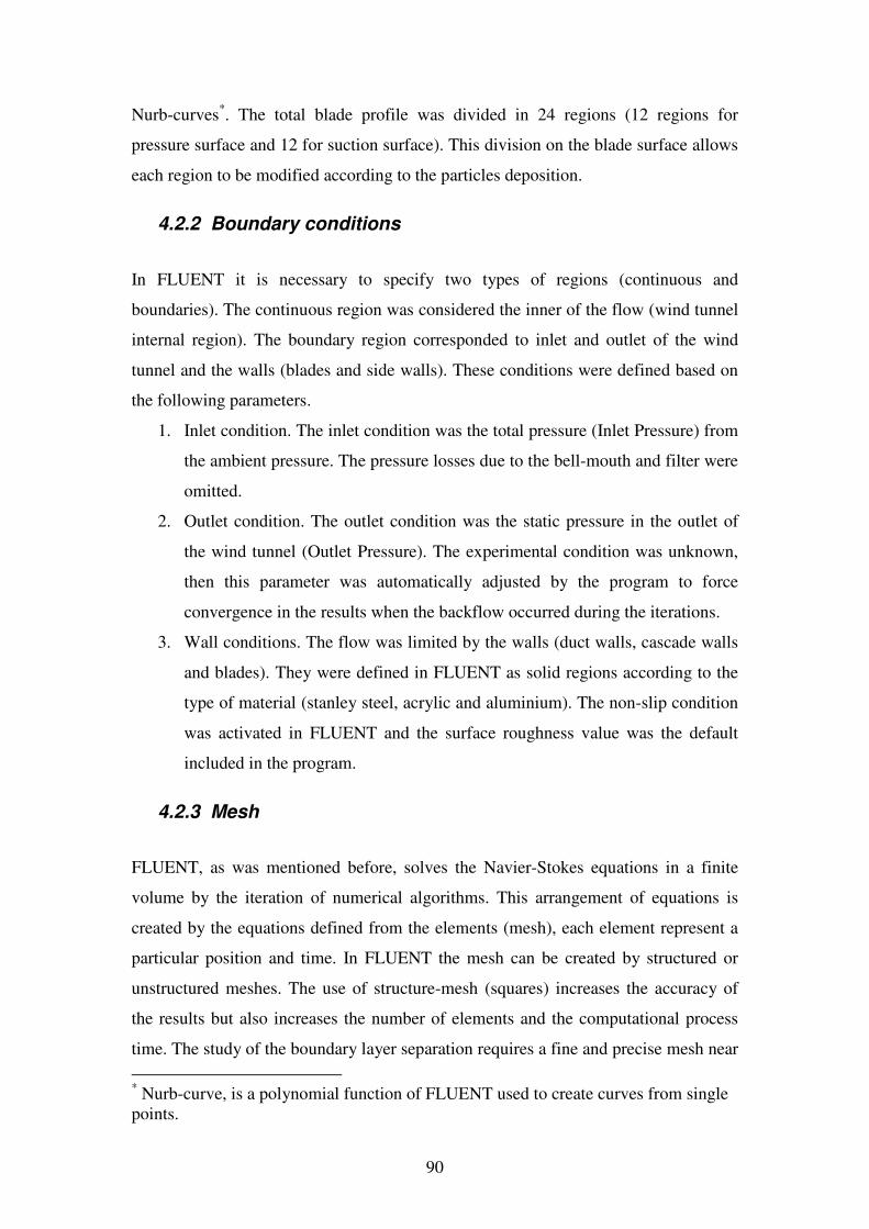
90
Nurb-curves*. The total blade profile was divided in 24 regions (12 regions for
pressure surface and 12 for suction surface). This division on the blade surface allows
each region to be modified according to the particles deposition.
4.2.2 Boundary conditions
In FLUENT it is necessary to specify two types of regions (continuous and
boundaries). The continuous region was considered the inner of the flow (wind tunnel
internal region). The boundary region corresponded to inlet and outlet of the wind
tunnel and the walls (blades and side walls). These conditions were defined based on
the following parameters.
1. Inlet condition. The inlet condition was the total pressure (Inlet Pressure) from
the ambient pressure. The pressure losses due to the bell-mouth and filter were
omitted.
2. Outlet condition. The outlet condition was the static pressure in the outlet of
the wind tunnel (Outlet Pressure). The experimental condition was unknown,
then this parameter was automatically adjusted by the program to force
convergence in the results when the backflow occurred during the iterations.
3. Wall conditions. The flow was limited by the walls (duct walls, cascade walls
and blades). They were defined in FLUENT as solid regions according to the
type of material (stanley steel, acrylic and aluminium). The non-slip condition
was activated in FLUENT and the surface roughness value was the default
included in the program.
4.2.3 Mesh
FLUENT, as was mentioned before, solves the Navier-Stokes equations in a finite
volume by the iteration of numerical algorithms. This arrangement of equations is
created by the equations defined from the elements (mesh), each element represent a
particular position and time. In FLUENT the mesh can be created by structured or
unstructured meshes. The use of structure-mesh (squares) increases the accuracy of
the results but also increases the number of elements and the computational process
time. The study of the boundary layer separation requires a fine and precise mesh near
* Nurb-curve, is a polynomial function of FLUENT used to create curves from single points.
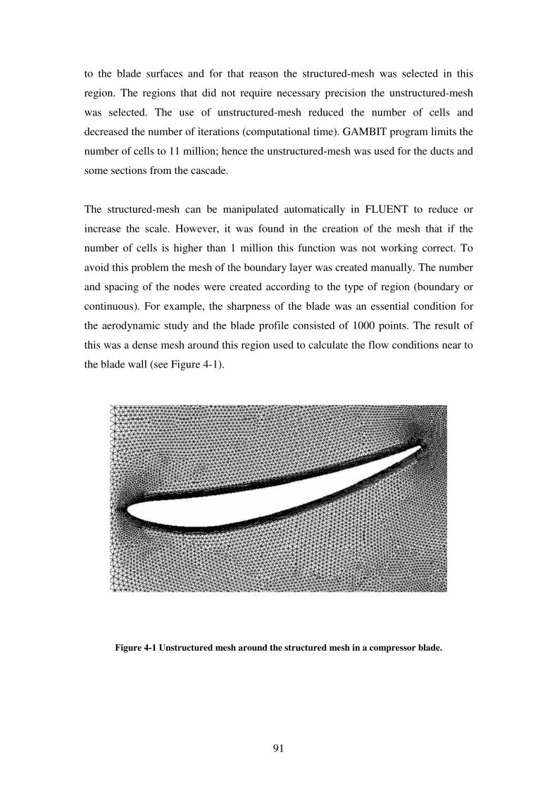
91
to the blade surfaces and for that reason the structured-mesh was selected in this
region. The regions that did not require necessary precision the unstructured-mesh
was selected. The use of unstructured-mesh reduced the number of cells and
decreased the number of iterations (computational time). GAMBIT program limits the
number of cells to 11 million; hence the unstructured-mesh was used for the ducts and
some sections from the cascade.
The structured-mesh can be manipulated automatically in FLUENT to reduce or
increase the scale. However, it was found in the creation of the mesh that if the
number of cells is higher than 1 million this function was not working correct. To
avoid this problem the mesh of the boundary layer was created manually. The number
and spacing of the nodes were created according to the type of region (boundary or
continuous). For example, the sharpness of the blade was an essential condition for
the aerodynamic study and the blade profile consisted of 1000 points. The result of
this was a dense mesh around this region used to calculate the flow conditions near to
the blade wall (see Figure 4-1).
Figure 4-1 Unstructured mesh around the structured mesh in a compressor blade.
92
Figure 4-2 Mesh at leading edge of the blade (left). Mesh at trailing edge of the blade (right).
The flow around the blade near to the surface is laminar and hence the viscous shear
stresses dominate the flow behaviour. But, when the boundary layer starts to separate
the turbulent stresses are presented. The interaction between these two regions has to
be studied carefully in order to determine the transition point. Outside of this region,
the flow can be considered turbulent and it is dominated by the turbulence effect (see
Figure 4-3).
Figure 4-3 Layer treatment near to the wall region (Fluent 2005)
The infinity-velocity U and the wall-shear velocity Ut are scaled by the term u+ as:
tU
Uu =+
Equation 4-1
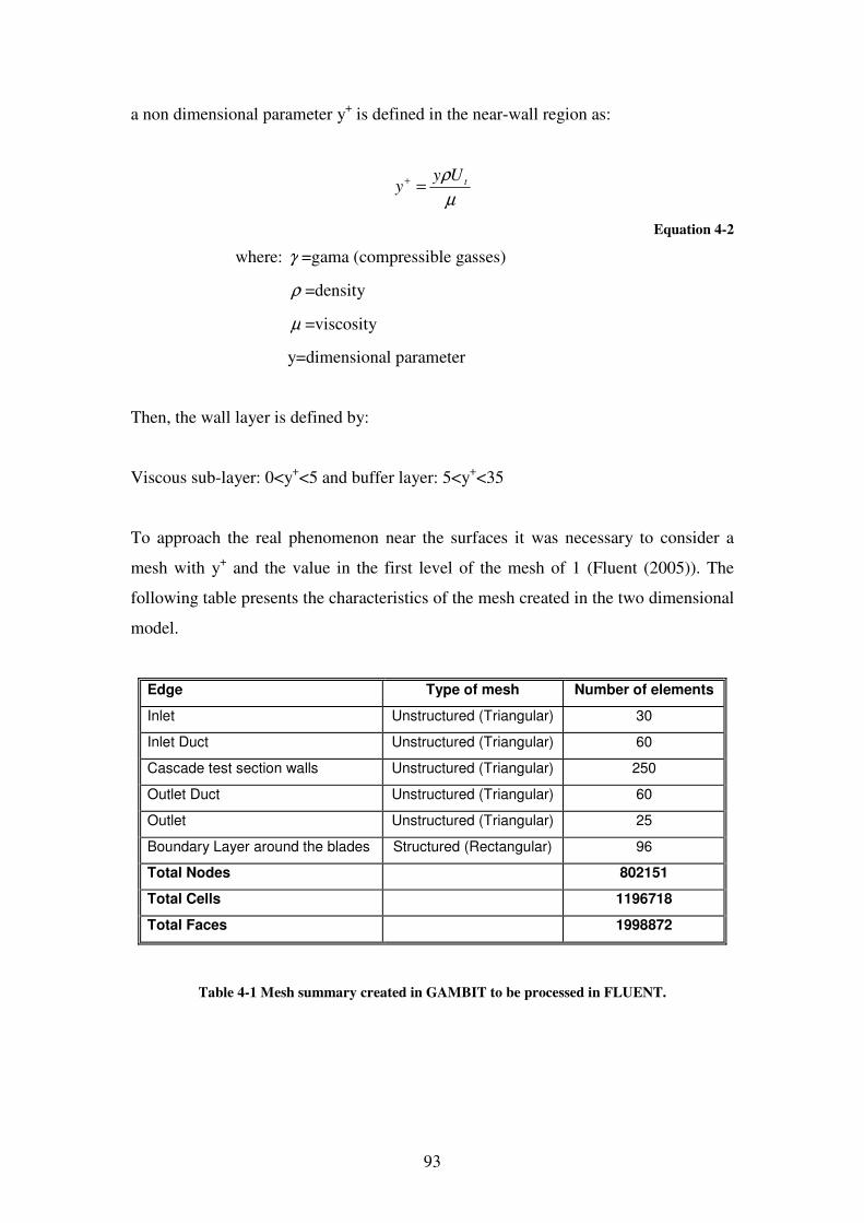
93
a non dimensional parameter y+ is defined in the near-wall region as:
µ
ρ tUyy =+
Equation 4-2
where: γ =gama (compressible gasses)
ρ =density
µ =viscosity
y=dimensional parameter
Then, the wall layer is defined by:
Viscous sub-layer: 0<y+<5 and buffer layer: 5<y+<35
To approach the real phenomenon near the surfaces it was necessary to consider a
mesh with y+ and the value in the first level of the mesh of 1 (Fluent (2005)). The
following table presents the characteristics of the mesh created in the two dimensional
model.
Edge Type of mesh Number of elements
Inlet Unstructured (Triangular) 30
Inlet Duct Unstructured (Triangular) 60
Cascade test section walls Unstructured (Triangular) 250
Outlet Duct Unstructured (Triangular) 60
Outlet Unstructured (Triangular) 25
Boundary Layer around the blades Structured (Rectangular) 96
Total Nodes 802151
Total Cells 1196718
Total Faces 1998872
Table 4-1 Mesh summary created in GAMBIT to be processed in FLUENT.
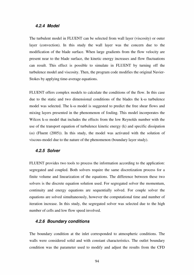
94
4.2.4 Model
The turbulent model in FLUENT can be selected from wall layer (viscosity) or outer
layer (convection). In this study the wall layer was the concern due to the
modification of the blade surface. When large gradients from the flow velocity are
present near to the blade surface, the kinetic energy increases and flow fluctuations
can result. This effect is possible to simulate in FLUENT by turning off the
turbulence model and viscosity. Then, the program code modifies the original Navier-
Stokes by applying time-average equations.
FLUENT offers complex models to calculate the conditions of the flow. In this case
due to the static and two dimensional conditions of the blades the k-ω turbulence
model was selected. The k-ω model is suggested to predict the free shear flows and
mixing layers presented in the phenomenon of fouling. This model incorporates the
Wilcox k-ω model that includes the effects from the low Reynolds number with the
use of the transport equation of turbulence kinetic energy (k) and specific dissipation
(ω) (Fluent (2005)). In this study, the model was activated with the solution of
viscous-model due to the nature of the phenomenon (boundary layer study).
4.2.5 Solver
FLUENT provides two tools to process the information according to the application:
segregated and coupled. Both solvers require the same discretization process for a
finite volume and linearization of the equations. The difference between these two
solvers is the discrete equation solution used. For segregated solver the momentum,
continuity and energy equations are sequentially solved. For couple solver the
equations are solved simultaneously, however the computational time and number of
iteration increase. In this study, the segregated solver was selected due to the high
number of cells and low flow speed involved.
4.2.6 Boundary conditions
The boundary condition at the inlet corresponded to atmospheric conditions. The
walls were considered solid and with constant characteristics. The outlet boundary
condition was the parameter used to modify and adjust the results from the CFD

95
simulation with the experimental results. The following values were used to stabilize
the numerical.
• The inlet velocity at the wind tunnel was different from zero to avoid the
solution diverging in the first iteration.
• The total stagnation temperature at the inlet was 288K (ambient temperature).
• The turbulence was calculated according to the turbulence percentage equation
produced by the grid protection (Osborne (1997)).
( )75
12.1
−
=
d
xTu =2.57%
Equation 4-3
where:
x: is the distance between the grid and blades (0.55 m)
d: is the diameter of the grid bars (0.0028 m)
4.2.7 Parameters of convergence
The parameters of convergence considered in a numerical solution are based on the
experience and judgment of the user. Residual monitors were used as a numerical
parameter of convergence in this study. This included checking the mass flow
continuity according to the limit of difference between inlet and outlet of 1% (Fluent
(2005)). It is also possible to use the drag coefficient as a percentage of error when the
residual monitors do not converge and the result looks stable. The drag coefficient is
useful when the computational time is limited. However in this investigation it was
not necessary to use because the Cranfield network and equipment used in this project
were available to process the information as long as the solution required to converge
from the residual monitors.
The successful procedure to analyze the CFD model is described as follows.
(1) Run the model assuming incompressible flow, constant density and laminar
condition (approximately 10,000 iterations).
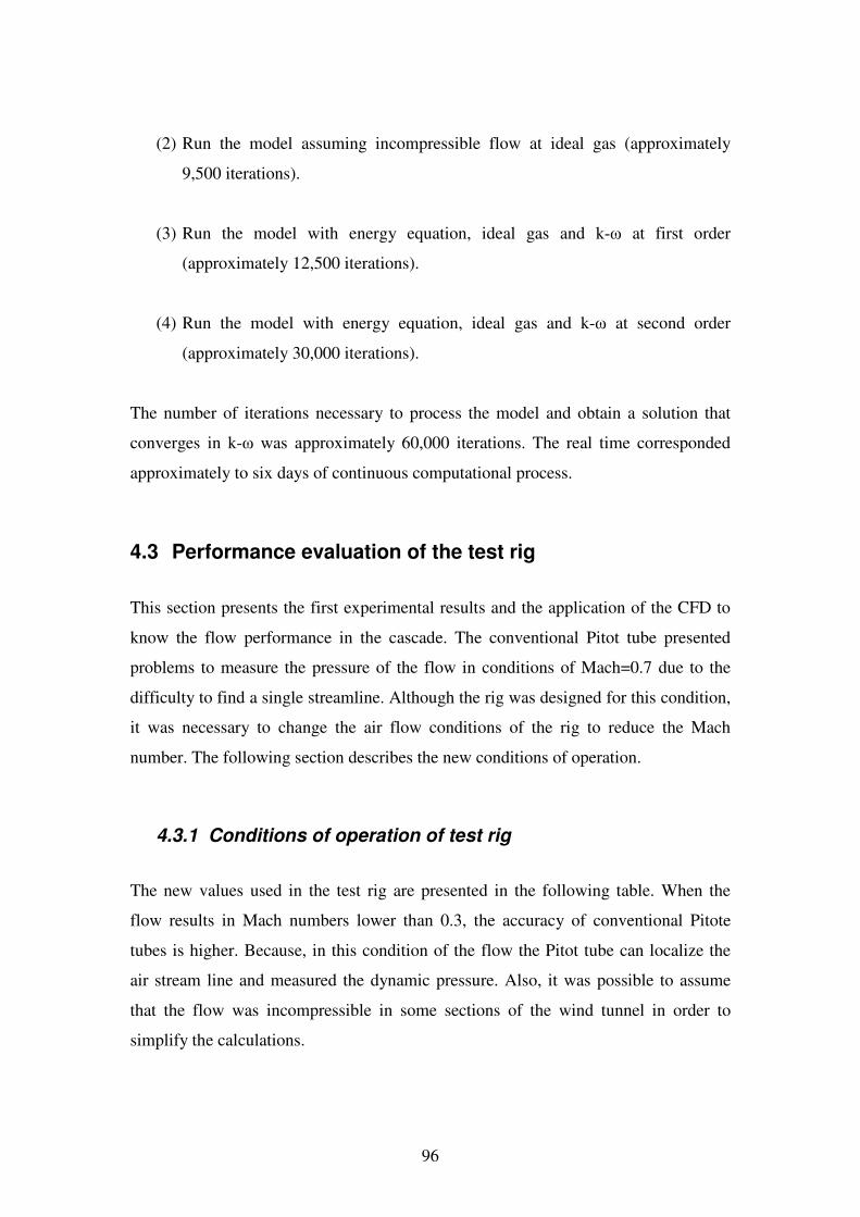
96
(2) Run the model assuming incompressible flow at ideal gas (approximately
9,500 iterations).
(3) Run the model with energy equation, ideal gas and k-ω at first order
(approximately 12,500 iterations).
(4) Run the model with energy equation, ideal gas and k-ω at second order
(approximately 30,000 iterations).
The number of iterations necessary to process the model and obtain a solution that
converges in k-ω was approximately 60,000 iterations. The real time corresponded
approximately to six days of continuous computational process.
4.3 Performance evaluation of the test rig
This section presents the first experimental results and the application of the CFD to
know the flow performance in the cascade. The conventional Pitot tube presented
problems to measure the pressure of the flow in conditions of Mach=0.7 due to the
difficulty to find a single streamline. Although the rig was designed for this condition,
it was necessary to change the air flow conditions of the rig to reduce the Mach
number. The following section describes the new conditions of operation.
4.3.1 Conditions of operation of test rig
The new values used in the test rig are presented in the following table. When the
flow results in Mach numbers lower than 0.3, the accuracy of conventional Pitote
tubes is higher. Because, in this condition of the flow the Pitot tube can localize the
air stream line and measured the dynamic pressure. Also, it was possible to assume
that the flow was incompressible in some sections of the wind tunnel in order to
simplify the calculations.
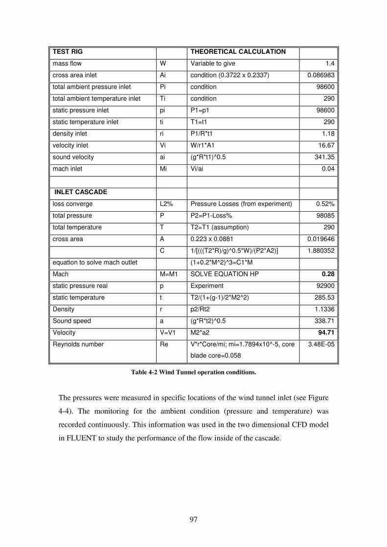
97
TEST RIG THEORETICAL CALCULATION
mass flow W Variable to give 1.4
cross area inlet Ai condition (0.3722 x 0.2337) 0.086983
total ambient pressure inlet Pi condition 98600
total ambient temperature inlet Ti condition 290
static pressure inlet pi P1=p1 98600
static temperature inlet ti T1=t1 290
density inlet ri P1/R*t1 1.18
velocity inlet Vi W/r1*A1 16.67
sound velocity ai (g*R*t1)^0.5 341.35
mach inlet Mi Vi/ai 0.04
INLET CASCADE
loss converge L2% Pressure Losses (from experiment) 0.52%
total pressure P P2=P1-Loss% 98085
total temperature T T2=T1 (assumption) 290
cross area A 0.223 x 0.0881 0.019646
C 1/[(((T2*R)/g)^0.5*W)/(P2*A2)] 1.880352
equation to solve mach outlet (1+0.2*M^2)^3=C1*M
Mach M=M1 SOLVE EQUATION HP 0.28
static pressure real p Experiment 92900
static temperature t T2/(1+(g-1)/2*M2^2) 285.53
Density r p2/Rt2 1.1336
Sound speed a (g*R*t2)^0.5 338.71
Velocity V=V1 M2*a2 94.71
Reynolds number Re V*r*Core/mi; mi=1.7894x10^-5, core
blade core=0.058
3.48E-05
Table 4-2 Wind Tunnel operation conditions.
The pressures were measured in specific locations of the wind tunnel inlet (see Figure
4-4). The monitoring for the ambient condition (pressure and temperature) was
recorded continuously. This information was used in the two dimensional CFD model
in FLUENT to study the performance of the flow inside of the cascade.
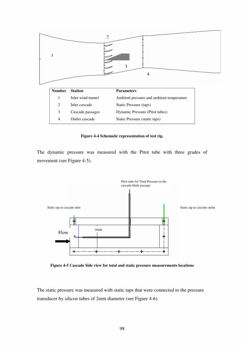
98
Number Station Parameters
1 Inlet wind tunnel Ambient pressure and ambient temperature
2 Inlet cascade Static Pressure (taps)
3 Cascade passages Dynamic Pressure (Pitot tubes)
4 Outlet cascade Static Pressure (static taps)
Figure 4-4 Schematic representation of test rig.
The dynamic pressure was measured with the Pitot tube with three grades of
movement (see Figure 4-5).
Figure 4-5 Cascade Side view for total and static pressure measurements locations
The static pressure was measured with static taps that were connected to the pressure
transducer by silicon tubes of 2mm diameter (see Figure 4-6).
1
2
3
4
Flow
Static tap at cascade inlet Static tap at cascade outlet
Pitot tube for Total Pressure in the cascade blade passage
blade
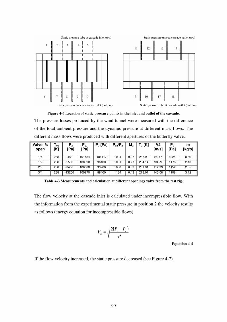
99
Figure 4-6 Location of static pressure points in the inlet and outlet of the cascade.
The pressure losses produced by the wind tunnel were measured with the difference
of the total ambient pressure and the dynamic pressure at different mass flows. The
different mass flows were produced with different apertures of the butterfly valve.
Valve % open
T02 [K]
P2 [Pa]
P02 [Pa]
P2 [Pa] P02/P2 M2 T2 [K] V2 [m/s]
Ρ2 [Pa]
m [kg/s]
1/4 288 -483 101484 101117 1004 0.07 287.90 24.47 1224 0.59
1/2 288 -5500 100990 96100 1051 0.27 284.14 90.29 1178 2.10
2/3 288 -8400 100680 93200 1080 0.33 281.91 112.39 1152 2.55
3/4 288 -13200 100270 88400 1134 0.43 278.01 143.08 1108 3.12
Table 4-3 Measurements and calculation at different openings valve from the test rig.
The flow velocity at the cascade inlet is calculated under incompressible flow. With
the information from the experimental static pressure in position 2 the velocity results
as follows (energy equation for incompressible flows).
( )ρ
212
2 PPV
−=
Equation 4-4
If the flow velocity increased, the static pressure decreased (see Figure 4-7).
Static pressure tube at cascade inlet (top) Static pressure tube at cascade outlet (top)
Static pressure tube at cascade inlet (bottom) Static pressure tube at cascade outlet (bottom)
1 2 3 4 5
6 7 8 9 10
11 12 13 14
15 16 17 18
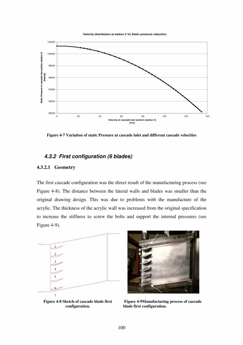
100
Velocity distribution at station 2 Vs Static pressure reduction
90000
92000
94000
96000
98000
100000
102000
0 20 40 60 80 100 120 140
Velocity at cascade test section (station 2)
(m/s)
Sta
tic P
ressu
re in
cascad
e test sectio
n (sta
tio
n 2
)
(P
ascal)
Figure 4-7 Variation of static Pressure at cascade inlet and different cascade velocities
4.3.2 First configuration (6 blades)
4.3.2.1 Geometry
The first cascade configuration was the direct result of the manufacturing process (see
Figure 4-8). The distance between the lateral walls and blades was smaller than the
original drawing design. This was due to problems with the manufacture of the
acrylic. The thickness of the acrylic wall was increased from the original specification
to increase the stiffness to screw the bolts and support the internal pressures (see
Figure 4-9).
Figure 4-8 Sketch of cascade blade first
configuration.
Figure 4-9Manufacturing process of cascade
blade first configuration.
1 2 3 4 5 6 7
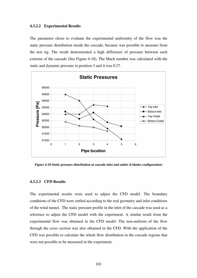
101
4.3.2.2 Experimental Results
The parameter chose to evaluate the experimental uniformity of the flow was the
static pressure distribution inside the cascade, because was possible to measure from
the test rig. The result demonstrated a high difference of pressure between each
extreme of the cascade (See Figure 4-10). The Mach number was calculated with the
static and dynamic pressure in position-3 and it was 0.27.
Static Pressures
91000
91500
92000
92500
93000
93500
94000
94500
95000
0 1 2 3 4 5 6
Pipe location
Pre
ss
ure
[P
a]
Top Inlet
Bottom Inlet
Top Outlet
Bottom Outlet
Figure 4-10 Static pressure distribution at cascade inlet and outlet (6 blades configuration)
4.3.2.3 CFD Results
The experimental results were used to adjust the CFD model. The boundary
conditions of the CFD were settled according to the real geometry and inlet conditions
of the wind tunnel. The static pressure profile in the inlet of the cascade was used as a
reference to adjust the CFD model with the experiment. A similar result from the
experimental flow was obtained in the CFD model. The non-uniform of the flow
through the cross section was also obtained in the CFD. With the application of the
CFD was possible to calculate the whole flow distribution in the cascade regions that
were not possible to be measured in the experiment.
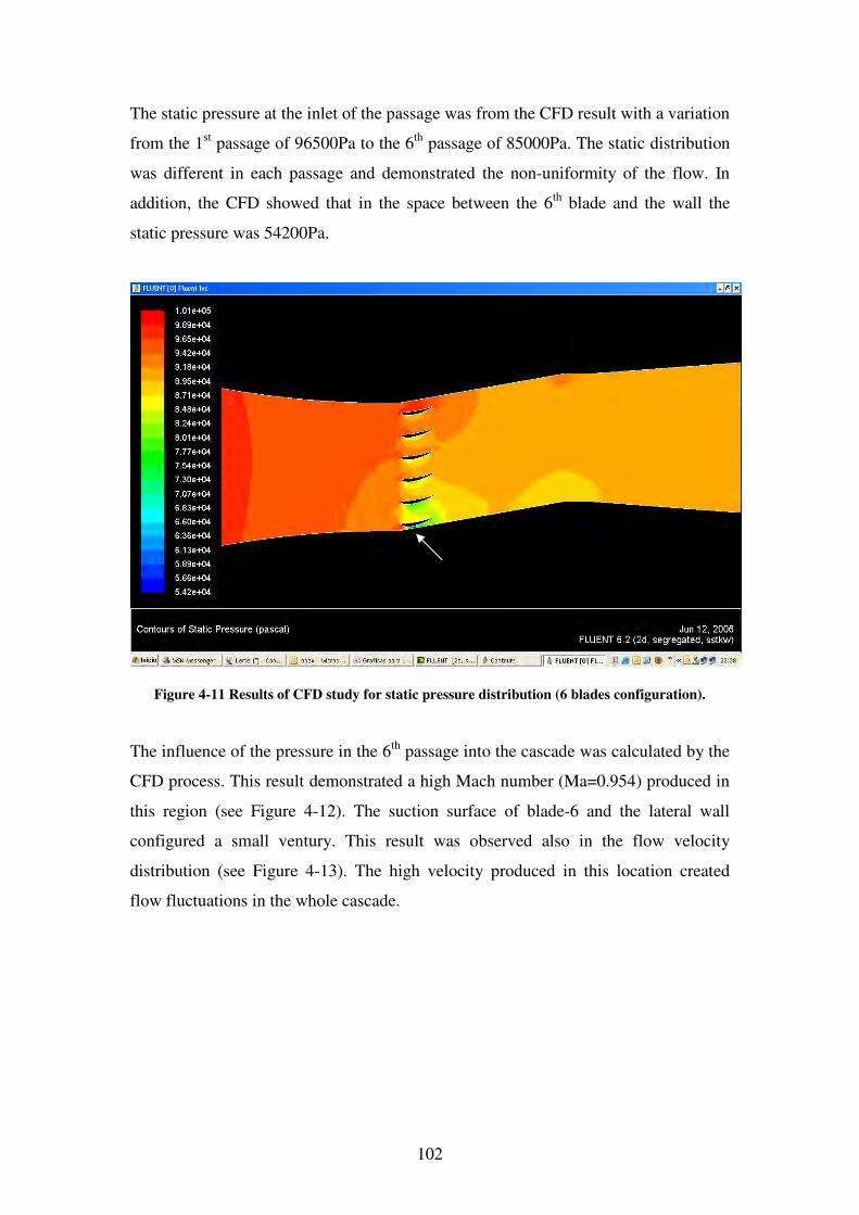
102
The static pressure at the inlet of the passage was from the CFD result with a variation
from the 1st passage of 96500Pa to the 6th passage of 85000Pa. The static distribution
was different in each passage and demonstrated the non-uniformity of the flow. In
addition, the CFD showed that in the space between the 6th blade and the wall the
static pressure was 54200Pa.
Figure 4-11 Results of CFD study for static pressure distribution (6 blades configuration).
The influence of the pressure in the 6th passage into the cascade was calculated by the
CFD process. This result demonstrated a high Mach number (Ma=0.954) produced in
this region (see Figure 4-12). The suction surface of blade-6 and the lateral wall
configured a small ventury. This result was observed also in the flow velocity
distribution (see Figure 4-13). The high velocity produced in this location created
flow fluctuations in the whole cascade.
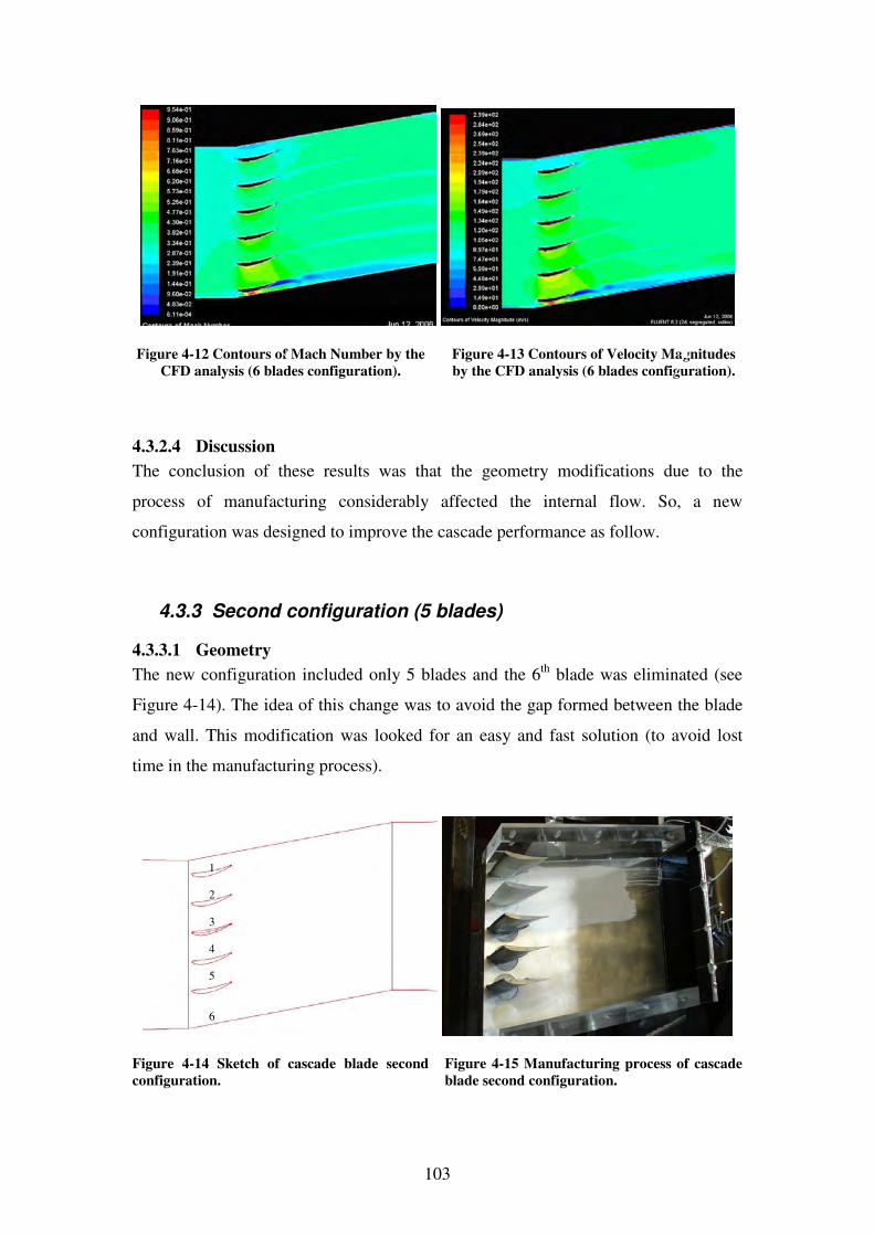
103
Figure 4-12 Contours of Mach Number by the
CFD analysis (6 blades configuration).
Figure 4-13 Contours of Velocity Magnitudes
by the CFD analysis (6 blades configuration).
4.3.2.4 Discussion
The conclusion of these results was that the geometry modifications due to the
process of manufacturing considerably affected the internal flow. So, a new
configuration was designed to improve the cascade performance as follow.
4.3.3 Second configuration (5 blades)
4.3.3.1 Geometry
The new configuration included only 5 blades and the 6th blade was eliminated (see
Figure 4-14). The idea of this change was to avoid the gap formed between the blade
and wall. This modification was looked for an easy and fast solution (to avoid lost
time in the manufacturing process).
Figure 4-14 Sketch of cascade blade second
configuration.
Figure 4-15 Manufacturing process of cascade
blade second configuration.
1 2 3 4 5 6
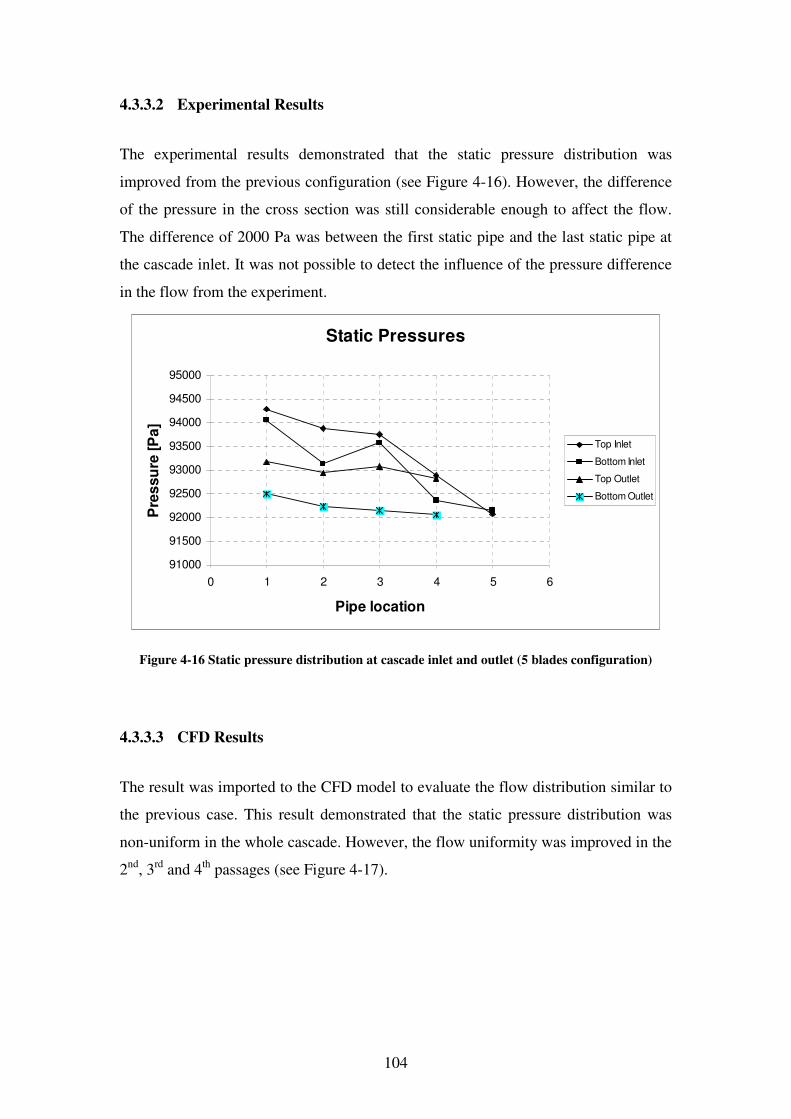
104
4.3.3.2 Experimental Results
The experimental results demonstrated that the static pressure distribution was
improved from the previous configuration (see Figure 4-16). However, the difference
of the pressure in the cross section was still considerable enough to affect the flow.
The difference of 2000 Pa was between the first static pipe and the last static pipe at
the cascade inlet. It was not possible to detect the influence of the pressure difference
in the flow from the experiment.
Static Pressures
91000
91500
92000
92500
93000
93500
94000
94500
95000
0 1 2 3 4 5 6
Pipe location
Pre
ss
ure
[P
a]
Top Inlet
Bottom Inlet
Top Outlet
Bottom Outlet
Figure 4-16 Static pressure distribution at cascade inlet and outlet (5 blades configuration)
4.3.3.3 CFD Results
The result was imported to the CFD model to evaluate the flow distribution similar to
the previous case. This result demonstrated that the static pressure distribution was
non-uniform in the whole cascade. However, the flow uniformity was improved in the
2nd, 3rd and 4th passages (see Figure 4-17).
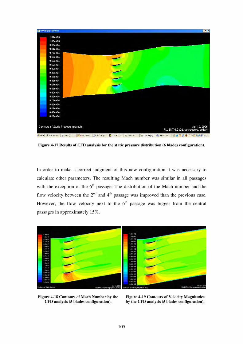
105
Figure 4-17 Results of CFD analysis for the static pressure distribution (6 blades configuration).
In order to make a correct judgment of this new configuration it was necessary to
calculate other parameters. The resulting Mach number was similar in all passages
with the exception of the 6th passage. The distribution of the Mach number and the
flow velocity between the 2nd and 4th passage was improved than the previous case.
However, the flow velocity next to the 6th passage was bigger from the central
passages in approximately 15%.
Figure 4-18 Contours of Mach Number by the
CFD analysis (5 blades configuration).
Figure 4-19 Contours of Velocity Magnitudes
by the CFD analysis (5 blades configuration).
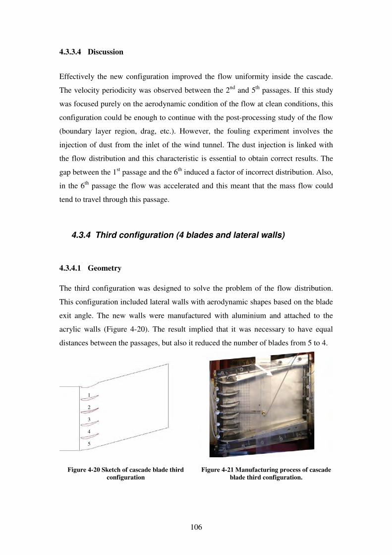
106
4.3.3.4 Discussion
Effectively the new configuration improved the flow uniformity inside the cascade.
The velocity periodicity was observed between the 2nd and 5th passages. If this study
was focused purely on the aerodynamic condition of the flow at clean conditions, this
configuration could be enough to continue with the post-processing study of the flow
(boundary layer region, drag, etc.). However, the fouling experiment involves the
injection of dust from the inlet of the wind tunnel. The dust injection is linked with
the flow distribution and this characteristic is essential to obtain correct results. The
gap between the 1st passage and the 6th induced a factor of incorrect distribution. Also,
in the 6th passage the flow was accelerated and this meant that the mass flow could
tend to travel through this passage.
4.3.4 Third configuration (4 blades and lateral walls)
4.3.4.1 Geometry
The third configuration was designed to solve the problem of the flow distribution.
This configuration included lateral walls with aerodynamic shapes based on the blade
exit angle. The new walls were manufactured with aluminium and attached to the
acrylic walls (Figure 4-20). The result implied that it was necessary to have equal
distances between the passages, but also it reduced the number of blades from 5 to 4.
Figure 4-20 Sketch of cascade blade third
configuration
Figure 4-21 Manufacturing process of cascade
blade third configuration.
1 2 3 4 5
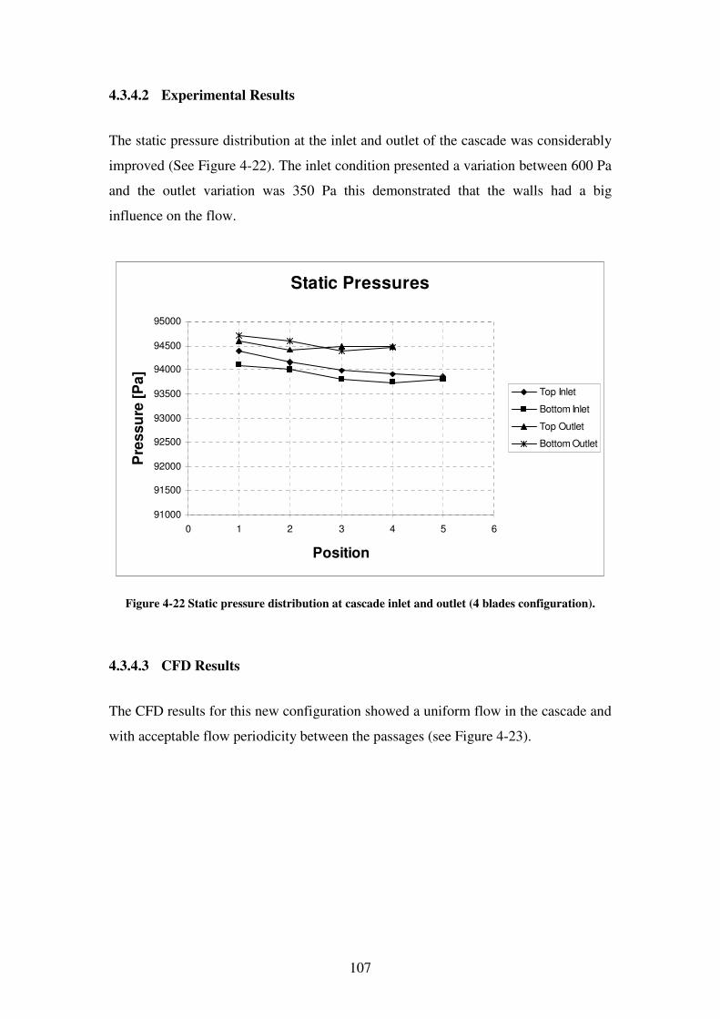
107
4.3.4.2 Experimental Results
The static pressure distribution at the inlet and outlet of the cascade was considerably
improved (See Figure 4-22). The inlet condition presented a variation between 600 Pa
and the outlet variation was 350 Pa this demonstrated that the walls had a big
influence on the flow.
Static Pressures
91000
91500
92000
92500
93000
93500
94000
94500
95000
0 1 2 3 4 5 6
Position
Pre
ss
ure
[P
a]
Top Inlet
Bottom Inlet
Top Outlet
Bottom Outlet
Figure 4-22 Static pressure distribution at cascade inlet and outlet (4 blades configuration).
4.3.4.3 CFD Results
The CFD results for this new configuration showed a uniform flow in the cascade and
with acceptable flow periodicity between the passages (see Figure 4-23).
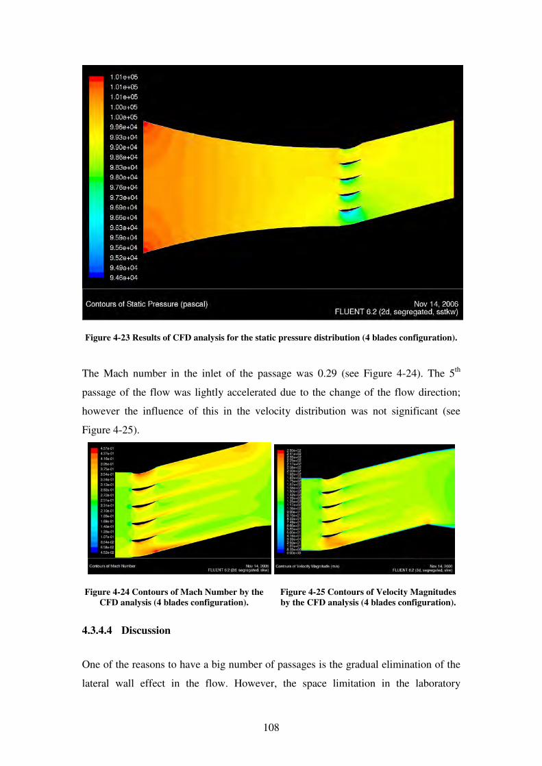
108
Figure 4-23 Results of CFD analysis for the static pressure distribution (4 blades configuration).
The Mach number in the inlet of the passage was 0.29 (see Figure 4-24). The 5th
passage of the flow was lightly accelerated due to the change of the flow direction;
however the influence of this in the velocity distribution was not significant (see
Figure 4-25).
Figure 4-24 Contours of Mach Number by the
CFD analysis (4 blades configuration).
Figure 4-25 Contours of Velocity Magnitudes
by the CFD analysis (4 blades configuration).
4.3.4.4 Discussion
One of the reasons to have a big number of passages is the gradual elimination of the
lateral wall effect in the flow. However, the space limitation in the laboratory
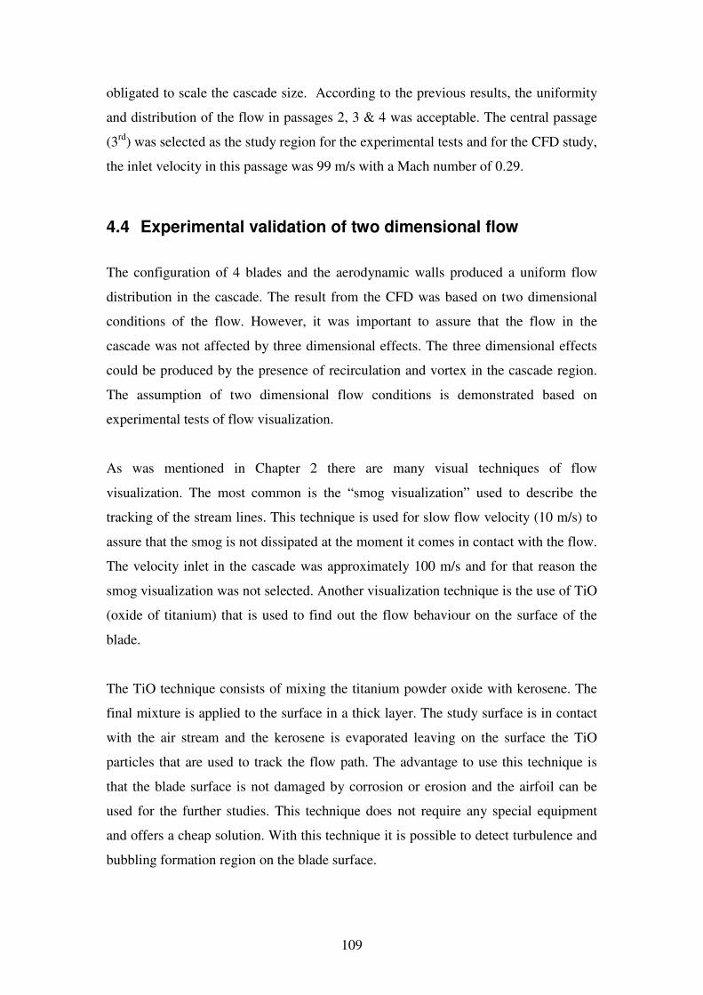
109
obligated to scale the cascade size. According to the previous results, the uniformity
and distribution of the flow in passages 2, 3 & 4 was acceptable. The central passage
(3rd) was selected as the study region for the experimental tests and for the CFD study,
the inlet velocity in this passage was 99 m/s with a Mach number of 0.29.
4.4 Experimental validation of two dimensional flow
The configuration of 4 blades and the aerodynamic walls produced a uniform flow
distribution in the cascade. The result from the CFD was based on two dimensional
conditions of the flow. However, it was important to assure that the flow in the
cascade was not affected by three dimensional effects. The three dimensional effects
could be produced by the presence of recirculation and vortex in the cascade region.
The assumption of two dimensional flow conditions is demonstrated based on
experimental tests of flow visualization.
As was mentioned in Chapter 2 there are many visual techniques of flow
visualization. The most common is the “smog visualization” used to describe the
tracking of the stream lines. This technique is used for slow flow velocity (10 m/s) to
assure that the smog is not dissipated at the moment it comes in contact with the flow.
The velocity inlet in the cascade was approximately 100 m/s and for that reason the
smog visualization was not selected. Another visualization technique is the use of TiO
(oxide of titanium) that is used to find out the flow behaviour on the surface of the
blade.
The TiO technique consists of mixing the titanium powder oxide with kerosene. The
final mixture is applied to the surface in a thick layer. The study surface is in contact
with the air stream and the kerosene is evaporated leaving on the surface the TiO
particles that are used to track the flow path. The advantage to use this technique is
that the blade surface is not damaged by corrosion or erosion and the airfoil can be
used for the further studies. This technique does not require any special equipment
and offers a cheap solution. With this technique it is possible to detect turbulence and
bubbling formation region on the blade surface.
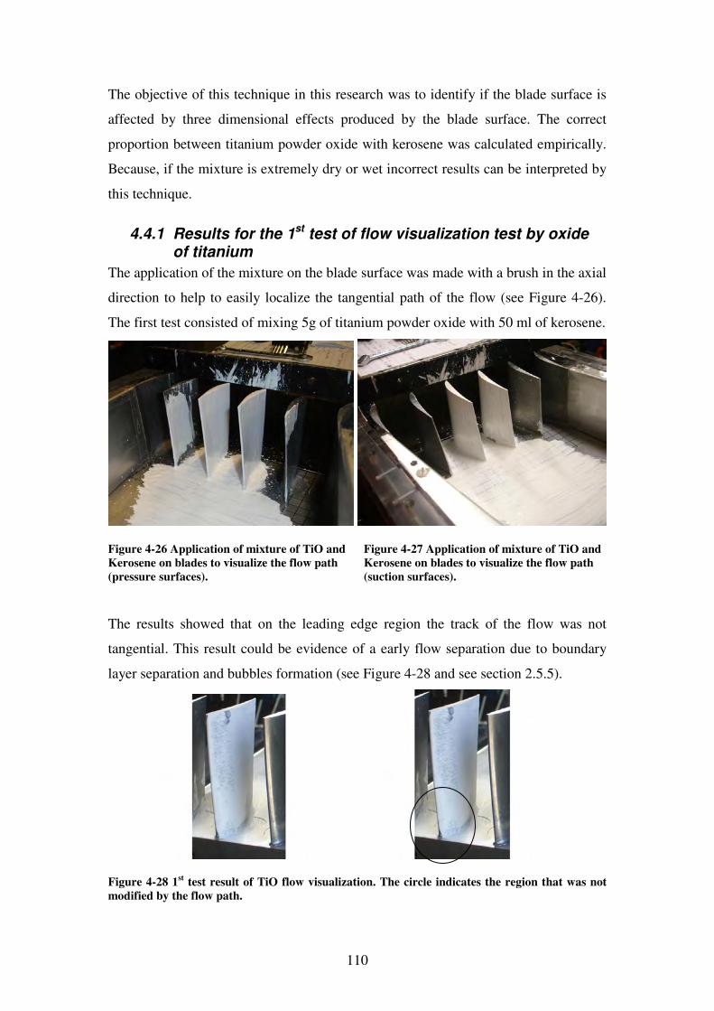
110
The objective of this technique in this research was to identify if the blade surface is
affected by three dimensional effects produced by the blade surface. The correct
proportion between titanium powder oxide with kerosene was calculated empirically.
Because, if the mixture is extremely dry or wet incorrect results can be interpreted by
this technique.
4.4.1 Results for the 1st test of flow visualization test by oxide of titanium
The application of the mixture on the blade surface was made with a brush in the axial
direction to help to easily localize the tangential path of the flow (see Figure 4-26).
The first test consisted of mixing 5g of titanium powder oxide with 50 ml of kerosene.
Figure 4-26 Application of mixture of TiO and
Kerosene on blades to visualize the flow path
(pressure surfaces).
Figure 4-27 Application of mixture of TiO and
Kerosene on blades to visualize the flow path
(suction surfaces).
The results showed that on the leading edge region the track of the flow was not
tangential. This result could be evidence of a early flow separation due to boundary
layer separation and bubbles formation (see Figure 4-28 and see section 2.5.5).
Figure 4-28 1st test result of TiO flow visualization. The circle indicates the region that was not
modified by the flow path.
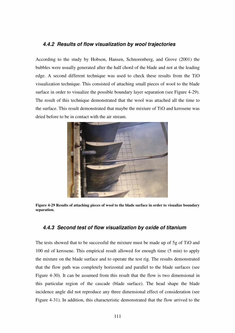
111
4.4.2 Results of flow visualization by wool trajectories
According to the study by Hobson, Hansen, Schnorenberg, and Grove (2001) the
bubbles were usually generated after the half chord of the blade and not at the leading
edge. A second different technique was used to check these results from the TiO
visualization technique. This consisted of attaching small pieces of wool to the blade
surface in order to visualize the possible boundary layer separation (see Figure 4-29).
The result of this technique demonstrated that the wool was attached all the time to
the surface. This result demonstrated that maybe the mixture of TiO and kerosene was
dried before to be in contact with the air stream.
Figure 4-29 Results of attaching pieces of wool to the blade surface in order to visualize boundary
separation.
4.4.3 Second test of flow visualization by oxide of titanium
The tests showed that to be successful the mixture must be made up of 5g of TiO and
100 ml of kerosene. This empirical result allowed for enough time (5 min) to apply
the mixture on the blade surface and to operate the test rig. The results demonstrated
that the flow path was completely horizontal and parallel to the blade surfaces (see
Figure 4-30). It can be assumed from this result that the flow is two dimensional in
this particular region of the cascade (blade surface). The head shape the blade
incidence angle did not reproduce any three dimensional effect of consideration (see
Figure 4-31). In addition, this characteristic demonstrated that the flow arrived to the
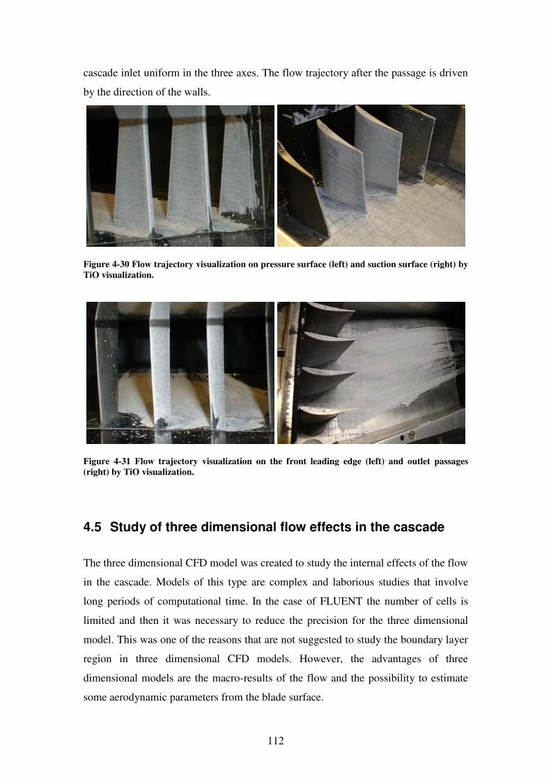
112
cascade inlet uniform in the three axes. The flow trajectory after the passage is driven
by the direction of the walls.
Figure 4-30 Flow trajectory visualization on pressure surface (left) and suction surface (right) by
TiO visualization.
Figure 4-31 Flow trajectory visualization on the front leading edge (left) and outlet passages
(right) by TiO visualization.
4.5 Study of three dimensional flow effects in the cascade
The three dimensional CFD model was created to study the internal effects of the flow
in the cascade. Models of this type are complex and laborious studies that involve
long periods of computational time. In the case of FLUENT the number of cells is
limited and then it was necessary to reduce the precision for the three dimensional
model. This was one of the reasons that are not suggested to study the boundary layer
region in three dimensional CFD models. However, the advantages of three
dimensional models are the macro-results of the flow and the possibility to estimate
some aerodynamic parameters from the blade surface.
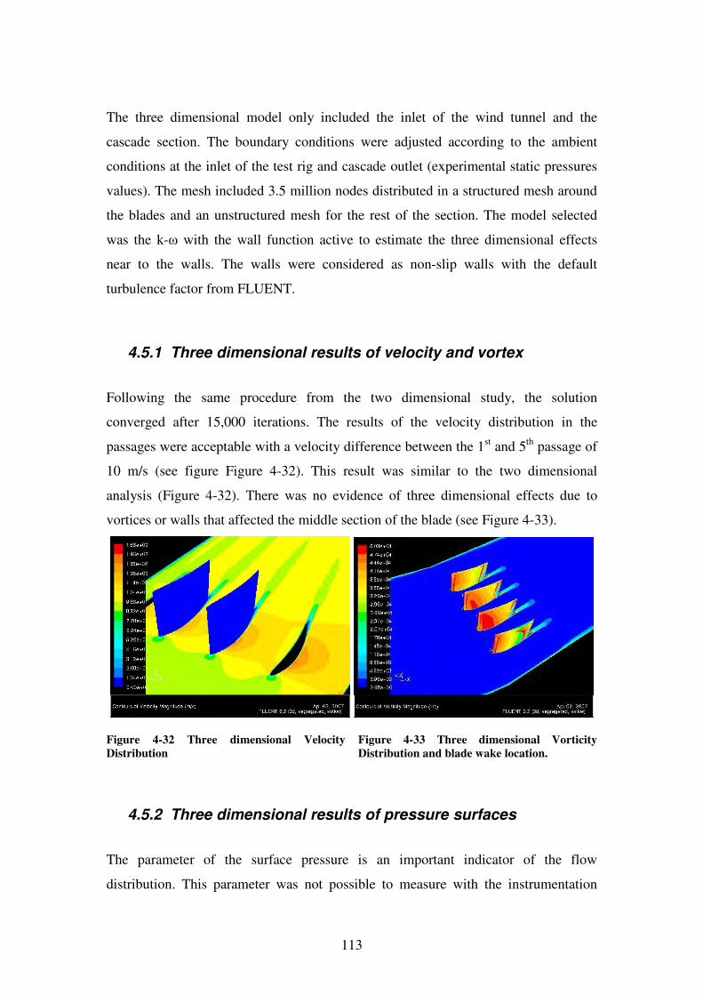
113
The three dimensional model only included the inlet of the wind tunnel and the
cascade section. The boundary conditions were adjusted according to the ambient
conditions at the inlet of the test rig and cascade outlet (experimental static pressures
values). The mesh included 3.5 million nodes distributed in a structured mesh around
the blades and an unstructured mesh for the rest of the section. The model selected
was the k-ω with the wall function active to estimate the three dimensional effects
near to the walls. The walls were considered as non-slip walls with the default
turbulence factor from FLUENT.
4.5.1 Three dimensional results of velocity and vortex
Following the same procedure from the two dimensional study, the solution
converged after 15,000 iterations. The results of the velocity distribution in the
passages were acceptable with a velocity difference between the 1st and 5th passage of
10 m/s (see figure Figure 4-32). This result was similar to the two dimensional
analysis (Figure 4-32). There was no evidence of three dimensional effects due to
vortices or walls that affected the middle section of the blade (see Figure 4-33).
Figure 4-32 Three dimensional Velocity
Distribution
Figure 4-33 Three dimensional Vorticity
Distribution and blade wake location.
4.5.2 Three dimensional results of pressure surfaces
The parameter of the surface pressure is an important indicator of the flow
distribution. This parameter was not possible to measure with the instrumentation
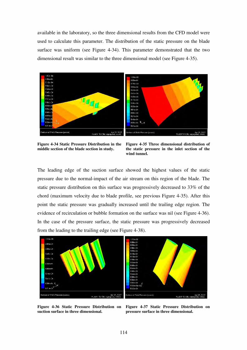
114
available in the laboratory, so the three dimensional results from the CFD model were
used to calculate this parameter. The distribution of the static pressure on the blade
surface was uniform (see Figure 4-34). This parameter demonstrated that the two
dimensional result was similar to the three dimensional model (see Figure 4-35).
Figure 4-34 Static Pressure Distribution in the
middle section of the blade section in study.
Figure 4-35 Three dimensional distribution of
the static pressure in the inlet section of the
wind tunnel.
The leading edge of the suction surface showed the highest values of the static
pressure due to the normal-impact of the air stream on this region of the blade. The
static pressure distribution on this surface was progressively decreased to 33% of the
chord (maximum velocity due to blade profile, see previous Figure 4-35). After this
point the static pressure was gradually increased until the trailing edge region. The
evidence of recirculation or bubble formation on the surface was nil (see Figure 4-36).
In the case of the pressure surface, the static pressure was progressively decreased
from the leading to the trailing edge (see Figure 4-38).
Figure 4-36 Static Pressure Distribution on
suction surface in three dimensional.
Figure 4-37 Static Pressure Distribution on
pressure surface in three dimensional.
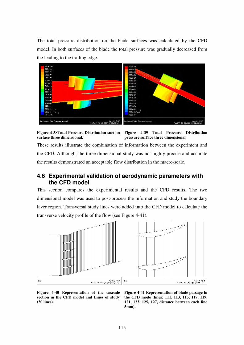
115
The total pressure distribution on the blade surfaces was calculated by the CFD
model. In both surfaces of the blade the total pressure was gradually decreased from
the leading to the trailing edge.
Figure 4-38Total Pressure Distribution suction
surface three dimensional.
Figure 4-39 Total Pressure Distribution
pressure surface three dimensional
These results illustrate the combination of information between the experiment and
the CFD. Although, the three dimensional study was not highly precise and accurate
the results demonstrated an acceptable flow distribution in the macro-scale.
4.6 Experimental validation of aerodynamic parameters with the CFD model
This section compares the experimental results and the CFD results. The two
dimensional model was used to post-process the information and study the boundary
layer region. Transversal study lines were added into the CFD model to calculate the
transverse velocity profile of the flow (see Figure 4-41).
Figure 4-40 Representation of the cascade
section in the CFD model and Lines of study
(30 lines).
Figure 4-41 Representation of blade passage in
the CFD mode (lines: 111, 113, 115, 117, 119,
121, 123, 125, 127, distance between each line
5mm).
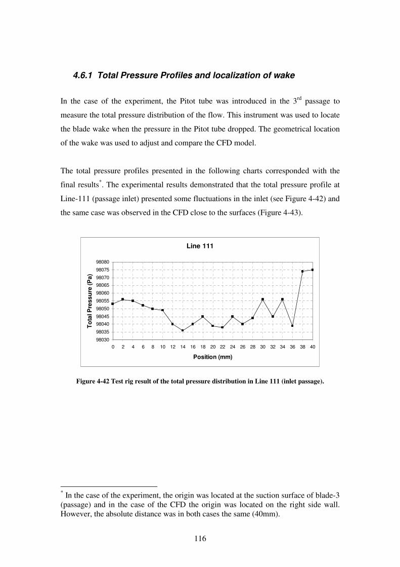
116
4.6.1 Total Pressure Profiles and localization of wake
In the case of the experiment, the Pitot tube was introduced in the 3rd passage to
measure the total pressure distribution of the flow. This instrument was used to locate
the blade wake when the pressure in the Pitot tube dropped. The geometrical location
of the wake was used to adjust and compare the CFD model.
The total pressure profiles presented in the following charts corresponded with the
final results*. The experimental results demonstrated that the total pressure profile at
Line-111 (passage inlet) presented some fluctuations in the inlet (see Figure 4-42) and
the same case was observed in the CFD close to the surfaces (Figure 4-43).
Line 111
98030
98035
98040
98045
98050
98055
98060
98065
98070
98075
98080
0 2 4 6 8 10 12 14 16 18 20 22 24 26 28 30 32 34 36 38 40
Position (mm)
To
tal P
ress
ure
(P
a)
Figure 4-42 Test rig result of the total pressure distribution in Line 111 (inlet passage).
* In the case of the experiment, the origin was located at the suction surface of blade-3 (passage) and in the case of the CFD the origin was located on the right side wall. However, the absolute distance was in both cases the same (40mm).
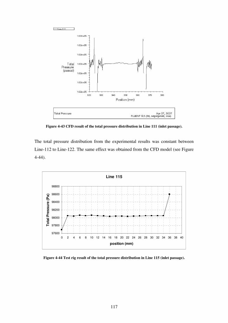
117
Figure 4-43 CFD result of the total pressure distribution in Line 111 (inlet passage).
The total pressure distribution from the experimental results was constant between
Line-112 to Line-122. The same effect was obtained from the CFD model (see Figure
4-44).
Line 115
97600
97800
98000
98200
98400
98600
98800
0 2 4 6 8 10 12 14 16 18 20 22 24 26 28 30 32 34 36 38 40
position (mm)
To
tal P
res
su
re (
Pa
)
Figure 4-44 Test rig result of the total pressure distribution in Line 115 (inlet passage).
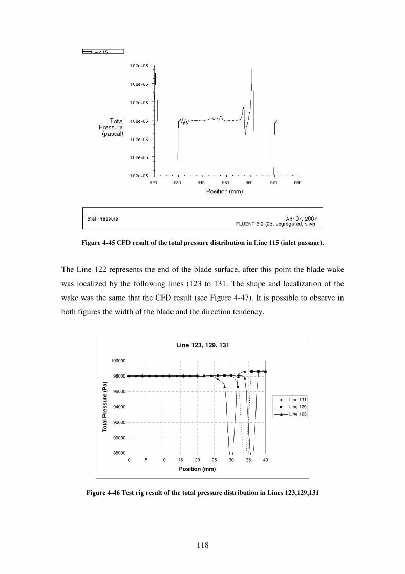
118
Figure 4-45 CFD result of the total pressure distribution in Line 115 (inlet passage).
The Line-122 represents the end of the blade surface, after this point the blade wake
was localized by the following lines (123 to 131. The shape and localization of the
wake was the same that the CFD result (see Figure 4-47). It is possible to observe in
both figures the width of the blade and the direction tendency.
Line 123, 129, 131
88000
90000
92000
94000
96000
98000
100000
0 5 10 15 20 25 30 35 40
Position (mm)
To
tal P
ress
ure
(P
a)
Line 131
Line 129
Line 123
Figure 4-46 Test rig result of the total pressure distribution in Lines 123,129,131
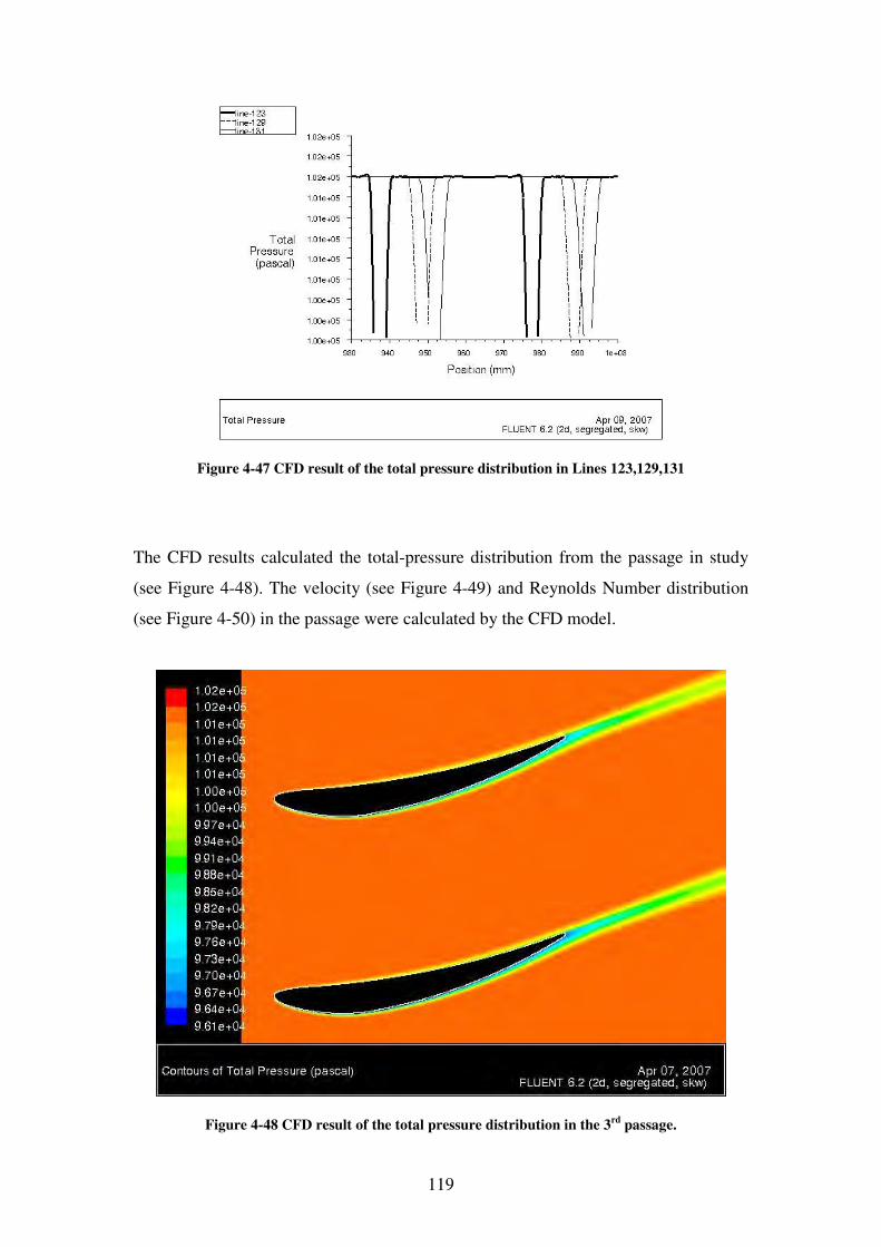
119
Figure 4-47 CFD result of the total pressure distribution in Lines 123,129,131
The CFD results calculated the total-pressure distribution from the passage in study
(see Figure 4-48). The velocity (see Figure 4-49) and Reynolds Number distribution
(see Figure 4-50) in the passage were calculated by the CFD model.
Figure 4-48 CFD result of the total pressure distribution in the 3rd
passage.
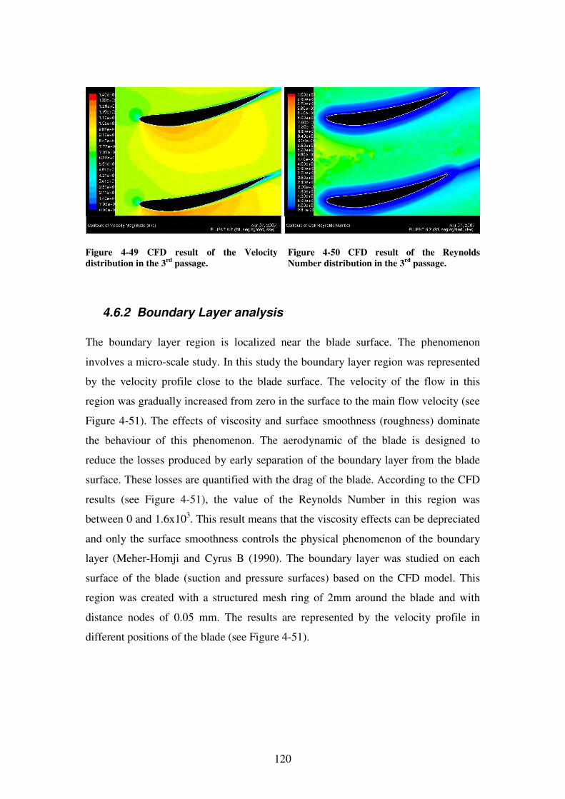
120
Figure 4-49 CFD result of the Velocity
distribution in the 3rd
passage.
Figure 4-50 CFD result of the Reynolds
Number distribution in the 3rd
passage.
4.6.2 Boundary Layer analysis
The boundary layer region is localized near the blade surface. The phenomenon
involves a micro-scale study. In this study the boundary layer region was represented
by the velocity profile close to the blade surface. The velocity of the flow in this
region was gradually increased from zero in the surface to the main flow velocity (see
Figure 4-51). The effects of viscosity and surface smoothness (roughness) dominate
the behaviour of this phenomenon. The aerodynamic of the blade is designed to
reduce the losses produced by early separation of the boundary layer from the blade
surface. These losses are quantified with the drag of the blade. According to the CFD
results (see Figure 4-51), the value of the Reynolds Number in this region was
between 0 and 1.6x10³. This result means that the viscosity effects can be depreciated
and only the surface smoothness controls the physical phenomenon of the boundary
layer (Meher-Homji and Cyrus B (1990). The boundary layer was studied on each
surface of the blade (suction and pressure surfaces) based on the CFD model. This
region was created with a structured mesh ring of 2mm around the blade and with
distance nodes of 0.05 mm. The results are represented by the velocity profile in
different positions of the blade (see Figure 4-51).
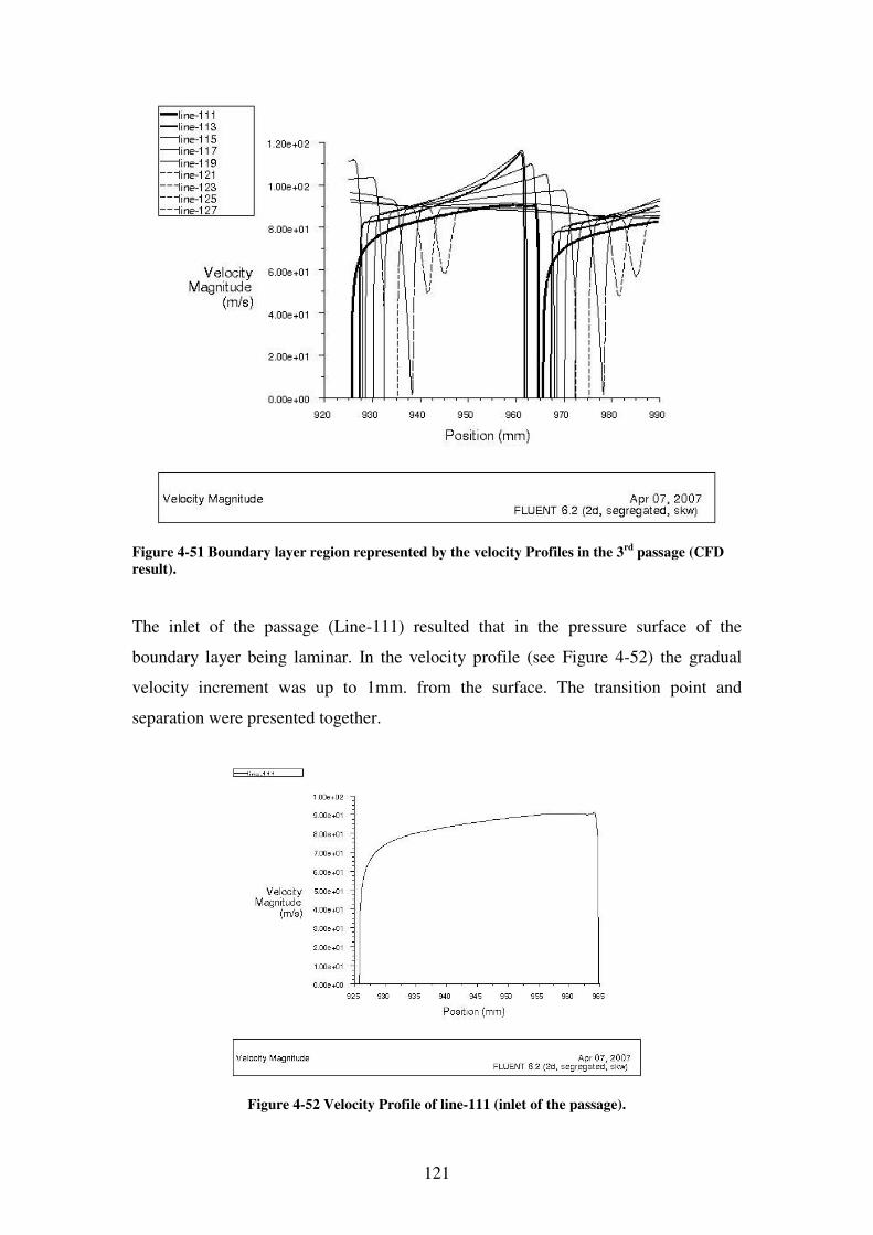
121
Figure 4-51 Boundary layer region represented by the velocity Profiles in the 3rd
passage (CFD
result).
The inlet of the passage (Line-111) resulted that in the pressure surface of the
boundary layer being laminar. In the velocity profile (see Figure 4-52) the gradual
velocity increment was up to 1mm. from the surface. The transition point and
separation were presented together.
Figure 4-52 Velocity Profile of line-111 (inlet of the passage).
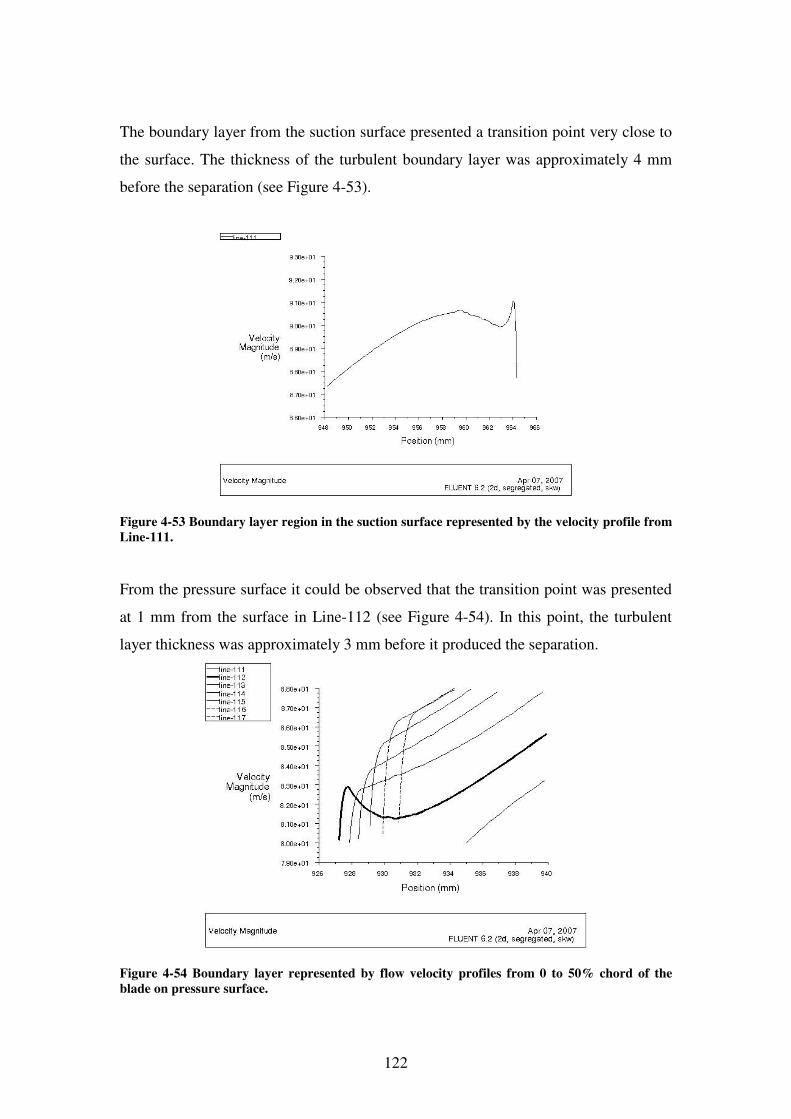
122
The boundary layer from the suction surface presented a transition point very close to
the surface. The thickness of the turbulent boundary layer was approximately 4 mm
before the separation (see Figure 4-53).
Figure 4-53 Boundary layer region in the suction surface represented by the velocity profile from
Line-111.
From the pressure surface it could be observed that the transition point was presented
at 1 mm from the surface in Line-112 (see Figure 4-54). In this point, the turbulent
layer thickness was approximately 3 mm before it produced the separation.
Figure 4-54 Boundary layer represented by flow velocity profiles from 0 to 50% chord of the
blade on pressure surface.
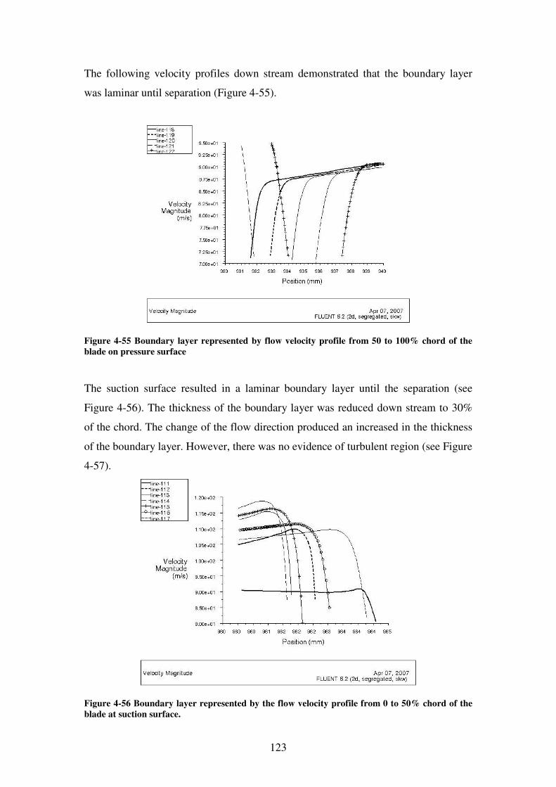
123
The following velocity profiles down stream demonstrated that the boundary layer
was laminar until separation (Figure 4-55).
Figure 4-55 Boundary layer represented by flow velocity profile from 50 to 100% chord of the
blade on pressure surface
The suction surface resulted in a laminar boundary layer until the separation (see
Figure 4-56). The thickness of the boundary layer was reduced down stream to 30%
of the chord. The change of the flow direction produced an increased in the thickness
of the boundary layer. However, there was no evidence of turbulent region (see Figure
4-57).
Figure 4-56 Boundary layer represented by the flow velocity profile from 0 to 50% chord of the
blade at suction surface.
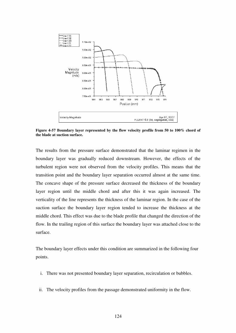
124
Figure 4-57 Boundary layer represented by the flow velocity profile from 50 to 100% chord of
the blade at suction surface.
The results from the pressure surface demonstrated that the laminar regimen in the
boundary layer was gradually reduced downstream. However, the effects of the
turbulent region were not observed from the velocity profiles. This means that the
transition point and the boundary layer separation occurred almost at the same time.
The concave shape of the pressure surface decreased the thickness of the boundary
layer region until the middle chord and after this it was again increased. The
verticality of the line represents the thickness of the laminar region. In the case of the
suction surface the boundary layer region tended to increase the thickness at the
middle chord. This effect was due to the blade profile that changed the direction of the
flow. In the trailing region of this surface the boundary layer was attached close to the
surface.
The boundary layer effects under this condition are summarized in the following four
points.
i. There was not presented boundary layer separation, recirculation or bubbles.
ii. The velocity profiles from the passage demonstrated uniformity in the flow.

125
iii. The middle section of the blade on the surface suction presented a change of
velocity and boundary layer region due to the aerodynamic shape of the blade
and change of direction.
iv. The head of the blade in both surfaces presented changes in the boundary layer
region due to the impact of the air in the blade surface.
126
5 FOULING MODEL
5.1 Introduction
Fouling is one of the most important degradation mechanisms present in gas turbine
compressors. Chapter 2 mentioned that the mechanism of fouling on blades has not
been studied and many unknowns about this phenomenon remain. In this study, the
problem of compressor fouling has been associated with the blade aerodynamics and
gas turbine performance. The particular parameter of the surface roughness has been
selected to measure the fouling.
The information presented in this chapter includes the most important result of this
research. The result of the fouling mechanism was obtained from a preliminary
experimental model. The validation of these experimental results was based on two
sources of information: the results from the CFD study and the information recorded
from industrial engines in operation. As it is going to be presented in this chapter, the
mechanism of fouling was evident. The modification of the blade surface changed the
blade aerodynamics.
This chapter is divided into four sections. The first section includes information about
the real operation of industrial gas turbines in order to know the conditions to
reproduce in the test rig. The second section presents the design of the fouling system.
The third section shows the experimental results from the fouling process on the
blades. The last section summarizes the results in a first approach mathematical model
to describe the fouling mechanism. In this last section is presented the study of the
boundary layer under fouling conditions.
5.2 Preliminary experimental conditions
The fouling system was designed with the assumption that the flow travels uniform
inside the cascade. It was assumed that the dust particles mixed with the air in a
uniform manner. However, in the real application this distribution of the dust in the
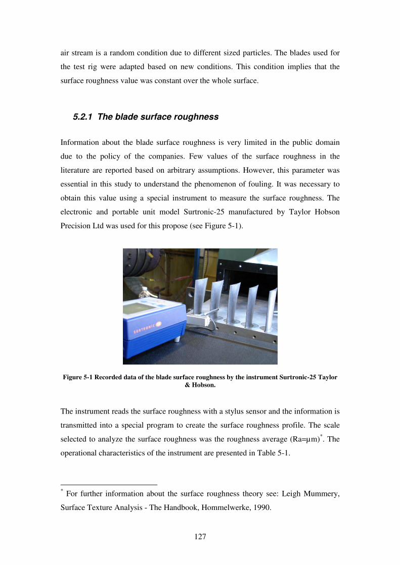
127
air stream is a random condition due to different sized particles. The blades used for
the test rig were adapted based on new conditions. This condition implies that the
surface roughness value was constant over the whole surface.
5.2.1 The blade surface roughness
Information about the blade surface roughness is very limited in the public domain
due to the policy of the companies. Few values of the surface roughness in the
literature are reported based on arbitrary assumptions. However, this parameter was
essential in this study to understand the phenomenon of fouling. It was necessary to
obtain this value using a special instrument to measure the surface roughness. The
electronic and portable unit model Surtronic-25 manufactured by Taylor Hobson
Precision Ltd was used for this propose (see Figure 5-1).
Figure 5-1 Recorded data of the blade surface roughness by the instrument Surtronic-25 Taylor
& Hobson.
The instrument reads the surface roughness with a stylus sensor and the information is
transmitted into a special program to create the surface roughness profile. The scale
selected to analyze the surface roughness was the roughness average (Ra=µm)*. The
operational characteristics of the instrument are presented in Table 5-1.
* For further information about the surface roughness theory see: Leigh Mummery,
Surface Texture Analysis - The Handbook, Hommelwerke, 1990.
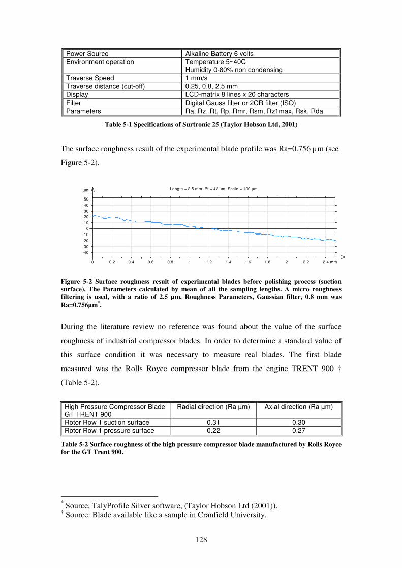
128
Power Source Alkaline Battery 6 volts
Environment operation Temperature 5~40C Humidity 0-80% non condensing
Traverse Speed 1 mm/s
Traverse distance (cut-off) 0.25, 0.8, 2.5 mm
Display LCD-matrix 8 lines x 20 characters
Filter Digital Gauss filter or 2CR filter (ISO)
Parameters Ra, Rz, Rt, Rp, Rmr, Rsm, Rz1max, Rsk, Rda
Table 5-1 Specifications of Surtronic 25 (Taylor Hobson Ltd, 2001)
The surface roughness result of the experimental blade profile was Ra=0.756 µm (see
Figure 5-2).
µm
-40
-30
-20
-10
0
10
20
30
40
50
0 0.2 0.4 0.6 0.8 1 1.2 1.4 1.6 1.8 2 2.2 2.4 mm
Length = 2.5 mm Pt = 42 µm Scale = 100 µm
Figure 5-2 Surface roughness result of experimental blades before polishing process (suction
surface). The Parameters calculated by mean of all the sampling lengths. A micro roughness
filtering is used, with a ratio of 2.5 µm. Roughness Parameters, Gaussian filter, 0.8 mm was
Ra=0.756µm*.
During the literature review no reference was found about the value of the surface
roughness of industrial compressor blades. In order to determine a standard value of
this surface condition it was necessary to measure real blades. The first blade
measured was the Rolls Royce compressor blade from the engine TRENT 900 †
(Table 5-2).
High Pressure Compressor Blade GT TRENT 900
Radial direction (Ra µm) Axial direction (Ra µm)
Rotor Row 1 suction surface 0.31 0.30
Rotor Row 1 pressure surface 0.22 0.27
Table 5-2 Surface roughness of the high pressure compressor blade manufactured by Rolls Royce
for the GT Trent 900.
* Source, TalyProfile Silver software, (Taylor Hobson Ltd (2001)). † Source: Blade available like a sample in Cranfield University.
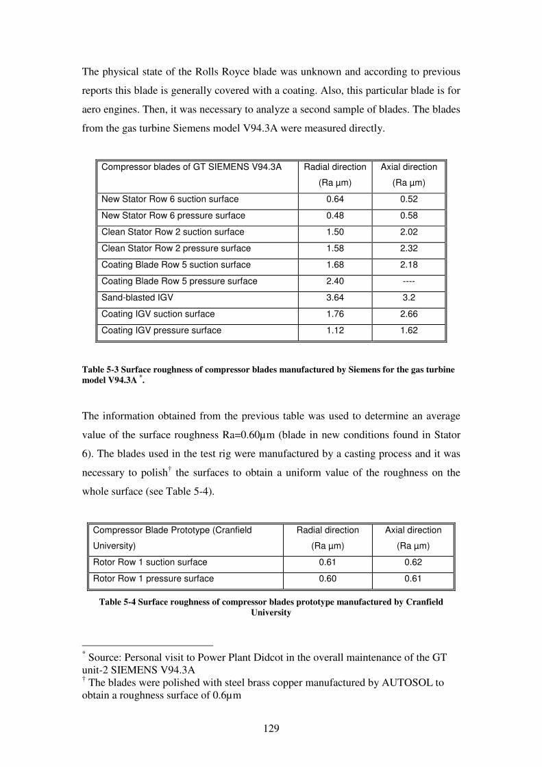
129
The physical state of the Rolls Royce blade was unknown and according to previous
reports this blade is generally covered with a coating. Also, this particular blade is for
aero engines. Then, it was necessary to analyze a second sample of blades. The blades
from the gas turbine Siemens model V94.3A were measured directly.
Compressor blades of GT SIEMENS V94.3A Radial direction
(Ra µm)
Axial direction
(Ra µm)
New Stator Row 6 suction surface 0.64 0.52
New Stator Row 6 pressure surface 0.48 0.58
Clean Stator Row 2 suction surface 1.50 2.02
Clean Stator Row 2 pressure surface 1.58 2.32
Coating Blade Row 5 suction surface 1.68 2.18
Coating Blade Row 5 pressure surface 2.40 ----
Sand-blasted IGV 3.64 3.2
Coating IGV suction surface 1.76 2.66
Coating IGV pressure surface 1.12 1.62
Table 5-3 Surface roughness of compressor blades manufactured by Siemens for the gas turbine
model V94.3A *.
The information obtained from the previous table was used to determine an average
value of the surface roughness Ra=0.60µm (blade in new conditions found in Stator
6). The blades used in the test rig were manufactured by a casting process and it was
necessary to polish† the surfaces to obtain a uniform value of the roughness on the
whole surface (see Table 5-4).
Compressor Blade Prototype (Cranfield
University)
Radial direction
(Ra µm)
Axial direction
(Ra µm)
Rotor Row 1 suction surface 0.61 0.62
Rotor Row 1 pressure surface 0.60 0.61
Table 5-4 Surface roughness of compressor blades prototype manufactured by Cranfield
University
* Source: Personal visit to Power Plant Didcot in the overall maintenance of the GT unit-2 SIEMENS V94.3A † The blades were polished with steel brass copper manufactured by AUTOSOL to obtain a roughness surface of 0.6µm
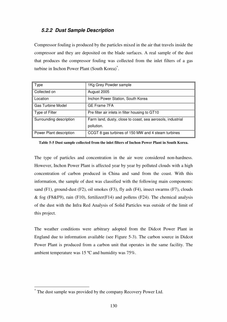
130
5.2.2 Dust Sample Description
Compressor fouling is produced by the particles mixed in the air that travels inside the
compressor and they are deposited on the blade surfaces. A real sample of the dust
that produces the compressor fouling was collected from the inlet filters of a gas
turbine in Inchon Power Plant (South Korea)*.
Type 1Kg Grey Powder sample
Collected on August 2005
Location Inchon Power Station, South Korea
Gas Turbine Model GE Frame 7FA
Type of Filter Pre filter air inlets in filter housing to GT10
Surrounding description Farm land, dusty, close to coast, sea aerosols, industrial
pollution.
Power Plant description CCGT 8 gas turbines of 150 MW and 4 steam turbines
Table 5-5 Dust sample collected from the inlet filters of Inchon Power Plant in South Korea.
The type of particles and concentration in the air were considered non-hardness.
However, Inchon Power Plant is affected year by year by polluted clouds with a high
concentration of carbon produced in China and sand from the coast. With this
information, the sample of dust was classified with the following main components:
sand (F1), ground-dust (F2), oil smokes (F3), fly ash (F4), insect swarms (F7), clouds
& fog (F8&F9), rain (F10), fertilizer(F14) and pollens (F24). The chemical analysis
of the dust with the Infra Red Analysis of Solid Particles was outside of the limit of
this project.
The weather conditions were arbitrary adopted from the Didcot Power Plant in
England due to information available (see Figure 5-3). The carbon source in Didcot
Power Plant is produced from a carbon unit that operates in the same facility. The
ambient temperature was 15 ºC and humidity was 75%.
* The dust sample was provided by the company Recovery Power Ltd.

131
Figure 5-3 Inchon Power Plant, South Korea (left), Didcot Power Plant, England UK (right)
5.3 Design of Fouling Injection System
There are many techniques available in the market to mix solid particles into the air
stream. The most advanced technologies are used to transport chemical powder
products such as detergents, paints, etc. It is common to find powder extractors in the
trimmer and metal industries. However, these types of equipment are expensive and
destined to transport large quantities of the product. The idea behind the fouling
system in this experiment was to find an economic alternative which could be used to
transport small quantities of particles. The design of the system was based on the
sand-clock function and assisted with the pressure difference produced in the wind
tunnel inlet.
5.3.1 Sections of the fouling injection system
The system included three sections:
1. Container to keep the dust powder
2. Hose to transport and deliver the powder into the air stream
3. Bracket to adjust the position of the injection point
The Container was a plastic cylinder graduated according to the dust sample weight in
grams. The base of the cylinder was configured with an outlet-cone to control the pass
of particles (similar to the sand-clock). The hose was connected to the outlet-cone to
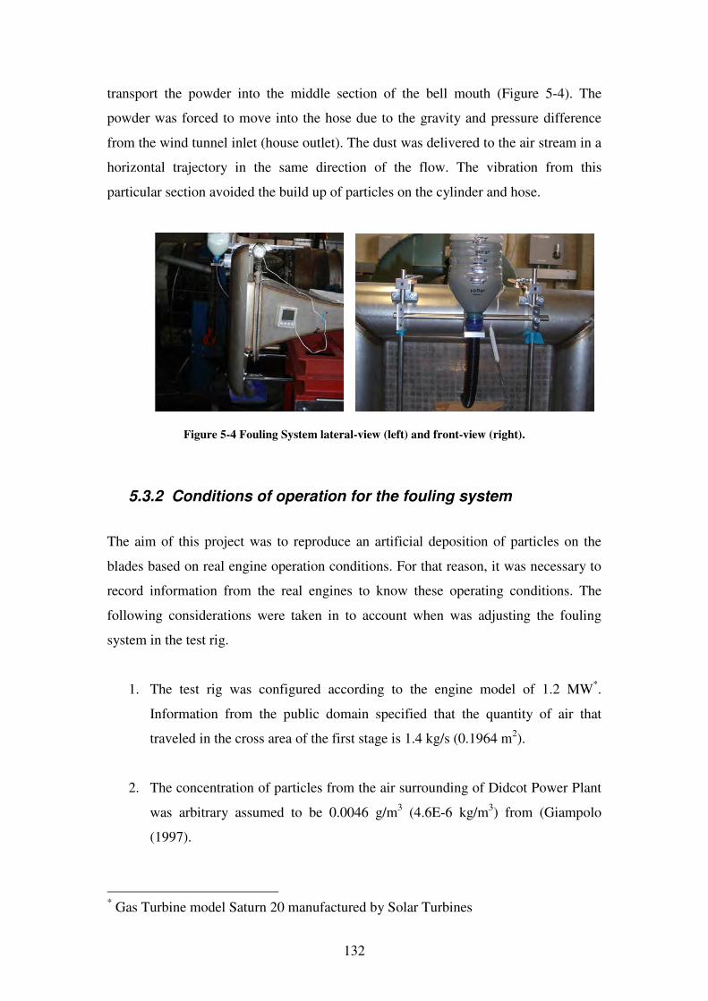
132
transport the powder into the middle section of the bell mouth (Figure 5-4). The
powder was forced to move into the hose due to the gravity and pressure difference
from the wind tunnel inlet (house outlet). The dust was delivered to the air stream in a
horizontal trajectory in the same direction of the flow. The vibration from this
particular section avoided the build up of particles on the cylinder and hose.
Figure 5-4 Fouling System lateral-view (left) and front-view (right).
5.3.2 Conditions of operation for the fouling system
The aim of this project was to reproduce an artificial deposition of particles on the
blades based on real engine operation conditions. For that reason, it was necessary to
record information from the real engines to know these operating conditions. The
following considerations were taken in to account when was adjusting the fouling
system in the test rig.
1. The test rig was configured according to the engine model of 1.2 MW*.
Information from the public domain specified that the quantity of air that
traveled in the cross area of the first stage is 1.4 kg/s (0.1964 m2).
2. The concentration of particles from the air surrounding of Didcot Power Plant
was arbitrary assumed to be 0.0046 g/m3 (4.6E-6 kg/m3) from (Giampolo
(1997).
* Gas Turbine model Saturn 20 manufactured by Solar Turbines
133
3. The engine model of Didcot Power Plant was the engine of 240MW*,
according to the public information this engine operates with a mass flow of
640 kg/s.
4. The filtration system was assumed to have an arbitrary efficiency of 90%
(middle life).
Under these conditions the rate from the dust injection was calculated as follows.
• For the gas turbine of 240MW
Engine volume flow: air
WV
ρ= =528 m3/s
Equation 5-1
where: V = Volume flow
W = Air Mass Flow (640 kg/s)
airρ =1.21 kg/m3
If filterη =90% and the airfoulinionConcentrat /1 = 4.6E-6 kg/m3, then
concentration of particles after filtration was:
airfoulingfilterairfouling ionConcentrationConcentrat // 1)1(2 ×−= η =4.6E-7 kg/m3
The rate of particles mixed in the air inside the compressor was:
airfoulingfouling ionConcentratVRate /2×= =2.433E-4 kg/s = 875.9 g/hr
• For the gas turbine of 1.2MW
The volume flow of this engine was: air
WV
ρ= =5.502 m3/s
where: V = Volume flow
W = Air Mass Flow (6.2 kg/s)
If filterη =90% and the airfoulinionConcentrat /1 = 4.6E-6 kg/m3, then concentration of
particles after filtration was:
* Gas Turbine model V94.3A manufactured by SIEMENS
134
airfoulingfilterairfouling ionConcentrationConcentrat // 1)1(2 ×−= η =4.6E-7 kg/m3
The rate of dust inside the compressor was:
airfoulingfouling ionConcentratVRate /2×= =3.45E-6 kg/s=12.42g/hr
The mass flow of the test rig was 1.4 kg/s equivalent to 22.58% of the total mass flow
from the gas turbine of 1.2MW. Assuming this factor is correct, the results of the
fouling rate are presented in Table 5-6.
Fouling Rate (mass/time) GT 240MW GT 1.2MW Test Rig
g/second 0.2433 0.00345 0.000779
g/minute 14.59 0.207 0.0467406
g/hour 875.9 12.42 2.80
g/day 21,021 298 67.2884
g/week 147,147 2,087 471.24
g/month 4,414,435 9,240 2,086
g/year 52,973,222 110,880 25,036
g/overall maintenance
(4years)
211,892,889 443,520 100,146
Table 5-6 Ideal scenarios of fouling rate for the Siemens V94.3A, Saturn 20 and Test Rig.
The quantity of the dust sample available was 700g. According to the results of the
fouling rate (2.8g/h) this is equivalent to 10 days of continuous operation from the
real engine.
5.4 Experimental results of fouling
The fouling system was tested in the experiment to evaluate the dust deposition
according to information from the real compressor fouling. The information used to
evaluate and validate the dust deposition was based on the fouling presented in the
engine of Didcot Power Plant. Previous experiments were tested in the test rig with an
artificial sample (Flour) to specify the operation condition of the fouling system.
i. Injection of artificial sample (flour powder)
ii. Injection of artificial sample (flour powder) with an artificial glue agent-1
(liquid oil UW40)
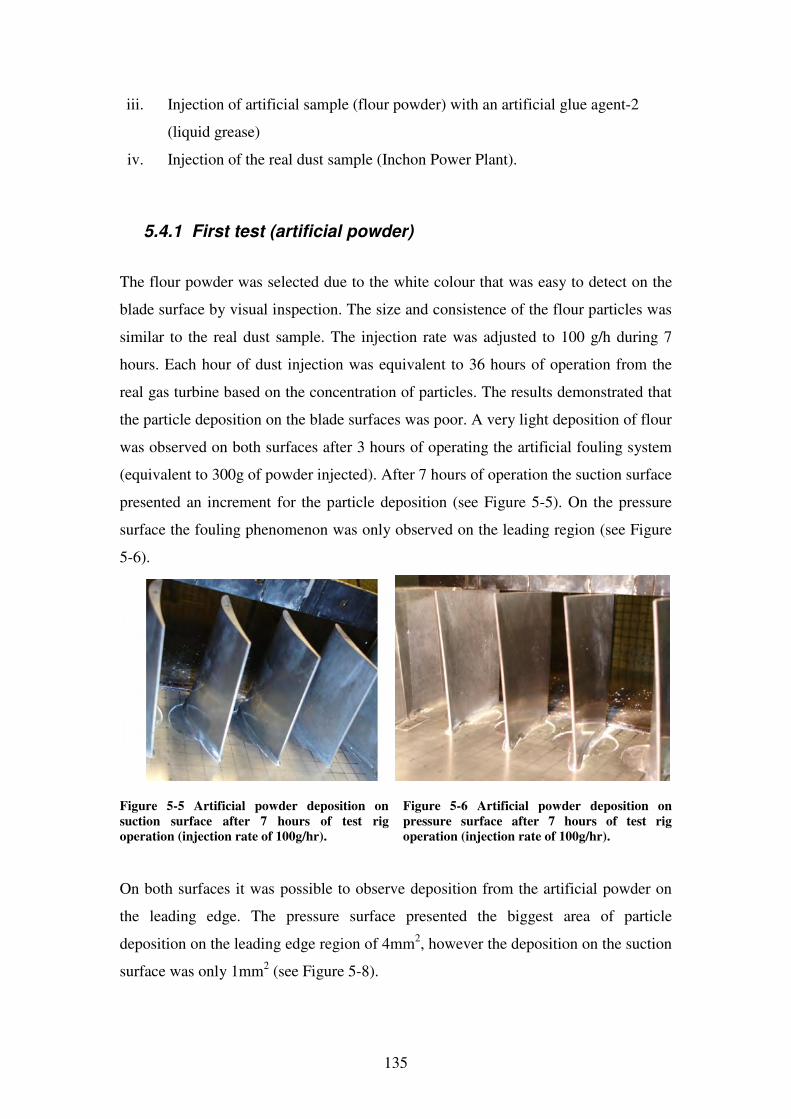
135
iii. Injection of artificial sample (flour powder) with an artificial glue agent-2
(liquid grease)
iv. Injection of the real dust sample (Inchon Power Plant).
5.4.1 First test (artificial powder)
The flour powder was selected due to the white colour that was easy to detect on the
blade surface by visual inspection. The size and consistence of the flour particles was
similar to the real dust sample. The injection rate was adjusted to 100 g/h during 7
hours. Each hour of dust injection was equivalent to 36 hours of operation from the
real gas turbine based on the concentration of particles. The results demonstrated that
the particle deposition on the blade surfaces was poor. A very light deposition of flour
was observed on both surfaces after 3 hours of operating the artificial fouling system
(equivalent to 300g of powder injected). After 7 hours of operation the suction surface
presented an increment for the particle deposition (see Figure 5-5). On the pressure
surface the fouling phenomenon was only observed on the leading region (see Figure
5-6).
Figure 5-5 Artificial powder deposition on
suction surface after 7 hours of test rig
operation (injection rate of 100g/hr).
Figure 5-6 Artificial powder deposition on
pressure surface after 7 hours of test rig
operation (injection rate of 100g/hr).
On both surfaces it was possible to observe deposition from the artificial powder on
the leading edge. The pressure surface presented the biggest area of particle
deposition on the leading edge region of 4mm2, however the deposition on the suction
surface was only 1mm2 (see Figure 5-8).
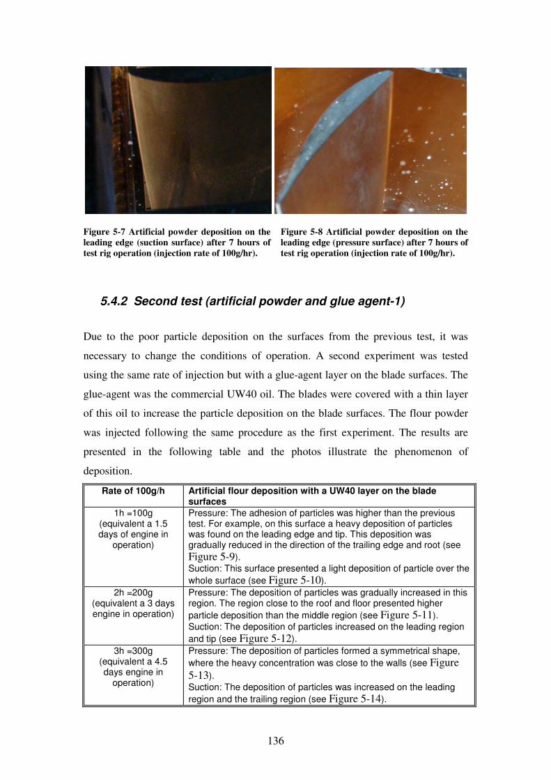
136
Figure 5-7 Artificial powder deposition on the
leading edge (suction surface) after 7 hours of
test rig operation (injection rate of 100g/hr).
Figure 5-8 Artificial powder deposition on the
leading edge (pressure surface) after 7 hours of
test rig operation (injection rate of 100g/hr).
5.4.2 Second test (artificial powder and glue agent-1)
Due to the poor particle deposition on the surfaces from the previous test, it was
necessary to change the conditions of operation. A second experiment was tested
using the same rate of injection but with a glue-agent layer on the blade surfaces. The
glue-agent was the commercial UW40 oil. The blades were covered with a thin layer
of this oil to increase the particle deposition on the blade surfaces. The flour powder
was injected following the same procedure as the first experiment. The results are
presented in the following table and the photos illustrate the phenomenon of
deposition.
Rate of 100g/h Artificial flour deposition with a UW40 layer on the blade surfaces
1h =100g (equivalent a 1.5 days of engine in
operation)
Pressure: The adhesion of particles was higher than the previous test. For example, on this surface a heavy deposition of particles was found on the leading edge and tip. This deposition was gradually reduced in the direction of the trailing edge and root (see
Figure 5-9).
Suction: This surface presented a light deposition of particle over the
whole surface (see Figure 5-10).
2h =200g (equivalent a 3 days engine in operation)
Pressure: The deposition of particles was gradually increased in this region. The region close to the roof and floor presented higher
particle deposition than the middle region (see Figure 5-11).
Suction: The deposition of particles increased on the leading region
and tip (see Figure 5-12).
3h =300g (equivalent a 4.5 days engine in
operation)
Pressure: The deposition of particles formed a symmetrical shape,
where the heavy concentration was close to the walls (see Figure 5-13).
Suction: The deposition of particles was increased on the leading
region and the trailing region (see Figure 5-14).
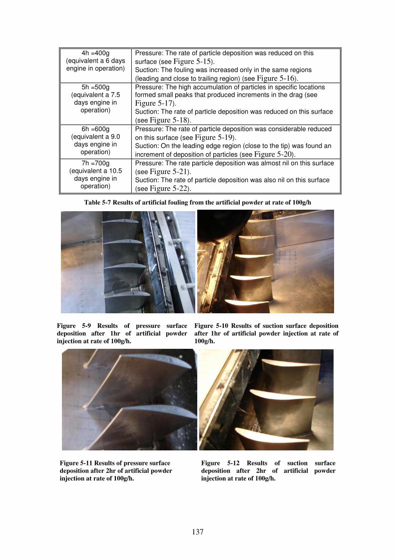
137
4h =400g (equivalent a 6 days engine in operation)
Pressure: The rate of particle deposition was reduced on this
surface (see Figure 5-15).
Suction: The fouling was increased only in the same regions
(leading and close to trailing region) (see Figure 5-16).
5h =500g (equivalent a 7.5 days engine in
operation)
Pressure: The high accumulation of particles in specific locations formed small peaks that produced increments in the drag (see
Figure 5-17).
Suction: The rate of particle deposition was reduced on this surface
(see Figure 5-18).
6h =600g (equivalent a 9.0 days engine in
operation)
Pressure: The rate of particle deposition was considerable reduced
on this surface (see Figure 5-19).
Suction: On the leading edge region (close to the tip) was found an
increment of deposition of particles (see Figure 5-20).
7h =700g (equivalent a 10.5
days engine in operation)
Pressure: The rate particle deposition was almost nil on this surface
(see Figure 5-21).
Suction: The rate of particle deposition was also nil on this surface
(see Figure 5-22).
Table 5-7 Results of artificial fouling from the artificial powder at rate of 100g/h
Figure 5-9 Results of pressure surface
deposition after 1hr of artificial powder
injection at rate of 100g/h.
Figure 5-10 Results of suction surface deposition
after 1hr of artificial powder injection at rate of
100g/h.
Figure 5-11 Results of pressure surface
deposition after 2hr of artificial powder
injection at rate of 100g/h.
Figure 5-12 Results of suction surface
deposition after 2hr of artificial powder
injection at rate of 100g/h.
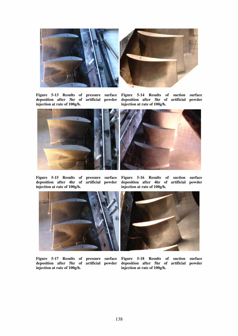
138
Figure 5-13 Results of pressure surface
deposition after 3hr of artificial powder
injection at rate of 100g/h.
Figure 5-14 Results of suction surface
deposition after 3hr of artificial powder
injection at rate of 100g/h.
Figure 5-15 Results of pressure surface
deposition after 4hr of artificial powder
injection at rate of 100g/h.
Figure 5-16 Results of suction surface
deposition after 4hr of artificial powder
injection at rate of 100g/h.
Figure 5-17 Results of pressure surface
deposition after 5hr of artificial powder
injection at rate of 100g/h.
Figure 5-18 Results of suction surface
deposition after 5hr of artificial powder
injection at rate of 100g/h.
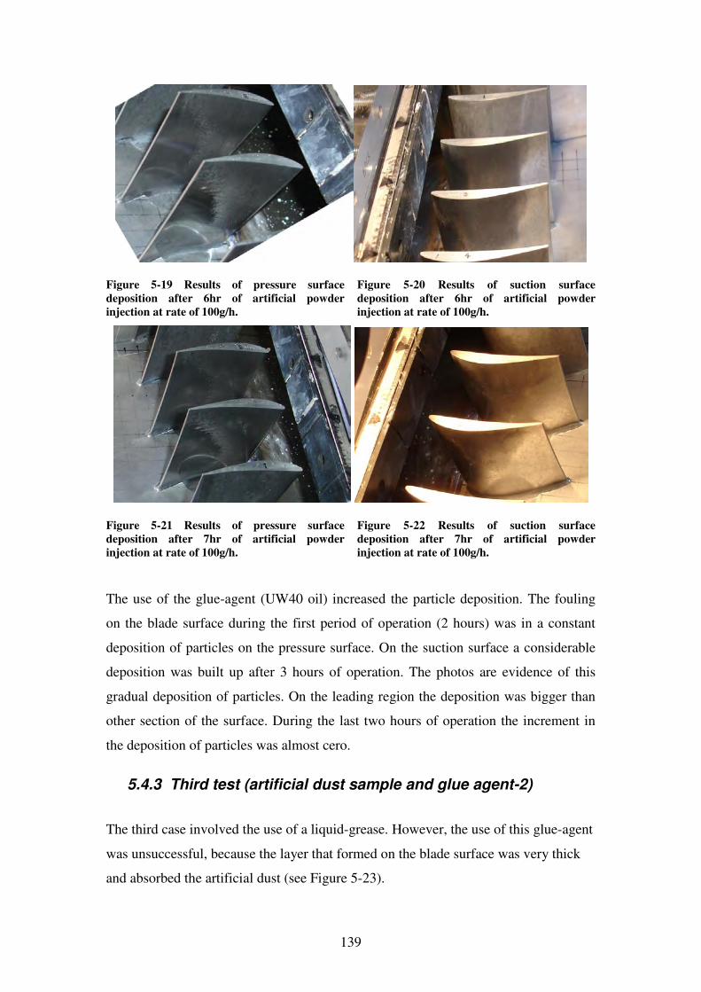
139
Figure 5-19 Results of pressure surface
deposition after 6hr of artificial powder
injection at rate of 100g/h.
Figure 5-20 Results of suction surface
deposition after 6hr of artificial powder
injection at rate of 100g/h.
Figure 5-21 Results of pressure surface
deposition after 7hr of artificial powder
injection at rate of 100g/h.
Figure 5-22 Results of suction surface
deposition after 7hr of artificial powder
injection at rate of 100g/h.
The use of the glue-agent (UW40 oil) increased the particle deposition. The fouling
on the blade surface during the first period of operation (2 hours) was in a constant
deposition of particles on the pressure surface. On the suction surface a considerable
deposition was built up after 3 hours of operation. The photos are evidence of this
gradual deposition of particles. On the leading region the deposition was bigger than
other section of the surface. During the last two hours of operation the increment in
the deposition of particles was almost cero.
5.4.3 Third test (artificial dust sample and glue agent-2)
The third case involved the use of a liquid-grease. However, the use of this glue-agent
was unsuccessful, because the layer that formed on the blade surface was very thick
and absorbed the artificial dust (see Figure 5-23).
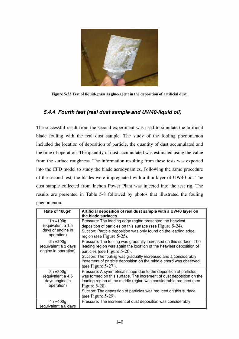
140
Figure 5-23 Test of liquid-grass as glue-agent in the deposition of artificial dust.
5.4.4 Fourth test (real dust sample and UW40-liquid oil)
The successful result from the second experiment was used to simulate the artificial
blade fouling with the real dust sample. The study of the fouling phenomenon
included the location of deposition of particle, the quantity of dust accumulated and
the time of operation. The quantity of dust accumulated was estimated using the value
from the surface roughness. The information resulting from these tests was exported
into the CFD model to study the blade aerodynamics. Following the same procedure
of the second test, the blades were impregnated with a thin layer of UW40 oil. The
dust sample collected from Inchon Power Plant was injected into the test rig. The
results are presented in Table 5-8 followed by photos that illustrated the fouling
phenomenon.
Rate of 100g/h Artificial deposition of real dust sample with a UW40 layer on the blade surfaces
1h =100g (equivalent a 1.5 days of engine in
operation)
Pressure: The leading edge region presented the heaviest
deposition of particles on this surface (see Figure 5-24).
Suction: Particle deposition was only found on the leading edge
region (see Figure 5-25).
2h =200g (equivalent a 3 days engine in operation)
Pressure: The fouling was gradually increased on this surface. The leading region was again the location of the heaviest deposition of
particles (see Figure 5-26).
Suction: The fouling was gradually increased and a considerably increment of particle deposition on the middle chord was observed
(see Figure 5-27 ).
3h =300g (equivalent a 4.5 days engine in
operation)
Pressure: A symmetrical shape due to the deposition of particles was formed on this surface. The increment of dust deposition on the leading region at the middle region was considerable reduced (see
Figure 5-28).
Suction: The deposition of particles was reduced on this surface
(see Figure 5-29).
4h =400g (equivalent a 6 days
Pressure: The increment of dust deposition was considerably
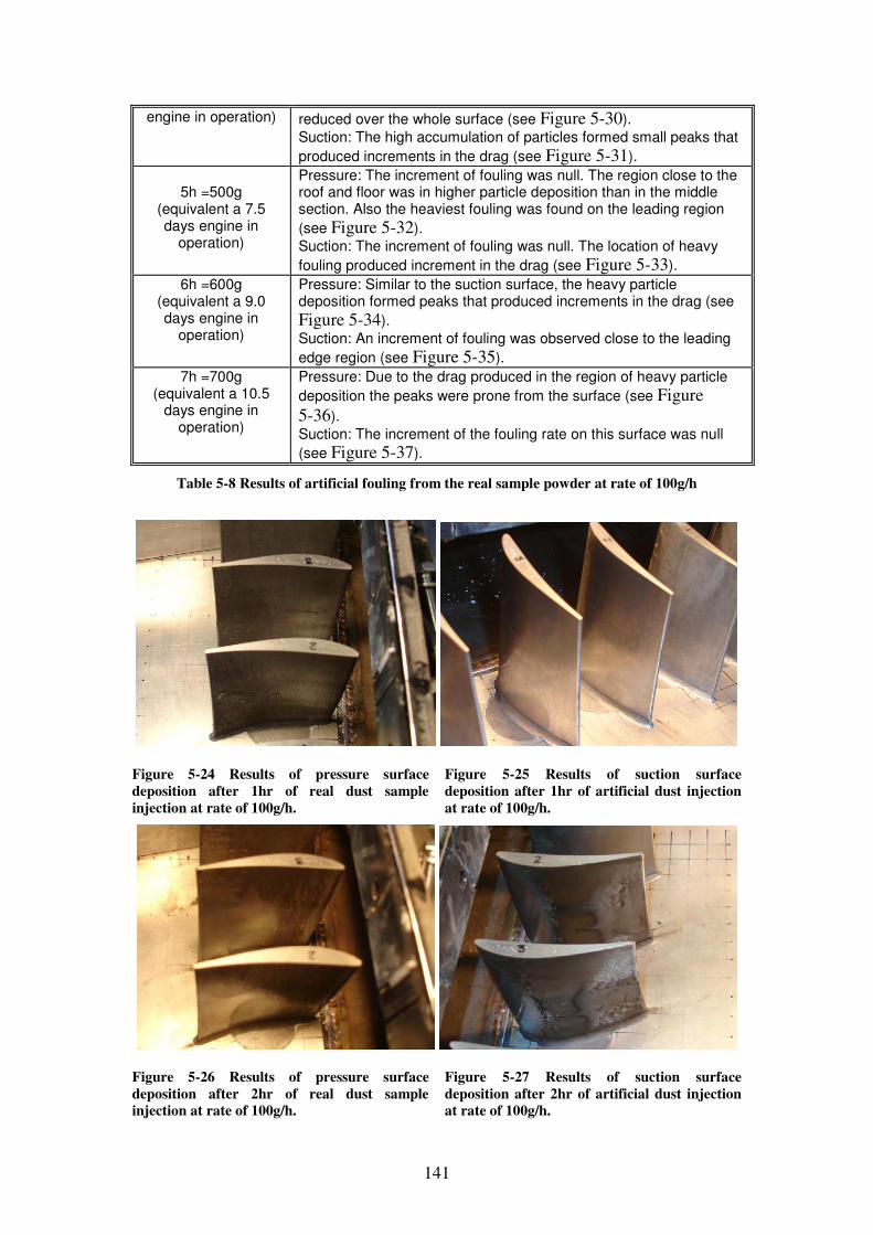
141
engine in operation) reduced over the whole surface (see Figure 5-30).
Suction: The high accumulation of particles formed small peaks that
produced increments in the drag (see Figure 5-31).
5h =500g
(equivalent a 7.5 days engine in
operation)
Pressure: The increment of fouling was null. The region close to the roof and floor was in higher particle deposition than in the middle section. Also the heaviest fouling was found on the leading region
(see Figure 5-32).
Suction: The increment of fouling was null. The location of heavy
fouling produced increment in the drag (see Figure 5-33).
6h =600g (equivalent a 9.0 days engine in
operation)
Pressure: Similar to the suction surface, the heavy particle deposition formed peaks that produced increments in the drag (see
Figure 5-34).
Suction: An increment of fouling was observed close to the leading
edge region (see Figure 5-35).
7h =700g (equivalent a 10.5
days engine in operation)
Pressure: Due to the drag produced in the region of heavy particle
deposition the peaks were prone from the surface (see Figure 5-36).
Suction: The increment of the fouling rate on this surface was null
(see Figure 5-37).
Table 5-8 Results of artificial fouling from the real sample powder at rate of 100g/h
Figure 5-24 Results of pressure surface
deposition after 1hr of real dust sample
injection at rate of 100g/h.
Figure 5-25 Results of suction surface
deposition after 1hr of artificial dust injection
at rate of 100g/h.
Figure 5-26 Results of pressure surface
deposition after 2hr of real dust sample
injection at rate of 100g/h.
Figure 5-27 Results of suction surface
deposition after 2hr of artificial dust injection
at rate of 100g/h.
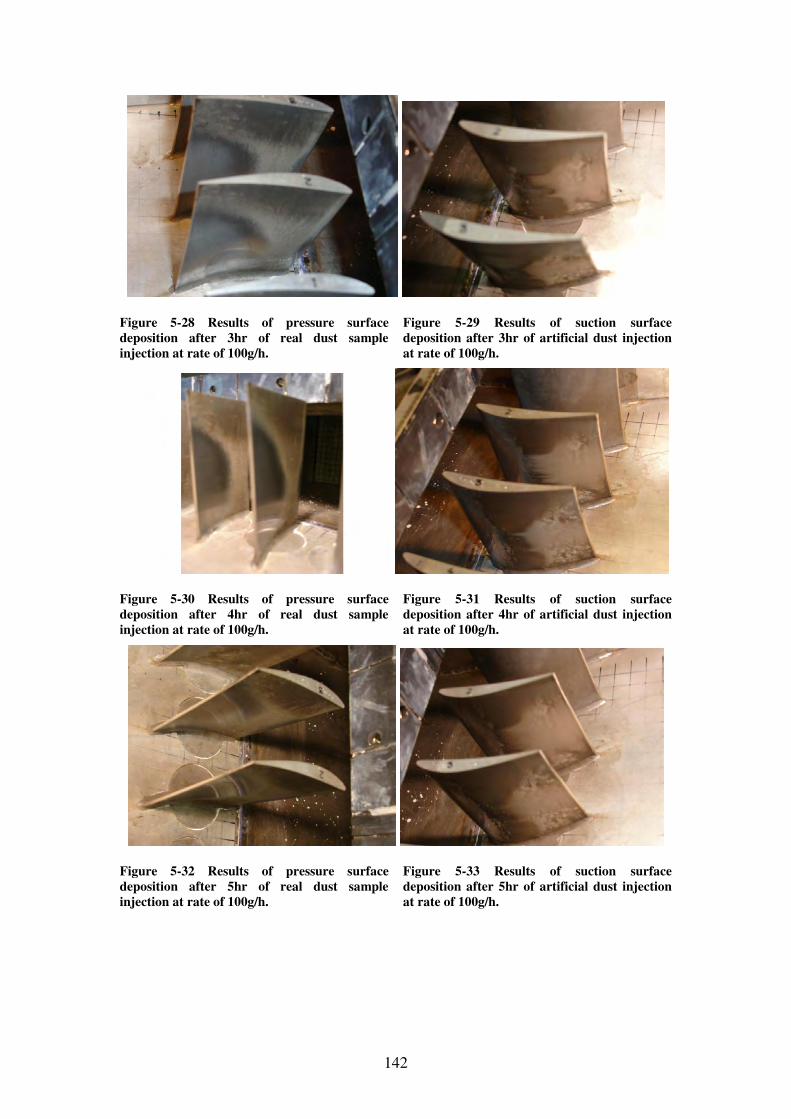
142
Figure 5-28 Results of pressure surface
deposition after 3hr of real dust sample
injection at rate of 100g/h.
Figure 5-29 Results of suction surface
deposition after 3hr of artificial dust injection
at rate of 100g/h.
Figure 5-30 Results of pressure surface
deposition after 4hr of real dust sample
injection at rate of 100g/h.
Figure 5-31 Results of suction surface
deposition after 4hr of artificial dust injection
at rate of 100g/h.
Figure 5-32 Results of pressure surface
deposition after 5hr of real dust sample
injection at rate of 100g/h.
Figure 5-33 Results of suction surface
deposition after 5hr of artificial dust injection
at rate of 100g/h.
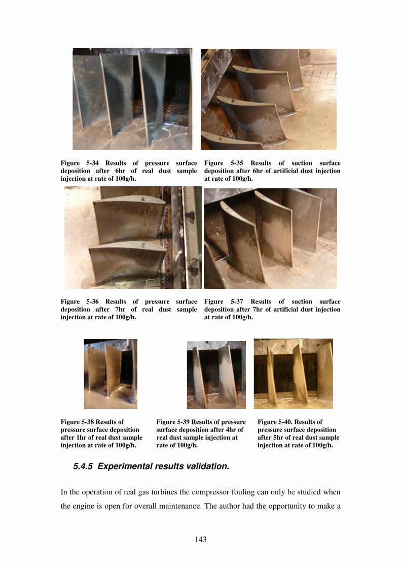
143
Figure 5-34 Results of pressure surface
deposition after 6hr of real dust sample
injection at rate of 100g/h.
Figure 5-35 Results of suction surface
deposition after 6hr of artificial dust injection
at rate of 100g/h.
Figure 5-36 Results of pressure surface
deposition after 7hr of real dust sample
injection at rate of 100g/h.
Figure 5-37 Results of suction surface
deposition after 7hr of artificial dust injection
at rate of 100g/h.
Figure 5-38 Results of
pressure surface deposition
after 1hr of real dust sample
injection at rate of 100g/h.
Figure 5-39 Results of pressure
surface deposition after 4hr of
real dust sample injection at
rate of 100g/h.
Figure 5-40. Results of
pressure surface deposition
after 5hr of real dust sample
injection at rate of 100g/h.
5.4.5 Experimental results validation.
In the operation of real gas turbines the compressor fouling can only be studied when
the engine is open for overall maintenance. The author had the opportunity to make a
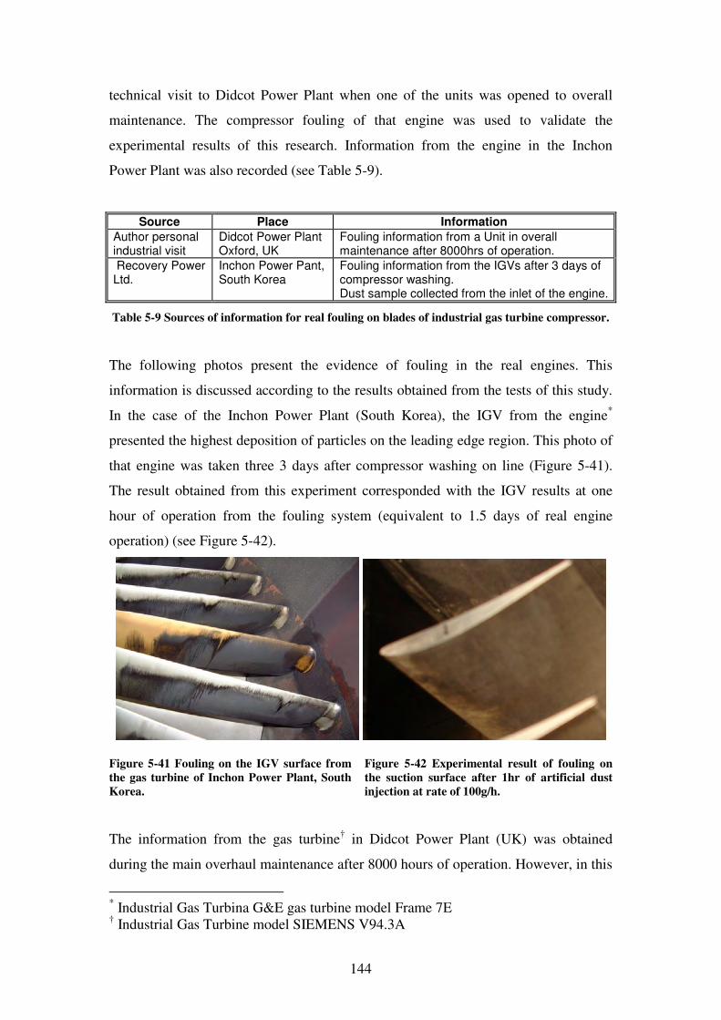
144
technical visit to Didcot Power Plant when one of the units was opened to overall
maintenance. The compressor fouling of that engine was used to validate the
experimental results of this research. Information from the engine in the Inchon
Power Plant was also recorded (see Table 5-9).
Source Place Information
Author personal industrial visit
Didcot Power Plant Oxford, UK
Fouling information from a Unit in overall maintenance after 8000hrs of operation.
Recovery Power Ltd.
Inchon Power Pant, South Korea
Fouling information from the IGVs after 3 days of compressor washing. Dust sample collected from the inlet of the engine.
Table 5-9 Sources of information for real fouling on blades of industrial gas turbine compressor.
The following photos present the evidence of fouling in the real engines. This
information is discussed according to the results obtained from the tests of this study.
In the case of the Inchon Power Plant (South Korea), the IGV from the engine*
presented the highest deposition of particles on the leading edge region. This photo of
that engine was taken three 3 days after compressor washing on line (Figure 5-41).
The result obtained from this experiment corresponded with the IGV results at one
hour of operation from the fouling system (equivalent to 1.5 days of real engine
operation) (see Figure 5-42).
Figure 5-41 Fouling on the IGV surface from
the gas turbine of Inchon Power Plant, South
Korea.
Figure 5-42 Experimental result of fouling on
the suction surface after 1hr of artificial dust
injection at rate of 100g/h.
The information from the gas turbine† in Didcot Power Plant (UK) was obtained
during the main overhaul maintenance after 8000 hours of operation. However, in this
* Industrial Gas Turbina G&E gas turbine model Frame 7E † Industrial Gas Turbine model SIEMENS V94.3A
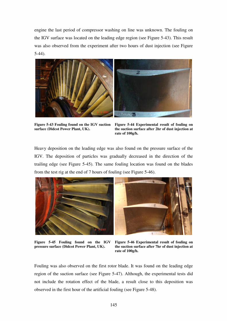
145
engine the last period of compressor washing on line was unknown. The fouling on
the IGV surface was located on the leading edge region (see Figure 5-43). This result
was also observed from the experiment after two hours of dust injection (see Figure
5-44).
Figure 5-43 Fouling found on the IGV suction
surface (Didcot Power Plant, UK).
Figure 5-44 Experimental result of fouling on
the suction surface after 2hr of dust injection at
rate of 100g/h.
Heavy deposition on the leading edge was also found on the pressure surface of the
IGV. The deposition of particles was gradually decreased in the direction of the
trailing edge (see Figure 5-45). The same fouling location was found on the blades
from the test rig at the end of 7 hours of fouling (see Figure 5-46).
Figure 5-45 Fouling found on the IGV
pressure surface (Didcot Power Plant, UK).
Figure 5-46 Experimental result of fouling on
the suction surface after 7hr of dust injection at
rate of 100g/h.
Fouling was also observed on the first rotor blade. It was found on the leading edge
region of the suction surface (see Figure 5-47). Although, the experimental tests did
not include the rotation effect of the blade, a result close to this deposition was
observed in the first hour of the artificial fouling (see Figure 5-48).
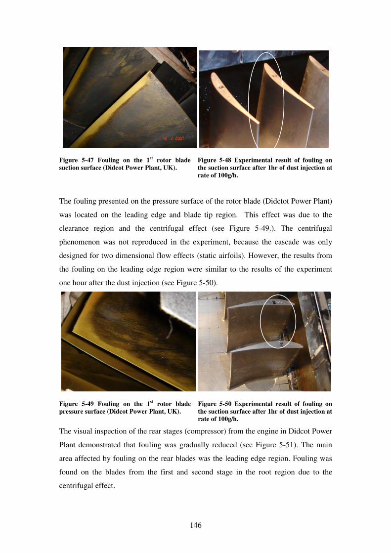
146
Figure 5-47 Fouling on the 1st rotor blade
suction surface (Didcot Power Plant, UK).
Figure 5-48 Experimental result of fouling on
the suction surface after 1hr of dust injection at
rate of 100g/h.
The fouling presented on the pressure surface of the rotor blade (Didctot Power Plant)
was located on the leading edge and blade tip region. This effect was due to the
clearance region and the centrifugal effect (see Figure 5-49.). The centrifugal
phenomenon was not reproduced in the experiment, because the cascade was only
designed for two dimensional flow effects (static airfoils). However, the results from
the fouling on the leading edge region were similar to the results of the experiment
one hour after the dust injection (see Figure 5-50).
Figure 5-49 Fouling on the 1st rotor blade
pressure surface (Didcot Power Plant, UK).
Figure 5-50 Experimental result of fouling on
the suction surface after 1hr of dust injection at
rate of 100g/h.
The visual inspection of the rear stages (compressor) from the engine in Didcot Power
Plant demonstrated that fouling was gradually reduced (see Figure 5-51). The main
area affected by fouling on the rear blades was the leading edge region. Fouling was
found on the blades from the first and second stage in the root region due to the
centrifugal effect.
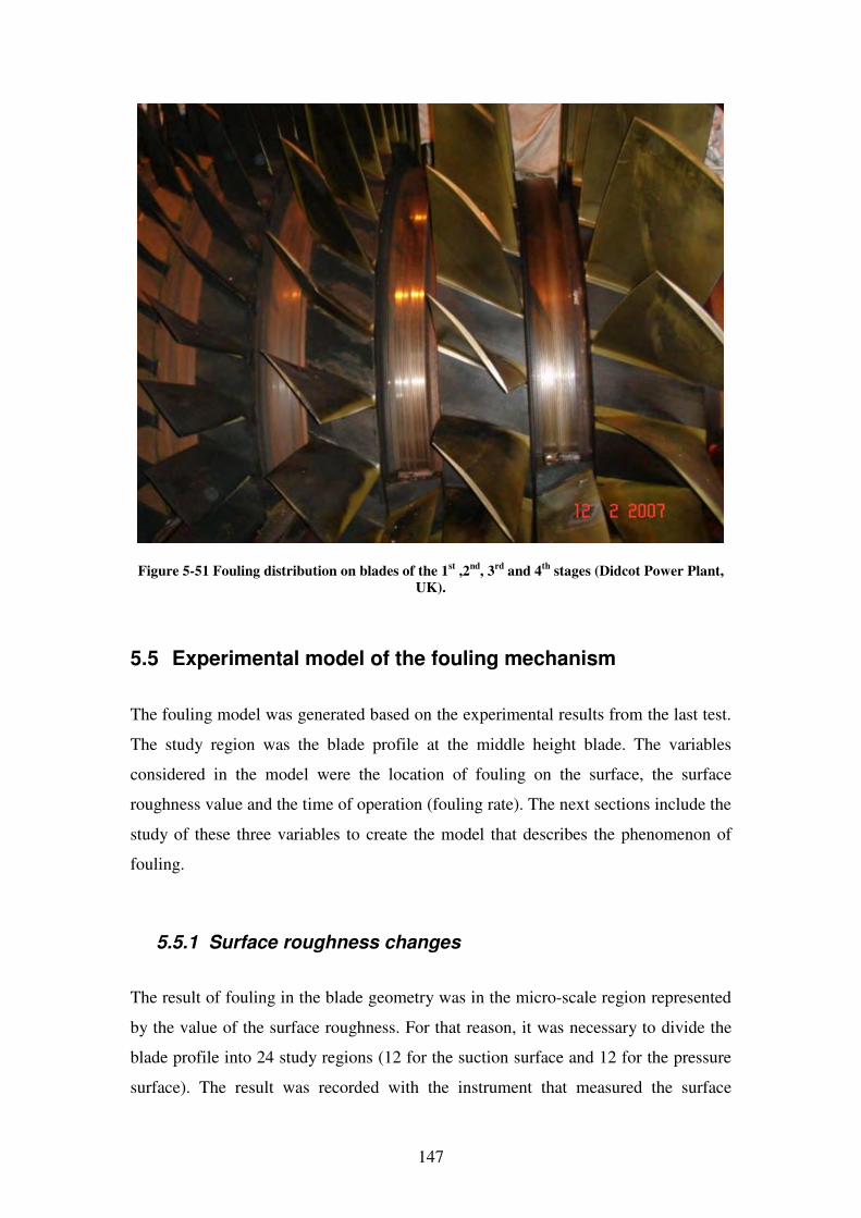
147
Figure 5-51 Fouling distribution on blades of the 1st ,2
nd, 3
rd and 4
th stages (Didcot Power Plant,
UK).
5.5 Experimental model of the fouling mechanism
The fouling model was generated based on the experimental results from the last test.
The study region was the blade profile at the middle height blade. The variables
considered in the model were the location of fouling on the surface, the surface
roughness value and the time of operation (fouling rate). The next sections include the
study of these three variables to create the model that describes the phenomenon of
fouling.
5.5.1 Surface roughness changes
The result of fouling in the blade geometry was in the micro-scale region represented
by the value of the surface roughness. For that reason, it was necessary to divide the
blade profile into 24 study regions (12 for the suction surface and 12 for the pressure
surface). The result was recorded with the instrument that measured the surface
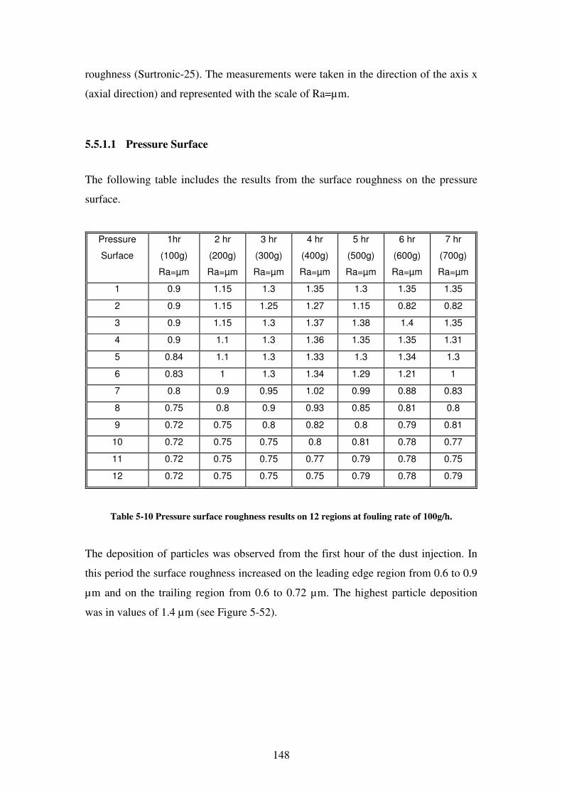
148
roughness (Surtronic-25). The measurements were taken in the direction of the axis x
(axial direction) and represented with the scale of Ra=µm.
5.5.1.1 Pressure Surface
The following table includes the results from the surface roughness on the pressure
surface.
Pressure
Surface
1hr
(100g)
Ra=µm
2 hr
(200g)
Ra=µm
3 hr
(300g)
Ra=µm
4 hr
(400g)
Ra=µm
5 hr
(500g)
Ra=µm
6 hr
(600g)
Ra=µm
7 hr
(700g)
Ra=µm
1 0.9 1.15 1.3 1.35 1.3 1.35 1.35
2 0.9 1.15 1.25 1.27 1.15 0.82 0.82
3 0.9 1.15 1.3 1.37 1.38 1.4 1.35
4 0.9 1.1 1.3 1.36 1.35 1.35 1.31
5 0.84 1.1 1.3 1.33 1.3 1.34 1.3
6 0.83 1 1.3 1.34 1.29 1.21 1
7 0.8 0.9 0.95 1.02 0.99 0.88 0.83
8 0.75 0.8 0.9 0.93 0.85 0.81 0.8
9 0.72 0.75 0.8 0.82 0.8 0.79 0.81
10 0.72 0.75 0.75 0.8 0.81 0.78 0.77
11 0.72 0.75 0.75 0.77 0.79 0.78 0.75
12 0.72 0.75 0.75 0.75 0.79 0.78 0.79
Table 5-10 Pressure surface roughness results on 12 regions at fouling rate of 100g/h.
The deposition of particles was observed from the first hour of the dust injection. In
this period the surface roughness increased on the leading edge region from 0.6 to 0.9
µm and on the trailing region from 0.6 to 0.72 µm. The highest particle deposition
was in values of 1.4 µm (see Figure 5-52).
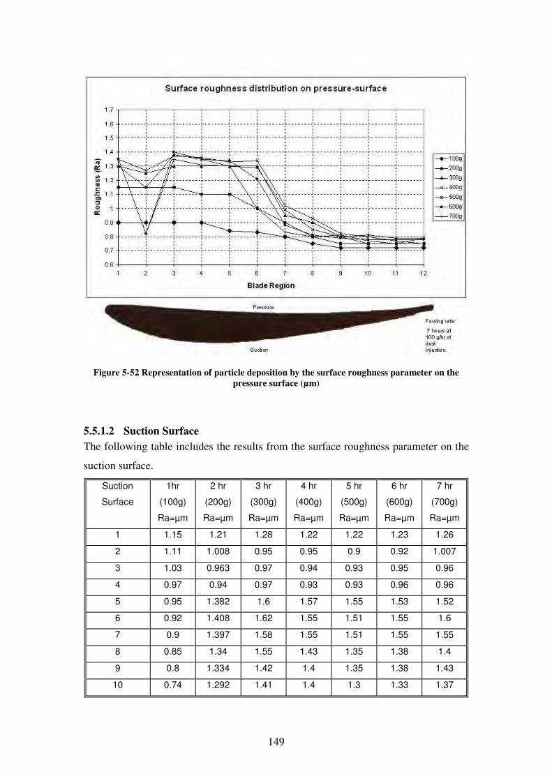
149
Figure 5-52 Representation of particle deposition by the surface roughness parameter on the
pressure surface (µm)
5.5.1.2 Suction Surface
The following table includes the results from the surface roughness parameter on the
suction surface.
Suction
Surface
1hr
(100g)
Ra=µm
2 hr
(200g)
Ra=µm
3 hr
(300g)
Ra=µm
4 hr
(400g)
Ra=µm
5 hr
(500g)
Ra=µm
6 hr
(600g)
Ra=µm
7 hr
(700g)
Ra=µm
1 1.15 1.21 1.28 1.22 1.22 1.23 1.26
2 1.11 1.008 0.95 0.95 0.9 0.92 1.007
3 1.03 0.963 0.97 0.94 0.93 0.95 0.96
4 0.97 0.94 0.97 0.93 0.93 0.96 0.96
5 0.95 1.382 1.6 1.57 1.55 1.53 1.52
6 0.92 1.408 1.62 1.55 1.51 1.55 1.6
7 0.9 1.397 1.58 1.55 1.51 1.55 1.55
8 0.85 1.34 1.55 1.43 1.35 1.38 1.4
9 0.8 1.334 1.42 1.4 1.35 1.38 1.43
10 0.74 1.292 1.41 1.4 1.3 1.33 1.37
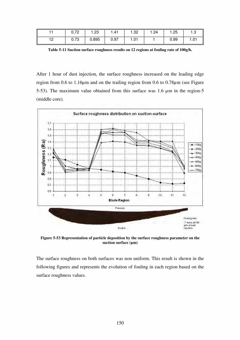
150
11 0.72 1.23 1.41 1.32 1.24 1.25 1.3
12 0.73 0.895 0.97 1.01 1 0.99 1.01
Table 5-11 Suction surface roughness results on 12 regions at fouling rate of 100g/h.
After 1 hour of dust injection, the surface roughness increased on the leading edge
region from 0.6 to 1.16µm and on the trailing region from 0.6 to 0.78µm (see Figure
5-53). The maximum value obtained from this surface was 1.6 µm in the region-5
(middle core).
Figure 5-53 Representation of particle deposition by the surface roughness parameter on the
suction surface (µm)
The surface roughness on both surfaces was non uniform. This result is shown in the
following figures and represents the evolution of fouling in each region based on the
surface roughness values.
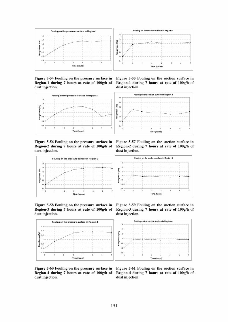
151
Fouling on the pressure-surface in Region-1
0.4
0.6
0.8
1
1.2
1.4
1.6
0 1 2 3 4 5 6 7
Time (hours)
Ro
ug
hn
ess
(R
a)
Fouling on the suction-surface in Region-1
0.4
0.6
0.8
1
1.2
1.4
1.6
0 1 2 3 4 5 6 7
Time (hours)
Ro
ug
hn
es
s (
Ra
)
Figure 5-54 Fouling on the pressure surface in
Region-1 during 7 hours at rate of 100g/h of
dust injection.
Figure 5-55 Fouling on the suction surface in
Region-1 during 7 hours at rate of 100g/h of
dust injection.
Fouling on the pressure-surface in Region-2
0.4
0.6
0.8
1
1.2
1.4
1.6
0 1 2 3 4 5 6 7
Time (hours)
Ro
ug
hn
ess
(R
a)
Fouling on the suction surface in Region-2
0.4
0.6
0.8
1
1.2
1.4
1.6
0 1 2 3 4 5 6 7
Time (hours)
Ro
ug
hn
es
s (R
a)
Figure 5-56 Fouling on the pressure surface in
Region-2 during 7 hours at rate of 100g/h of
dust injection.
Figure 5-57 Fouling on the suction surface in
Region-2 during 7 hours at rate of 100g/h of
dust injection.
Fouling on the pressure-surface in Region-3
0.4
0.6
0.8
1
1.2
1.4
1.6
0 1 2 3 4 5 6 7
Time (hours)
Ro
ug
hn
ess (
Ra
)
Fouling on the suction surface in Region-3
0.4
0.6
0.8
1
1.2
1.4
1.6
0 1 2 3 4 5 6 7
Time (hours)
Ro
ug
hn
ess (R
a)
Figure 5-58 Fouling on the pressure surface in
Region-3 during 7 hours at rate of 100g/h of
dust injection.
Figure 5-59 Fouling on the suction surface in
Region-3 during 7 hours at rate of 100g/h of
dust injection.
Fouling on the pressure-surface in Region-4
0.4
0.6
0.8
1
1.2
1.4
1.6
0 1 2 3 4 5 6 7
Time (hours)
Ro
ug
hn
es
s (
Ra)
Fouling on the suction surface in Region-4
0.4
0.6
0.8
1
1.2
1.4
1.6
0 1 2 3 4 5 6 7
Time (hours)
Ro
ug
hn
ess
(R
a)
Figure 5-60 Fouling on the pressure surface in
Region-4 during 7 hours at rate of 100g/h of
dust injection.
Figure 5-61 Fouling on the suction surface in
Region-4 during 7 hours at rate of 100g/h of
dust injection.
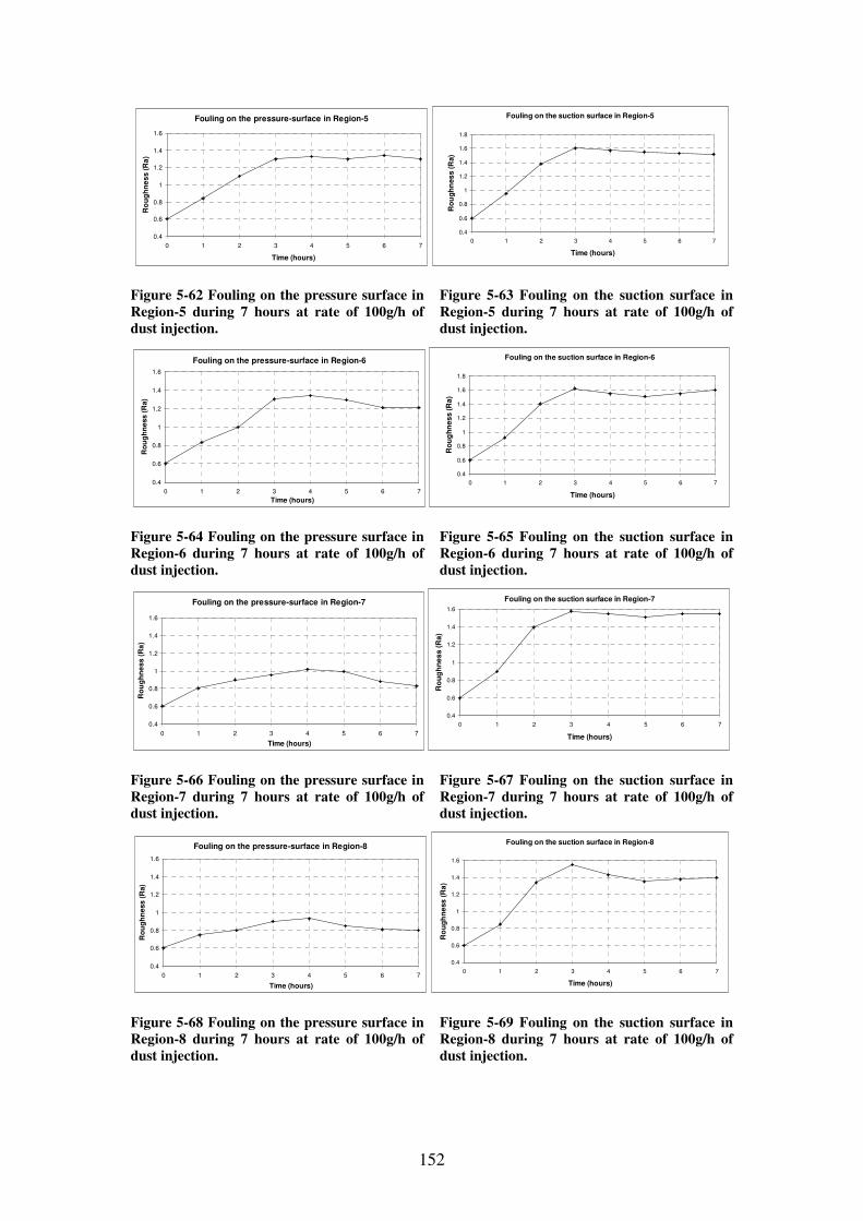
152
Fouling on the pressure-surface in Region-5
0.4
0.6
0.8
1
1.2
1.4
1.6
0 1 2 3 4 5 6 7
Time (hours)
Ro
ug
hn
es
s (
Ra
)
Fouling on the suction surface in Region-5
0.4
0.6
0.8
1
1.2
1.4
1.6
1.8
0 1 2 3 4 5 6 7
Time (hours)
Ro
ug
hn
es
s (R
a)
Figure 5-62 Fouling on the pressure surface in
Region-5 during 7 hours at rate of 100g/h of
dust injection.
Figure 5-63 Fouling on the suction surface in
Region-5 during 7 hours at rate of 100g/h of
dust injection.
Fouling on the pressure-surface in Region-6
0.4
0.6
0.8
1
1.2
1.4
1.6
0 1 2 3 4 5 6 7
Time (hours)
Ro
ug
hn
ess
(R
a)
Fouling on the suction surface in Region-6
0.4
0.6
0.8
1
1.2
1.4
1.6
1.8
0 1 2 3 4 5 6 7
Time (hours)
Ro
ug
hn
es
s (
Ra
)
Figure 5-64 Fouling on the pressure surface in
Region-6 during 7 hours at rate of 100g/h of
dust injection.
Figure 5-65 Fouling on the suction surface in
Region-6 during 7 hours at rate of 100g/h of
dust injection.
Fouling on the pressure-surface in Region-7
0.4
0.6
0.8
1
1.2
1.4
1.6
0 1 2 3 4 5 6 7
Time (hours)
Ro
ug
hn
ess
(R
a)
Fouling on the suction surface in Region-7
0.4
0.6
0.8
1
1.2
1.4
1.6
0 1 2 3 4 5 6 7
Time (hours)
Ro
ug
hn
es
s (
Ra
)
Figure 5-66 Fouling on the pressure surface in
Region-7 during 7 hours at rate of 100g/h of
dust injection.
Figure 5-67 Fouling on the suction surface in
Region-7 during 7 hours at rate of 100g/h of
dust injection.
Fouling on the pressure-surface in Region-8
0.4
0.6
0.8
1
1.2
1.4
1.6
0 1 2 3 4 5 6 7
Time (hours)
Ro
ug
hn
ess
(R
a)
Fouling on the suction surface in Region-8
0.4
0.6
0.8
1
1.2
1.4
1.6
0 1 2 3 4 5 6 7
Time (hours)
Ro
ug
hn
ess
(R
a)
Figure 5-68 Fouling on the pressure surface in
Region-8 during 7 hours at rate of 100g/h of
dust injection.
Figure 5-69 Fouling on the suction surface in
Region-8 during 7 hours at rate of 100g/h of
dust injection.
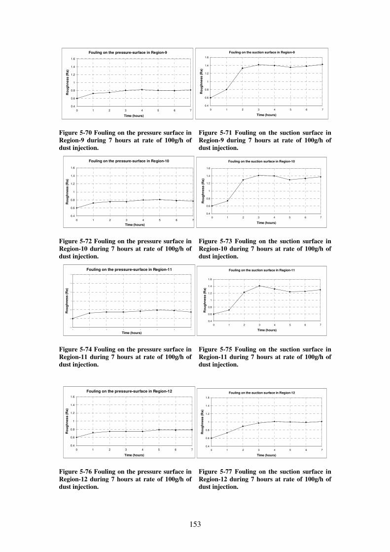
153
Fouling on the pressure-surface in Region-9
0.4
0.6
0.8
1
1.2
1.4
1.6
0 1 2 3 4 5 6 7
Time (hours)
Ro
ug
hn
ess
(R
a)
Fouling on the suction surface in Region-9
0.4
0.6
0.8
1
1.2
1.4
1.6
0 1 2 3 4 5 6 7
Time (hours)
Ro
ug
hn
ess (R
a)
Figure 5-70 Fouling on the pressure surface in
Region-9 during 7 hours at rate of 100g/h of
dust injection.
Figure 5-71 Fouling on the suction surface in
Region-9 during 7 hours at rate of 100g/h of
dust injection.
Fouling on the pressure-surface in Region-10
0.4
0.6
0.8
1
1.2
1.4
1.6
0 1 2 3 4 5 6 7
Time (hours)
Ro
ug
hn
ess
(R
a)
Fouling on the suction surface in Region-10
0.4
0.6
0.8
1
1.2
1.4
1.6
0 1 2 3 4 5 6 7
Time (hours)
Ro
ug
hn
es
s (
Ra
)
Figure 5-72 Fouling on the pressure surface in
Region-10 during 7 hours at rate of 100g/h of
dust injection.
Figure 5-73 Fouling on the suction surface in
Region-10 during 7 hours at rate of 100g/h of
dust injection.
Fouling on the pressure-surface in Region-11
0.4
0.6
0.8
1
1.2
1.4
1.6
0 1 2 3 4 5 6 7
Time (hours)
Ro
ug
hn
ess (
Ra)
Fouling on the suction surface in Region-11
0.4
0.6
0.8
1
1.2
1.4
1.6
0 1 2 3 4 5 6 7
Time (hours)
Ro
ug
hn
es
s (R
a)
Figure 5-74 Fouling on the pressure surface in
Region-11 during 7 hours at rate of 100g/h of
dust injection.
Figure 5-75 Fouling on the suction surface in
Region-11 during 7 hours at rate of 100g/h of
dust injection.
Fouling on the pressure-surface in Region-12
0.4
0.6
0.8
1
1.2
1.4
1.6
0 1 2 3 4 5 6 7
Time (hours)
Ro
ug
hn
es
s (
Ra)
Fouling on the suction surface in Region-12
0.4
0.6
0.8
1
1.2
1.4
1.6
0 1 2 3 4 5 6 7
Time (hours)
Ro
ug
hn
ess
(R
a)
Figure 5-76 Fouling on the pressure surface in
Region-12 during 7 hours at rate of 100g/h of
dust injection.
Figure 5-77 Fouling on the suction surface in
Region-12 during 7 hours at rate of 100g/h of
dust injection.
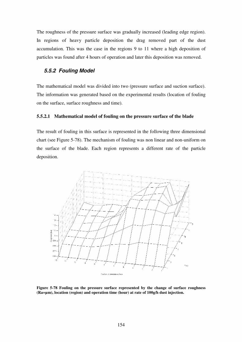
154
The roughness of the pressure surface was gradually increased (leading edge region).
In regions of heavy particle deposition the drag removed part of the dust
accumulation. This was the case in the regions 9 to 11 where a high deposition of
particles was found after 4 hours of operation and later this deposition was removed.
5.5.2 Fouling Model
The mathematical model was divided into two (pressure surface and suction surface).
The information was generated based on the experimental results (location of fouling
on the surface, surface roughness and time).
5.5.2.1 Mathematical model of fouling on the pressure surface of the blade
The result of fouling in this surface is represented in the following three dimensional
chart (see Figure 5-78). The mechanism of fouling was non linear and non-uniform on
the surface of the blade. Each region represents a different rate of the particle
deposition.
Figure 5-78 Fouling on the pressure surface represented by the change of surface roughness
(Ra=µm), location (region) and operation time (hour) at rate of 100g/h dust injection.
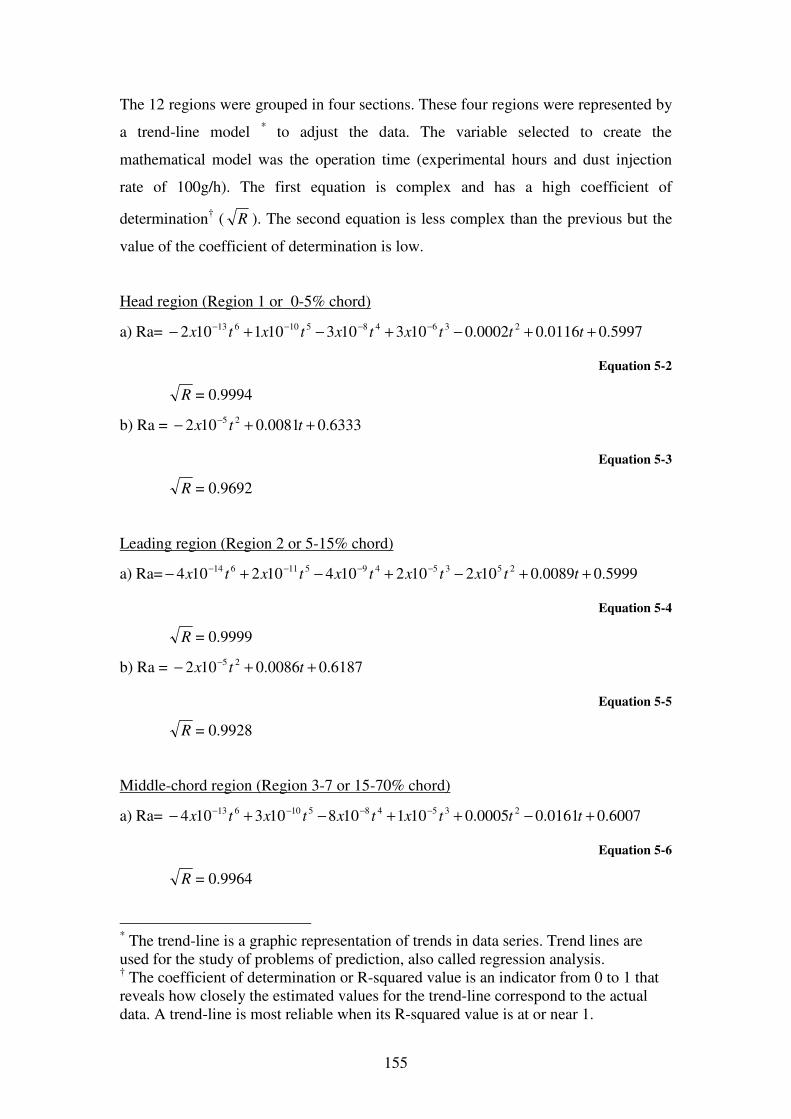
155
The 12 regions were grouped in four sections. These four regions were represented by
a trend-line model * to adjust the data. The variable selected to create the
mathematical model was the operation time (experimental hours and dust injection
rate of 100g/h). The first equation is complex and has a high coefficient of
determination† ( R ). The second equation is less complex than the previous but the
value of the coefficient of determination is low.
Head region (Region 1 or 0-5% chord)
a) Ra= 5997.00116.00002.0103103101102 23648510613 ++−+−+− −−−−tttxtxtxtx
Equation 5-2
R = 0.9994
b) Ra = 6333.00081.0102 25 ++− −ttx
Equation 5-3
R = 0.9692
Leading region (Region 2 or 5-15% chord)
a) Ra= 5999.00089.0102102104102104 253549511614 ++−+−+− −−−−ttxtxtxtxtx
Equation 5-4
R = 0.9999
b) Ra = 6187.00086.0102 25 ++− −ttx
Equation 5-5
R = 0.9928
Middle-chord region (Region 3-7 or 15-70% chord)
a) Ra= 6007.00161.00005.0101108103104 23548510613 +−++−+− −−−−tttxtxtxtx
Equation 5-6
R = 0.9964
* The trend-line is a graphic representation of trends in data series. Trend lines are used for the study of problems of prediction, also called regression analysis. † The coefficient of determination or R-squared value is an indicator from 0 to 1 that reveals how closely the estimated values for the trend-line correspond to the actual data. A trend-line is most reliable when its R-squared value is at or near 1.
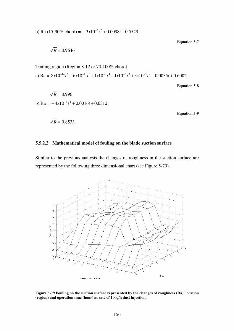
156
b) Ra (15-90% chord) = 5529.00098.0103 25 ++− −ttx
Equation 5-7
R = 0.9646
Trailing region (Region 8-12 or 70-100% chord)
a) Ra = 6002.00035.0103101101106108 253648511614 +−+−+− −−−−−ttxtxtxtxtx
Equation 5-8
R = 0.996
b) Ra = 6312.00016.0104 26 ++− −ttx
Equation 5-9
R = 0.8533
5.5.2.2 Mathematical model of fouling on the blade suction surface
Similar to the previous analysis the changes of roughness in the suction surface are
represented by the following three dimensional chart (see Figure 5-79).
Figure 5-79 Fouling on the suction surface represented by the changes of roughness (Ra), location
(region) and operation time (hour) at rate of 100g/h dust injection.
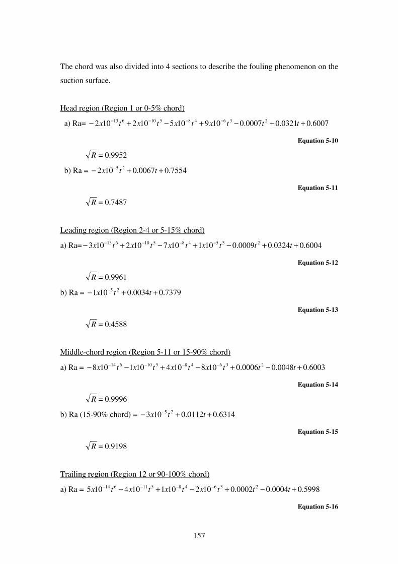
157
The chord was also divided into 4 sections to describe the fouling phenomenon on the
suction surface.
Head region (Region 1 or 0-5% chord)
a) Ra= 6007.00321.00007.0109105102102 23648510613 ++−+−+− −−−−tttxtxtxtx
Equation 5-10
R = 0.9952
b) Ra = 7554.00067.0102 25 ++− −ttx
Equation 5-11
R = 0.7487
Leading region (Region 2-4 or 5-15% chord)
a) Ra= 6004.00324.00009.0101107102103 23548510613 ++−+−+− −−−−tttxtxtxtx
Equation 5-12
R = 0.9961
b) Ra = 7379.00034.0101 25 ++− −ttx
Equation 5-13
R = 0.4588
Middle-chord region (Region 5-11 or 15-90% chord)
a) Ra = 6003.00048.00006.0108104101108 23648510614 +−+−+−− −−−−tttxtxtxtx
Equation 5-14
R = 0.9996
b) Ra (15-90% chord) = 6314.00112.0103 25 ++− −ttx
Equation 5-15
R = 0.9198
Trailing region (Region 12 or 90-100% chord)
a) Ra = 5998.00004.00002.0102101104105 23648511614 +−+−+− −−−−tttxtxtxtx
Equation 5-16
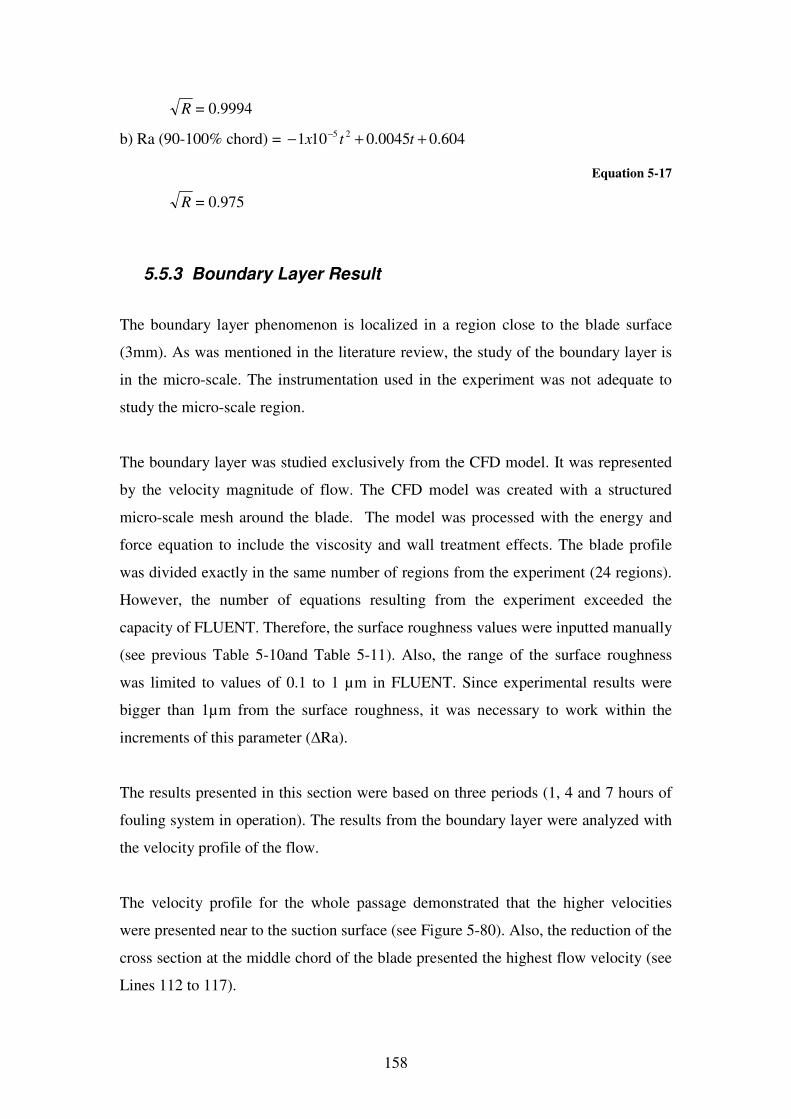
158
R = 0.9994
b) Ra (90-100% chord) = 604.00045.0101 25 ++− −ttx
Equation 5-17
R = 0.975
5.5.3 Boundary Layer Result
The boundary layer phenomenon is localized in a region close to the blade surface
(3mm). As was mentioned in the literature review, the study of the boundary layer is
in the micro-scale. The instrumentation used in the experiment was not adequate to
study the micro-scale region.
The boundary layer was studied exclusively from the CFD model. It was represented
by the velocity magnitude of flow. The CFD model was created with a structured
micro-scale mesh around the blade. The model was processed with the energy and
force equation to include the viscosity and wall treatment effects. The blade profile
was divided exactly in the same number of regions from the experiment (24 regions).
However, the number of equations resulting from the experiment exceeded the
capacity of FLUENT. Therefore, the surface roughness values were inputted manually
(see previous Table 5-10and Table 5-11). Also, the range of the surface roughness
was limited to values of 0.1 to 1 µm in FLUENT. Since experimental results were
bigger than 1µm from the surface roughness, it was necessary to work within the
increments of this parameter (∆Ra).
The results presented in this section were based on three periods (1, 4 and 7 hours of
fouling system in operation). The results from the boundary layer were analyzed with
the velocity profile of the flow.
The velocity profile for the whole passage demonstrated that the higher velocities
were presented near to the suction surface (see Figure 5-80). Also, the reduction of the
cross section at the middle chord of the blade presented the highest flow velocity (see
Lines 112 to 117).
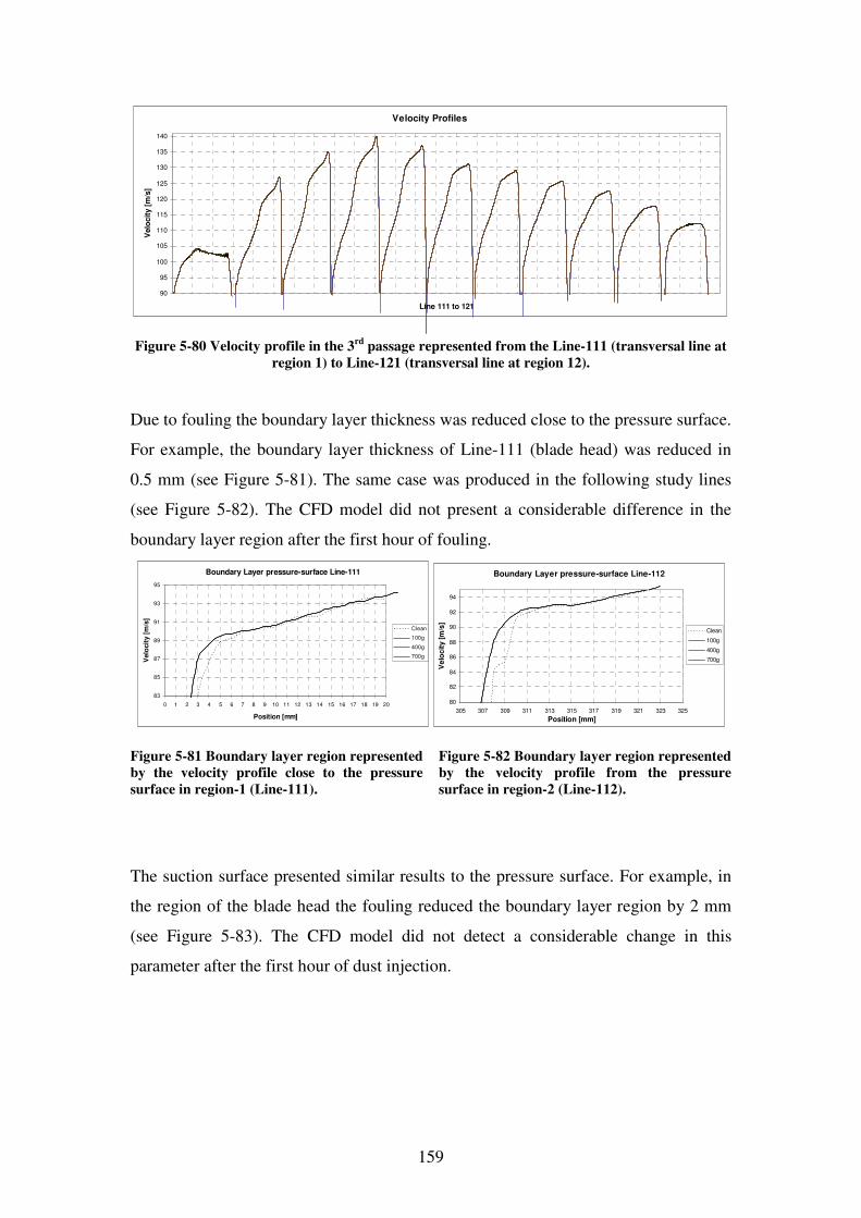
159
Velocity Profiles
90
95
100
105
110
115
120
125
130
135
140
Line 111 to 121
Velo
cit
y [
m/s
]
Figure 5-80 Velocity profile in the 3rd
passage represented from the Line-111 (transversal line at
region 1) to Line-121 (transversal line at region 12).
Due to fouling the boundary layer thickness was reduced close to the pressure surface.
For example, the boundary layer thickness of Line-111 (blade head) was reduced in
0.5 mm (see Figure 5-81). The same case was produced in the following study lines
(see Figure 5-82). The CFD model did not present a considerable difference in the
boundary layer region after the first hour of fouling.
Boundary Layer pressure-surface Line-111
83
85
87
89
91
93
95
0 1 2 3 4 5 6 7 8 9 10 11 12 13 14 15 16 17 18 19 20
Position [mm]
Velo
cit
y [
m/s
]
Clean
100g
400g
700g
Boundary Layer pressure-surface Line-112
80
82
84
86
88
90
92
94
305 307 309 311 313 315 317 319 321 323 325
Position [mm]
Ve
loc
ity
[m
/s]
Clean
100g
400g
700g
Figure 5-81 Boundary layer region represented
by the velocity profile close to the pressure
surface in region-1 (Line-111).
Figure 5-82 Boundary layer region represented
by the velocity profile from the pressure
surface in region-2 (Line-112).
The suction surface presented similar results to the pressure surface. For example, in
the region of the blade head the fouling reduced the boundary layer region by 2 mm
(see Figure 5-83). The CFD model did not detect a considerable change in this
parameter after the first hour of dust injection.
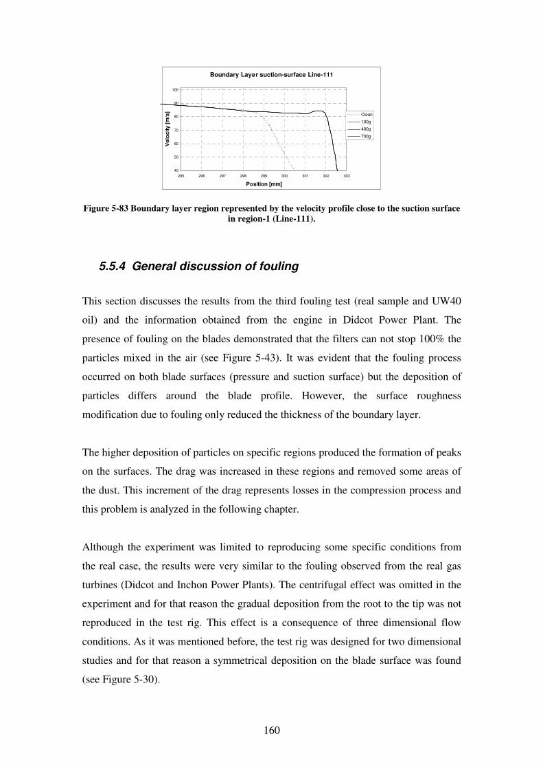
160
Boundary Layer suction-surface Line-111
40
50
60
70
80
90
100
295 296 297 298 299 300 301 302 303
Position [mm]
Ve
loc
ity
[m
/s]
Clean
100g
400g
700g
Figure 5-83 Boundary layer region represented by the velocity profile close to the suction surface
in region-1 (Line-111).
5.5.4 General discussion of fouling
This section discusses the results from the third fouling test (real sample and UW40
oil) and the information obtained from the engine in Didcot Power Plant. The
presence of fouling on the blades demonstrated that the filters can not stop 100% the
particles mixed in the air (see Figure 5-43). It was evident that the fouling process
occurred on both blade surfaces (pressure and suction surface) but the deposition of
particles differs around the blade profile. However, the surface roughness
modification due to fouling only reduced the thickness of the boundary layer.
The higher deposition of particles on specific regions produced the formation of peaks
on the surfaces. The drag was increased in these regions and removed some areas of
the dust. This increment of the drag represents losses in the compression process and
this problem is analyzed in the following chapter.
Although the experiment was limited to reproducing some specific conditions from
the real case, the results were very similar to the fouling observed from the real gas
turbines (Didcot and Inchon Power Plants). The centrifugal effect was omitted in the
experiment and for that reason the gradual deposition from the root to the tip was not
reproduced in the test rig. This effect is a consequence of three dimensional flow
conditions. As it was mentioned before, the test rig was designed for two dimensional
studies and for that reason a symmetrical deposition on the blade surface was found
(see Figure 5-30).

161
The non-uniform fouling on the surfaces demonstrated the necessity to divide the
blade profile into regions. The complex phenomenon was studied in twelve regions of
each surface. However, it was possible to group the results in sections. These results
demonstrated the importance of the fouling problem to affect the original blade
profile. For that reason, the new blades delivered by the OEM were with a low surface
roughness value (0.6 µm) in order to guarantee low losses due to the drag.
162
6 TECHNO-ECONOMIC STUDY OF COMPRESSOR FOULING AND WASHING ON LINE
6.1 Introduction
The preliminary mathematical model of the fouling mechanism was presented in the
previous chapter. This was created based on the experimental particle deposition. The
parameters that were chosen to study this phenomenon were: the blade region of
particles deposition, the modification of the surface roughness and the time of
operation. The results demonstrated that the blade profile played an important role for
the mechanism of fouling. This Chapter studies the application of the fouling model in
a real study case. The first section of this chapter is focused to study the fouling effect
on the blade aerodynamics. The second section analyzes the fouling effect in an
industrial gas turbine. The third section presents a techno economic study based on
the power produced by the engine in order to evaluate the effectiveness of compressor
washing on line.
6.2 Aerodynamics of the blade affected by the fouling mechanism
The results from the experiment and CFD model were studied in this section to
calculate the blade aerodynamics. The static pressure distribution, skin coefficient
distribution and drag force information were calculated from the two dimensional
CFD model.
6.2.1 Static Pressure
The static-pressure distribution in the blade was affected by the increment of the
surface roughness. On the pressure surface this parameter did not change (see Figure
6-1). However, on the suction surface was observed that the static pressure increased
(see Figure 6-2). The region at the middle chord on this surface presented the
maximum static pressure value that coincides with the highest particles deposition
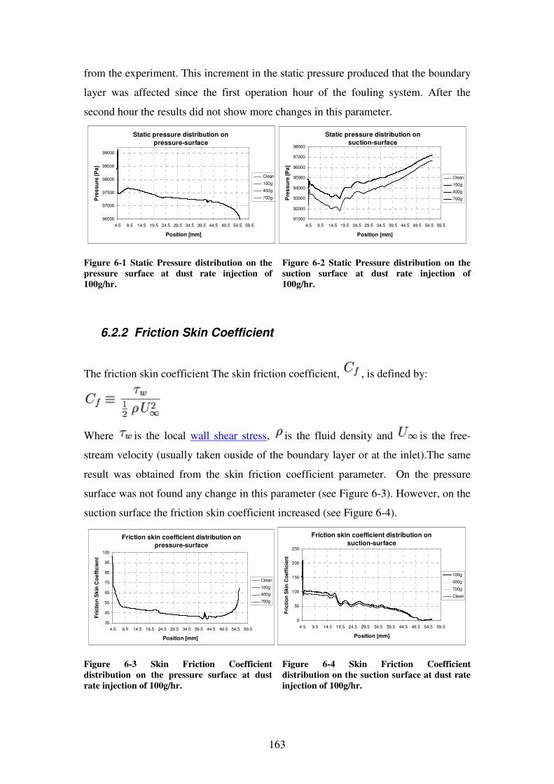
163
from the experiment. This increment in the static pressure produced that the boundary
layer was affected since the first operation hour of the fouling system. After the
second hour the results did not show more changes in this parameter.
Static pressure distribution on
pressure-surface
96500
97000
97500
98000
98500
99000
4.5 9.5 14.5 19.5 24.5 29.5 34.5 39.5 44.5 49.5 54.5 59.5
Position [mm]
Pre
ssu
re [
Pa
]
Clean
100g
400g
700g
Static pressure distribution on
suction-surface
91000
92000
93000
94000
95000
96000
97000
98000
4.5 9.5 14.5 19.5 24.5 29.5 34.5 39.5 44.5 49.5 54.5 59.5
Position [mm]
Pre
ssu
re [P
a]
Clean
100g
400g
700g
Figure 6-1 Static Pressure distribution on the
pressure surface at dust rate injection of
100g/hr.
Figure 6-2 Static Pressure distribution on the
suction surface at dust rate injection of
100g/hr.
6.2.2 Friction Skin Coefficient
The friction skin coefficient The skin friction coefficient, , is defined by:
Where is the local wall shear stress, is the fluid density and is the free-
stream velocity (usually taken ouside of the boundary layer or at the inlet).The same
result was obtained from the skin friction coefficient parameter. On the pressure
surface was not found any change in this parameter (see Figure 6-3). However, on the
suction surface the friction skin coefficient increased (see Figure 6-4).
Friction skin coefficient distribution on
pressure-surface
35
45
55
65
75
85
95
105
4.5 9.5 14.5 19.5 24.5 29.5 34.5 39.5 44.5 49.5 54.5 59.5
Position [mm]
Fri
cti
on
Sk
in C
oe
ffic
ien
t
Clean
100g
400g
700g
Friction skin coefficient distribution on
suction-surface
0
50
100
150
200
250
4.5 9.5 14.5 19.5 24.5 29.5 34.5 39.5 44.5 49.5 54.5 59.5
Position [mm]
Fri
cti
on
Skin
Co
eff
icie
nt
100g
400g
700g
Clean
Figure 6-3 Skin Friction Coefficient
distribution on the pressure surface at dust
rate injection of 100g/hr.
Figure 6-4 Skin Friction Coefficient
distribution on the suction surface at dust rate
injection of 100g/hr.
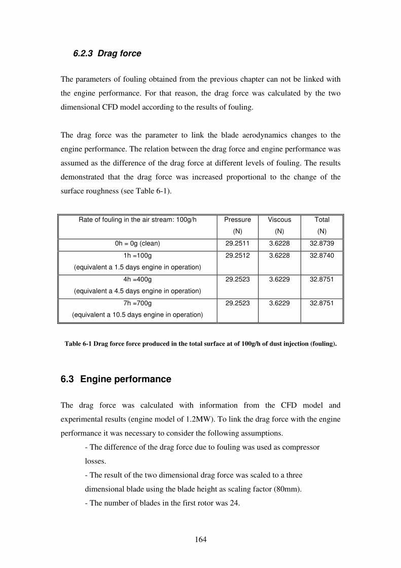
164
6.2.3 Drag force
The parameters of fouling obtained from the previous chapter can not be linked with
the engine performance. For that reason, the drag force was calculated by the two
dimensional CFD model according to the results of fouling.
The drag force was the parameter to link the blade aerodynamics changes to the
engine performance. The relation between the drag force and engine performance was
assumed as the difference of the drag force at different levels of fouling. The results
demonstrated that the drag force was increased proportional to the change of the
surface roughness (see Table 6-1).
Rate of fouling in the air stream: 100g/h Pressure
(N)
Viscous
(N)
Total
(N)
0h = 0g (clean) 29.2511 3.6228 32.8739
1h =100g
(equivalent a 1.5 days engine in operation)
29.2512 3.6228 32.8740
4h =400g
(equivalent a 4.5 days engine in operation)
29.2523 3.6229 32.8751
7h =700g
(equivalent a 10.5 days engine in operation)
29.2523 3.6229 32.8751
Table 6-1 Drag force force produced in the total surface at of 100g/h of dust injection (fouling).
6.3 Engine performance
The drag force was calculated with information from the CFD model and
experimental results (engine model of 1.2MW). To link the drag force with the engine
performance it was necessary to consider the following assumptions.
- The difference of the drag force due to fouling was used as compressor
losses.
- The result of the two dimensional drag force was scaled to a three
dimensional blade using the blade height as scaling factor (80mm).
- The number of blades in the first rotor was 24.
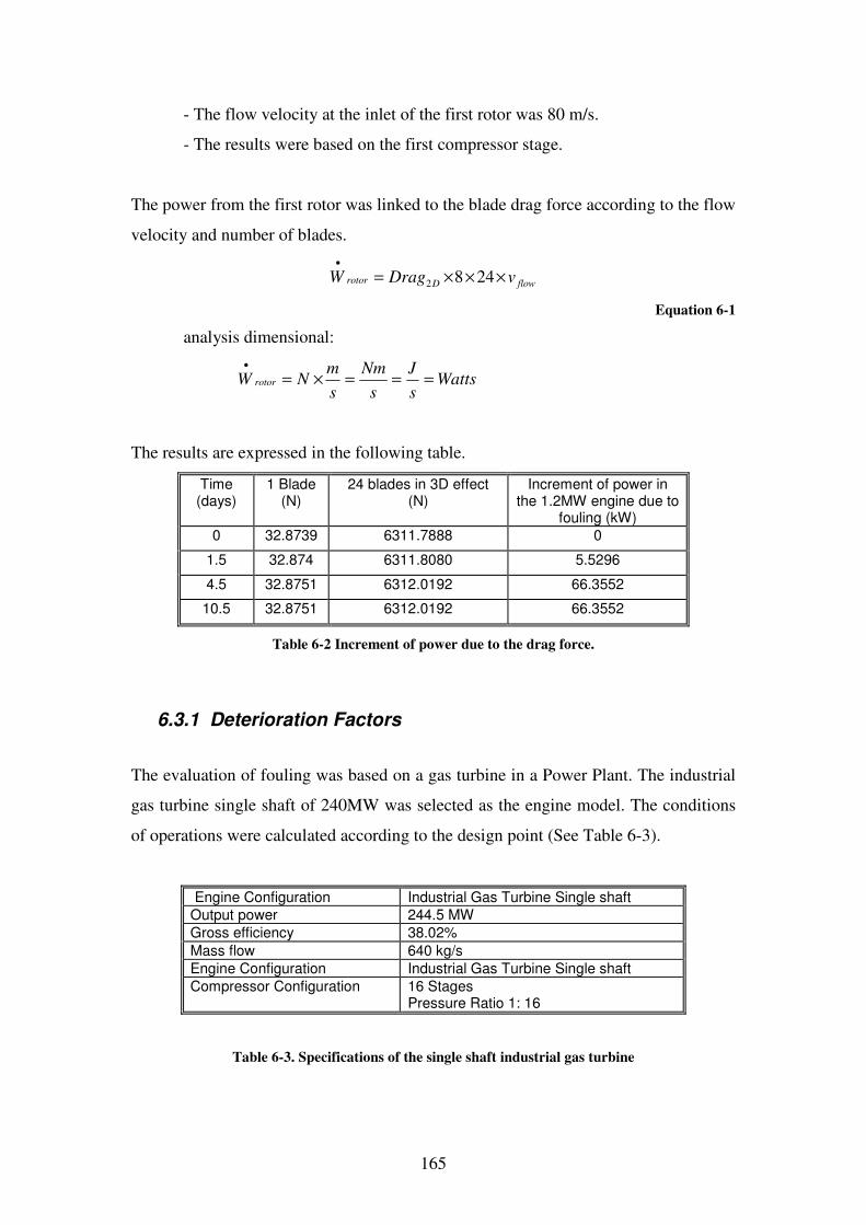
165
- The flow velocity at the inlet of the first rotor was 80 m/s.
- The results were based on the first compressor stage.
The power from the first rotor was linked to the blade drag force according to the flow
velocity and number of blades.
flowDrotor vDragW ×××=•
2482
Equation 6-1
analysis dimensional:
Wattss
J
s
Nm
s
mNW rotor ===×=
•
The results are expressed in the following table.
Time (days)
1 Blade (N)
24 blades in 3D effect (N)
Increment of power in the 1.2MW engine due to
fouling (kW)
0 32.8739 6311.7888 0
1.5 32.874 6311.8080 5.5296
4.5 32.8751 6312.0192 66.3552
10.5 32.8751 6312.0192 66.3552
Table 6-2 Increment of power due to the drag force.
6.3.1 Deterioration Factors
The evaluation of fouling was based on a gas turbine in a Power Plant. The industrial
gas turbine single shaft of 240MW was selected as the engine model. The conditions
of operations were calculated according to the design point (See Table 6-3).
Engine Configuration Industrial Gas Turbine Single shaft
Output power 244.5 MW
Gross efficiency 38.02%
Mass flow 640 kg/s
Engine Configuration Industrial Gas Turbine Single shaft
Compressor Configuration 16 Stages Pressure Ratio 1: 16
Table 6-3. Specifications of the single shaft industrial gas turbine
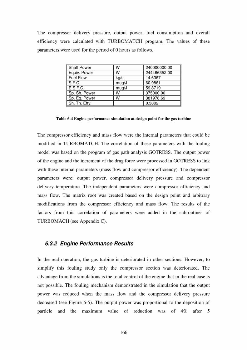
166
The compressor delivery pressure, output power, fuel consumption and overall
efficiency were calculated with TURBOMATCH program. The values of these
parameters were used for the period of 0 hours as follows.
Shaft Power W 240000000.00
Equiv. Power W 244466352.00
Fuel Flow kg/s 14.6367
S.F.C. mug/J 60.9861
E.S.F.C. mug/J 59.8719
Sp. Sh. Power W 375000.00
Sp. Eq. Power W 381978.69
Sh. Th. Effy. 0.3802
Table 6-4 Engine performance simulation at design point for the gas turbine
The compressor efficiency and mass flow were the internal parameters that could be
modified in TURBOMATCH. The correlation of these parameters with the fouling
model was based on the program of gas path analysis GOTRESS. The output power
of the engine and the increment of the drag force were processed in GOTRESS to link
with these internal parameters (mass flow and compressor efficiency). The dependent
parameters were: output power, compressor delivery pressure and compressor
delivery temperature. The independent parameters were compressor efficiency and
mass flow. The matrix root was created based on the design point and arbitrary
modifications from the compressor efficiency and mass flow. The results of the
factors from this correlation of parameters were added in the subroutines of
TURBOMACH (see Appendix C).
6.3.2 Engine Performance Results
In the real operation, the gas turbine is deteriorated in other sections. However, to
simplify this fouling study only the compressor section was deteriorated. The
advantage from the simulations is the total control of the engine that in the real case is
not possible. The fouling mechanism demonstrated in the simulation that the output
power was reduced when the mass flow and the compressor delivery pressure
decreased (see Figure 6-5). The output power was proportional to the deposition of
particle and the maximum value of reduction was of 4% after 5
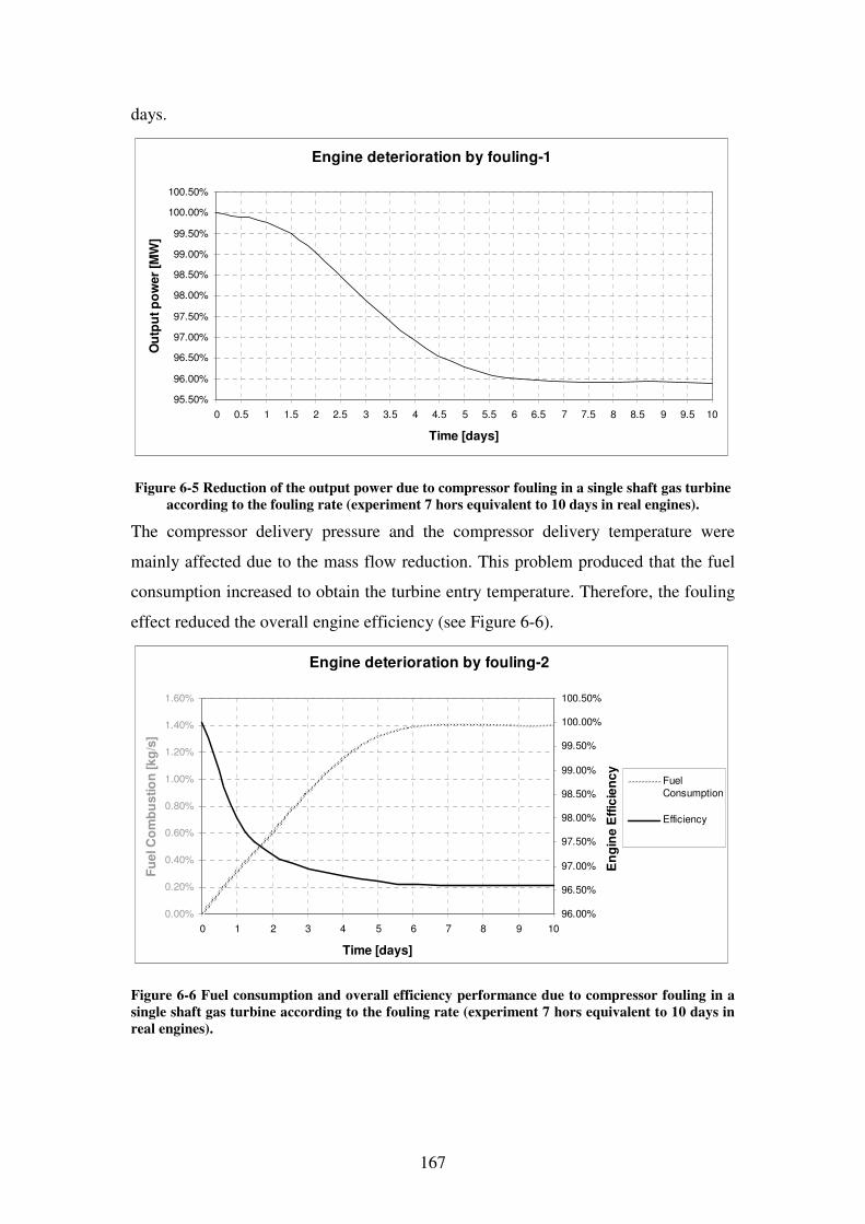
167
days.
Engine deterioration by fouling-1
95.50%
96.00%
96.50%
97.00%
97.50%
98.00%
98.50%
99.00%
99.50%
100.00%
100.50%
0 0.5 1 1.5 2 2.5 3 3.5 4 4.5 5 5.5 6 6.5 7 7.5 8 8.5 9 9.5 10
Time [days]
Ou
tpu
t p
ow
er
[MW
]
Figure 6-5 Reduction of the output power due to compressor fouling in a single shaft gas turbine
according to the fouling rate (experiment 7 hors equivalent to 10 days in real engines).
The compressor delivery pressure and the compressor delivery temperature were
mainly affected due to the mass flow reduction. This problem produced that the fuel
consumption increased to obtain the turbine entry temperature. Therefore, the fouling
effect reduced the overall engine efficiency (see Figure 6-6).
Engine deterioration by fouling-2
0.00%
0.20%
0.40%
0.60%
0.80%
1.00%
1.20%
1.40%
1.60%
0 1 2 3 4 5 6 7 8 9 10
Time [days]
Fu
el C
om
bu
stio
n [
kg
/s]
96.00%
96.50%
97.00%
97.50%
98.00%
98.50%
99.00%
99.50%
100.00%
100.50%
En
gin
e E
ffic
ien
cy
Fuel
Consumption
Efficiency
Figure 6-6 Fuel consumption and overall efficiency performance due to compressor fouling in a
single shaft gas turbine according to the fouling rate (experiment 7 hors equivalent to 10 days in
real engines).
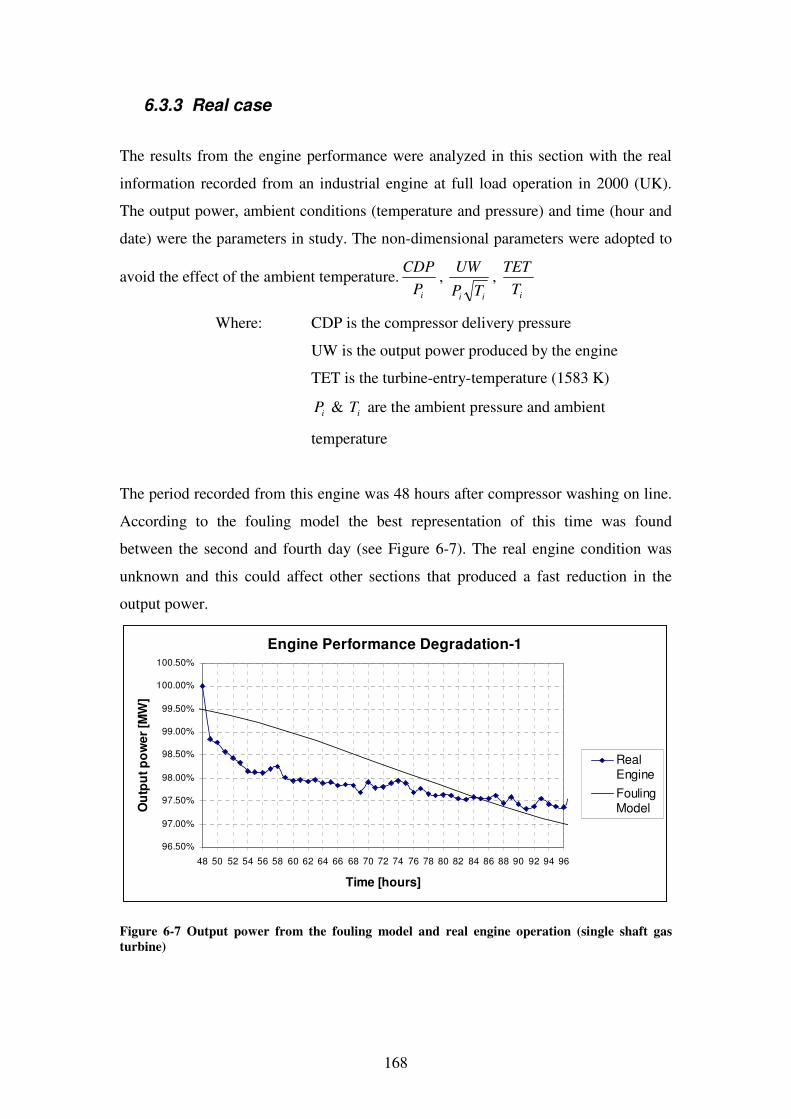
168
6.3.3 Real case
The results from the engine performance were analyzed in this section with the real
information recorded from an industrial engine at full load operation in 2000 (UK).
The output power, ambient conditions (temperature and pressure) and time (hour and
date) were the parameters in study. The non-dimensional parameters were adopted to
avoid the effect of the ambient temperature.iP
CDP,
ii TP
UW,
iT
TET
Where: CDP is the compressor delivery pressure
UW is the output power produced by the engine
TET is the turbine-entry-temperature (1583 K)
iP & iT are the ambient pressure and ambient
temperature
The period recorded from this engine was 48 hours after compressor washing on line.
According to the fouling model the best representation of this time was found
between the second and fourth day (see Figure 6-7). The real engine condition was
unknown and this could affect other sections that produced a fast reduction in the
output power.
Engine Performance Degradation-1
96.50%
97.00%
97.50%
98.00%
98.50%
99.00%
99.50%
100.00%
100.50%
48 50 52 54 56 58 60 62 64 66 68 70 72 74 76 78 80 82 84 86 88 90 92 94 96
Time [hours]
Ou
tpu
t p
ow
er
[MW
]
RealEngine
FoulingModel
Figure 6-7 Output power from the fouling model and real engine operation (single shaft gas
turbine)
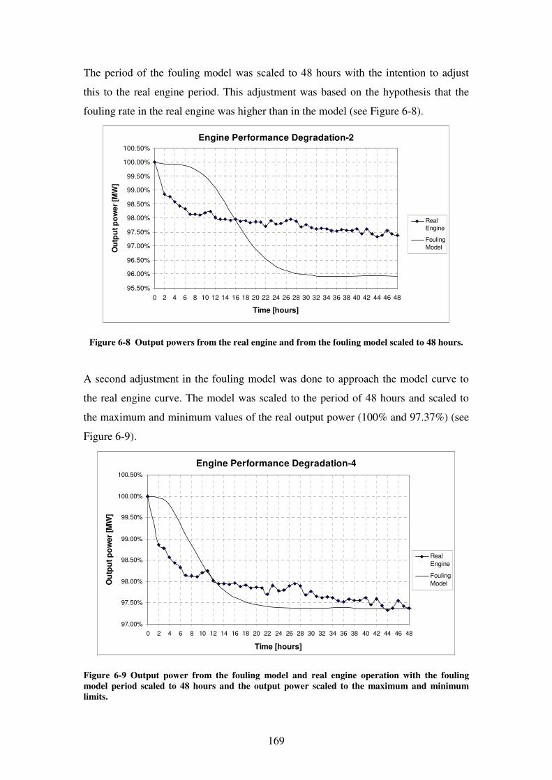
169
The period of the fouling model was scaled to 48 hours with the intention to adjust
this to the real engine period. This adjustment was based on the hypothesis that the
fouling rate in the real engine was higher than in the model (see Figure 6-8).
Engine Performance Degradation-2
95.50%
96.00%
96.50%
97.00%
97.50%
98.00%
98.50%
99.00%
99.50%
100.00%
100.50%
0 2 4 6 8 10 12 14 16 18 20 22 24 26 28 30 32 34 36 38 40 42 44 46 48
Time [hours]
Ou
tpu
t p
ow
er
[MW
]
Real
Engine
Fouling
Model
Figure 6-8 Output powers from the real engine and from the fouling model scaled to 48 hours.
A second adjustment in the fouling model was done to approach the model curve to
the real engine curve. The model was scaled to the period of 48 hours and scaled to
the maximum and minimum values of the real output power (100% and 97.37%) (see
Figure 6-9).
Engine Performance Degradation-4
97.00%
97.50%
98.00%
98.50%
99.00%
99.50%
100.00%
100.50%
0 2 4 6 8 10 12 14 16 18 20 22 24 26 28 30 32 34 36 38 40 42 44 46 48
Time [hours]
Ou
tpu
t p
ow
er
[MW
]
Real
Engine
Fouling
Model
Figure 6-9 Output power from the fouling model and real engine operation with the fouling
model period scaled to 48 hours and the output power scaled to the maximum and minimum
limits.
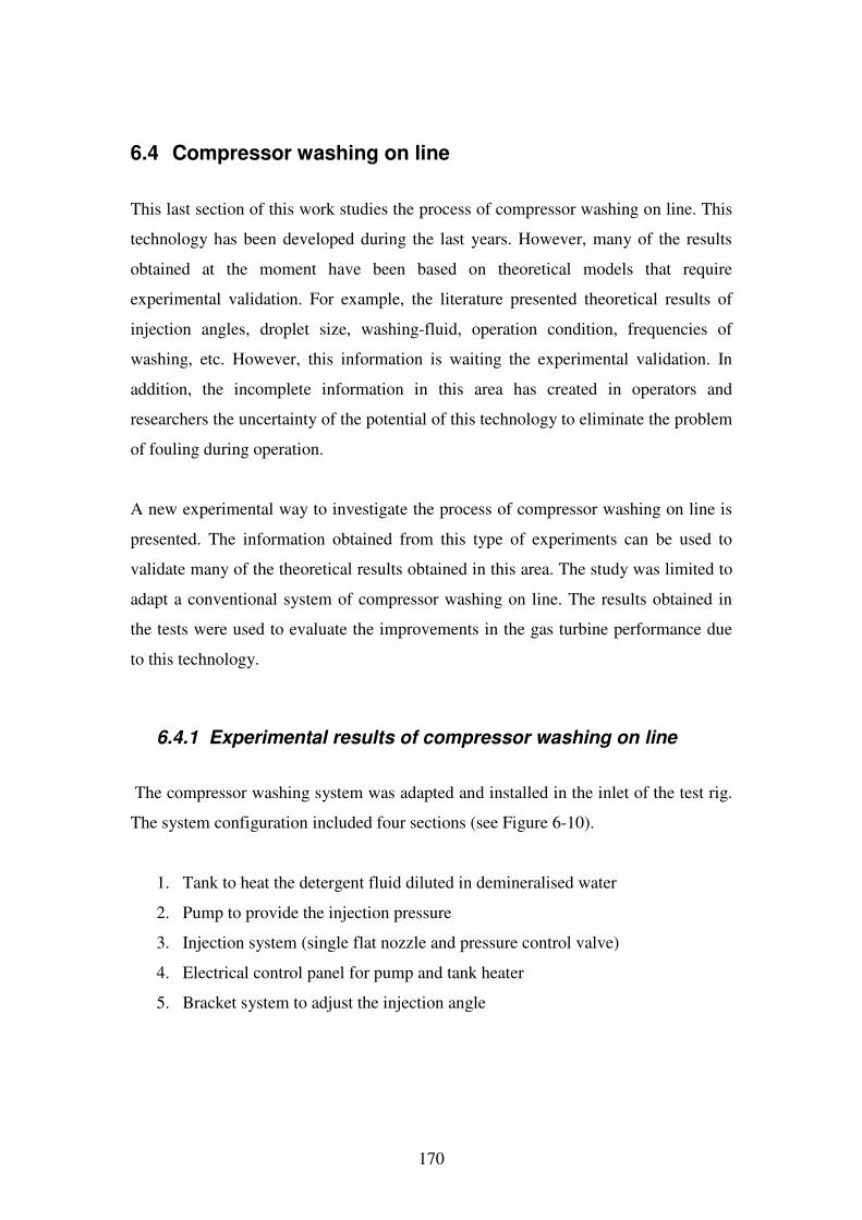
170
6.4 Compressor washing on line
This last section of this work studies the process of compressor washing on line. This
technology has been developed during the last years. However, many of the results
obtained at the moment have been based on theoretical models that require
experimental validation. For example, the literature presented theoretical results of
injection angles, droplet size, washing-fluid, operation condition, frequencies of
washing, etc. However, this information is waiting the experimental validation. In
addition, the incomplete information in this area has created in operators and
researchers the uncertainty of the potential of this technology to eliminate the problem
of fouling during operation.
A new experimental way to investigate the process of compressor washing on line is
presented. The information obtained from this type of experiments can be used to
validate many of the theoretical results obtained in this area. The study was limited to
adapt a conventional system of compressor washing on line. The results obtained in
the tests were used to evaluate the improvements in the gas turbine performance due
to this technology.
6.4.1 Experimental results of compressor washing on line
The compressor washing system was adapted and installed in the inlet of the test rig.
The system configuration included four sections (see Figure 6-10).
1. Tank to heat the detergent fluid diluted in demineralised water
2. Pump to provide the injection pressure
3. Injection system (single flat nozzle and pressure control valve)
4. Electrical control panel for pump and tank heater
5. Bracket system to adjust the injection angle
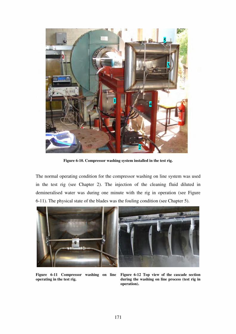
171
Figure 6-10. Compressor washing system installed in the test rig.
The normal operating condition for the compressor washing on line system was used
in the test rig (see Chapter 2). The injection of the cleaning fluid diluted in
demineralised water was during one minute with the rig in operation (see Figure
6-11). The physical state of the blades was the fouling condition (see Chapter 5).
Figure 6-11 Compressor washing on line
operating in the test rig.
Figure 6-12 Top view of the cascade section
during the washing on line process (test rig in
operation).
1
5
4
3
2
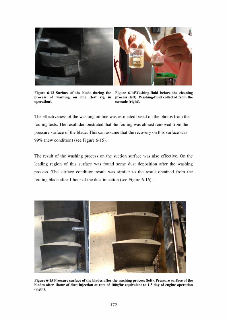
172
Figure 6-13 Surface of the blade during the
process of washing on line (test rig in
operation).
Figure 6-14Washing-fluid before the cleaning
process (left). Washing-fluid collected from the
cascade (right).
The effectiveness of the washing on line was estimated based on the photos from the
fouling tests. The result demonstrated that the fouling was almost removed from the
pressure surface of the blade. This can assume that the recovery on this surface was
99% (new condition) (see Figure 6-15).
The result of the washing process on the suction surface was also effective. On the
leading region of this surface was found some dust deposition after the washing
process. The surface condition result was similar to the result obtained from the
fouling blade after 1 hour of the dust injection (see Figure 6-16).
Figure 6-15 Pressure surface of the blades after the washing process (left). Pressure surface of the
blades after 1hour of dust injection at rate of 100g/hr equivalent to 1.5 day of engine operation
(right).
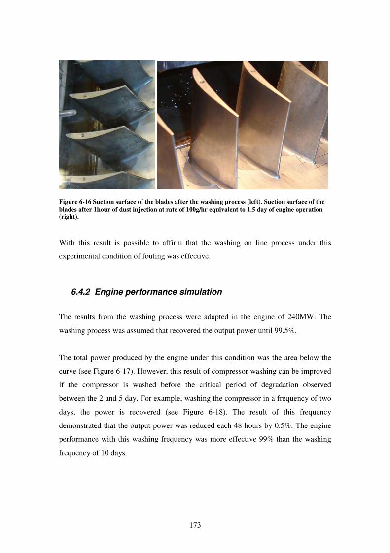
173
Figure 6-16 Suction surface of the blades after the washing process (left). Suction surface of the
blades after 1hour of dust injection at rate of 100g/hr equivalent to 1.5 day of engine operation
(right).
With this result is possible to affirm that the washing on line process under this
experimental condition of fouling was effective.
6.4.2 Engine performance simulation
The results from the washing process were adapted in the engine of 240MW. The
washing process was assumed that recovered the output power until 99.5%.
The total power produced by the engine under this condition was the area below the
curve (see Figure 6-17). However, this result of compressor washing can be improved
if the compressor is washed before the critical period of degradation observed
between the 2 and 5 day. For example, washing the compressor in a frequency of two
days, the power is recovered (see Figure 6-18). The result of this frequency
demonstrated that the output power was reduced each 48 hours by 0.5%. The engine
performance with this washing frequency was more effective 99% than the washing
frequency of 10 days.
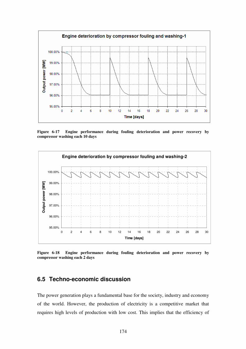
174
Figure 6-17 Engine performance during fouling deterioration and power recovery by
compressor washing each 10 days
Engine deterioration by compressor fouling and washing-2
95.00%
96.00%
97.00%
98.00%
99.00%
100.00%
0 2 4 6 8 10 12 14 16 18 20 22 24 26 28 30
Time [days]
Ou
tpu
t p
ow
er
[MW
]
Figure 6-18 Engine performance during fouling deterioration and power recovery by
compressor washing each 2 days
6.5 Techno-economic discussion
The power generation plays a fundamental base for the society, industry and economy
of the world. However, the production of electricity is a competitive market that
requires high levels of production with low cost. This implies that the efficiency of
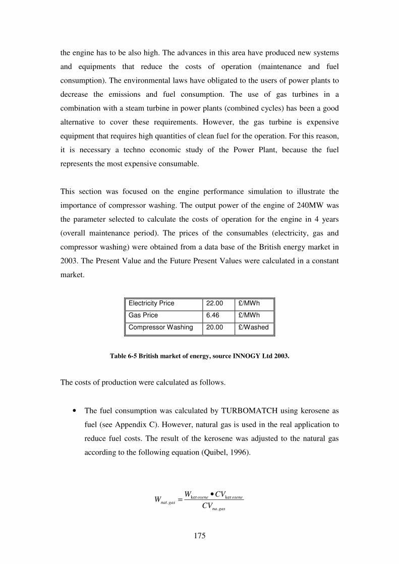
175
the engine has to be also high. The advances in this area have produced new systems
and equipments that reduce the costs of operation (maintenance and fuel
consumption). The environmental laws have obligated to the users of power plants to
decrease the emissions and fuel consumption. The use of gas turbines in a
combination with a steam turbine in power plants (combined cycles) has been a good
alternative to cover these requirements. However, the gas turbine is expensive
equipment that requires high quantities of clean fuel for the operation. For this reason,
it is necessary a techno economic study of the Power Plant, because the fuel
represents the most expensive consumable.
This section was focused on the engine performance simulation to illustrate the
importance of compressor washing. The output power of the engine of 240MW was
the parameter selected to calculate the costs of operation for the engine in 4 years
(overall maintenance period). The prices of the consumables (electricity, gas and
compressor washing) were obtained from a data base of the British energy market in
2003. The Present Value and the Future Present Values were calculated in a constant
market.
Electricity Price 22.00 £/MWh
Gas Price 6.46 £/MWh
Compressor Washing 20.00 £/Washed
Table 6-5 British market of energy, source INNOGY Ltd 2003.
The costs of production were calculated as follows.
• The fuel consumption was calculated by TURBOMATCH using kerosene as
fuel (see Appendix C). However, natural gas is used in the real application to
reduce fuel costs. The result of the kerosene was adjusted to the natural gas
according to the following equation (Quibel, 1996).
gasna
oseneosene
gasnatCV
CVWW
.
kerker.
•=
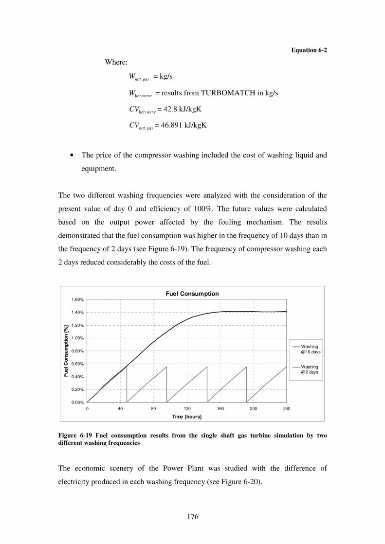
176
Equation 6-2
Where:
gasnatW . = kg/s
oseneWker = results from TURBOMATCH in kg/s
oseneCVker = 42.8 kJ/kgK
gasnatCV . = 46.891 kJ/kgK
• The price of the compressor washing included the cost of washing liquid and
equipment.
The two different washing frequencies were analyzed with the consideration of the
present value of day 0 and efficiency of 100%. The future values were calculated
based on the output power affected by the fouling mechanism. The results
demonstrated that the fuel consumption was higher in the frequency of 10 days than in
the frequency of 2 days (see Figure 6-19). The frequency of compressor washing each
2 days reduced considerably the costs of the fuel.
Fuel Consumption
0.00%
0.20%
0.40%
0.60%
0.80%
1.00%
1.20%
1.40%
1.60%
0 40 80 120 160 200 240
Time [hours]
Fu
el C
on
su
mp
tio
n [
%]
Washing
@10 days
Washing
@2 days
Figure 6-19 Fuel consumption results from the single shaft gas turbine simulation by two
different washing frequencies
The economic scenery of the Power Plant was studied with the difference of
electricity produced in each washing frequency (see Figure 6-20).
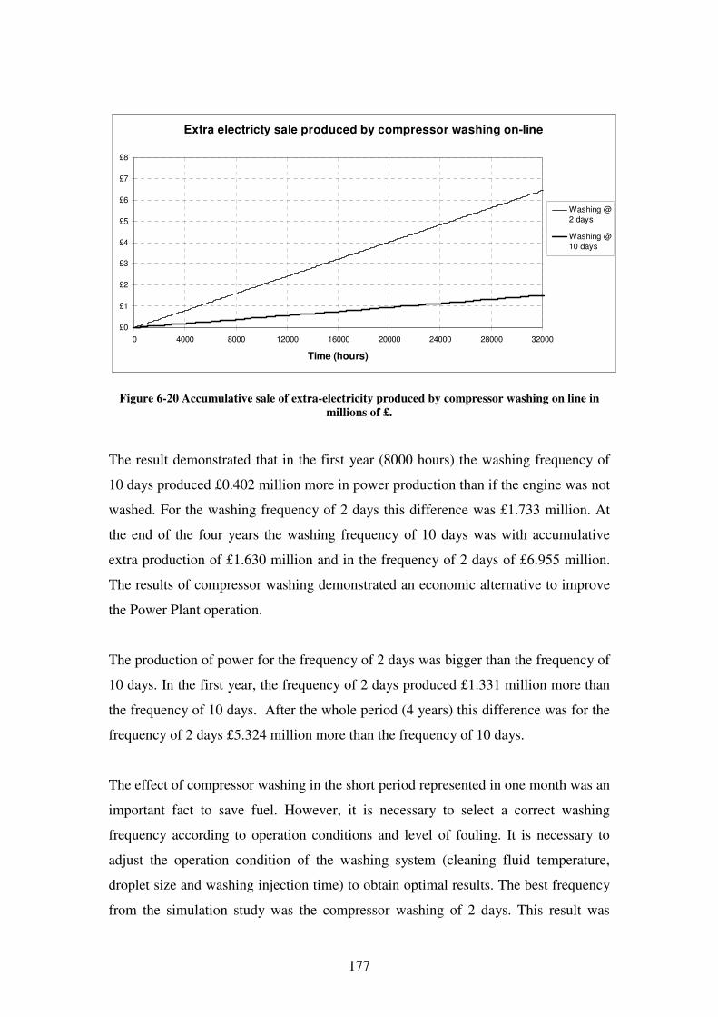
177
Extra electricty sale produced by compressor washing on-line
£0
£1
£2
£3
£4
£5
£6
£7
£8
0 4000 8000 12000 16000 20000 24000 28000 32000
Time (hours)
Washing @
2 days
Washing @
10 days
Figure 6-20 Accumulative sale of extra-electricity produced by compressor washing on line in
millions of £.
The result demonstrated that in the first year (8000 hours) the washing frequency of
10 days produced £0.402 million more in power production than if the engine was not
washed. For the washing frequency of 2 days this difference was £1.733 million. At
the end of the four years the washing frequency of 10 days was with accumulative
extra production of £1.630 million and in the frequency of 2 days of £6.955 million.
The results of compressor washing demonstrated an economic alternative to improve
the Power Plant operation.
The production of power for the frequency of 2 days was bigger than the frequency of
10 days. In the first year, the frequency of 2 days produced £1.331 million more than
the frequency of 10 days. After the whole period (4 years) this difference was for the
frequency of 2 days £5.324 million more than the frequency of 10 days.
The effect of compressor washing in the short period represented in one month was an
important fact to save fuel. However, it is necessary to select a correct washing
frequency according to operation conditions and level of fouling. It is necessary to
adjust the operation condition of the washing system (cleaning fluid temperature,
droplet size and washing injection time) to obtain optimal results. The best frequency
from the simulation study was the compressor washing of 2 days. This result was

178
close to the empirical period of washing 3 times per week suggested by the
compressor washing manufacturers. However, this value was not definitive, because it
was based for an engine in new condition. Then, it is important to evaluate first the
engine condition to find the optimal washing frequency. The possibility to combine
different frequencies of washing could result an effective technique when the
concentration of particles in the air changes.
179
7 CONCLUSION AND RECOMMENDATIONS
7.1 Conclusion
This last chapter discusses the results obtained by this research based on the
experimental study of the fouling mechanism in compressor blades. The model
presented in this investigation was created according to the experimental and CFD
results. The information obtained from the test rig was validated with the CFD model
and with real gas turbines data. The conclusions are presented according to the thesis
order.
According to the literature review, the main mechanism of degradation in the
compressor is the phenomenon of fouling. This is an evident problem that affects the
compressor performance and overall efficiency of the gas turbine. A detailed
recompilation of information about the possible sources of fouling was presented in this
work. Also, the effect of fouling in a different engine configuration was analyzed. The
engine configuration of a single shaft demonstrated to be a complicate job to detect the
fouling problem. This is because the engine components in the single shaft are attached
to the same shaft and then the problem is hidden by the performance of the components.
In Chapter 2 was found that many authors coincided that fouling reduces the overall
engine efficiency by 5%. However, this result was created based on arbitrary factors
calculated only from the engine output power.
The originality of this work was the use of a test rig to study the effect of fouling in the
blade aerodynamics. The complete methodology for the design and building of the test
rig and cascade section was presented in this work. The conditions reproduced in the
test rig were based on the inlet conditions of a first axial compressor. The geometrical
dimension for the real blade size was reproduced in the experiment. The cascade section
from the test rig was designed to reproduce uniform flow. The final test rig
configuration was the result of three modifications from the original configuration. The
condition of the flow was calculated by a CFD model. The application of the CFD was a
successful tool to study the physical phenomenon only when the boundary conditions
180
were known. In this case, the boundary conditions were the atmospheric conditions and
the static pressure of the outlet cascade. An internal parameter was used to adjust the
model (static pressure of cascade inlet). The use of the real values from the outlet of the
cascade in the CFD simulations was not successful. Therefore, the outlet boundary
condition was modified from the original values to approach the CFD results to the
internal parameter.
The key to reproduce uniform flow inside the cascade was in this case the shape of the
side walls. The shape of the walls was designed according to the blade exit angle. This
conclusion contrasts with the idea to have several blades in the cascade row mentioned
in the literature review. The selection of the materials also played an important role in
the design. The use of aluminium was a correct selection to build the test rig. However,
the “plexi-glass” selected presented several problems since the machine process and
later on in the modifications.
The instrumentation used in the experiment presented two limitations. The first was the
collection of information in a high Mach numbers (Ma=0.7). And for that reason, the
study was based in a low flow velocities (Ma=0.25). The second limitation was the
ability to study the boundary layer. This limitation was mentioned in the literature
review because the boundary layer involved the micro scale as was demonstrated in this
research. Therefore, the boundary layer region was studied exclusive from the
application of the CFD. The thermocouples and surface roughness instruments resulted
a correct selection to record the experimental data.
The study region was selected in the central passage of the cascade (between the 2nd and
3rd blade). This was due to present the best flow uniformity in the cascade. The cascade
was designed for two dimensional studies. The horizontal plane at the middle blade
height was analyzed with the experimental techniques of flow visualization. The oxide
of titanium used to visualize the flow path was a successful technique to track the flow
path. This result showed the evidence that the flow was travelling in two dimensional
trajectories and the three dimensional flow effects was nil. With these two results it was
possible to conclude that the flow trajectory was not affected by the top or bottom of the
181
cascade. In addition, the design of the damper diffusion section at the rig outlet was
correct and avoided flow fluctuation produced by the vortex induced in the inlet of the
fan.
An important contribution from the CFD in this research was the calculations of
parameters that were not possible to measure with the instrumentation available. The
two main parameters calculated by the CFD were the static pressure distribution on the
blade surface and the boundary layer region. The CFD had to be adjusted and calibrated
according to the experimental information from the macro-scale. The parameter used as
a criterion to evaluate the CFD model was the geometrical localization of the blade
wake. This was a successful result, because the geometrical location of the wake in the
test rig coincided with the CFD result. The conclusion was that the results from the
CFD are considered reliable in this investigation.
This work is pioneering in the study of fouling and for that reason it was necessary to
cover the lack of information missing about this topic. The first problem was to
establish the condition of the blade surface. The information regarding the blade surface
roughness was limited and it obligated to make a field investigation in real blades. The
final result was to adopt the value of Ra =0.6 µm for the roughness surface of the
blades. This value was obtained from new blades delivered directly from the OEM. A
second problem was the information about the fouling conditions. This information was
covered with the data and dust sample provided from the company Recovery Power
Ltd. The dust injection rate was calculated with the information and data recorded in the
technical visit to Didcot Power Plant. The flow velocity in the cascade was assumed
constant and the calculations resulted in a rate of dust injection of 2.8 g/h. The process
of fouling was accelerated under two main hypotheses. 1 hour of the experimental dust
injection rate was equivalent to 1.5 days of the real operation. The second factor was the
use of a glue-agent to increase the particle deposition on the blade surface. These two
factors were tested with an artificial powder to evaluate the fouling results in the test rig.
The results from the experimental fouling were close to the fouling observed from the
real IGV of the engines. This effect was the result of the static conditions in the cascade.
182
In this case, the experimental blades represented static airfoils. The most important
result from the experiment was the possibility to reproduce and record the progressive
formation of fouling. With this information was found that the fouling on the blade was
non-uniform. This mechanism is a complex phenomenon that involves the aerodynamic
shape of the blade and the rate of fouling. In addition, the blade surface presented
regions with roughness increments on the pressure surface of 80µm and on the suction
surface of 97µm.
The application of the fouling model resulted in eight sections that represent different
regions of the blade surface. However, this model was not practical to evaluate the
engine performance and it was necessary to link this with other parameters using the
CFD model. The parameters of static pressure and friction skin coefficient were
calculated. The fouling effect in these parameters was observed only on the suction
surface. Then, a third parameter was calculated to include the whole blade profile. This
was the difference of the blade drag when fouling was presented. The result of the drag
was used to estimate the fouling effect in the engine performance. The values were
scaled to the blade height and processed in GOTRESS to predict the factors that
decreased the mass flow and the compressor efficiency. The factors were inserted in the
code of TURBOMATCH to calculate the engine performance.
The results of the engine simulation in TURBOMATCH demonstrated that the engine
efficiency decreased in a period of 5 days by 3.5%. The engine performance was
affected since the first day of operation due to the particles deposition. This was
favoured when the smooth surface was presented. According to the results of this
simulation, the problem of fouling could affect directly the overall efficiency until 3.5%
only. However, in the real application this problem could be transmitted to other section
and increases the reduction of the overall efficiency. The results of the engine
performance were compared with real data from an engine in operation. The simulation
result was adjusted according to the time and output power limits by linear factors. This
arbitrary modification in the model was based on the hypothesis that the real engine was
affected by higher concentration of particles in the flow. The conclusion of this
183
adjustment was that that the engine performance of the model resulted almost similar to
the performance of the real engine.
The last section of this research was focused to study the compressor washing on line.
The experimental results demonstrated that the process of washing removed almost
completely the fouling on the blade. The recovery of the engine power was calculated
with TURBOMATCH based on an economical scenario of a gas turbine in operation
during four years in a Power Plant. The conclusion of this study was that compressor
washing on line is an economic and technical solution to recover the power lost due to
fouling. In this case of an engine of 240MW the power recovered in four years is
equivalent to £6.5 million of electricity sale.
This thesis has covered the objective to create a preliminary model to predict the fouling
formation based on experimental tests. The experimental and CFD models resulted a
successful way to study the fouling problem and two main conclusions summarize these
results. First, the mechanism of fouling is non linear to the time and also is non-uniform
on the surface of the blade. The experimental result identified that the critical region of
particle deposition is the leading edge of the blade. With this information it was possible
to calculate the aerodynamics blade changes and evaluate the effect of fouling in the
engine performance. The second conclusion was the effectiveness of the compressor
washing on line system to eliminate the fouling problem. Finally, this work has included
an overall study of fouling in the study and development of gas turbines.
7.2 Recommendations
In this section is presented the research limitations and the possible recommendations
for further investigations in this area. Basically, there are three important considerations
that further investigations should be considered before to generalize the application of
the fouling model presented in this study. The first one regards the study of the blade
profile. Because, the fouling result was based on an exclusive blade profile and the dust
deposition could be different from another condition of dust injection rate. The second
184
regards to the dust type and the third regards to the specific flow condition used (flow
velocity).
The use of this particular test rig can be extended for other blades that fix in the cascade
the test rig. It is recommended that the blades be located in the centre of the cascade
section, so that they are more clearly visible. Also, the use of small blades can increase
the number of blades and passages.
For new designs it is essential to consider the characteristics of the power source. The
configuration of the fan (blow or suck) depends on the study region selected. In this
particular work the blade inlet conditions was selected. Using the fan configuration to
(blowing) could give a criterion to decide which configuration is the most appropriate.
Another aspect is the material selection for the test rig. It is recommendable to avoid the
use of “plexy glass” in sections that requires complex manufacture (aerodynamic
shapes) or for main body sections (frames). This material is fragile and difficult for
manufacturing process. The use of aluminium is suggested because it is light and easy
to manufacture. The test rig is recommendable to be designed in modules. The use of
star-bolts and brackets in each section presents a good alternative in the joint of
sections.
The CFD was essential in this investigation to calculate the parameters that were not
possible to measure in the experiment. However, it is important to have in mind the
limitations of the CFD, because each result represents a possible solution that will be
judged by the researcher and for that reason it is highly recommended to have a solid
criterion of the physical phenomenon based on experimental or real data. This
information also will help to adjust the CFD model as it was in this case the macro scale
information used to validate and adjust the CFD model. The computational time to
process the information is another parameter to consider because this can represent a
serious problem when a high precise solution is required. It is suggested to increase
gradually the process of the CFD since very basic to complex models. Following this
suggestion, it is possible to detect an error during the early stages and avoid long
periods of time for incorrect or non-converged solutions.

185
The results of this research were studied in two dimensional conditions. However, to
cover the whole area, it will be necessary to study the rotational effect of the flow. The
three dimensional deposition of the dust in the CFD represents a new challenger to
investigate. One of the most important applications of the CFD is the possibility of
simulating the flow in the whole compressor. So, further investigations could give an
important result in studies that includes each particular stage of the compressor. Also,
the simulation of the mechanism of fouling by CFD represents a challenge for future
investigations. In addition, the compressor washing on line should be analyzed with
different fouling samples and this possibility could be studied in the test rig of this
investigation.
The results of this investigation can be used as a guide of new projects. The real status
of the compressor can only be understood with complete and solid background
knowledge of the fouling phenomenon. The future information of compressor washing
will result important in the total elimination of fouling.
186
REFERENCES
Abdelrazik, A. and Cheney, P. (1991), Compressor cleaning effectiveness for marine gas turbines, Conference: International Gas Turbine and Aeroengine Congress and Exposition, Jun 3-6 1991, pp. 6.
Aker, G. and Saravanamuttoo, H. (1989), Predicting gas turbine performance degradation due to compressor fouling using computer simulation techniques, Journal of Engineering for Gas Turbines and Power, Transactions of the ASME, Vol. 111, No. 2, pp. 343-350.
Asplund, P. (1998), Gas turbine cleaning upgrade’ (compressor wash), VTT Symposium (Valtion Teknillinen Tutkimuskeskus), Vol. 184, pp. 105.
Bagshaw K.W. (1974), Maintaining Cleanliness in Axial Compressor (National Research Council edition), Canada.
Barlow, H., Rae, W., and Pope, A. (1999), Low speed tunnel testing (3rd edition), New York.
Bouris, D., Kubo, R., Hirata, H., and Nakata, Y. (2002), Numerical comparative study of compressor rotor and stator blade deposition rates, Journal of Engineering for Gas Turbines and Power, Vol. 124, No. 3, pp. 608-616.
Boyce, M. P., Bowman, J. C., Meher-Homji, C., and Focke, A. B. (1985), Energy efficient operation of gas turbine compressor sets, Gas Turbine Conference, USA.
Boyce, M. and Gonzalez, F. (2005), A study of on-line and off-line turbine washing to optimize the operation of a gas turbine, ASME Turbo Expo 2005.*
Britchford, K., Manners, A., McGuirk, J., and Stevens, S. (1994), Measurement and prediction of flow in annular S-shaped ducts, Experimental Thermal and Fluid Science, Vol. 9, No. 2, pp. 197-205.
Brittain, D. (1983), Cleaning gas turbine compressors, Aircraft Engineering.
Brooks, F. J. (2000), GE Gas Turbine Performance Characteristics, GE Report.
Brumbaugh, D. (2002), Inlet air filtration adapts to evolving gas turbine technology, Power Engineering, Vol. 106, No. 10, pp. 51-54.
Caguiat, D., Zipkin, D. M., and Patterson, J. (2002), Compressor fouling testing on Rolls Royce/Allison 501-K17 and general electric LM2500 gas turbine engines, American Society of Mechanical Engineers Turbo Expo 2002, Vol. 2, No. B, pp. 933-942.
Caguiat, D. E. (2003), Rolls Royce/Allison 501-K gas turbine antifouling compressor coatings evaluation, Journal of Turbomachinery, Vol. 125, No. 3, pp. 482-488.
Caterpillar (2005), Power Solar Turbines, available at: www.solarturbines.com
Diakunchak, I. S. (1991), Performance deterioration in industrial gas turbines (International Gas Turbine and Aero-engine Congress and Exposition jun 3-6 edition), New York, USA.
Dixon, S. L. (1998), Fluid Mechanics and Thermodynamics of Turbomachinery (4th edition), Butterworth-Heinemann, USA.
Donaldson Company (2005), TTD Self Cleaning System (GTS -102 rev 6 edition), Donaldson Solution Company.
187
Escher, P. C. (1995), An Object Oriented Gas Path Analysis Computer Program for General Applications (PhD Thesis), Cranfield University, UK.
Farrel, D. M. and Vittal, B. V. R. (1996), Computer Simulation of Water Ingestion for the T800-LHT-801 Engine Anti-Icing Test Inlet, AIAA.
Fielder, J. (2003), Evaluation of zero compressor wash routine in RN service, 2003 ASME Turbo Expo, Vol. 3, pp. 543-547.
Flashberg, L. S. (1992), Measurement of combustion turbine non-recoverable degradation, International Exhibition & Conference for the Power Generation Industries.
Fluent Inc (2005), User's guide (version 6.2 Manual Edition edition), Fluent.
Freid, W. B. and Tapparo, D. J. (1971), Wash mnifold, USA Patent 3623668, USA.
Gahr, T., Benson, J., Graham, K., Gogins, M., and Brown, M. (2005), Advancements in electrospun nanofiber technology reduce gas turbine compressor fouling, ASME Turbo Expo 2005.*
Gbadebo, S. A., Hynes, T. P., and Cumpsty, N. A. (2004), Influence of surface roughness on three-dimensional separation in axial compressor, Journal of Turbomachinery, Vol. 4, No. 4, pp. 455-463.
General Electric (2001), Compressor rotor R-0 blade erosion, Technical Information Letter, GE Energy Services,
Giampolo, T. (1997), The Gas Turbine Handbook, The Fairmont Press, USA.
Gostelow, J. P. (1984), Cascade Aerodynamics, Pergamon Press Ltd, Australia.
Gulen, S., Griffin, P., and Paolucci, S. (2002), Real-time on-line performance diagnostics of heavy-duty industrial gas turbines, Journal of Engineering for Gas Turbines and Power, Vol. 124, No. 4, pp. 910-921.
Haq, I. and Saravanamuttoo, H. (1991), Detection of axial compressor fouling in high ambient temperature conditions, American Society of Mechanical Engineers , pp. 9.
Harris, H. and Calabrese, M. (1994), On-line detergent fluid evaluation on a TF4OB gas turbine engine, American Society of Mechanical Engineers, 94-GT-452, pp. 1-9.
Haub, G. and Hauhe, W. (1990), Field evaluation of on-line compressor cleaning in heavy duty industrial gas turbines, International Gas Turbine and Aeroengine Congress and Exposition, Jun 11-14 1990, Brussels, Belg, pp. 12.
Hobson, G., Hansen, D., Schnorenberg, D., and Grove, D. (2001), Effect of Reynolds number on separation bubbles on compressor blades in cascade, Journal of Propulsion and Power, Vol. 17, No. 1, pp. 154-162.
Hoeft, R. F. (1993), Heavy Duty Gas Turbine Operating and Maintenance Considerations, GE I&PS.
Howell, A. R. and Calvert, W. J. A. (1978), New Stage Stacking Technique for Axial Flow Compressor Performance Prediction, 100:698-703.
Ingistov, S. (2002), Interstage Injection into Axial Compressor, Gas Turbine Model 7EA, ASME Turbo Expo 2002.*
Jeffs, E. (1992), Compressor washing on line for large turbines, Turbomachinery International.
188
Jeffs, E. (2000), Siemens Cockpit 2000: Integrated plant management for the IPP, Turbomachinery International, Vol. 41, No. 4, pp. 16-17.
Kaes, G. (1991), Method of a cleaning agent for the cleaning compressors especially gas turbines, US Patent 5076855, USA.
Kolev, S. and Robben, R. (1993), Injection device for the on-line wet cleaning of compressors, US Patent 5193976, USA.
Kolkman, H. (1993), Performance of gas turbine compressor cleaners, : Journal of Engineering for Gas Turbines and Power, Transactions of the ASME, Vol. 115, No. 3, pp. 674-677.
Kulle, V. (1974), Gas turbine blade cleaning at Alberta gas trunk line (AGTL) (Gas Turbine Operation and Maintenance Symposium edition), In N.R.C. of Canada.
Kurz R. and Brun K. (2001), Degradation in gas turbine systems, Journal of Engineering for Gas Turbines and Power, Vol. 123, No. 1, pp. 70-77.
Lakshminarasimha, A., Boyce, M., and Meher-Homji, C. (1994), Modelling and analysis of gas turbine performance deterioration, Journal of Engineering for Gas Turbines and Power, Transactions of the ASME, Vol. 116, No. 1, pp. 46-52.
Lakshminarasimha, A. and Saravanamutto, H. (1986), Prediction of fouled compressor performance using stage stacking techniques, American Society of Mechanical Engineers, Fluids Engineering Division (Publication) FED, Vol. 37, pp. 59-66.
Lambart, P., Gordon, R., and Burnett, M. (2003), Developments in on-line gas turbine cleaning, Institution of Diesel and Gas Turbine Engineers 2nd Gas Turbine Conference, UK.
Langford, J. L. F. (1977), Contamination removal method, Patent 4,065,322, USA.
Leusden, C. P., Sorgenfrey, C., and Dummel, L. ( 2003), Performance benefits using Siemens advanced compressor cleaning system, Germany (Siemens AG Power Generation), Vol. 1 at Atlanta, Georgia, USA; American Society of Mechanical Engineers, USA, pp. 793-801.
Levine, P. and Angello, L. (2005), Axial Compressor Performance Maintenance, ASME Turbo Expo 2005.*
Mansson, M. Washing apparatus for a compound compressor, USA Patent 4046155, USA.
Margolis, H. (1991), U.S. navy on-line compressor washing of marine gas turbine engines, International Gas Turbine and Aeroengine Congress and Exposition, Jun 3-6 1991, Orlando, FL, USA, pp. 6.
Mathioudakis, K., Stamatis, A., Tsalavoutas, A., and Aretakis, N. (2001), Performance analysis of industrial gas turbines for engine condition monitoring, Journal of Power and Energy, Vol. 215, No. 2, pp. 173-784.
Mathioudakis, K. and Tsalavoutas T. (2002), Uncertainly Reduction in Gas turbine Performance Diagnosis by Accounting for Humidity effects, Journal of Engineering for Gas Turbines and Power, Vol. 124, pp. 801808.
Mayle, R. E. (1991), Role of laminar-turbulent transition in gas turbine engines (Congress and Exposition ASME edition), USA.
McDermott, P. (1991), Gas turbine compressor fouling. The case for on-line cleaning, Turbomachinery International, Vol. 32, No. 1, pp. 34-38.
189
Meher-Homji and Cyrus B (1990), Gas turbine axial compressor fouling, a unified treatment of its effects, detection, and control, 1990 ASME COGEN-TURBO: 4th International Symposium on Gas Turbines in Cogeneration, Repowering, and Peak-Load Power Generation, Aug 27-29 1990, New Orleans, LA, USA, Vol. 5, pp. 179-190.
Meher-Homji, C. B. and Bromley, A. (2004), Gas Turbine Axial Compressor Fouling and Washing (33rd Turbomachinery Symposium edition), Texas A&M University, USA.
Mezheritsky, A. and Sudarev, A. (1990), Mechanism of fouling and the cleaning technique in application to flow parts of the power generation plant compressors, International Gas Turbine and Aeroengine Congress and Exposition, Jun 11-14 1990, Brussels, Belg , pp. 13.
Morillo De Hart, L. (1994), Performance Diagnostic of RR Avon Engines Using Gas Path Analysis, (MSc Thesis), Cranfield University, UK.
Mund, F. and Pilidis, P. (2004), A review of gas turbine online washing systems, Turbo Expo 2004.*
Mund, F. (2006), Coordinated Application of CFD and Gas Turbine Performance Methods (PhD Thesis), Cranfield University, UK.
Murthy, S. N. B., Ehresman, C. M. N., and Haykin, T. (1986), Direct and system effects of water ingestion into jet engine compressors, American Society of Mechanical Engineering - Fluids Engineering Division,
Mustafa, Z. (2006), Analysis of Droplets in Compressor Gas Turbines (PhD Thesis), Cranfield University, UK.
Olhovsky, G. G. (1985), Power Gas Turbine Unit, Moscow.
Orsach, R., Kazcprzynski, G., Roemer, M., Scharschan, J., Caguiat, D., and McGroarty, J. (2002), Applications of diagnostic algorithms for maintenance optimization of marine gas turbines, ASME TURBO EXPO 2002, Vol. 2, No. B, pp. 1025-1033.
Osborne, R. (1977), Design of an Industrial Gas Turbine Intake, American Air Filter Co.
Pankhurts, R. C. (1952), Wind-Tunnel Technique. An account of experimental methods in low and high speed tunnels, Sir Isaac Pitman & Sons, UK.
Peltier, R. and Swanekamp, R. (1995), LM2500 recoverable and non-recoverable power loss, American Society of Mechanical Engineers, 95-CTP-104, pp. 6.
Quibel, A. (1996), Performance and Deterioration Diagnostics of a 25 MW Turbine Plant at an Oil Refinery (MSc Thesis), Cranfield University, UK.
Ramsden, K. (2002), Axial Compressor Design and Performance Notes, Cranfield University, UK
Ramson, W. (2004), Adiabatic Effectiveness Measurements of Leakage Flows near the Hub Region of Gas Turbine Engines (MSc Thesis), Virginia Polithecnique Institute and State University, 2004.
Raykowski, A., Hader, M., Maragno, B., and Spelt, J. (2001), Blast cleaning of gas turbine components deposit removal and substrate deformation, Wear, Vol. 249, No. 1-2, pp. 127-132.
Razak, A. M. Y. and Dosanjh, M. S. (2002), Application of an advanced performance monitoring system to detect an implanted fault on a twin spool aero derived gas turbine, Gas Path Analysis Ltd., R. M. E. T. U. UK, Vol. 2 A at Amsterdam, The Netherlands; American Society of Mechanical Engineers, The Netherlands, pp. 29-36.
190
Rubini, P. (2006), Computational Fluid Dynamics Notes, Cranfield University, UK.
Saravanamuttoo, H., Cohen, H., and Rogers, G. (1996), Gas Turbine Theory (4 edition), Longman, UK.
Saravanamuttoo, I. and Lakshminarasimha, A. (1985), Preliminary assessment of compressor fouling, Turbomachinery International, Vol. 26, No. 7, pp. 14-18.
Scala Sinclaire, Konrad, M., and Mason, R. (2003), Predicting the Performance of a Gas Turbine Engine Undergoing Compressor Blade Erosion (AIAA 39th edition), Joint Propulsion Conference and Exhibition.
Scheper, G. W., Mayoral, A. J., and Hipp E.J. (1978), Maintining gas turbine compressors for high efficiency, Power Engineering.
Schlichting, H. (1979), Boundary Layer Theory, Mc Graw Hill, USA.
Scott, J. N. (1979), Axial compressor monitoring by measuring depression (In N.R.C. of Canada edition), 3rd Symposium of Gas Turbine Operations and Maintenance, Canada.
Seddigh, F. and Saravanamuttoo, H. (1990), Proposed method for assessing the susceptibility of axial compressors to fouling, International Gas Turbine and Aeroengine Congress and Exposition, Jun 11-14 1990, Brussels, Belg, pp. 8.
Siemens (2005), available at: www.siemens.com
Singh, D. (1996), Simulation of Performance Deterioration in Eroded Compressor, American Society of Mechanical Engineering.*
Singh, R. (2002), Gas Turbine Applications Notes, Cranfield University, UK.
Sorli, A., Langes, K., Laagland, G., and Hastings, M. (2002), Performance monitoring on the ASGARD "A" FPSO as part of an integrated monitoring strategy, ASME TURBO EXPO 2002, Vol. 2, No. A, pp. 37-44.
Stalder, J.-P. and Sire, J. (2001), Salt percolation through gas turbine air filtration systems and its contribution to total contaminant level, Proceedings of the International Joint Power Generation Conference, Vol. 2, pp. 445-446.
Stalder, J.-P. and Van Oosten, P. (1994), Compressor washing maintains plant performance and reduces cost of energy production, American Society of Mechanical Engineers, pp. 1-16.
Syverud, E. and Bakken, L. (2005), Online water wash tests of GE J85-13, ASME Turbo Expo 2005.*
Syverud, E., Bakken, L. W., Langnes, K., and Bjornas, F. (2003), Gas turbine operation offshore; on-line compressor wash at peak load, Norwegian University of Science and Technology , Vol. 4 at Atlanta, Georgia, USA; American Society of Mechanical Engineers, USA, pp. 17-27.
Syverud, E., Brekke O., and Bakken L. (2005), Axial compressor deterioration caused by saltwater ingestion, ASME Turbo Expo 2005.*
Tabakoff, W. (1986), Compressor Erosion and Performance Deterioration, AIAA/ASME 4th Joint Fluid Mechanics, Plasma Dynamics, and Laser Conference May 12-14, Atlanta.
Tabakoff, W. and Balan, C. (1983), A Study of Surface Deterioration due to Erosion, Journal of Engineering for Power, Vol. 112, No.1, ASME.
Tabakoff, W., Lakshminarasimha, A. N., and Pasin, M. (1990), Simulation of Compressor Performance
191
Deterioration Due to Erosion, Journal of Engineering for Power, Vol. 112, No.1, ASME.
Tarabrin, A., Bodrov, A., Schurovsky, V., and Stalder, J.-P. (1996), Analysis of axial compressors fouling and a cleaning method of their blading, American Society of Mechanical Engineers, 96-GT-363, pp. 7.
Tarabrin, A., Schurovsky, V., Bodrov, A., Stalder, J.-P., and Bodrov, A. (1998), Influence of axial compressor fouling on gas turbine unit performance based on different schemes and with different initial parameters, American Society of Mechanical Engineers, n GT, 98-GT-416, pp. 6.
Taylor Hobson Ltd (2001), User Guide, Surtronic 25, Taylor Hobson Ltd, UK.
Thames, J., Stegmaier, J., and Ford, J. J. J. (1989), On-line compressor washing practices and benefits, American Society of Mechanical Engineers, Jun 4-8 1989, Toronto, Ontario, Canada , pp. 6.
Tsuchiya, T. (1982), Aerodynamics of Axial-Flow Compressors with Water Ingestion, Purdue University, USA.
Upton A.W.J. (1974), Axial Compressor and Turbine Blade Fouling Some Causes, Effects and Cleaning Methods ( Gas Turbine Operations and Maintenance Symposium edition), National Research Council Canada, Canada.
Valenti, M. (1998), Drier way to clean turbines, Mechanical Engineering, Vol. 120, No. 3, pp. 98-100.
Vigueras Zuniga, M. O. (2003a), Intake Systems for Industrial Gas Turbines, Cranfield Gas Turbine Symposium 2003, Cranfield University, pp. 3-18.
Vigueras Zuniga, M. O. (2003b), Technoeconomic Analysis of Compressor Washing (MSc Thesis), Cranfield University, UK.
Walsh, P. P. and Fletcher, P. (1999), Gas Turbine Performance Blackwell Science.
Weisman, J. and Eckart, L. E. (1985), Modern Power Plant Engineering, Prentice-Hall, USA.
Wilkinson, P. and Shark, L.-K. (2004), Automatic monitoring of gas turbine air intakes using colour imaging techniques, Insight: Non-Destructive Testing and Condition Monitoring, Vol. 46, No. 2, pp. 94-97.
Williams, L. J. (1981), The optimisation of time between overhauls for gas turbine compressor units (4th Symposium of Gas Turbine Operations and Maintenance edition), In N.R.C of Canada, Canada.
Woodson, J. B., Cooper, L. A., White, H. M., and Fischer, G. C. (1989), Cleaning gas turbine compressors, US Patent 4808235, USA.
Yee, R. and Myers, L. (2003), Enhanced tf40b gas turbine engine design changes to improve resistance to the Landing Craft Air Cushion (LCAC) operational environment, Naval Surface Warfare Center Carderock Division, C. S. C. A. M. C. USA, Vol. 3 at Atlanta Georgia USA; American Society of Mechanical Engineers, USA, pp. 495-499.
Zaba, T. L. P. (1984), Experience in the Operation of Air Filters in Gas Turbine Installations (29th International Gas Turbine Conference Exhibition edition), ASME.
Zwebek, A. (1993), One giga watt single shaft Industrial Gas Turbine Design (MSc Thesis), Cranfield University, UK.
Zwebek, A. (2002), Combined Cycle Performance Deterioration Analysis (PhD Thesis), Cranfield

192
University, UK.
Zwebek, A. and Pilidis, P. (2003), Degradation effects on combined cycle power plant performance - Part II: steam turbine cycle component degradation effects, Journal of Engineering for Gas Turbines and Power, Vol. 125, pp. 658-663.
Zwebek, A. and Pilidis, P. (2004), Degradation Effects on combined cycle power plant performance - Part III: gas and steam turbine component degradation effects, Journal of Engineering for Gas Turbines and Power, Vol. 126, pp. 306-315.
Zwebek, A. P. P. (2003), Degradation Effects on Combined Cycle Power Plant Performance - Part I: gas turbine cycle component degradation effects, Journal of Engineering for Gas Turbines and Power, Vol. 125, pp. 651-657.
* The complete reference source of this document was not available.
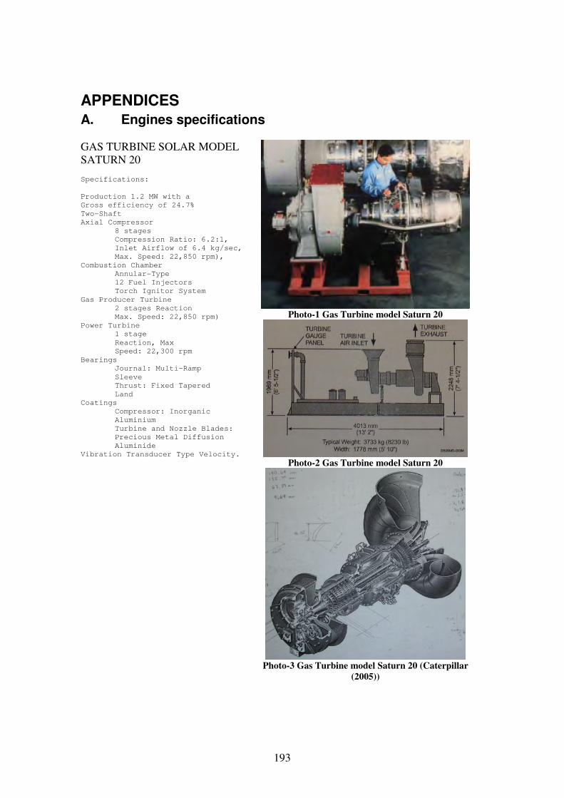
193
APPENDICES
A. Engines specifications GAS TURBINE SOLAR MODEL SATURN 20
Specifications:
Production 1.2 MW with a
Gross efficiency of 24.7%
Two-Shaft
Axial Compressor
8 stages
Compression Ratio: 6.2:1,
Inlet Airflow of 6.4 kg/sec,
Max. Speed: 22,850 rpm),
Combustion Chamber
Annular-Type
12 Fuel Injectors
Torch Ignitor System
Gas Producer Turbine
2 stages Reaction
Max. Speed: 22,850 rpm)
Power Turbine
1 stage
Reaction, Max
Speed: 22,300 rpm
Bearings
Journal: Multi-Ramp
Sleeve
Thrust: Fixed Tapered
Land
Coatings
Compressor: Inorganic
Aluminium
Turbine and Nozzle Blades:
Precious Metal Diffusion
Aluminide
Vibration Transducer Type Velocity.
Photo-1 Gas Turbine model Saturn 20
Photo-2 Gas Turbine model Saturn 20
Photo-3 Gas Turbine model Saturn 20 (Caterpillar
(2005))
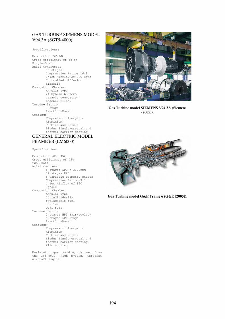
194
GAS TURBINE SIEMENS MODEL V94.3A (SGT5-4000) Specifications:
Production 260 MW
Gross efficiency of 38.5%
Single-Shaft
Axial Compressor
15 stages
Compression Ratio: 16:1
Inlet Airflow of 630 kg/s
Controlled diffusion
airfoils
Combustion Chamber
Annular-Type
24 hybrid burners
Ceramic combustion
chamber tiles)
Turbine Section
1 stage
Reaction-Power
Coatings
Compressor: Inorganic
Aluminium
Turbine and Nozzle
Blades Single-crystal and
thermal barrier coating
Gas Turbine model SIEMENS V94.3A (Siemens
(2005)).
GENERAL ELECTRIC MODEL FRAME 6B (LM6000)
Specifications:
Production 42.3 MW
Gross efficiency of 42%
Two-Shaft
Axial Compressor
5 stages LPC @ 3600rpm
14 stages HPC
6 variable geometry stages
Compression Ratio 29:1
Inlet Airflow of 120
kg/sec
Combustion Chamber
Annular-Type
30 individually
replaceable fuel
nozzles
Dual fuel
Turbine Section
2 stages HPT (air-cooled)
5 stages LPT Stage
Reaction-Power
Coatings
Compressor: Inorganic
Aluminium
Turbine and Nozzle
Blades Single-crystal and
thermal barrier coating
film cooling
Dual-rotor gas turbine, derived from
the CF6-80C2, high bypass, turbofan
aircraft engine.
Gas Turbine model G&E Frame 6 (G&E (2005)).
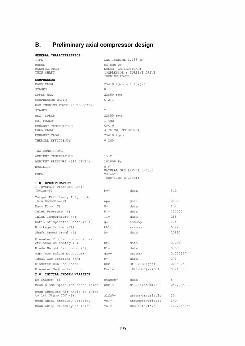
195
B. Preliminary axial compressor design GENERAL CHARACTERISTICS
TYPE GAS TURBINE 1.185 mw
MODEL SATURN 20
MANUFACTURER SOLAR (CATERPILLAR)
TWIN SHAFT COMPRESSOR & TURBINE DRIVE
TURBINE POWER
COMPRESSOR
MASS FLOW 23410 kg/h = 6.4 kg/s
STAGES 8
SPPED MAX 22850 rpm
COMPRESSOR RATIO 6.2:1
GAS TURBINE POWER (FULL LOAD)
STAGES 2
MAX. SPEED 22850 rpm
OUT POWER 1.4MW
EXHAUST TEMPERATURE 525 C
FUEL FLOW 4.75 MW (MM BTU/h)
EXHAUST FLOW 23410 kg/h
THERMAL EFFICIENCY 0.245
ISA CONDITIONS
AMBIENT TEMPERATURE 15 C
AMBIENT PRESSURE (SEA LEVEL) 101000 Pa
HUMIDITY 0.6
FUEL
NATURAL GAS LHV=31.5~43.3
MJ/nm^3
(800~1100 BTU/scf)
1.0. SPECIFICATION
1. Overall Pressure Ratio
(Solar=S) Rc= data 6.2
Target Efficiency Polytropic
(Ken Ramsden=KR) np= goal 0.88
Mass Flow (S) W= data 6.4
Inlet Pressure (S) P1= data 101000
Inlet Temperature (S) T1= data 288
Ratio of Specific Heats (KR) g= assump 1.4
Blockage factor (KR) kb1= assump 0.99
Shaft Speed [rpm] (S) N= data 22850
Diameter Tip 1st rotor, it is
cte=annulus config (S) Dt= data 0.281
Blade Height 1st rotor (S) B1= data 0.07
Gap (www.sulzermetco.com) gap= assump 0.000127
Ideal Gas Constant (KR) R= data 273
Diameter Hub 1st rotor Dhr1= Dt1-2(B1+gap) 0.140746
Diameter Medium 1st rotor Dmr1= (Dt1-Dh1)/2+Dh1 0.210873
2.0. INITIAL CHOSEN VARIABLE
No.Stages (S) stages= data 8
Mean Blade Speed 1st rotor inlet Umr1= N*3.1415*Dm1/60 252.285909
Mean Absolute Air Angle at Inlet
to 1st Stage IGV (S) alfa0= assumpt&variable 30
Mean Axial absoluty Velocity Vo1= assumpt&variable 140
Mean Axial Velocity at Inlet Va1= cos(alfa0)*Vo 121.246256
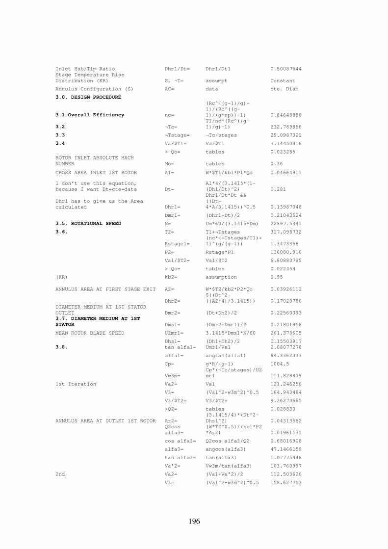
196
Inlet Hub/Tip Ratio Dhr1/Dt= Dhr1/Dt1 0.50087544
Stage Temperature Rise
Distribution (KR) S, ¬T= assumpt Constant
Annulus Configuration (S) AC= data cte. Diam
3.0. DESIGN PROCEDURE
3.1 Overall Efficiency nc=
(Rc^((g-1)/g)-
1)/(Rc^((g-
1)/(g*np))-1) 0.84648888
3.2 ¬Tc=
T1/nc*(Rc^((g-
1)/g)-1) 232.789856
3.3 ¬Tstage= ¬Tc/stages 29.0987321
3.4 Va/$T1= Va/$T1 7.14450416
> Qo= tables 0.023285
ROTOR INLET ABSOLUTE MACH
NUMBER Mo= tables 0.36
CROSS AREA INLET 1ST ROTOR A1= W*$T1/kb1*P1*Qo 0.04664911
I don’t use this equation,
because I want Dt=cte=data Dt=
A1*4/(3.1415*(1-
(Dh1/Dt)^2) 0.281
Dhr1 has to give us the Area
calculated Dhr1=
Dhr1/Dt*Dt &&
((Dt-
4*A/3.1415))^0.5 0.13987048
Dmr1= (Dhr1+Dt)/2 0.21043524
3.5. ROTATIONAL SPEED N= Um*60/(3.1415*Dm) 22897.5341
3.6. T2= T1+¬Tstages 317.098732
Rstage1=
(nc*(¬Tstages/T1)+
1)^(g/(g-1)) 1.3473358
P2= Rstage*P1 136080.916
Va1/$T2= Va1/$T2 6.80880795
> Qo= tables 0.022454
(KR) kb2= assumption 0.95
ANNULUS AREA AT FIRST STAGE EXIT A2= W*$T2/kb2*P2*Qo 0.03926112
Dhr2=
$((Dt^2-
((A2*4)/3.1415)) 0.17020786
DIAMETER MEDIUM AT 1ST STATOR
OUTLET Dmr2= (Dt+Dh2)/2 0.22560393
3.7. DIAMETER MEDIUM AT 1ST
STATOR Dms1= (Dmr2+Dmr1)/2 0.21801958
MEAN ROTOR BLADE SPEED U2mr1= 3.1415*Dms1*N/60 261.378605
Dhs1= (Dh1+Dh2)/2 0.15503917
3.8. tan alfa1= Umr1/Va1 2.08077278
alfa1= angtan(alfa1) 64.3362333
Cp= g*R/(g-1) 1004.5
Vw3m=
Cp*(¬Tc/stages)/U2
mr1 111.828879
1st Iteration Va2= Va1 121.246256
V3= (Va1^2+w3m^2)^0.5 164.943484
V3/$T2= V3/$T2= 9.26270665
>Q2= tables 0.028833
ANNULUS AREA AT OUTLET 1ST ROTOR Ar2=
(3.1415/4)*(Dt^2-
Dhs1^2) 0.04313582
Q2cos
alfa3=
(W*T2^0.5)/(kb1*P2
*Ar2) 0.01961131
cos alfa3= Q2cos alfa3/Q2 0.68016908
alfa3= angcos(alfa3) 47.1466159
tan alfa3= tan(alfa3) 1.07775448
Va'2= Vw3m/tan(alfa3) 103.760997
2nd Va2= (Va1+Va'2)/2 112.503626
V3= (Va1^2+w3m^2)^0.5 158.627753
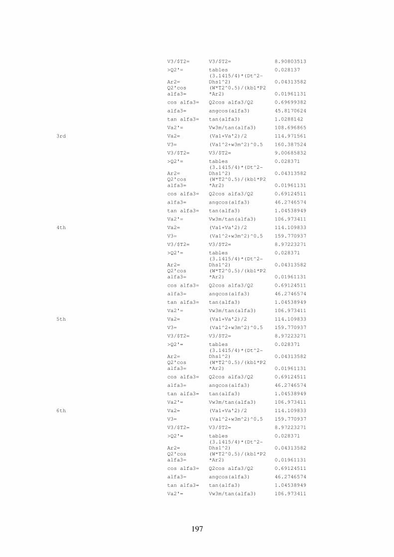
197
V3/$T2= V3/$T2= 8.90803513
>Q2'= tables 0.028137
Ar2=
(3.1415/4)*(Dt^2-
Dhs1^2) 0.04313582
Q2'cos
alfa3=
(W*T2^0.5)/(kb1*P2
*Ar2) 0.01961131
cos alfa3= Q2cos alfa3/Q2 0.69699382
alfa3= angcos(alfa3) 45.8170624
tan alfa3= tan(alfa3) 1.0288142
Va2'= Vw3m/tan(alfa3) 108.696865
3rd Va2= (Va1+Va'2)/2 114.971561
V3= (Va1^2+w3m^2)^0.5 160.387524
V3/$T2= V3/$T2= 9.00685832
>Q2'= tables 0.028371
Ar2=
(3.1415/4)*(Dt^2-
Dhs1^2) 0.04313582
Q2'cos
alfa3=
(W*T2^0.5)/(kb1*P2
*Ar2) 0.01961131
cos alfa3= Q2cos alfa3/Q2 0.69124511
alfa3= angcos(alfa3) 46.2746574
tan alfa3= tan(alfa3) 1.04538949
Va2'= Vw3m/tan(alfa3) 106.973411
4th Va2= (Va1+Va'2)/2 114.109833
V3= (Va1^2+w3m^2)^0.5 159.770937
V3/$T2= V3/$T2= 8.97223271
>Q2'= tables 0.028371
Ar2=
(3.1415/4)*(Dt^2-
Dhs1^2) 0.04313582
Q2'cos
alfa3=
(W*T2^0.5)/(kb1*P2
*Ar2) 0.01961131
cos alfa3= Q2cos alfa3/Q2 0.69124511
alfa3= angcos(alfa3) 46.2746574
tan alfa3= tan(alfa3) 1.04538949
Va2'= Vw3m/tan(alfa3) 106.973411
5th Va2= (Va1+Va'2)/2 114.109833
V3= (Va1^2+w3m^2)^0.5 159.770937
V3/$T2= V3/$T2= 8.97223271
>Q2'= tables 0.028371
Ar2=
(3.1415/4)*(Dt^2-
Dhs1^2) 0.04313582
Q2'cos
alfa3=
(W*T2^0.5)/(kb1*P2
*Ar2) 0.01961131
cos alfa3= Q2cos alfa3/Q2 0.69124511
alfa3= angcos(alfa3) 46.2746574
tan alfa3= tan(alfa3) 1.04538949
Va2'= Vw3m/tan(alfa3) 106.973411
6th Va2= (Va1+Va'2)/2 114.109833
V3= (Va1^2+w3m^2)^0.5 159.770937
V3/$T2= V3/$T2= 8.97223271
>Q2'= tables 0.028371
Ar2=
(3.1415/4)*(Dt^2-
Dhs1^2) 0.04313582
Q2'cos
alfa3=
(W*T2^0.5)/(kb1*P2
*Ar2) 0.01961131
cos alfa3= Q2cos alfa3/Q2 0.69124511
alfa3= angcos(alfa3) 46.2746574
tan alfa3= tan(alfa3) 1.04538949
Va2'= Vw3m/tan(alfa3) 106.973411
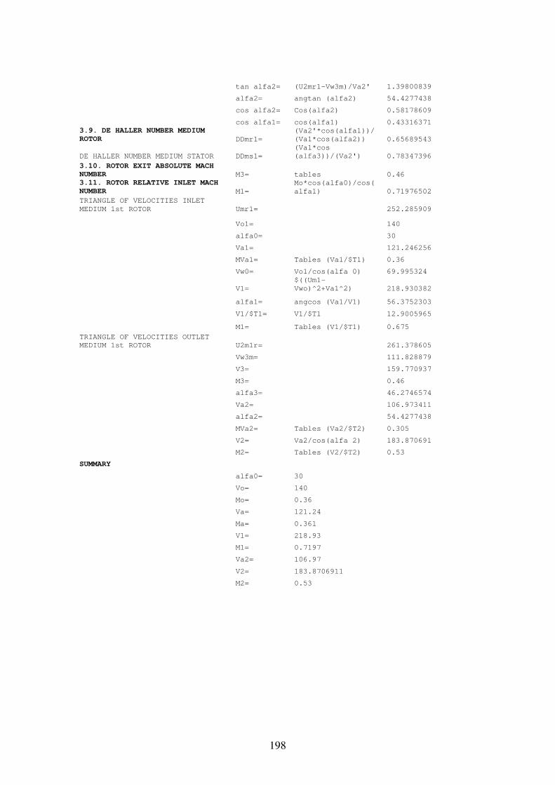
198
tan alfa2= (U2mr1-Vw3m)/Va2' 1.39800839
alfa2= angtan (alfa2) 54.4277438
cos alfa2= Cos(alfa2) 0.58178609
cos alfa1= cos(alfa1) 0.43316371
3.9. DE HALLER NUMBER MEDIUM
ROTOR DDmr1=
(Va2'*cos(alfa1))/
(Va1*cos(alfa2)) 0.65689543
DE HALLER NUMBER MEDIUM STATOR DDms1=
(Va1*cos
(alfa3))/(Va2') 0.78347396
3.10. ROTOR EXIT ABSOLUTE MACH
NUMBER M3= tables 0.46
3.11. ROTOR RELATIVE INLET MACH
NUMBER M1=
Mo*cos(alfa0)/cos(
alfa1) 0.71976502
TRIANGLE OF VELOCITIES INLET
MEDIUM 1st ROTOR Umr1= 252.285909
Vo1= 140
alfa0= 30
Va1= 121.246256
MVa1= Tables (Va1/$T1) 0.36
Vw0= Vo1/cos(alfa 0) 69.995324
V1=
$((Um1-
Vwo)^2+Va1^2) 218.930382
alfa1= angcos (Va1/V1) 56.3752303
V1/$T1= V1/$T1 12.9005965
M1= Tables (V1/$T1) 0.675
TRIANGLE OF VELOCITIES OUTLET
MEDIUM 1st ROTOR U2m1r= 261.378605
Vw3m= 111.828879
V3= 159.770937
M3= 0.46
alfa3= 46.2746574
Va2= 106.973411
alfa2= 54.4277438
MVa2= Tables (Va2/$T2) 0.305
V2= Va2/cos(alfa 2) 183.870691
M2= Tables (V2/$T2) 0.53
SUMMARY
alfa0= 30
Vo= 140
Mo= 0.36
Va= 121.24
Ma= 0.361
V1= 218.93
M1= 0.7197
Va2= 106.97
V2= 183.8706911
M2= 0.53
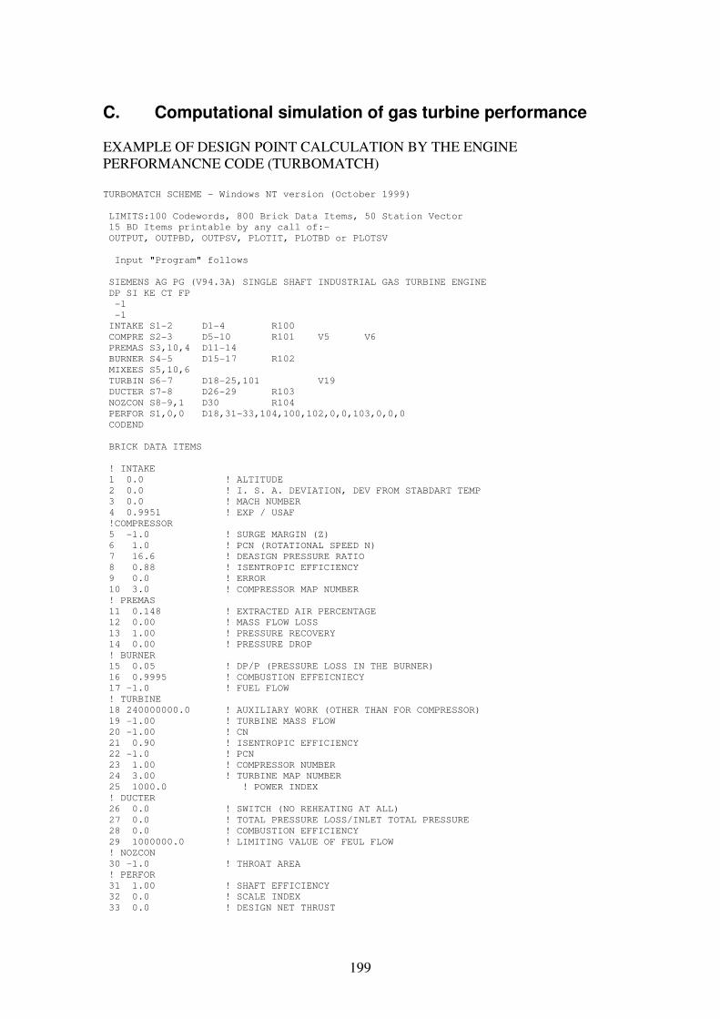
199
C. Computational simulation of gas turbine performance EXAMPLE OF DESIGN POINT CALCULATION BY THE ENGINE PERFORMANCNE CODE (TURBOMATCH) TURBOMATCH SCHEME - Windows NT version (October 1999)
LIMITS:100 Codewords, 800 Brick Data Items, 50 Station Vector
15 BD Items printable by any call of:-
OUTPUT, OUTPBD, OUTPSV, PLOTIT, PLOTBD or PLOTSV
Input "Program" follows
SIEMENS AG PG (V94.3A) SINGLE SHAFT INDUSTRIAL GAS TURBINE ENGINE
DP SI KE CT FP
-1
-1
INTAKE S1-2 D1-4 R100
COMPRE S2-3 D5-10 R101 V5 V6
PREMAS S3,10,4 D11-14
BURNER S4-5 D15-17 R102
MIXEES S5,10,6
TURBIN S6-7 D18-25,101 V19
DUCTER S7-8 D26-29 R103
NOZCON S8-9,1 D30 R104
PERFOR S1,0,0 D18,31-33,104,100,102,0,0,103,0,0,0
CODEND
BRICK DATA ITEMS
! INTAKE
1 0.0 ! ALTITUDE
2 0.0 ! I. S. A. DEVIATION, DEV FROM STABDART TEMP
3 0.0 ! MACH NUMBER
4 0.9951 ! EXP / USAF
!COMPRESSOR
5 -1.0 ! SURGE MARGIN (Z)
6 1.0 ! PCN (ROTATIONAL SPEED N)
7 16.6 ! DEASIGN PRESSURE RATIO
8 0.88 ! ISENTROPIC EFFICIENCY
9 0.0 ! ERROR
10 3.0 ! COMPRESSOR MAP NUMBER
! PREMAS
11 0.148 ! EXTRACTED AIR PERCENTAGE
12 0.00 ! MASS FLOW LOSS
13 1.00 ! PRESSURE RECOVERY
14 0.00 ! PRESSURE DROP
! BURNER
15 0.05 ! DP/P (PRESSURE LOSS IN THE BURNER)
16 0.9995 ! COMBUSTION EFFEICNIECY
17 -1.0 ! FUEL FLOW
! TURBINE
18 240000000.0 ! AUXILIARY WORK (OTHER THAN FOR COMPRESSOR)
19 -1.00 ! TURBINE MASS FLOW
20 -1.00 ! CN
21 0.90 ! ISENTROPIC EFFICIENCY
22 -1.0 ! PCN
23 1.00 ! COMPRESSOR NUMBER
24 3.00 ! TURBINE MAP NUMBER
25 1000.0 ! POWER INDEX
! DUCTER
26 0.0 ! SWITCH (NO REHEATING AT ALL)
27 0.0 ! TOTAL PRESSURE LOSS/INLET TOTAL PRESSURE
28 0.0 ! COMBUSTION EFFICIENCY
29 1000000.0 ! LIMITING VALUE OF FEUL FLOW
! NOZCON
30 -1.0 ! THROAT AREA
! PERFOR
31 1.00 ! SHAFT EFFICIENCY
32 0.0 ! SCALE INDEX
33 0.0 ! DESIGN NET THRUST
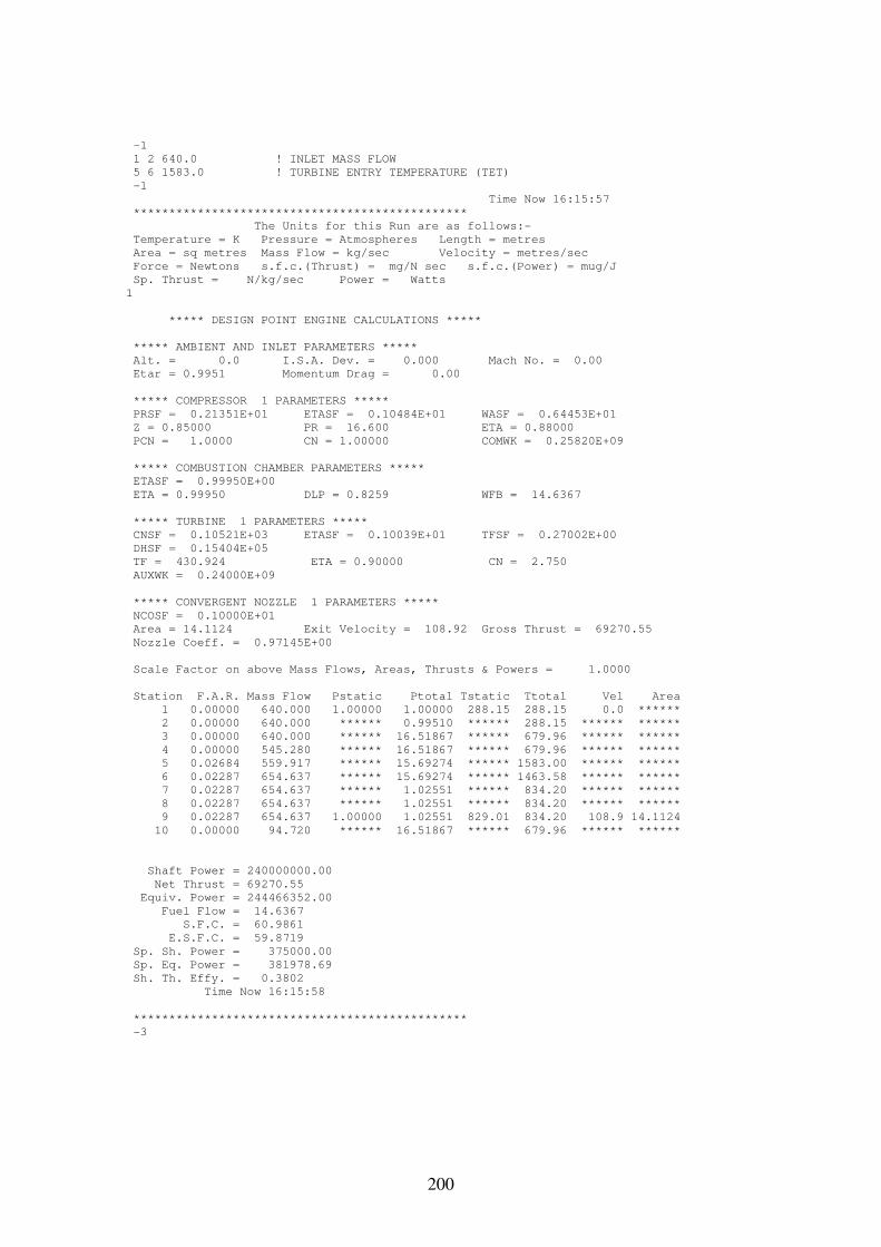
200
-1
1 2 640.0 ! INLET MASS FLOW
5 6 1583.0 ! TURBINE ENTRY TEMPERATURE (TET)
-1
Time Now 16:15:57
***********************************************
The Units for this Run are as follows:-
Temperature = K Pressure = Atmospheres Length = metres
Area = sq metres Mass Flow = kg/sec Velocity = metres/sec
Force = Newtons s.f.c.(Thrust) = mg/N sec s.f.c.(Power) = mug/J
Sp. Thrust = N/kg/sec Power = Watts
1
***** DESIGN POINT ENGINE CALCULATIONS *****
***** AMBIENT AND INLET PARAMETERS *****
Alt. = 0.0 I.S.A. Dev. = 0.000 Mach No. = 0.00
Etar = 0.9951 Momentum Drag = 0.00
***** COMPRESSOR 1 PARAMETERS *****
PRSF = 0.21351E+01 ETASF = 0.10484E+01 WASF = 0.64453E+01
Z = 0.85000 PR = 16.600 ETA = 0.88000
PCN = 1.0000 CN = 1.00000 COMWK = 0.25820E+09
***** COMBUSTION CHAMBER PARAMETERS *****
ETASF = 0.99950E+00
ETA = 0.99950 DLP = 0.8259 WFB = 14.6367
***** TURBINE 1 PARAMETERS *****
CNSF = 0.10521E+03 ETASF = 0.10039E+01 TFSF = 0.27002E+00
DHSF = 0.15404E+05
TF = 430.924 ETA = 0.90000 CN = 2.750
AUXWK = 0.24000E+09
***** CONVERGENT NOZZLE 1 PARAMETERS *****
NCOSF = 0.10000E+01
Area = 14.1124 Exit Velocity = 108.92 Gross Thrust = 69270.55
Nozzle Coeff. = 0.97145E+00
Scale Factor on above Mass Flows, Areas, Thrusts & Powers = 1.0000
Station F.A.R. Mass Flow Pstatic Ptotal Tstatic Ttotal Vel Area
1 0.00000 640.000 1.00000 1.00000 288.15 288.15 0.0 ******
2 0.00000 640.000 ****** 0.99510 ****** 288.15 ****** ******
3 0.00000 640.000 ****** 16.51867 ****** 679.96 ****** ******
4 0.00000 545.280 ****** 16.51867 ****** 679.96 ****** ******
5 0.02684 559.917 ****** 15.69274 ****** 1583.00 ****** ******
6 0.02287 654.637 ****** 15.69274 ****** 1463.58 ****** ******
7 0.02287 654.637 ****** 1.02551 ****** 834.20 ****** ******
8 0.02287 654.637 ****** 1.02551 ****** 834.20 ****** ******
9 0.02287 654.637 1.00000 1.02551 829.01 834.20 108.9 14.1124
10 0.00000 94.720 ****** 16.51867 ****** 679.96 ****** ******
Shaft Power = 240000000.00
Net Thrust = 69270.55
Equiv. Power = 244466352.00
Fuel Flow = 14.6367
S.F.C. = 60.9861
E.S.F.C. = 59.8719
Sp. Sh. Power = 375000.00
Sp. Eq. Power = 381978.69
Sh. Th. Effy. = 0.3802
Time Now 16:15:58
***********************************************
-3
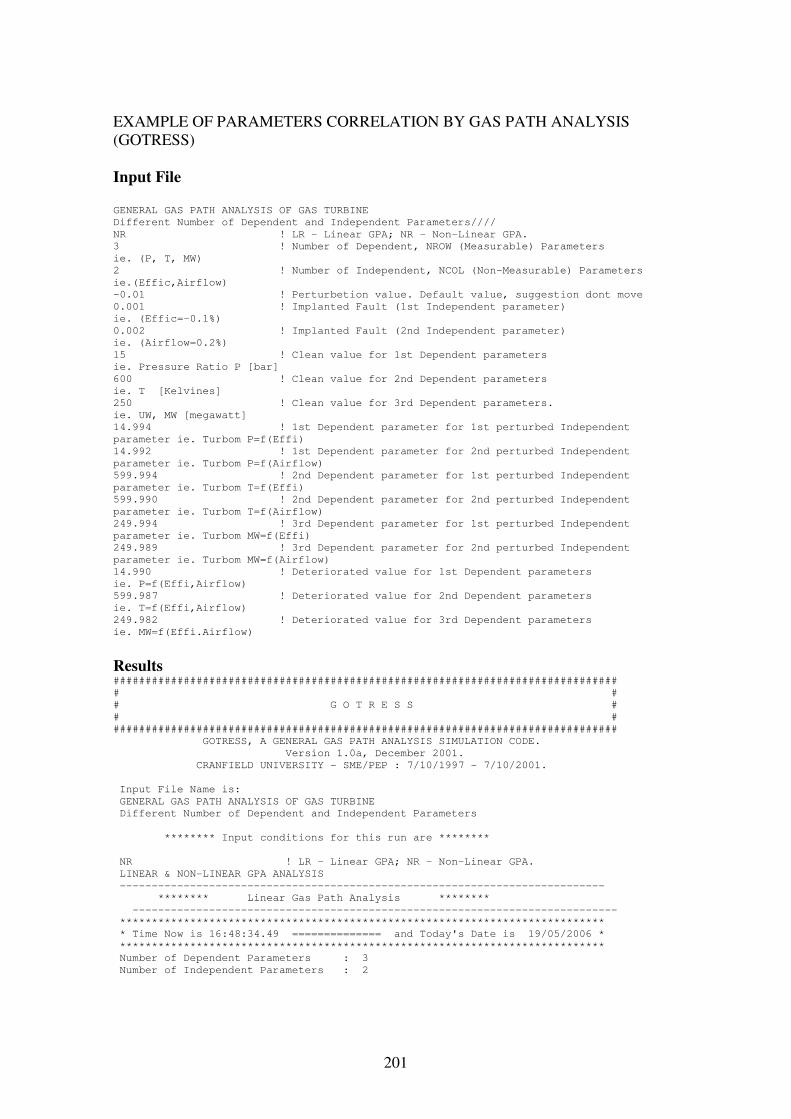
201
EXAMPLE OF PARAMETERS CORRELATION BY GAS PATH ANALYSIS (GOTRESS) Input File
GENERAL GAS PATH ANALYSIS OF GAS TURBINE
Different Number of Dependent and Independent Parameters////
NR ! LR - Linear GPA; NR - Non-Linear GPA.
3 ! Number of Dependent, NROW (Measurable) Parameters
ie. (P, T, MW)
2 ! Number of Independent, NCOL (Non-Measurable) Parameters
ie.(Effic,Airflow)
-0.01 ! Perturbetion value. Default value, suggestion dont move
0.001 ! Implanted Fault (1st Independent parameter)
ie. (Effic=-0.1%)
0.002 ! Implanted Fault (2nd Independent parameter)
ie. (Airflow=0.2%)
15 ! Clean value for 1st Dependent parameters
ie. Pressure Ratio P [bar]
600 ! Clean value for 2nd Dependent parameters
ie. T [Kelvines]
250 ! Clean value for 3rd Dependent parameters.
ie. UW, MW [megawatt]
14.994 ! 1st Dependent parameter for 1st perturbed Independent
parameter ie. Turbom P=f(Effi)
14.992 ! 1st Dependent parameter for 2nd perturbed Independent
parameter ie. Turbom P=f(Airflow)
599.994 ! 2nd Dependent parameter for 1st perturbed Independent
parameter ie. Turbom T=f(Effi)
599.990 ! 2nd Dependent parameter for 2nd perturbed Independent
parameter ie. Turbom T=f(Airflow)
249.994 ! 3rd Dependent parameter for 1st perturbed Independent
parameter ie. Turbom MW=f(Effi)
249.989 ! 3rd Dependent parameter for 2nd perturbed Independent
parameter ie. Turbom MW=f(Airflow)
14.990 ! Deteriorated value for 1st Dependent parameters
ie. P=f(Effi,Airflow)
599.987 ! Deteriorated value for 2nd Dependent parameters
ie. T=f(Effi,Airflow)
249.982 ! Deteriorated value for 3rd Dependent parameters
ie. MW=f(Effi.Airflow)
Results ###############################################################################
# #
# G O T R E S S #
# #
###############################################################################
GOTRESS, A GENERAL GAS PATH ANALYSIS SIMULATION CODE.
Version 1.0a, December 2001.
CRANFIELD UNIVERSITY - SME/PEP : 7/10/1997 - 7/10/2001.
Input File Name is:
GENERAL GAS PATH ANALYSIS OF GAS TURBINE
Different Number of Dependent and Independent Parameters
******** Input conditions for this run are ********
NR ! LR - Linear GPA; NR - Non-Linear GPA.
LINEAR & NON-LINEAR GPA ANALYSIS
----------------------------------------------------------------------------
******** Linear Gas Path Analysis ********
----------------------------------------------------------------------------
****************************************************************************
* Time Now is 16:48:34.49 ============== and Today's Date is 19/05/2006 *
****************************************************************************
Number of Dependent Parameters : 3
Number of Independent Parameters : 2
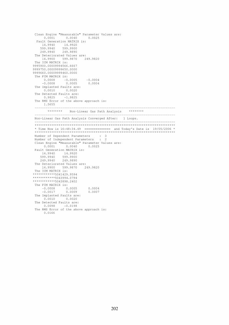
202
Clean Engine "Measurable" Parameter Values are:
0.0001 0.0040 0.0025
Fault Generation MATRIX is:
14.9940 14.9920
599.9940 599.9900
249.9940 249.9890
The Deteriorated Values are:
14.9900 599.9870 249.9820
The ICM MATRIX is:
9995900.00009994566.6667
9999750.00009999650.0000
9999660.00009999460.0000
The FCM MATRIX is:
0.0008 -0.0005 -0.0004
-0.0008 0.0005 0.0004
The Implanted Faults are:
0.0010 0.0020
The Detected Faults are:
0.9825 -1.9825
The RMS Error of the above approach is:
1.5655
----------------------------------------------------------------------------
******** Non-Linear Gas Path Analysis ********
----------------------------------------------------------------------------
Non-Linear Gas Path Analysis Converged After: 1 Loops.
----------------------------------------------------------------------------
****************************************************************************
* Time Now is 16:48:34.49 ============== and Today's Date is 19/05/2006 *
****************************************************************************
Number of Dependent Parameters : 3
Number of Independent Parameters : 2
Clean Engine "Measurable" Parameter Values are:
0.0001 0.0040 0.0025
Fault Generation MATRIX is:
14.9940 14.9920
599.9940 599.9900
249.9940 249.9890
The Deteriorated Values are:
14.9900 599.9870 249.9820
The ICM MATRIX is:
************5041429.9594
************5043994.0794
************5043898.2402
The FCM MATRIX is:
-0.0008 0.0005 0.0004
-0.0017 0.0009 0.0007
The Implanted Faults are:
0.0010 0.0020
The Detected Faults are:
0.0098 -0.0198
The RMS Error of the above approach is:
0.0166
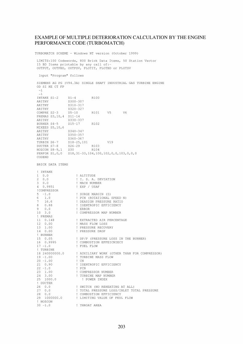
203
EXAMPLE OF MULTIPLE DETERIORATION CALCULATION BY THE ENGINE PERFORMANCE CODE (TURBOMATCH) TURBOMATCH SCHEME - Windows NT version (October 1999)
LIMITS:100 Codewords, 800 Brick Data Items, 50 Station Vector
15 BD Items printable by any call of:-
OUTPUT, OUTPBD, OUTPSV, PLOTIT, PLOTBD or PLOTSV
Input "Program" follows
SIEMENS AG PG (V94.3A) SINGLE SHAFT INDUSTRIAL GAS TURBINE ENGINE
OD SI KE CT FP
-1
-1
INTAKE S1-2 D1-4 R100
ARITHY D300-307
ARITHY D310-317
ARITHY D320-327
COMPRE S2-3 D5-10 R101 V5 V6
PREMAS S3,10,4 D11-14
ARITHY D330-337
BURNER S4-5 D15-17 R102
MIXEES S5,10,6
ARITHY D340-347
ARITHY D350-357
ARITHY D360-367
TURBIN S6-7 D18-25,101 V19
DUCTER S7-8 D26-29 R103
NOZCON S8-9,1 D30 R104
PERFOR S1,0,0 D18,31-33,104,100,102,0,0,103,0,0,0
CODEND
BRICK DATA ITEMS
! INTAKE
1 0.0 ! ALTITUDE
2 0.0 ! I. S. A. DEVIATION
3 0.0 ! MACH NUMBER
4 0.9951 ! EXP / USAF
!COMPRESSOR
5 -1.0 ! SURGE MARGIN (Z)
6 1.0 ! PCN (ROTATIONAL SPEED N)
7 16.6 ! DEASIGN PRESSURE RATIO
8 0.88 ! ISENTROPIC EFFICIENCY
9 0.0 ! ERROR
10 3.0 ! COMPRESSOR MAP NUMBER
! PREMAS
11 0.148 ! EXTRACTED AIR PERCENTAGE
12 0.00 ! MASS FLOW LOSS
13 1.00 ! PRESSURE RECOVERY
14 0.00 ! PRESSURE DROP
! BURNER
15 0.05 ! DP/P (PRESSURE LOSS IN THE BURNER)
16 0.9995 ! COMBUSTION EFFEICNIECY
17 -1.0 ! FUEL FLOW
! TURBINE
18 240000000.0 ! AUXILIARY WORK (OTHER THAN FOR COMPRESSOR)
19 -1.00 ! TURBINE MASS FLOW
20 -1.00 ! CN
21 0.90 ! ISENTROPIC EFFICIENCY
22 -1.0 ! PCN
23 1.00 ! COMPRESSOR NUMBER
24 3.00 ! TURBINE MAP NUMBER
25 1000.0 ! POWER INDEX
! DUCTER
26 0.0 ! SWITCH (NO REHEATING AT ALL)
27 0.0 ! TOTAL PRESSURE LOSS/INLET TOTAL PRESSURE
28 0.0 ! COMBUSTION EFFICIENCY
29 1000000.0 ! LIMITING VALUE OF FEUL FLOW
! NOZCON
30 -1.0 ! THROAT AREA
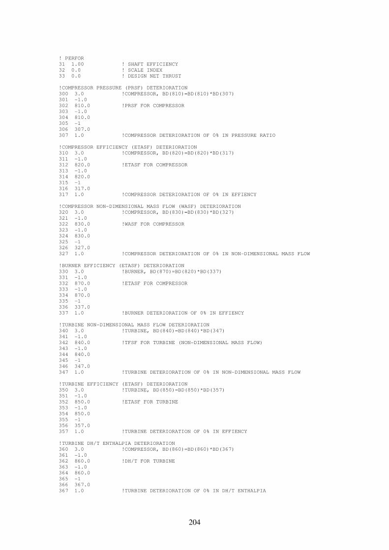
204
! PERFOR
31 1.00 ! SHAFT EFFICIENCY
32 0.0 ! SCALE INDEX
33 0.0 ! DESIGN NET THRUST
!COMPRESSOR PRESSURE (PRSF) DETERIORATION
300 3.0 !COMPRESSOR, BD(810)=BD(810)*BD(307)
301 -1.0
302 810.0 !PRSF FOR COMPRESSOR
303 -1.0
304 810.0
305 -1
306 307.0
307 1.0 !COMPRESSOR DETERIORATION OF 0% IN PRESSURE RATIO
!COMPRESSOR EFFICIENCY (ETASF) DETERIORATION
310 3.0 !COMPRESSOR, BD(820)=BD(820)*BD(317)
311 -1.0
312 820.0 !ETASF FOR COMPRESSOR
313 -1.0
314 820.0
315 -1
316 317.0
317 1.0 !COMPRESSOR DETERIORATION OF 0% IN EFFIENCY
!COMPRESSOR NON-DIMENSIONAL MASS FLOW (WASF) DETERIORATION
320 3.0 !COMPRESSOR, BD(830)=BD(830)*BD(327)
321 -1.0
322 830.0 !WASF FOR COMPRESSOR
323 -1.0
324 830.0
325 -1
326 327.0
327 1.0 !COMPRESSOR DETERIORATION OF 0% IN NON-DIMENSIONAL MASS FLOW
!BURNER EFFICIENCY (ETASF) DETERIORATION
330 3.0 !BURNER, BD(870)=BD(820)*BD(337)
331 -1.0
332 870.0 !ETASF FOR COMPRESSOR
333 -1.0
334 870.0
335 -1
336 337.0
337 1.0 !BURNER DETERIORATION OF 0% IN EFFIENCY
!TURBINE NON-DIMENSIONAL MASS FLOW DETERIORATION
340 3.0 !TURBINE, BD(840)=BD(840)*BD(347)
341 -1.0
342 840.0 !TFSF FOR TURBINE (NON-DIMENSIONAL MASS FLOW)
343 -1.0
344 840.0
345 -1
346 347.0
347 1.0 !TURBINE DETERIORATION OF 0% IN NON-DIMENSIONAL MASS FLOW
!TURBINE EFFICIENCY (ETASF) DETERIORATION
350 3.0 !TURBINE, BD(850)=BD(850)*BD(357)
351 -1.0
352 850.0 !ETASF FOR TURBINE
353 -1.0
354 850.0
355 -1
356 357.0
357 1.0 !TURBINE DETERIORATION OF 0% IN EFFIENCY
!TURBINE DH/T ENTHALPIA DETERIORATION
360 3.0 !COMPRESSOR, BD(860)=BD(860)*BD(367)
361 -1.0
362 860.0 !DH/T FOR TURBINE
363 -1.0
364 860.0
365 -1
366 367.0
367 1.0 !TURBINE DETERIORATION OF 0% IN DH/T ENTHALPIA
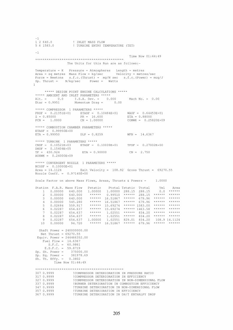
205
-1
1 2 640.0 ! INLET MASS FLOW
5 6 1583.0 ! TURBINE ENTRY TEMPERATURE (TET)
-1
Time Now 01:44:49
***********************************************
The Units for this Run are as follows:-
Temperature = K Pressure = Atmospheres Length = metres
Area = sq metres Mass Flow = kg/sec Velocity = metres/sec
Force = Newtons s.f.c.(Thrust) = mg/N sec s.f.c.(Power) = mug/J
Sp. Thrust = N/kg/sec Power = Watts
1
***** DESIGN POINT ENGINE CALCULATIONS *****
***** AMBIENT AND INLET PARAMETERS *****
Alt. = 0.0 I.S.A. Dev. = 0.000 Mach No. = 0.00
Etar = 0.9951 Momentum Drag = 0.00
***** COMPRESSOR 1 PARAMETERS *****
PRSF = 0.21351E+01 ETASF = 0.10484E+01 WASF = 0.64453E+01
Z = 0.85000 PR = 16.600 ETA = 0.88000
PCN = 1.0000 CN = 1.00000 COMWK = 0.25820E+09
***** COMBUSTION CHAMBER PARAMETERS *****
ETASF = 0.99950E+00
ETA = 0.99950 DLP = 0.8259 WFB = 14.6367
***** TURBINE 1 PARAMETERS *****
CNSF = 0.10521E+03 ETASF = 0.10039E+01 TFSF = 0.27002E+00
DHSF = 0.15404E+05
TF = 430.924 ETA = 0.90000 CN = 2.750
AUXWK = 0.24000E+09
***** CONVERGENT NOZZLE 1 PARAMETERS *****
NCOSF = 0.10000E+01
Area = 14.1124 Exit Velocity = 108.92 Gross Thrust = 69270.55
Nozzle Coeff. = 0.97145E+00
Scale Factor on above Mass Flows, Areas, Thrusts & Powers = 1.0000
Station F.A.R. Mass Flow Pstatic Ptotal Tstatic Ttotal Vel Area
1 0.00000 640.000 1.00000 1.00000 288.15 288.15 0.0 ******
2 0.00000 640.000 ****** 0.99510 ****** 288.15 ****** ******
3 0.00000 640.000 ****** 16.51867 ****** 679.96 ****** ******
4 0.00000 545.280 ****** 16.51867 ****** 679.96 ****** ******
5 0.02684 559.917 ****** 15.69274 ****** 1583.00 ****** ******
6 0.02287 654.637 ****** 15.69274 ****** 1463.58 ****** ******
7 0.02287 654.637 ****** 1.02551 ****** 834.20 ****** ******
8 0.02287 654.637 ****** 1.02551 ****** 834.20 ****** ******
9 0.02287 654.637 1.00000 1.02551 829.01 834.20 108.9 14.1124
10 0.00000 94.720 ****** 16.51867 ****** 679.96 ****** ******
Shaft Power = 240000000.00
Net Thrust = 69270.55
Equiv. Power = 244466352.00
Fuel Flow = 14.6367
S.F.C. = 60.9861
E.S.F.C. = 59.8719
Sp. Sh. Power = 375000.00
Sp. Eq. Power = 381978.69
Sh. Th. Effy. = 0.3802
Time Now 01:44:49
***********************************************
307 0.9999 !COMPRESSOR DETERIORATION IN PRESSURE RATIO
317 0.9999 !COMPRESSOR DETERIORATION IN EFFICIENCY
327 0.9999 !COMPRESSOR DETERIORATION IN NON-DIMENSIONAL FLOW
337 0.9999 !BURNER DETERIORATION IN COMBUSTION EFFICIENCY
347 0.9999 !TURBINE DETERIORATION IN NON-DIMENSIONAL FLOW
357 0.9999 !TURBINE DETERIORATION IN EFFICIENCY
367 0.9999 !TURBINE DETERIORATION IN DH/T ENTHALPY DROP
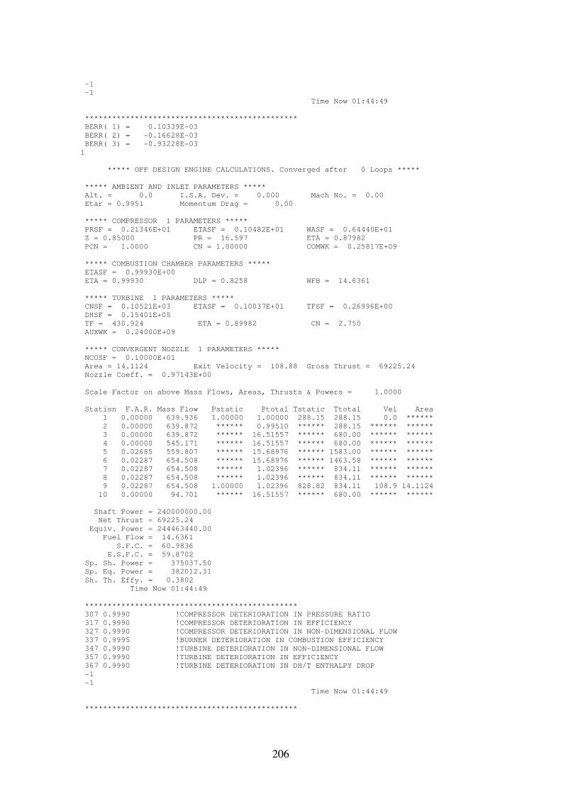
206
-1
-1
Time Now 01:44:49
***********************************************
BERR( 1) = 0.10339E-03
BERR( 2) = -0.16628E-03
BERR( 3) = -0.93228E-03
1
***** OFF DESIGN ENGINE CALCULATIONS. Converged after 0 Loops *****
***** AMBIENT AND INLET PARAMETERS *****
Alt. = 0.0 I.S.A. Dev. = 0.000 Mach No. = 0.00
Etar = 0.9951 Momentum Drag = 0.00
***** COMPRESSOR 1 PARAMETERS *****
PRSF = 0.21346E+01 ETASF = 0.10482E+01 WASF = 0.64440E+01
Z = 0.85000 PR = 16.597 ETA = 0.87982
PCN = 1.0000 CN = 1.00000 COMWK = 0.25817E+09
***** COMBUSTION CHAMBER PARAMETERS *****
ETASF = 0.99930E+00
ETA = 0.99930 DLP = 0.8258 WFB = 14.6361
***** TURBINE 1 PARAMETERS *****
CNSF = 0.10521E+03 ETASF = 0.10037E+01 TFSF = 0.26996E+00
DHSF = 0.15401E+05
TF = 430.924 ETA = 0.89982 CN = 2.750
AUXWK = 0.24000E+09
***** CONVERGENT NOZZLE 1 PARAMETERS *****
NCOSF = 0.10000E+01
Area = 14.1124 Exit Velocity = 108.88 Gross Thrust = 69225.24
Nozzle Coeff. = 0.97143E+00
Scale Factor on above Mass Flows, Areas, Thrusts & Powers = 1.0000
Station F.A.R. Mass Flow Pstatic Ptotal Tstatic Ttotal Vel Area
1 0.00000 639.936 1.00000 1.00000 288.15 288.15 0.0 ******
2 0.00000 639.872 ****** 0.99510 ****** 288.15 ****** ******
3 0.00000 639.872 ****** 16.51557 ****** 680.00 ****** ******
4 0.00000 545.171 ****** 16.51557 ****** 680.00 ****** ******
5 0.02685 559.807 ****** 15.68976 ****** 1583.00 ****** ******
6 0.02287 654.508 ****** 15.68976 ****** 1463.58 ****** ******
7 0.02287 654.508 ****** 1.02396 ****** 834.11 ****** ******
8 0.02287 654.508 ****** 1.02396 ****** 834.11 ****** ******
9 0.02287 654.508 1.00000 1.02396 828.82 834.11 108.9 14.1124
10 0.00000 94.701 ****** 16.51557 ****** 680.00 ****** ******
Shaft Power = 240000000.00
Net Thrust = 69225.24
Equiv. Power = 244463440.00
Fuel Flow = 14.6361
S.F.C. = 60.9836
E.S.F.C. = 59.8702
Sp. Sh. Power = 375037.50
Sp. Eq. Power = 382012.31
Sh. Th. Effy. = 0.3802
Time Now 01:44:49
***********************************************
307 0.9990 !COMPRESSOR DETERIORATION IN PRESSURE RATIO
317 0.9990 !COMPRESSOR DETERIORATION IN EFFICIENCY
327 0.9990 !COMPRESSOR DETERIORATION IN NON-DIMENSIONAL FLOW
337 0.9995 !BURNER DETERIORATION IN COMBUSTION EFFICIENCY
347 0.9990 !TURBINE DETERIORATION IN NON-DIMENSIONAL FLOW
357 0.9990 !TURBINE DETERIORATION IN EFFICIENCY
367 0.9990 !TURBINE DETERIORATION IN DH/T ENTHALPY DROP
-1
-1
Time Now 01:44:49
***********************************************
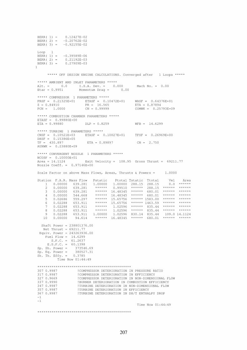
207
BERR( 1) = 0.12427E-02
BERR( 2) = -0.20762E-02
BERR( 3) = -0.92155E-02
Loop 1
BERR( 1) = -0.39589E-06
BERR( 2) = 0.21192E-03
BERR( 3) = 0.27909E-03
1
***** OFF DESIGN ENGINE CALCULATIONS. Converged after 1 Loops *****
***** AMBIENT AND INLET PARAMETERS *****
Alt. = 0.0 I.S.A. Dev. = 0.000 Mach No. = 0.00
Etar = 0.9951 Momentum Drag = 0.00
***** COMPRESSOR 1 PARAMETERS *****
PRSF = 0.21325E+01 ETASF = 0.10472E+01 WASF = 0.64376E+01
Z = 0.84910 PR = 16.565 ETA = 0.87894
PCN = 1.0000 CN = 0.99999 COMWK = 0.25793E+09
***** COMBUSTION CHAMBER PARAMETERS *****
ETASF = 0.99880E+00
ETA = 0.99880 DLP = 0.8259 WFB = 14.6299
***** TURBINE 1 PARAMETERS *****
CNSF = 0.10521E+03 ETASF = 0.10027E+01 TFSF = 0.26969E+00
DHSF = 0.15386E+05
TF = 430.897 ETA = 0.89897 CN = 2.750
AUXWK = 0.23880E+09
***** CONVERGENT NOZZLE 1 PARAMETERS *****
NCOSF = 0.10000E+01
Area = 14.1124 Exit Velocity = 108.95 Gross Thrust = 69211.77
Nozzle Coeff. = 0.97146E+00
Scale Factor on above Mass Flows, Areas, Thrusts & Powers = 1.0000
Station F.A.R. Mass Flow Pstatic Ptotal Tstatic Ttotal Vel Area
1 0.00000 639.281 1.00000 1.00000 288.15 288.15 0.0 ******
2 0.00000 639.281 ****** 0.99510 ****** 288.15 ****** ******
3 0.00000 639.281 ****** 16.48345 ****** 680.01 ****** ******
4 0.00000 544.668 ****** 16.48345 ****** 680.01 ****** ******
5 0.02686 559.297 ****** 15.65756 ****** 1583.00 ****** ******
6 0.02288 653.911 ****** 15.65756 ****** 1463.59 ****** ******
7 0.02288 653.911 ****** 1.02596 ****** 835.44 ****** ******
8 0.02288 653.911 ****** 1.02596 ****** 835.44 ****** ******
9 0.02288 653.911 1.00000 1.02596 830.14 835.44 109.0 14.1124
10 0.00000 94.614 ****** 16.48345 ****** 680.01 ****** ******
Shaft Power = 238801376.00
Net Thrust = 69211.77
Equiv. Power = 243263936.00
Fuel Flow = 14.6299
S.F.C. = 61.2637
E.S.F.C. = 60.1398
Sp. Sh. Power = 373546.69
Sp. Eq. Power = 380527.31
Sh. Th. Effy. = 0.3785
Time Now 01:44:49
***********************************************
307 0.9987 !COMPRESSOR DETERIORATION IN PRESSURE RATIO
317 0.9987 !COMPRESSOR DETERIORATION IN EFFICIENCY
327 0.9669 !COMPRESSOR DETERIORATION IN NON-DIMENSIONAL FLOW
337 0.9990 !BURNER DETERIORATION IN COMBUSTION EFFICIENCY
347 0.9987 !TURBINE DETERIORATION IN NON-DIMENSIONAL FLOW
357 0.9987 !TURBINE DETERIORATION IN EFFICIENCY
367 0.9987 !TURBINE DETERIORATION IN DH/T ENTHALPY DROP
-1
-1
Time Now 01:44:49
***********************************************
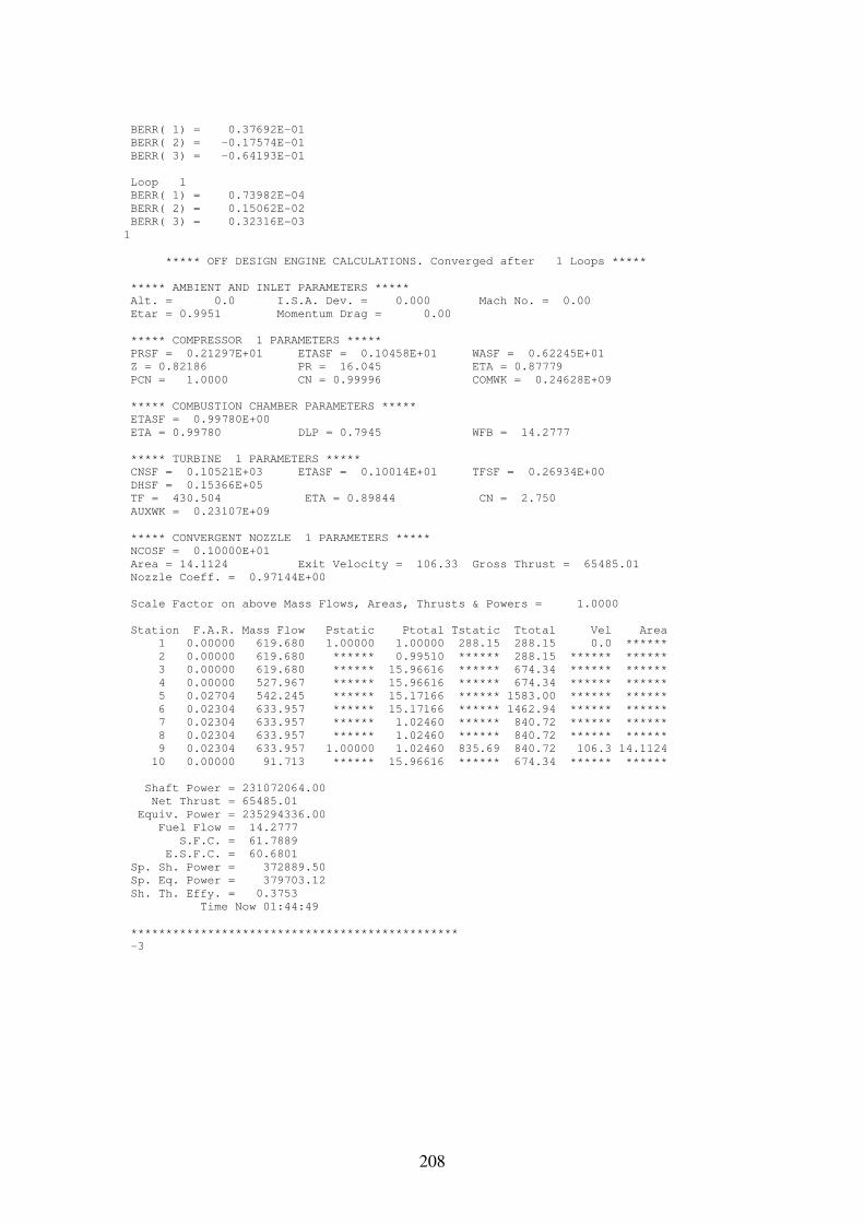
208
BERR( 1) = 0.37692E-01
BERR( 2) = -0.17574E-01
BERR( 3) = -0.64193E-01
Loop 1
BERR( 1) = 0.73982E-04
BERR( 2) = 0.15062E-02
BERR( 3) = 0.32316E-03
1
***** OFF DESIGN ENGINE CALCULATIONS. Converged after 1 Loops *****
***** AMBIENT AND INLET PARAMETERS *****
Alt. = 0.0 I.S.A. Dev. = 0.000 Mach No. = 0.00
Etar = 0.9951 Momentum Drag = 0.00
***** COMPRESSOR 1 PARAMETERS *****
PRSF = 0.21297E+01 ETASF = 0.10458E+01 WASF = 0.62245E+01
Z = 0.82186 PR = 16.045 ETA = 0.87779
PCN = 1.0000 CN = 0.99996 COMWK = 0.24628E+09
***** COMBUSTION CHAMBER PARAMETERS *****
ETASF = 0.99780E+00
ETA = 0.99780 DLP = 0.7945 WFB = 14.2777
***** TURBINE 1 PARAMETERS *****
CNSF = 0.10521E+03 ETASF = 0.10014E+01 TFSF = 0.26934E+00
DHSF = 0.15366E+05
TF = 430.504 ETA = 0.89844 CN = 2.750
AUXWK = 0.23107E+09
***** CONVERGENT NOZZLE 1 PARAMETERS *****
NCOSF = 0.10000E+01
Area = 14.1124 Exit Velocity = 106.33 Gross Thrust = 65485.01
Nozzle Coeff. = 0.97144E+00
Scale Factor on above Mass Flows, Areas, Thrusts & Powers = 1.0000
Station F.A.R. Mass Flow Pstatic Ptotal Tstatic Ttotal Vel Area
1 0.00000 619.680 1.00000 1.00000 288.15 288.15 0.0 ******
2 0.00000 619.680 ****** 0.99510 ****** 288.15 ****** ******
3 0.00000 619.680 ****** 15.96616 ****** 674.34 ****** ******
4 0.00000 527.967 ****** 15.96616 ****** 674.34 ****** ******
5 0.02704 542.245 ****** 15.17166 ****** 1583.00 ****** ******
6 0.02304 633.957 ****** 15.17166 ****** 1462.94 ****** ******
7 0.02304 633.957 ****** 1.02460 ****** 840.72 ****** ******
8 0.02304 633.957 ****** 1.02460 ****** 840.72 ****** ******
9 0.02304 633.957 1.00000 1.02460 835.69 840.72 106.3 14.1124
10 0.00000 91.713 ****** 15.96616 ****** 674.34 ****** ******
Shaft Power = 231072064.00
Net Thrust = 65485.01
Equiv. Power = 235294336.00
Fuel Flow = 14.2777
S.F.C. = 61.7889
E.S.F.C. = 60.6801
Sp. Sh. Power = 372889.50
Sp. Eq. Power = 379703.12
Sh. Th. Effy. = 0.3753
Time Now 01:44:49
***********************************************
-3