Creating a High-Fidelity Model of an Electric Motor for ControlSystem Design and VerificationBy Brad Hieb, MathWorks

An accurate plant model is the linchpin of control system development using Model-Based Design. With a well-constructed plant model,engineers can verify the functionality of their control system, conduct closed-loop model-in-the-loop tests, tune gains via simulation,optimize the design, and run what-if analyses that would be difficult or risky to do on the actual plant.

Despite these advantages, engineers are sometimes reluctant to commit the time and resources required to create and validate a plantmodel. Concerns include how much time it will take to run a simulation, how much domain and tool knowledge will be required to buildand validate the model, and what type of equipment will be needed to acquire hardware test data for building and validating the model.

This article describes a workflow for creating a permanent magnet synchronous machine (PMSM) plant model using MATLAB® andSimulink® and commonly available lab equipment. The workflow involves three steps:

▪ Execute tests

▪ Identify model parameters from test data

▪ Verify parameters via simulation

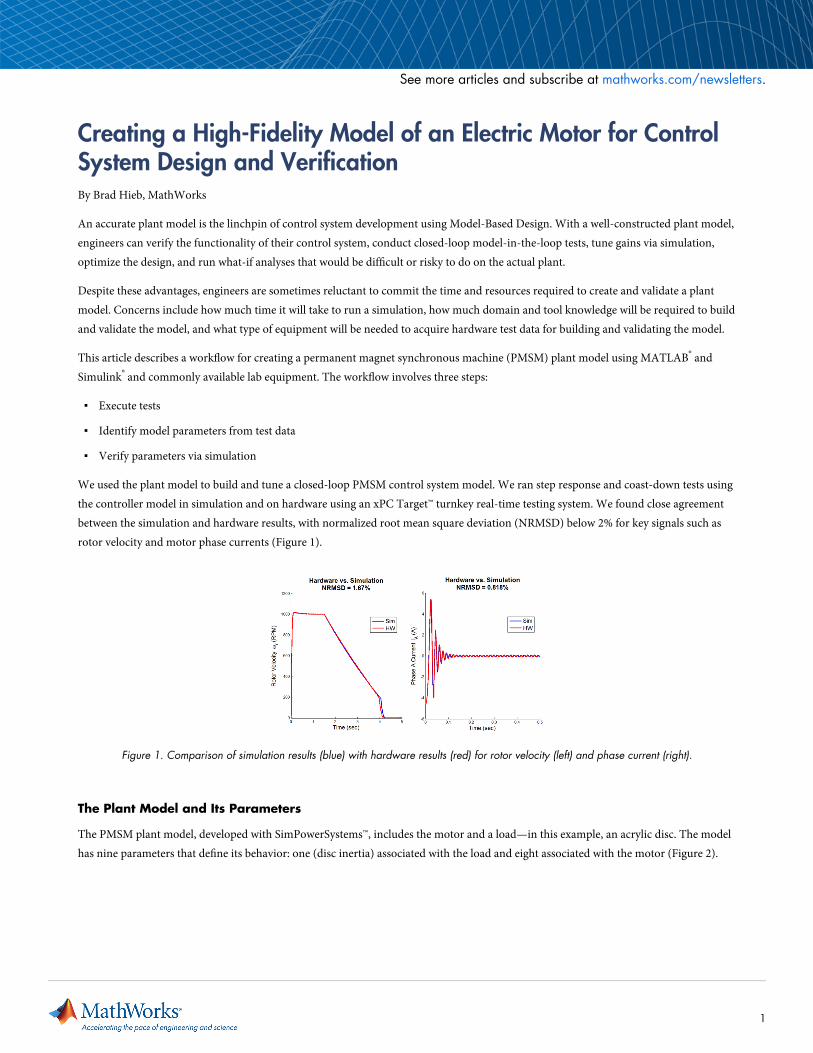
We used the plant model to build and tune a closed-loop PMSM control system model. We ran step response and coast-down tests usingthe controller model in simulation and on hardware using an xPC Target™ turnkey real-time testing system. We found close agreementbetween the simulation and hardware results, with normalized root mean square deviation (NRMSD) below 2% for key signals such asrotor velocity and motor phase currents (Figure 1).

Figure 1. Comparison of simulation results (blue) with hardware results (red) for rotor velocity (left) and phase current (right).

The Plant Model and Its Parameters

The PMSM plant model, developed with SimPowerSystems™, includes the motor and a load—in this example, an acrylic disc. The modelhas nine parameters that define its behavior: one (disc inertia) associated with the load and eight associated with the motor (Figure 2).

See more articles and subscribe at mathworks.com/newsletters.

1

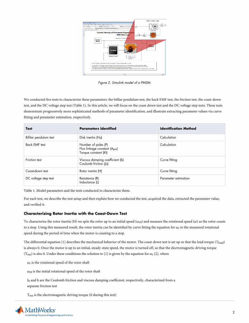
Figure 2. Simulink model of a PMSM.

We conducted five tests to characterize these parameters: the bifilar pendulum test, the back EMF test, the friction test, the coast-downtest, and the DC voltage step test (Table 1). In this article, we will focus on the coast-down test and the DC voltage step tests. These testsdemonstrate progressively more sophisticated methods of parameter identification, and illustrate extracting parameter values via curvefitting and parameter estimation, respectively.

Test Parameters Identified Identification Method

Bifilar pendulum test Disk inertia (Hd) Calculation

Back EMF test Number of poles (P)Flux linkage constant (Apm)Torque constant (Kt)

Calculation

Friction test Viscous damping coefficient (b)Coulomb friction (J0)

Curve fitting

Coast-down test Rotor inertia (H) Curve fitting

DC voltage step test Resistance (R)Inductance (L)

Parameter estimation

Table 1. Model parameters and the tests conducted to characterize them.

For each test, we describe the test setup and then explain how we conducted the test, acquired the data, extracted the parameter value,and verified it.

Characterizing Rotor Inertia with the Coast-Down Test

To characterize the rotor inertia (H) we spin the rotor up to an initial speed (ωr0) and measure the rotational speed (ω) as the rotor coaststo a stop. Using this measured result, the rotor inertia can be identified by curve fitting the equation for ωr to the measured rotationalspeed during the period of time when the motor is coasting to a stop.

The differential equation [1] describes the mechanical behavior of the motor. The coast-down test is set up so that the load torque (Tload)is always 0. Once the motor is up to an initial, steady-state speed, the motor is turned off, so that the electromagnetic driving torque(Tem) is also 0. Under these conditions the solution to [1] is given by the equation for ωr [2], where

ωr is the rotational speed of the rotor shaft

ωr0 is the initial rotational speed of the rotor shaft

J0 and b are the Coulomb friction and viscous damping coefficient, respectively, characterized from aseparate friction test

Tem is the electromagnetic driving torque (0 during this test)

2

Tload is the load torque (0 during this test)

Conducting the Test and Acquiring the Data

In the lab we created an open-loop Simulink test model to drive the motor to an initial speed of 150 radians per second, at which time themotor drive was turned off and the rotor coasted to a stop. Throughout the test the model captured the output of the rotational speedsensor. Using Simulink Coder™ and xPC Target, we deployed this model to an xPC Target turnkey real-time system. We executed themodel using xPC Target, and imported the rotor speed data into MATLAB for analysis.

Extracting and Verifying the Parameter Values

After running the tests, we plotted the measured speed data in MATLAB and used Curve Fitting Toolbox™ to fit equation [2] for therotor angular velocity (ωr) to the measured speed data while the rotor was coasting to a halt. Using the value of H from the curve fit, weevaluated equation [2] from the point at which the motor started coasting and plotted the results with the original test data (Figure 3). AsFigure 3 shows, equation [2] with the value of H from the curve fit closely predicts the motor speed during the coast-down test.

Figure 3. Plot of rotor velocity during the coast-down test. Blue = hardware test results; red = curve fitting results.

We used a model to verify our parameter identification result. Using the rotor inertia value obtained from the coast-down test(3.2177e-06 Kg m^2 in our PMSM model), we ran a simulation of the coast-down test in Simulink. We then compared and plotted thesimulated results with the measured results (Figure 4). The results matched closely, with a normalized root mean square deviation(NRMSD) of about 2%.

3

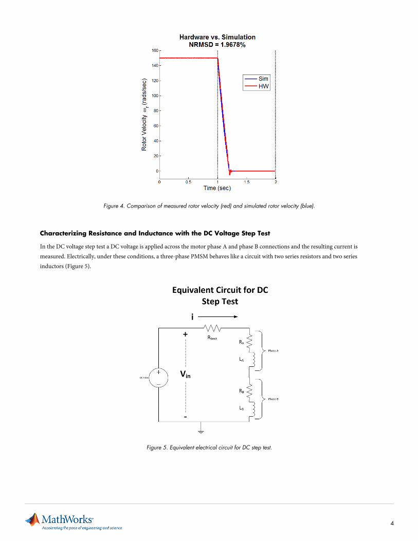
Figure 4. Comparison of measured rotor velocity (red) and simulated rotor velocity (blue).

Characterizing Resistance and Inductance with the DC Voltage Step Test

In the DC voltage step test a DC voltage is applied across the motor phase A and phase B connections and the resulting current ismeasured. Electrically, under these conditions, a three-phase PMSM behaves like a circuit with two series resistors and two seriesinductors (Figure 5).

Figure 5. Equivalent electrical circuit for DC step test.

4

The measured current (i) is used to find the resistance and inductance parameter values. During the test the rotor is held motionless toavoid complicating the analysis with back EMF waveforms, which tend to oppose the current flow. To avoid burning out the motor withthe rotor motionless, a current limiting resistor (Rlimit) is added and a step pulse rather than a steady DC voltage is used.

Conducting the Test and Acquiring the Data

We again used xPC Target and an xPC Target turnkey real-time system to conduct the test. In Simulink we developed a model thatproduced a series of 24-volt pulses roughly 2.5 milliseconds in duration. We deployed this model to our xPC Target system usingSimulink Coder, and applied the voltage pulse across the phase A and phase B terminals of the PMSM. We measured the applied voltageand the current flowing through the motor using an oscilloscope, and using Instrument Control Toolbox™ we read the measured datainto MATLAB, where we plotted the results (Figure 6).

Figure 6. Voltage (top) and current (bottom) for a pulse in the DC voltage step test.

Extracting and Verifying the Parameter Values

Extracting the phase resistance from the measured data required only the application of Ohm’s law (R = V/I) using the steady-statevalues for voltage and current. For the PMSM we calculated the resistance as 23.26 volts / 2.01 amps = 11.60 ohms. By subtracting 10ohms (the value of the current limiting resistor), and dividing the result by 2 to account for the two-phase resistances in series, wecalculated the motor phase resistance to be 0.8 ohms.

Characterizing the inductance required a more sophisticated approach. At first glance, it looks as if we could have used curve fitting, aswe did when characterizing the rotor inertia. However, due to the internal resistance of the DC supply, the measured DC voltage decaysfrom an initial value of 24 volts at the start of the test, when the current into the circuit is 0, to a steady-state value of 23.26 volts after thecurrent is flowing in the circuit. Because the input voltage is not a pure step signal, the results from curve fitting the solution to the seriesRL circuit equation would not be accurate.

To overcome this difficulty we opted for a more robust approach using parameter estimation and Simulink Design Optimization™. Theadvantage of this approach is that it requires neither a pure step input nor curve fitting.

We modeled the motor’s equivalent series RL circuit with Simulink and Simscape™ (Figure 7). Simulink Design Optimization applied themeasured voltage as an input to the model, and with the value of the limiting resistor (Rlimit) and the motor phase resistance (R_hat)

5

already known, estimated the value of the inductance (L_hat) to make the current predicted by the model match the measured currentdata as closely as possible.

Figure 7. Simscape model of the motor’s equivalent circuit.

To verify the values that we had obtained for phase resistance (0.8 ohms) and inductance (1.15 millihenries), we plugged the values intoour PMSM model and stimulated the model with the same input that we used to stimulate the actual motor. We compared thesimulation results with our measured results (Figure 8). The results matched closely, with an NRMSD of about 3%.

Figure 8. Comparison of measured results (blue) with simulation results (red) for voltage (top) and current (bottom).

Using the Plant Model to Design the Controller

After identifying and verifying all key parameters, our PMSM plant model was ready to use in the development of the motor controller.We used Simulink Design Optimization to tune the proportional and integral gains of the controller’s outer loop, the velocity regulator.We ran closed-loop simulations to verify the functionality of the controller model, and used Simulink Coder to generate code from themodel, which we deployed to an xPC Target turnkey real-time target machine.

6

As a final controller verification step, we ran step response and coast-down simulations in Simulink and hardware tests using thedeployed controller code on an xPC Target turnkey real-time system. We compared simulation and hardware test results for rotorvelocity and phase current, and once again found close agreement between the model and the hardware, with NRMSD below 2% in bothcases (Figure 9).

Figure 9. Comparison of simulation results (blue) with hardware results (red) for rotor velocity (left) and phase current (right).

Summary

Development of the PMSM plant model highlighted two parameter identification tests. Data was acquired via a sensor for thecoast-down test, and with Instrument Control Toolbox via an oscilloscope for the DC voltage step test. We extracted data via curvefitting for the coast-down test and parameter estimation for the DC voltage step test. We verified all parameter values by comparingsimulation results against measured test data, which enabled us to produce a plant model that we could trust as we developed and tunedthe controller.

All this work can be done early in the development process, well before embedded code is generated for the control system, enablingengineers to find and eliminate problems with the requirements and the design before hardware testing begins. These benefits typicallyfar outweigh the costs associated with creating the plant model, particularly if the model can be reused on other projects.

We would like to acknowledge the contribution of Professor Heath Hofmann of the University of Michigan, who recommended testprocedures for characterizing a PMSM and allowed us to use his lab facilities for the initial phase of this project.

Products Used

▪ MATLAB

▪ Simulink

▪ Curve Fitting Toolbox

▪ Instrument Control Toolbox

▪ SimPowerSystems

▪ Simscape

▪ Simulink Coder

▪ Simulink Design Optimization

▪ xPC Target

Learn More

▪ Webinar: A Simulink Real-Time Testing Solution for Power

Electronics and Motor Control (45:08)

▪ Webinar: Embedded Code Generation for AC Motors

(50:56)

▪ Video: Parameterizing and Verifying a Permanent Magnet

Synchronous Motor Model (37:16)

See more articles and subscribe at mathworks.com/newsletters.

Published 201392130v00

mathworks.com© 2013 The MathWorks, Inc. MATLAB and Simulink are registered trademarks of The MathWorks, Inc. See www.mathworks.com/trademarksfor a list of additional trademarks. Other product or brand names may be trademarks or registered trademarks of their respective holders.

7