Issues in the credit risk modeling of retail markets

Linda Allena,1

Gayle DeLongb,*

Anthony Saundersc,2

a Zicklin School of Business, Baruch College, One Bernard Baruch Way, Box B 10-225, New York, NY, 10010 USA

b Zicklin School of Business, Baruch College, One Bernard Baruch Way, Box B 10-225, New York, NY, 10010 USA

c John M. Schiff Professor of Finance, Stern School of Business, New York University, 44 West Fourth Street, New York, New York, USA

____________________________________________________________________________

Abstract

We survey the most recent BIS proposals for the credit risk measurement of retail credits in capital regulations. We also describe the recent trend away from relationship lending toward transactional lending in the small business loan arena. These trends create the opportunity to adopt more analytical, data-based approaches to credit risk measurement. We survey proprietary credit scoring models (such as Fair Isaac), as well as options-theoretic structural models (such as KMV and Moody’s RiskCalc), and reduced-form models (such as Credit Risk Plus). These models allow lenders and regulators to develop techniques that rely on portfolio aggregation to measure retail credit risk exposure.

JEL classifications: G21; G28

Keywords: Banks; Government policy and regulation ____________________________________________________________________________

1 Tel.: +1-646-312-3463, e-mail: Linda_Allen@baruch.cuny.edu.* Corresponding author. Tel: +1-646-312-3493; fax: +1-646-312-3451; e-mail: Gayle_DeLong@baruch.cuny.edu.2 Tel: +1-212-998-0711, e-mail: ASaunder@stern.nyu.edu.

Issues in the credit risk modeling of retail markets

1. Introduction

Retail credit markets offer special challenges to practitioners, regulators, and academics

alike. Because of the special features of the retail market, one cannot analyze small retail loans

by simply downsizing the models used to analyze large wholesale loans. The retail credit market

provides funds to small, typically unrated borrowers. The relatively small size of each loan

implies that the absolute size of the credit risk on any individual loan is minimal. Losses on any

single retail loan will not cause a bank to become insolvent. Thus, the cost per loan of

determining the credit risk of retail loans is often greater than the benefit in terms of loss

avoidance, and ascertaining the credit risk on an individual retail loan basis may not be

worthwhile. Moreover, the propensity to default or become delinquent may be affected by social

factors, as well as standard economic and business-cycle effects. Gross and Souleles (2002) find

that retail borrowers were increasingly willing to default on their credit card debt between 1995

and 1997, in large part because of the falling social, information, and legal costs of default.

The wholesale market, on the other hand, deals with large, negotiated loans to borrowers

who often have credit ratings. These large loans often are syndicated, thereby creating a

secondary market that does not exist for retail bank loans. Loan prices are available for

syndicated loans trading in the secondary market.2 In contrast, individual retail loans are not

frequently traded so there is no history of daily price fluctuations upon which to build future price

or value expectations. While securitization allows for the trading of mortgage, credit card, or

auto loan portfolios, little is known about the risk characteristics of individual retail loans. Risk

characteristics such as the probability of default (PD), the loss given default (LGD), exposure at

default (EAD), and default correlations differ from wholesale commercial loan markets so that

the parameters used for wholesale loan markets cannot be used reliably for retail markets; see

RMA (2000). Although several models exist to guide the providers of wholesale loans,3 the body

of research on retail credit risk measurement is quite sparse. A survey of what we know, and

perhaps more important, what we don’t know in the area of retail credit risk measurement is the

topic of this paper.

In this paper, we examine credit risk at the retail level. In Section 2, we begin with an

overview of the proposals from the Bank for International Settlements (BIS) concerning

international bank capital requirements for retail credit. In Section 3, we examine some 2 For example, Loan Pricing Corporation maintains a database that marks to market approximately 2,000 syndicated bank loans on a daily basis using dealer bid/ask quotes.3 For more comprehensive coverage of the models, see Saunders and Allen (2002).

traditional models of credit risk measurement – expert systems, rating systems, and credit

scoring. In Section 4, we compare two major approaches to small business lending: relationship

lending, which entails significant private information produced by bank monitoring in the context

of a long-standing bank-borrower business relationship, and transactional lending, which does not

incorporate a significant expenditure of resources by the bank on obtaining private information

about the borrower. Each of these forms of retail lending offers unique problems in the

measurement of the retail loan’s credit risk. For example, it may be more appropriate to measure

the credit risk of the entire bank-borrower relationship, rather than concentrating on the stand-

alone credit risk of an individual relationship bank loan. In Section 5, we discuss how one may

apply new techniques of credit risk measurement to retail loans, and the paper concludes in

Section 6.

2. BIS Basel New Capital Accord

The Bank for International Settlements (BIS (2001), p. 55) defines retail credit as

“homogeneous portfolios comprising a large number of small, low value loans with either a

consumer or business focus, and where the incremental risk of any single exposure is small.”

These types of loans include loans to individuals such as credit cards, residential mortgages, and

home equity loans as well as other personal loans such as educational or auto loans. Small

business loans could also be included as long as the bank treats these facilities the same way it

treats other retail credits.

The Basel Committee on Banking Supervision is responsible for proposing capital

requirements for internationally active banks. Typically, regulators around the world adopt the

guidelines put forth by the committee, even if they are not from one of the 13 nations represented

on the committee. The committee first proposed the Basel New Capital Accord, also known as

Basel II, in December 2001, with revisions in July 2002 and April 2003. More revisions are

likely before the final adoption of the accord. By year-end 2006, Basel II is expected to replace

the original Basel Accord, which was implemented in 1992. The proposals allow banks to choose

among several approaches to determine their capital requirements to cover credit risk. The

standardized approach allows less sophisticated banks to use external credit ratings to classify the

bank’s assets into risk classes. Over time, banks are expected to evolve to the internal ratings-

based approaches (foundation and advanced), which rely on the bank’s own experience in

determining the risk characteristics of various asset classes. For example, the foundation IRB

approach for corporate, sovereign, and bank exposures allows banks to provide estimates of

probability of default but requires banks to use supervisory estimates of loss given default,

1

exposure at default, and maturity. The advanced IRB approach for such exposures allows banks

to provide estimates of PD, LGD, and EAD and requires banks to provide estimates of maturity.

The treatment of small- and medium-size enterprise (SME) exposures is viewed as

especially important in countries where small/medium-size firms comprise a significant

component of the industrial sector (e.g., Germany). SME borrowers are defined by the Basel

Committee as those with less than €50 million in annual sales. Such exposures are allowed to

have up to 20% lower capital requirements than exposures to larger firms. Furthermore, banks

that treat their SME exposures as a homogeneous portfolio (in the same way as they treat their

retail exposures) are permitted to apply the retail IRB capital requirements to the portfolio as long

as the exposure to the bank of any individual SME is less than €1 million.

Banks opting to use the standardized approach for their retail exposures would continue

to use the 8% capital requirement (under the original Basel Capital Accord) to calculate the

minimum capital requirement. However, the risk weights would vary for different classes of

retail loans. Specifically:

K = EAD x RW x 0.08, (1)

where K = capital requirement,

EAD = exposure at default of the retail assets, and

RW = risk weight, which is set equal to 35% for residential mortgages and 75% for other

retail credit, including loans to small and medium enterprises.

If a bank chooses the IRB approach for retail credit exposures, the bank must estimate PD

and LGD, as well as EAD. No explicit maturity factor is included in the functions, since the

correlation assumptions for the various types of retail exposures (shown below) reflect the

average maturity of the retail exposures. Moreover, only the advanced IRB approach exists for

retail credit. If a bank adopts the IRB approach, the committee expects the bank eventually to

implement the IRB advanced approach for the entire bank, with the possible exceptions of the

smallest portfolios. Furthermore, the committee expects the bank to maintain that approach

unless a significant circumstance such as a divestiture occurs.

The proposals in April 2003 include several internal ratings-based models for retail credit

risk measurement. For the three types of retail credit (residential mortgages, revolving credit,

and other retail loans), these models specify the risk-weighted assets, as well as the amount of

capital banks must hold for each portfolio composed of retail credit exposures. The new Basel

Capital Accord proposal (BIS (2003)) details each model. For all retail exposures, banks provide

assessments of the probability of default (PD) as well as loss given default (LGD).

2

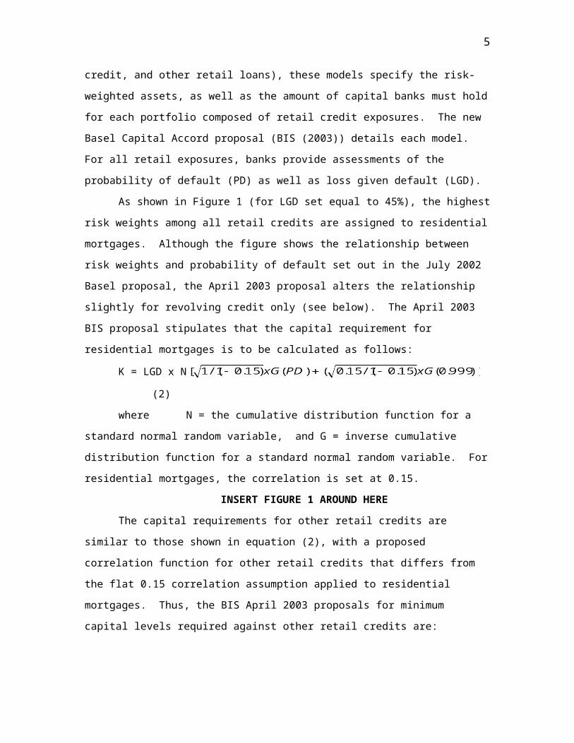
As shown in Figure 1 (for LGD set equal to 45%), the highest risk weights among all

retail credits are assigned to residential mortgages. Although the figure shows the relationship

between risk weights and probability of default set out in the July 2002 Basel proposal, the April

2003 proposal alters the relationship slightly for revolving credit only (see below). The April

2003 BIS proposal stipulates that the capital requirement for residential mortgages is to be

calculated as follows:

K = LGD x N

(2)

where N = the cumulative distribution function for a standard normal random variable,

and G = inverse cumulative distribution function for a standard normal random variable. For

residential mortgages, the correlation is set at 0.15.

INSERT FIGURE 1 AROUND HERE

The capital requirements for other retail credits are similar to those shown in equation

(2), with a proposed correlation function for other retail credits that differs from the flat 0.15

correlation assumption applied to residential mortgages. Thus, the BIS April 2003 proposals for

minimum capital levels required against other retail credits are:

K = LGD x N (3)

where N = the cumulative distribution function for a standard normal random variable,

G = inverse cumulative distribution function for a standard normal random variable, and R =

correlation. The proposed correlation expression is:

R = 0.02 x

(4)

The impact of the correlation expression in equation (4) is to decrease the correlation coefficient

at higher levels of PD. Table 1 shows that the risk weight for other retail credits is slightly above

the risk weight for residential mortgages at low levels of PD (below 0.50%) but decreases

(relative to the risk weight for residential mortgages) at higher levels of PD, as a result of the

assumed inverse relationship between correlation and PD in equation (4).4 Thus, as PD exceeds

0.50%, the correlation on other retail credits calculated using equation (4) falls below 0.15,

thereby lowering the risk weight and the bank’s capital requirement for other retail credit as

compared to residential mortgages.5 The assumption of an inverse relationship between PD and

correlation is quite controversial. Most academic studies find a direct relationship such that 4 Although the data in Table 1 come from the July 2002 proposal, capital requirements for revolving credit are only slightly higher in the April 2003 proposal as explained later in this section.

3

higher quality, low PD firms tend to have less systematic risk and therefore lower correlations,

whereas lower quality, high PD firms are more subject to market shocks and therefore have

higher correlations. See Allen and Saunders (2003) for a discussion.

INSERT TABLE 1 AROUND HERE

The third model is proposed for the measurement of bank capital requirements for

revolving credit. As shown in Figure 1, revolving credit has the lowest capital requirement of all

three retail credits. Although the figure shows the model proposed in July 2002, the model was

modified in April 2003 so that capital requirements are slightly higher for revolving credit (see

below). Even under the new proposal, revolving credit has the lowest capital requirement. The

lower capital requirements for revolving credit reflect a belief that although retail products have

higher rates of estimated default and higher loss given default (LGD), the correlation among retail

products is lower than among wholesale products. (See RMA (2000).) This assumption is

reflected in the proposed regulations in two ways. First, the correlation expression for revolving

credits is lower (at each level of PD) than the correlation for other retail credits (and lower than

the correlation for residential mortgages at most levels of PD). Second, the capital requirement is

lowered for revolving exposures to allow 75% of expected losses to be covered by future income.

The 75% exemption is down from 90% proposed in July 2002, so that capital requirements for

revolving exposures increased slightly in April 2003 over the July 2002 proposals. Thus, the

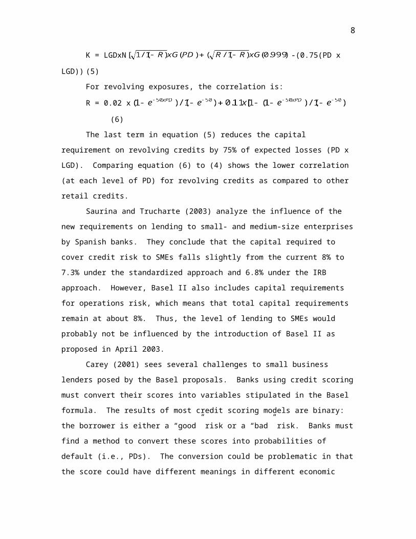
April 2003 IRB proposals for minimum capital requirements for revolving credit are:

K = LGDxN -(0.75(PD x LGD))

(5)

For revolving exposures, the correlation is:

R = 0.02 x

(6)

The last term in equation (5) reduces the capital requirement on revolving credits by 75%

of expected losses (PD x LGD). Comparing equation (6) to (4) shows the lower correlation (at

each level of PD) for revolving credits as compared to other retail credits.

Saurina and Trucharte (2003) analyze the influence of the new requirements on lending

to small- and medium-size enterprises by Spanish banks. They conclude that the capital required

to cover credit risk to SMEs falls slightly from the current 8% to 7.3% under the standardized

approach and 6.8% under the IRB approach. However, Basel II also includes capital

requirements for operations risk, which means that total capital requirements remain at about 8%. 5 That is, the risk weight and capital requirements for both residential mortgages and other retail credits increase as PD increases (holding LGD constant), but the risk weight for residential mortgages increases by more than the risk weight for other retail credits at higher PD levels.

4

Thus, the level of lending to SMEs would probably not be influenced by the introduction of Basel

II as proposed in April 2003.

Carey (2001) sees several challenges to small business lenders posed by the Basel

proposals. Banks using credit scoring must convert their scores into variables stipulated in the

Basel formula. The results of most credit scoring models are binary: the borrower is either a

“good” risk or a “bad” risk. Banks must find a method to convert these scores into probabilities

of default (i.e., PDs). The conversion could be problematic in that the score could have different

meanings in different economic settings. That is, the same score could represent vastly different

probabilities of default depending on the state of the economy. Data pose another challenge. The

accord requires banks to record how well their models prepared them for losses. That is, the

banks must keep a record of projected losses and compare the projections with actual losses over

time. This requirement forces banks to implement new tracking systems, since according to

RMA (2000), many banks have information on retail loans for the most recent 48 months at most.

Moreover, even less sophisticated banks will be required to perform complicated, data-intensive

back-testing of their models.

Another problem could be the different assessments banks assign to the same type of

product. Since individual loan risk assessment is not economically feasible, banks group their

retail loans into portfolios along product lines. RMA (2000) gathered information from 11 U.S.

and Canadian banks on how they measure credit risk for retail products and identified eight

distinct retail product lines: first mortgages, credit cards, leasing, student loans, other secured

retail loans, other unsecured retail loans, home equity loans, and home equity lines of credit. If a

bank assesses a higher probability of default or loss given default for a particular product line,

then that bank must hold more capital than a bank that assigns a lower probability. The RMA

study examined how banks assigned two important characteristics of risk: expected default

frequency and loss given default along retail product lines. Overall, loss given default tended to

be higher for retail products (except first mortgages) than for wholesale loans, but correlations

among retail loans tended to be lower. Banks assigned similar risk characteristics for six of the

products: first mortgages, credit cards, leasing, student loans, other secured, and other unsecured

loans. Banks differed mainly on their assessments of two other products, namely, home equity

loans and home equity lines of credit. In assigning these risk characteristics, banks often made

use of the traditional models of credit risk measurement that will be surveyed in the next section.

3. Traditional Approaches to Credit Risk Measurement

5

Traditional methods focus on estimating the probability of default (PD) and typically

specify “default” to include bankruptcy filing, default, or liquidation. We consider three broad

categories of traditional models used to estimate PD: (1) expert systems, including artificial

neural networks; (2) rating systems; and (3) credit scoring models.

3.1 Expert Systems

Historically, bankers have relied on loan officer expert systems such as the 5 Cs of credit

to assess credit quality: character (reputation), capital (leverage), capacity (earnings volatility),

collateral, and cycle (macroeconomic) conditions. Evaluation of the 5 Cs is performed by human

experts, who may be inconsistent and subjective in their assessments. Moreover, traditional

expert systems specify no weighting scheme that would consistently order the 5 Cs in terms of

their relative importance in forecasting PD. Thus, artificial neural networks have been introduced

to develop more objective expert systems. A neural network is “trained” using historical

repayment experience and default data. Structural matches are found that coincide with

defaulting firms and then used to determine a weighting scheme to forecast PD. Each time the

neural network evaluates the credit risk of a new loan opportunity, it updates its weighting

scheme so that it continually “learns” from experience. Thus, neural networks are flexible,

adaptable systems that can incorporate changing conditions into the decision-making process.

One type of neural network is the multi-layer perceptron network.6 A multi-layer

perceptron network starts with a series or “layer” of inputs and ends with a layer of outputs.

Between these two layers are several layers of information processing points, or “neurons,” that

assist in determining the weight each input should receive. In the case of credit decisions, the

input layer could be several financial ratios and the output layer could be whether or not the

borrower defaults. Using the inputs of loans with known outputs, the network experiments with

various weights until the weighting system with the least error emerges. The network then uses

these weights to predict the outcomes of loans with particular inputs.

Empirical tests of the accuracy of neural networks produce mixed results. Kim and

Scott (1991) use a supervised artificial neural network to predict bankruptcy in a sample of 190

Compustat firms. While the system performs well (87% prediction rate) during the year of

bankruptcy, its accuracy declines markedly over time, showing only a 75%, 59%, and 47%

prediction accuracy one year prior, two years prior, and three years prior to bankruptcy,

respectively. Altman et al. (1994) examine 1,000 Italian industrial firms from 1982-1992 and

find that neural networks have about the same level of accuracy as do credit scoring models.

6 For a good overview of multi-layer perceptron networks, see Morton (2003) as well as Hawley et al. (1990)

6

Podding (1994), using data on 300 French firms collected over three years, claims that neural

networks outperform credit scoring models in bankruptcy prediction. However, he finds that not

all artificial neural systems are equal, noting that the multi-layer perceptron (or back propagation)

network is best suited for bankruptcy prediction. Yang et al. (1999) uses a sample of oil and gas

company debt to show that the back propagation neural network obtained the highest

classification accuracy overall, when compared to the probabilistic neural network and

discriminant analysis. However, discriminant analysis outperforms all models of neural networks

in minimizing type 2 classification errors, that is, misclassifying a good loan as bad.

During “training” the neural network fits a system of weights to each financial variable

included in a database consisting of historical repayment/default experiences. However, the

network may be “overfit” to a particular database if excessive training has taken place, thereby

resulting in poor out-of-sample estimates. Moreover, neural networks are costly to implement

and maintain. Because of the large number of possible connections, the neural network can grow

prohibitively large rather quickly. Finally, neural networks suffer from a lack of transparency.

Since there is no clear economic interpretation that can be attached to the hidden intermediate

steps, the system cannot be checked for plausibility and accuracy. Structural errors will not be

detected until PD estimates become noticeably inaccurate.

3.2 Internal Rating Systems

The Office of the Comptroller of the Currency (OCC) in the United States has long

required banks to use internal ratings systems to rank the credit quality of loans in their portfolios.

However, the rating system has been rather crude, with most loans rated as Pass/Performing and

only a minority of loans differentiated according to the four non-performing classifications (listed

in order of declining credit quality): other assets especially mentioned, substandard, doubtful, and

loss. Similarly, the National Association of Insurance Commissioners requires insurance

companies to rank their assets using a rating schedule with six classifications corresponding to

the following credit ratings: A and above, BBB, BB, B, below B, and default.

Many banks have instituted internal ratings systems in preparation for the BIS New

Capital Accord scheduled for implementation in 2006. The architecture of the internal rating

system can be one-dimensional, in which an overall rating is assigned to each loan based on the

probability of default (PD), or two-dimensional, in which each borrower’s PD is assessed

separately from the loss severity of the individual loan. Treacy and Carey (2000) estimate that

60% of the financial institutions in their survey had one-dimensional rating systems, although

7

they recommend a two-dimensional system. Moreover, the BIS (2000) found that banks were

better able to assess their borrowers’ PD than their loss given default.7

Treacy and Carey (2000) in their survey of the 50 largest U.S. bank holding companies

and the BIS (2000) in its survey of 30 financial institutions across the G-10 countries found

considerable diversity in internal ratings models. Although all used similar financial risk factors,

there were differences across financial institutions with regard to the relative importance of each

of the factors. Treacy and Carey (2000) found that qualitative factors played more of a role in

determining the ratings of loans to small and medium-size firms, with the loan officer chiefly

responsible for the ratings, in contrast with loans to large firms in which the credit staff primarily

set the ratings using quantitative methods such as credit-scoring models. Typically, ratings were

set with a one-year time horizon, although loan repayment behavior data were often available for

3-5 years.8

3.3 Credit Scoring Models

The most commonly used traditional credit risk measurement methodology is the

multiple discriminant credit scoring analysis pioneered by Altman (1968). Mester (1997)

documents the widespread use of credit scoring models: 97% of banks use credit scoring to

approve credit card applications, whereas 70% of the banks use credit scoring in their small

business lending. There are four methodological forms of multivariate credit scoring models: (1)

the linear probability model, (2) the logit model, (3) the probit model, and (4) the multiple

discriminant analysis model. All of these models identify financial variables that have statistical

explanatory power in differentiating defaulting firms from non-defaulting firms. Once the

model’s parameters are obtained, loan applicants are assigned a Z-score assessing their

classification as good or bad. The Z-score itself can be converted into a PD.

Credit scoring models are relatively inexpensive to implement and do not suffer from the

subjectivity and inconsistency of expert systems. Table 2 shows the spread of these models

throughout the world, as surveyed by Altman and Narayanan (1997). What is striking is not so

much the models’ differences across countries of diverse sizes and in various stages of

development but rather their similarities. Most studies found that financial ratios measuring

profitability, leverage, and liquidity had the most statistical power in differentiating defaulted

from non-defaulted firms.

7 To adopt the internal-ratings based advanced approach in the new Basel Capital Accord, banks must adopt a risk rating system that assesses the borrower’s credit risk exposure (LGD) separately from that of the transaction.8 A short time horizon may be appropriate in a mark to market model, in which downgrades of credit quality are considered, whereas a longer time horizon may be necessary for a default mode that considers only the default event. See Hirtle et al. (2001).

8

INSERT TABLE 2 AROUND HERE

One of the most widely used credit scoring systems was developed by Fair Isaac and Co.

Inc. (FICO). During the 1960s and 1970s, the firm created credit scoring systems tailored to meet

the needs of individual clients, mainly retail stores and banks in the United States. In the 1980s,

Fair Isaac serviced more industries, including insurance, as well as more countries in Europe.

During the 1990s, the firm developed products to evaluate credit of small businesses, including

trade credit (CreditFYI.com) in 1998 and loan credit (LoanWise.com) in 1999. Personal credit

evaluation became more accessible with the development of myfico.com in 2001. Customers can

determine their credit score directly using the Internet.

Credit scoring systems vary according to the information they evaluate and how they

evaluate it. For example, Fair Isaac assesses credit reports and credit history to determine a score

that ranges between 300 and 850. The assessment considers all outstanding debt such as

mortgage loans and credit card balances as well as the proportion of balances to credit limits on

credit cards. Payment history, such as whether and how often an individual was late in making

payments as well as the length of the credit history, is also included. The evaluation does not

include characteristics that could bias a lender such as race, religion, national origin, gender, or

marital status. However, the evaluation also ignores salary and occupation, so that a person with

a good, steady income and a history of always paying his/her credit card receivables may not

achieve a perfect score.

Some shortcomings of credit scoring models are data limitations and the assumption of

linearity. Using analysis of variance, discriminant analysis fits a linear function of explanatory

variables to the historical data on default and repayment. Moreover, as shown in Table 2, the

explanatory variables are predominantly limited to balance sheet data. These data are updated

infrequently and are determined by accounting procedures that rely on book, rather than market

valuation. Finally, there is often limited economic theory as to why a particular financial ratio

would be useful in forecasting default.

Recent modifications of credit scoring have given banks the opportunity to treat small

business loans as retail credit. That is, before the application of credit scoring to small business

loans, such loans were usually made on a relationship basis. The following section explains the

differences and implications of relationship versus transactional lending.

4. Pricing of Small Business Loans

Loans to small businesses differ from loans to large businesses. Peterson (1999) suggests

three major differences. First, since lenders face fixed costs in lending, lending to small firms is

9

by definition more expensive per dollar lent. Second, the relationship between the

owner/manager of a small firm and a small bank is often very close. Finally, small firms are

more informationally opaque. Because of these structural features, banks can choose how they

treat their retail credits for risk analysis purposes. Some (usually small) banks attempt to treat

their small business customers the same way they treat their large commercial borrowers.

Balance sheet and income statement data are collected and analyzed. When such data are not

available, as is often the case in small businesses, modifications are made. Analysis consisted of

bypassing the need for “hard” data by building a relationship with the owner/manager and

therefore obtaining the necessary information to assess the creditworthiness of the client. Such

relationship lending differs markedly from the current trend toward transactional lending.

In contrast to relationship small business loans, transactional loans are pooled together

and treated as if they are a homogeneous portfolio. Thus, rather than ascertaining the risk

characteristics of a particular borrower, the bank analyzes the overall PD and LGD of the entire

portfolio of transactional retail loans. This approach to small business lending is used most often

by large banks, whereas smaller banks typically specialize in relationship lending to small

businesses; see Berger and Udell (1995) and Peterson and Rajan (1994).

4.1 Relationship Lending

Banks that engage in relationship lending often obtain information about their clients that

is proprietary. Banks form a special bond with their clients either by serving them over time or

providing many products simultaneously (see Boot (2000)). Peterson (1999) suggests that

relationship lending is similar to taking an equity stake in a firm. Berlin and Mester (1998) show

how relationship lending can lead to loan rate smoothing over time. Relationship lending is

based on “soft” data such as personal connections and reputation.

4.1.1 Pricing Relationship Loans

Most research on the pricing of small business loans looks at the length and breadth of

the relationship between the bank and its client. The research then determines how that

relationship affects the price of the loan. A study by Berger and Udell (1995) shows that

relationship banking results in new borrower’s subsidizing established borrowers. That is, banks

charge clients with whom they have had long-term relationships lower interest rates than new

clients. However, Peterson and Rajan (1994) do not find a statistically significant relationship

between interest rates and the length of a bank-client relationship.

4.1.2 Drawbacks of Relationship Lending

Relationships are expensive to establish and maintain. Time and resources must be

readily available for the recipients of relationship loans. While small banks have a competitive

10

advantage in making relationship loans (see Berger and Udell (1996)), the banks themselves may

remain small since they cannot generate enough business to become large. Relationships are

particularly expensive for large banks, since large banks have sufficient capital to make large

loans. Spending time to cultivate small accounts is simply not an efficient use of resources when

the same amount of effort can result in a much larger loan.

Moreover, the special relationship between the bank and client may not maximize profits

for the bank. Berlin and Mester (1998) show that loan rate smoothing in light of interest rate

shocks can be profitable for banks that engage in relationship lending, but such smoothing as a

result of credit risk shocks can be detrimental to the profitability of lending institutions.

Relationship lending could also lead to discrimination. Cavalluzzo et al. (2002) examine

credit granted to small businesses based on the gender, race, and ethnicity of the owner. Even

after controlling for personal and business credit histories, the authors find denial rates for black

men are substantially higher than for white men. Also, women tend to receive fewer loans in

concentrated markets. However, competition within a local banking area appears to lower

discrimination.

Despite the costs, large banks have recently taken an interest in small business lending.

This interest stems in part from the pressure of disintermediation that caused large banks to lose

business as many of their more lucrative clients go directly to the capital markets. Moreover, the

interest could reflect a desire to obtain higher, more consistent profits. Basset and Brady (2001)

report that between 1985 and 2000, the net interest margins of banks was consistently about 1%

higher for small banks than for large banks, suggesting that small banks are able to extract more

profit from the loans they make. During the same time period, small banks experienced a gradual

increase in return on assets (ROA) from approximately 0.7% to 1.1%. The ROA for large banks

vacillated from a low of -0.4% in 1987 to 1.1% in 2000. Large banks therefore have an incentive

to capture part of the lucrative retail loan market. If large banks learn to make retail loans

efficiently, they might smooth their earnings and perhaps increase their net interest margins and

therefore revenues and profits. This interest in retail credit by large banks has spurred new ways

of making loans to small businesses, namely, transactional lending.

4.2 Transactional Lending

In contrast to relationship lending, transactional lending is based on portfolio risk

measurement tools, such as credit scoring (described in Section 3.3). Banks review loan

applications based on specific, quantifiable criteria. One widely used model is by Fair Isaac, and

another model is by SMEloan. Although credit scoring results may be quite inaccurate for

11

informationally opaque small business borrowers, banks anticipate a portfolio diversification

effect based on the average performance of the entire transactional loan portfolio.

Using its credit scoring model for individual consumers, Fair Isaac and Co. Inc.

developed its Small Business Scoring System (SBSS) in the early 1990s. The impetus for the

SBSS came from Robert Morris Associates (RMA), renamed the Risk Management Association,

a group representing credit risk managers from over 3,000 financial institutions. The

practitioners from RMA noticed that repayment of small business loans depended less on the

business itself than on the credit history of the founder. That is, an individual who repays debts is

likely to run a small business that repays its debts. RMA asked Fair Isaac to develop a model

based on RMA’s observations. Fair Isaac studied the data collected by 17 banks on 5,000 small

business loans. Fair Isaac analyzed hundreds of pieces of data collected on each loan and

determined that fewer than a dozen aspects of the borrower were important. These aspects

included total assets of the firm as well as the time in business. Fair Isaac also verified the

observations of the practitioners, namely, the characteristics of the owner – e.g., age, number of

dependents, and time at address – were more important than the business itself. In 2002, over

350 U.S. lenders used the system in the analysis of over 1 million credit decisions.

Banks that use credit scoring models appear to be more productive at lower costs.

Longenecker et al. (1997) report the results of Hibernia Corporation, which implemented credit

scoring in 1993. Before the implementation of credit scoring, seven loan officers processed 100

applications per month. By 1995, the same number of loan officers processed over 1,000

applications per month. The business loan portfolio increased from $100 million to $600 million

during the same time period. Moreover, the bank appeared to make fewer bad loans.

Feldman (1997) details the advantages of credit scoring. No face-to-face contact is

necessary, so the bank can be located anywhere and still make the loan. Documentation is

minimal, since only the credit history of the owner/borrower is reviewed. Review is therefore

much faster and probably results in lower costs. Loan losses could also be reduced as the

portfolio diversification effect results in fewer bad loans, on average. Lending volume can also

increase substantially.

One implication of credit scoring is that banks can lend to clients located farther and

farther away. Peterson and Rajan (2002) show that this long-distance lending stems from greater

bank productivity. Banks not only have more information, but they are able to use the

information they have more productively. The authors find that banks are providing small

business loans to clients who are located in ever more geographically dispersed regions. This

has the advantage of shielding the bank’s portfolio from the effects of imperfect geographic

12

diversification. Peterson and Rajan also show that banks are able to provide such geographically

diversified loans, because hard data concerning the clients are now available. Moreover, bank

productivity has increased.

Credit scoring also affords benefits to borrowers. Not only is credit more available, but

competition is also stronger, since more banks can cover wider areas of business. One

implication is that borrowers are no longer at the mercy of their local banks. Singletary (1995)

reports that “Now, small-business owners don’t have to grovel at the loan officer’s desk.”

One reason transaction loans are possible in the United States is that credit information is

readily available. Staten (2001) points out that the United States is unusual in promoting the

dissemination of credit reports. Such information allows lenders to assess the creditworthiness of

borrowers and therefore provides more credit in the economy. Not only is credit information

available, but it is more complete in that credit reports show both positive and negative history.

Some countries report only negative credit information on clients. Banks in “negative-only”

reporting countries, such as Australia, extend fewer loans. In a simulation, Staten (2001) reports

that at a targeted default rate of 4%, the negative-only model extended loans to 11% fewer

applicants than the full model. For every 100,000 applicants, the negative-only model extended

11,000 fewer loans. Since credit has a multiplier effect, the restriction of credit can lower the

growth of an economy.

4.2.1 Pricing Transactional Loans

Pricing relationship loans is vastly different from pricing transactional loans.

Transactional lending to small businesses is based on hard data, such as the credit history of the

borrowers (e.g., Fair Isaac model). Thus, lending rates can reflect credit scores for transactional

loans. For example, www.myFICO.com (2003) details the different national average home

lending rates for different levels of FICO scores. People with higher credit scores pay lower

interest rates. In another example, Feldman (1997) reports that Wells Fargo charges small

businesses a range of interest rates from prime plus 1% to prime plus 8% based on the business’s

credit score. Such gradations may not be possible if based on human judgment (i.e., expert

models) because of concerns about objectivity and consistency across borrowers.

4.2.2 Drawbacks of Transactional Lending

Despite the advantages of credit scoring for small business loans, Mester (1997) reports

that only 8% of banks with up to $5 billion in assets used scoring for small business loans.

Perhaps small banks are reluctant to switch to the use of quantitative models, fearing their

customers will miss the personal service of relationship lending.

13

Small banks apparently believe that they have advantages in making small business

loans. Indeed, Berger et al. (2001) show that large and foreign-owned banks tend to lend to large

urban clients, suggesting small banks have a competitive advantage in lending to small firms.

However, the study is based on data from Argentina. In other countries, such as the United

States, the availability of credit scoring models and the information needed to run the models may

suggest that we cannot generalize from the results of this study.

The special relationship between banks and their clients is lessened or lost when lending

becomes a transactional exercise. Banks are perceived as having superior information concerning

the clients to whom they lend. Dahiya et al. (2003) show that the market reacts negatively when

a bank sells a loan in its portfolio. The perception is well-founded: firms whose loans are sold

have a higher probability of bankruptcy than firms that do not. This special relationship is lost as

soon as the loans are treated as transactional retail exposures.

Transactional lending’s apparent lack of personal touch could also be overcome. Pine et

al. (1995) point out the use of hard data could lead to “mass customization.” Such customization,

however, relies on managing customer needs as opposed to managing products. Products could

be priced individually, just as Dell computers are individually created to suit individual needs but

are still able to turn the company a profit. Furthermore, relationship databases could be

established. This would combine the informational benefits of relationship lending with the cost

efficiencies of transactional lending.

As the retail loan market moves toward more analytical, data-based transactional lending,

there is increased opportunity to adapt modern models of credit risk measurement for the retail

market. In the next section, we briefly survey the two major strands of the literature – structural

models and reduced-form models of credit risk measurement.

5. Structural Models of Credit Risk Measurement

Modern methods of credit risk measurement can be traced to two alternative branches in

the asset pricing literature of academic finance: an options-theoretic structural approach

pioneered by Merton (1974) and a reduced-form approach, which uses intensity-based models to

estimate stochastic hazard rates, following a literature pioneered by Jarrow and Turnbull (1995),

Jarrow et al. (1997), Duffie and Singleton (1998), and Duffie and Singleton (1999). These two

schools of thought offer differing methodologies to accomplish the central task of all credit risk

measurement models – estimation of default probabilities. The structural approach models the

economic process of default, whereas reduced-form models decompose risky debt prices in order

to estimate the random intensity process underlying default. The two approaches can be

14

reconciled if asset values follow a random intensity-based process, with shocks that may not be

fully observed because of imperfect accounting disclosures. See Duffie and Lando (2001), Zhou

(1997), and Zhou (2001). No formal model for retail credit has yet used the reduced-form

approach, although one model, Credit Risk Plus, could be used for retail credit.

We first discuss the options-theoretic structural approach, which is used by KMV’s

Portfolio Manager and Moody’s RiskCalc to determine default probabilities. The KMV model

includes an adaptation for retail credit. We then discuss the possibilities of using the reduced-

form approach, which forms the basis for Credit Risk Plus.

Merton (1974) models equity in a levered firm as a call option on the firm’s assets with a

strike price equal to the debt repayment amount. If at expiration (coinciding to the maturity of

the firm’s short-term liabilities (usually one year), assumed to be composed of pure discount debt

instruments) the market value of the firm’s assets exceeds the value of its debt, the firm’s

shareholders will exercise the option to “repurchase” the company’s assets by repaying the debt.

However, if the market value of the firm’s assets falls below the value of its debt, the option will

expire unexercised and the firm’s shareholders will default.9 The PD until expiration is set equal

to the maturity date of the firm’s pure discount debt, typically assumed to be one year, though

Delianedis and Geske (1998) consider a more complex structure of liabilities. Thus, the PD until

expiration is equal to the likelihood that the option will expire out of the money. To determine

the PD, the call option10 can be valued using an iterative method to estimate the unobserved

variables that determine the value of the equity call option, in particular, A (the market value of

assets) and A (the volatility of assets). These values for A and A are then combined with the

amount of debt liabilities B that have to be repaid at a given credit horizon in order to calculate

the firm’s distance to default (defined to be or the number of standard deviations between

current asset values and the debt repayment amount). The higher the distance to default (denoted

DD), the lower the PD. To convert the DD into a PD estimate, Merton (1974) assumes that asset

values are log normally distributed. Since this distributional assumption is often violated in

practice, proprietary structural models use alternative approaches to map the DD into a PD

9 Assuming that shareholders are protected by limited liability, there are no costs of default, and absolute priority rules are strictly observed, then the shareholders’ payoff in the default region is zero.10 Using put-call parity, Merton (1974) values risky debt as a put option on the firm’s assets giving the shareholders the right, not the obligation, to sell the firm’s assets to the bondholders at the value of the debt outstanding. The default region then corresponds to the region in which the shareholders exercise the put option. The model uses equity volatility to estimate asset volatility, since both the market value of firm assets and asset volatility are unobservable. See Ronn and Verma (1986).

15

estimate. For example, KMV’s Portfolio Manager and Moody’s RiskCalc estimate an empirical

PD using historical default experience.11

5.1 KMV’s Portfolio Manager

Three inputs are needed for each loan to calculate the credit risk of a portfolio using

KMV’s Portfolio Manager: expected return, risk (variance), and correlation.

The distance to default (DD) for individual credits is converted into a probability of

default (PD) by determining the likelihood that the firm’s assets will traverse the debt boundary

point during the credit horizon period. KMV uses a historical database of default rates to

determine an empirical estimate of the PD, denoted expected default frequency (EDF). For

example, historical evidence shows that firms with DD equal to 4 have an average historical

default rate of 1%. Thus, KMV assigns an EDF of 1% to firms with DD equal to 4. If DD>4

(DD<4), the KMV EDF is less (more) than 1%. The complete mapping of KMV EDF scores to

DD is proprietary. EDFs are calibrated on a scale of 0% to 20%.

Retail clients do not have a series of equity prices that can be used to estimate asset

values or asset volatility. Therefore, KMV modifies its Portfolio Manager model to obtain a

loan’s EDF and uses estimated values when needed. Specifically, KMV calculates the excess

return on a loan (Rit) as follows:

Rit = [Spreadi + Feesi] – [Expected lossi] – rf (7)

Or

Rit = [Spreadi + Feesi] – [EDFi x LGDi] – rf (8)

The model uses estimated and proprietary values for the expected default frequency and

loss given default, since retail credit is not publicly traded. Correlations range from 0.002 to

0.15.

The risk, or unexpected loss, is calculated as follows:

i = [EDFi (1-EDFi)]1/2 x LGDi (9)

We report the findings of a study that examines the implementation of credit risk models

in banks. The International Swaps and Derivatives Association (ISDA) and the Institute of

International Finance (IIF) tested credit risk measurement models in 25 commercial banks from

10 countries. (See IIF/ISDA (2000).) The KMV model is compared to internal models for

standardized portfolios (without option elements) created to replicate retail credits.

11 The Moody’s approach uses a neural network to analyze historical experience and current financial data. On February 11, 2002, Moody’s announced that it was acquiring KMV for more than $200 million in cash.

16

The results for retail credit showed a range of credit risk estimates. Moreover,

proprietary internal models were used most often by the banks participating in the survey for the

retail markets portfolio as compared to any other portfolio. These internal models typically

focused on default only. Two test portfolios were constructed. The small portfolio was created

to emulate a credit card portfolio. Credit facilities ranged from $0 to $5,000 with an average of

just over $807. The small portfolio included almost 350,000 distinct borrowers. The large

portfolio included facilities ranging in value from $0 to $30,000 with an average of just over

$12,000 and almost 170,000 distinct borrowers. The analysts made several assumptions

concerning the base case. They assumed expected losses were 1.1% (0.6%) for the small (large)

portfolio and unexpected losses were 0.4% (0.3%) for the respective portfolios. They assumed

loss given default was 90% with no volatility. For the KMV model, they assumed correlations of

4%. Since some models include country information in the analysis, one country, Canada, was

chosen for the base case. These assumptions were altered in sensitivity analysis.

INSERT TABLE 3 AROUND HERE

As shown in Table 3, there were significant differences in the risk measures estimated by

the different models for the retail credit portfolio. At a confidence level of 99.97%, KMV

generated average value at risk (VaR) estimates of 3.6% (2.3%) for the small (large) portfolio

while the corresponding estimates for the internal models were 3.2% (2.7%). The KMV results

imply that a bank manager can be almost certain (that is, 99.97% certain) that the bank will not

lose more than 3.6% (2.3%) of its small (large) retail portfolio.

Sensitivity analysis included varying correlations, credit quality (expected and

unexpected losses), and loss given default. As expected, increases (decreases) in correlation led

to considerably higher (lower) values at risk. However, allowing the banks to assume the

exposures were in their home countries did not alter VaRs much, though one bank reported a

slight increase when the exposures were assumed to be located in its home country. Decreases in

credit quality increased VaRs substantially: Doubling expected and unexpected loss percentages

nearly doubled VaRs. Finally, reducing LGD from 90% to 25% reduced VaRs to approximately

one-third of their original values.

5.2 Moody’s RiskCalc

Moody’s RiskCalc seeks to determine which private firms will default on their loans.

(For an overview of RiskCalc, see Falkenstein et al. (2000).) Using credit scoring, the analysis

looks at a handful of financial ratios to determine which firms are likely to default. Although

designed for middle market firms, the model could be used for any firm that is too large to be

considered an extension of its owner. That is, the analysis is performed on the firm’s financial

17

information and not that of the owner. Lenders can currently use RiskCalc to analyze the

creditworthiness of firms with $100,000 or more in assets.

Patterned after its model for public firms, Moody’s determines which financial ratios are

most important in determining default of private companies by analyzing previous defaults. The

firm creates a proprietary Credit Research Database (CRD) and then weights the ratios according

to their historic importance in default. Moody’s finds substantial differences between ratios that

are important for public firms and those that are important for private firms. The current financial

ratios of a firm are multiplied by the weights to determine one- and five-year expected default

frequencies. The EDFs can then be mapped into Moody’s rating categories. If a particular ratio

is missing, RiskCalc uses the mean value of all observations. The more missing data, the less

useful is the model.

Moody’s has compiled separate Credit Research Databases for individual countries

around the world. Databases exist for North American countries (the United States, Canada, and

Mexico), European countries (the United Kingdom, Germany, Spain, France, Belgium, the

Netherlands, Portugal, Italy, and Austria) as well as Japan, Australia, and Singapore. Since the

database for each country is different, each country has a separate model. For example, the U.S.

CRD consists of almost 34,000 companies and almost 1,400 defaults. The three most important

risk factors in the U.S. model are profitability, which has a weight of 23%; capital structure,

which has a weight of 21%; and liquidity/cash flow, which has a weight of 19%. The

Singaporean CRD (see Kocagil et al. (2002)) consists of almost 4,500 Singaporean borrowers

with about 650 defaults. Although risk factors are similar to the U.S. model, they are not the

same. The weight on profitability is 26%, on capital structure is 24%, and size is the third most

important factor, contributing 14% to the model.

Possibilities for applying RiskCalc to retail portfolios exist. Databases would have to be

created that examine important ratios specifically for the retail market. Creating databases

specific to retail borrowers is particularly important in light of the fact that Moody’s finds

substantial differences between its models for public and private firms. Extending that result

suggests substantial differences could exist between middle and retail markets. Applying the

current models for the middle market could lead to incorrect assessment of credit risk in the retail

market. The creation of such a database for the retail market, however, could be difficult. Retail

borrowers by definition often do not have reliable financial statements.

5.3 Credit Risk Plus

Credit Risk Plus, a proprietary model developed by Credit Suisse Financial Products

(CSFP), views spread risk as part of market risk rather than credit risk. As a result, in any period,

18

only two states of the world are considered - default and non-default - and the focus is on

measuring expected and unexpected losses. Thus, Credit Risk Plus is a default mode (DM)

model. Furthermore, Credit Risk Plus models default as a continuous variable with a probability

distribution. Thus, Credit Risk Plus is based on the theoretical underpinnings of intensity-based

models. An analogy from property fire insurance is relevant. When a whole portfolio of homes is

insured, there is a small probability that each house will burn down, and (in general) the

probability that each house will burn down can be viewed as an independent event. That is, there

is a constant probability that any given house will burn down (or, equivalently, a loan will

default) within a predetermined time period. Credit Risk Plus has the flexibility to calculate

default probabilities over a constant time horizon (say, one year) or over a hold-to-maturity

horizon. Similarly, many types of loans, such as mortgages and small business loans, can be

thought of in the same way, with respect to their default risk. Thus, under Credit Risk Plus, each

individual loan is regarded as having a small probability of default, and each loan's probability of

default is independent of the default on other loans. This assumption makes the distribution of

the default probabilities of a loan portfolio resemble a Poisson distribution.

Moreover, the simplest model of Credit Risk Plus assumes probability of default to be

constant over time. A more sophisticated version ties loan default probabilities to the

systematically varying mean default rate of the “economy” or “sector” of interest. The

continuous time extension of Credit Risk Plus is the intensity-based model of Duffie and

Singleton (1998), which stipulates that over any given time internal, the probability of default is

independent across loans and proportional to a fixed default intensity function.

Default rate uncertainty is only one type of uncertainty modeled in Credit Risk Plus. A

second type of uncertainty surrounds the size or severity of the losses themselves. Borrowing

again from the fire insurance analogy, when a house “catches fire,” the degree of loss severity can

vary from the loss of a roof to the complete destruction of the house. In Credit Risk Plus, the fact

that severity rates are uncertain is acknowledged, but because of the difficulty of measuring

severity on an individual loan-by-loan basis, loss severities or loan exposures are rounded and

banded (for example, into discrete $20,000 severity or loss bands). The smaller the bands are, the

less the degree of inaccuracy that is built into the model as a result of banding.

The two degrees of uncertainty - the frequency of defaults and the severity of losses - produce

a distribution of losses for each exposure band. Summing (or accumulating) these losses across

exposure bands produces a distribution of losses for the portfolio of loans. The great advantage

of the Credit Risk Plus model is its parsimonious data requirements. The key data inputs are mean

19

loss rates and loss severities, for various bands in the loan portfolio, both of which are potentially

amenable to collection, either internally or externally.

The assumption of a default rate with a Poisson distribution implies that the mean default rate

of a portfolio of loans should equal its variance. However, this assumption does not hold in

general, especially for lower quality credits. For B-rated bonds, Carty and Lieberman (1996)

found the mean default rate was 7.62% and the square root of the mean was 2.76%, but the

observed standard deviation was 5.1%, or almost twice as large as the square root of the mean.

Thus, the Poisson distribution appears to underestimate the actual probability of default.

What extra degree of uncertainty might explain the higher variance (fatter tails) in

observed loss distributions? The additional uncertainty modeled by Credit Risk Plus is that the

mean default rate itself can vary over time (or over the business cycle). For example, in economic

expansions, the mean default rate will be low; in economic contractions, it may rise significantly.

The most speculative risk classifications’ default probabilities are most sensitive to these shifts in

macroeconomic conditions. (See Crouhy et al. (2000).) In the extended Credit Risk Plus model,

there are three types of uncertainty: (1) the uncertainty of the default rate around any given mean

default rate, (2) the uncertainty about the severity of loss, and (3) the uncertainty about the mean

default rate itself. Credit Risk Plus derives a closed-form solution for the loss distribution by

assuming that these types of uncertainty are all independent. However, the assumption of

independence may be violated if the volatility in mean default rates reflects the correlation of

default events through interrelated macroeconomic factors.

Appropriately modeled, a loss distribution can be generated along with expected losses

and unexpected losses that exhibit observable fatter tails. The latter can then be used to calculate

unexpected losses due to credit risk exposure.

6. Summary and Conclusion

The trend in retail credit decision making is strongly toward increased reliance on

statistical data-based models of credit risk measurement. Retail lending has gradually shifted

from relationship lending to transactional (portfolio-based) lending. The earliest shift was seen in

the area of credit card loans, then mortgage lending became more transactional, and now there is

an increased trend toward transactional loans to small businesses. The fact that this transition has

come in stages has led to the gradual understanding that transactional lending is not necessarily

detrimental to the lending relationship between a bank and a client. Moreover, transactional

lending could create a more equitable and liquid financial system. For example, transactional

lending does not allow for the subsidization of established borrowers by new borrowers. One

20

problem with transactional lending is that if all banks use the same model, certain borrowers may

be rationed out of the market with a higher probability than with relationship lending. Moreover,

model risk may cause increased correlations in bank returns, engendering cyclical fluctuations in

the financial condition of the banking sector, with potentially macroeconomic consequences.

Models such as KMV’s Portfolio Manager and CSFB’s Credit Risk Plus potentially

provide alternative modeling choices. Such models focus on the equity price of the borrowing

firm. The problem with such models is that retail borrowers often do not have publicly traded

stock, and therefore, equity prices may not be available or may be unreliable because of liquidity

problems. Furthermore, Credit Risk Plus focuses on the middle market and must develop

databases that directly assess retail borrowers before the model can be used in retail lending.

Models for retail credit exist. Lenders must determine what kind of model they would like and

whether to develop it in-house or to buy a credit scoring system.

21

Table 1

Illustrative IRB Risk Weights

The table shows the risk weights assigned by the Committee on Banking Supervision to the sub-sets of retail assets under various probabilities of default and different losses given default.

Asset Class: Residential Mortgage Other Retail Qualifying RevolvingLGD: 45% 25% 45% 85% 45% 85%Maturity:2.5 yearsPD:

0.03% 4.31% 2.40% 4.97% 9.38% 4.10% 7.74%0.05% 6.51% 3.62% 7.42% 14.02% 6.10% 11.52%0.10% 11.25% 6.25% 12.54% 23.68% 10.21% 19.29%0.25% 22.70% 12.61% 23.91% 45.16% 19.02% 35.93%0.40% 32.19% 17.89% 32.28% 60.98% 25.13% 47.46%0.50% 37.89% 21.05% 36.86% 69.63% 28.30% 53.45%0.75% 50.68% 28.16% 46.01% 86.90% 34.18% 64.56%1.00% 62.03% 34.46% 52.90% 99.93% 38.12% 72.01%1.30% 74.31% 41.28% 59.25% 111.91% 41.26% 77.94%1.50% 81.88% 45.49% 62.64% 118.33% 42.71% 80.68%2.00% 99.19% 55.10% 69.20% 130.71% 44.95% 84.90%2.50% 114.70% 63.72% 73.96% 139.71% 46.05% 86.98%3.00% 128.86% 71.59% 77.67% 146.71% 46.62% 88.07%4.00% 154.13% 85.63% 83.50% 157.72% 47.38% 89.50%5.00% 176.35% 97.97% 88.56% 167.29% 48.46% 91.53%6.00% 196.27% 109.04% 93.64% 176.87% 50.16% 94.74%

10.00% 260.66% 144.81% 117.95% 222.79% 61.51% 116.19%15.00% 320.10% 177.83% 154.81% 292.41% 77.45% 146.29%20.00% 365.62% 203.12% 192.33% 363.29% 90.79% 171.49%

Source: BIS, Quantitative Impact Study 3 Technical Guidance, October 2002, p. 139.

22

Table 2: International Survey of Credit Scoring Models

STUDIES CITED EXPLANATORY VARIABLESUnited StatesAltman (1968) EBIT/assets; retained earnings/ assets; working capital/assets;

sales/assets; market value (MV) equity/book value of debt.JapanKo (1982) EBIT/sales; working capital/debt; inventory turnover 2 years

prior/inventory turnover 3 years prior; MV equity/debt; standard error of net income (4 years).

Takahashi et al. (1984)

Net worth/fixed assets; current liabilities/assets; voluntary reserves plus unappropriated surplus/assets; interest expense/sales; earned surplus; increase in residual value/sales; ordinary profit/assets; sales - variable costs.

SwitzerlandWeibel (1973) Liquidity (near monetary resource asset – current liabilities)/ operating

expenses prior to depreciation; inventory turnover; debt/assets.GermanyBaetge, Huss and Niehaus (1988)

Net worth/(total assets – quick assets – property & plant); (operating income + ordinary depreciation + addition to pension reserves)/assets; (cash income – expenses)/short-term liabilities.

von Stein and Ziegler (1984)

Capital borrowed/total capital; short-term borrowed capital/output; accounts payable for purchases & deliveries / material costs; (bill of exchange liabilities + accounts payable)/output; (current assets – short-term borrowed capital)/output; equity/(total assets – liquid assets – real estate); equity/(tangible property – real estate); short-term borrowed capital/current assets; (working expenditure – depreciation on tangible property)/(liquid assets + accounts receivable – short-term borrowed capital); operational result/capital; (operational result + depreciation)/net turnover; (operational result + depreciation)/short-term borrowed capital; (operational result + depreciation)/total capital borrowed.

EnglandMarais (1979), Earl & Marais (1982)

Current assets/gross total assets; 1/gross total assets; cash flow/current liabilities; (funds generated from operations – net change in working capital)/debt.

CanadaAltman and Lavallee (1981)

Current assets/current liabilities; net after-tax profits/debt; rate of growth of equity – rate of asset growth; debt/assets; sales/assets.

The NetherlandsBilderbeek (1979) Retained earnings/assets; accounts payable/sales; added value/ assets;

sales/assets; net profit/equity.van Frederikslust (1978)

Liquidity ratio (change in short-term debt over time); profitability ratio (rate of return on equity).

SpainFernandez (1988) Return on investment; cash flow/current liabilities; quick ratio/

industry value; before tax earnings/sales; cash flow/sales; (permanent funds/net fixed assets)/industry value.

23

TABLE 2 (CONTINUED)STUDIES CITED EXPLANATORY VARIABLESItalyAltman, Marco, and Varetto (1994)

Ability to bear cost of debt; liquidity; ability to bear financial debt; profitability; assets/liabilities; profit accumulation; trade indebtedness; efficiency.

AustraliaIzan (1984) EBIT/interest; MV equity/liabilities; EBIT/assets; funded debt/

shareholder funds; current assets/current liabilities.GreeceGloubos and Grammatikos (1988)

Gross income/current liabilities; debt/assets; net working capital/assets; gross income/assets; current assets/current liabilities.

BrazilAltman, Baidya, & Ribeiro-Dias,1979

Retained earnings/assets; EBIT/assets; sales/assets; MV equity/ book value of liabilities.

IndiaBhatia (1988) Cash flow/debt; current ratio; profit after tax/net worth; interest/

output; sales/assets; stock of finished goods/sales; working capital management ratio.

KoreaAltman, Kim and Eom (1995)

Log(assets); log(sales/assets); retained earnings/assets; MV of equity/liabilities.

SingaporeTa and Seah (1981) Operating profit/liabilities; current assets/current liabilities;

EAIT/paid-up capital; sales/working capital; (current assets – stocks – current liabilities)/EBIT; total shareholders’ fund/liabilities; ordinary shareholders’ fund/capital used.

FinlandSuominen (1988) Profitability: (quick flow – direct taxes)/assets; Liquidity: (quick

assets/total assets); liabilities/assets.UruguayPascale (1988) Sales/debt; net earnings/assets; long-term debt/total debt.TurkeyUnal (1988) EBIT/assets; quick assets/current debt; net working capital/sales; quick

assets/inventory; debt/assets; long-term debt/assets.

Notes: Whenever possible, the explanatory variables are listed in order of statistical importance (e.g., the size of the coefficient term) from highest to lowest. Source: Altman and Narayanan (1997).

24

Table 3

Summary of IIF/ISDA Results for the Retail Credit Portfolio

MODEL Exposure (US$ millions)

% Expected Loss

% Unexpected Loss

% Risk at 99.97%

Small PortfolioKMV Portfolio

Manager722 1.1 0.4 3.6

Internal Models 722 1.1 0.5 3.2Large Portfolio

KMV Portfolio Manager

2,285 0.6 0.3 2.3

Internal Models 2,245 0.6 0.3 2.7

Source: IIF/ISDA (2000), Chapter I, p. 24.

In the IIF/ISDA study, several banks analyzed portfolios to determine the percentage value at risk. Banks analyzed portfolios of small (up to US$5,000) and large (up to US$30,000) retail loans using KMV Portfolio Manager as well as their internal models. Results presented on this table show that the KMV model predicted a slightly higher total loss for portfolios of small retail loans than the banks’ internal models (3.6% versus 3.2%), but slightly lower risk for portfolios of large retail loans (2.3% versus 2.7%).

25

Figure 1July 2002 Basel New Capital Accord Proposals

Internal Ratings-Based Retail Credit Risk Weights

. The chart shows the relationship put forth by the Basel Committee on Banking Supervision between the probability of default and risk weights, assuming the loss given default is 45%. As the probability of default increases, the risk weight assigned to a particular portfolio also increases. The relationship is steepest for residential mortgages and least steep for qualifying revolving (credit card) debt.

Source: Table 1.

26

References

Allen, L., Saunders, A., 2003, A survey of cyclical effects in credit risk measurement models. Risk Books, BIS Working Paper 126.

Altman, E.I., 1968, Financial ratios, discriminant analysis and the prediction of corporate bankruptcy. Journal of Finance 23, 589-609.

Altman, E.I., Baidya, T., and Riberio-Dias, L.M., 1979, Assessing potential financial problems of firms in Brazil, Journal of International Business Studies, Fall.

Altman, E.I., Kim, D.W., Eom, Y.H., 1995, Failure prediction: Evidence from Korea. Journal of International Financial Management and Accounting 6, 230-259.

Altman, E.I., Lavallee, M., 1981, Business failure classification in Canada, Journal of Business Adminstration, Summer.

27