Credit Risk Spillovers among Financial Institutions around the Global Credit Crisis: Firm-Level Evidence

Jian Yang

The Business School, University of Colorado Denver, Denver, CO 80217-3364, USA Email: Jian.Yang@ucdenver.edu Tel: (303) 315-8423; Fax: (303) 315-8084

Yinggang Zhou

The Faculty of Business Administration, Chinese University of Hong Kong, Hong Kong, P.R. China

Email: ygzhou@baf.cuhk.edu.hk Tel: (852) 3943 8780; Fax: (852) 2603 7724

This Draft: January 6, 2012 Abstract Using credit default swap data, we propose a novel empirical framework to identify the structure of credit risk networks across international major financial institutions around the recent global credit crisis. The findings shed light on the credit risk transmission process and helps identify key financial institutions. Specifically, we identify three groups of players including prime senders, exchange centers and prime receivers of credit risk information. Leverage ratios and particularly the short-term debt ratio appear to be significant determinants of the roles of financial institutions in credit risk transfer, while corporate governance indexes, size, liquidity and asset write-downs are not significant.

Key Words: credit risk; financial network; directed acyclic graphs; structural VAR JEL Classifications: G01, G15, G32 We gratefully acknowledge helpful comments on earlier versions from Warren Bailey, Douglas Diamond, Mathias Drehmann (discussant), Robert Engle, Stijn Ferrari, Philipp Hartmann, Scott Henry (discussant), Andrew Karolyi, Jan Pieter Krahnen, Francis Longstaff, David Ng, Meijun Qian (discussant), Fan Yu, Gaiyan Zhang, Hao Zhou, Haibin Zhu, and seminar/session participants at Australian National University, Central Bank of China, Chinese Academy of Science, Chinese University of Hong Kong, the ECB-CFS-CEPR conference “Macro-prudential Regulation as an Approach to Contain Systemic Risk”, the FDIC-Cornell-University of Houston Derivative Securities and Risk Management Conference, NFA meeting in Vancouver, National University of Singapore 4th annual Risk Management conference, University of Colorado Denver, and the University of New South Wales conference on “Systemic Risk, Basel III, Financial Stability and Regulation”. We are particularly thankful to Zijun Wang for invaluable computational assistance. An earlier version of this paper was in circulation under the title “Finding Systemically Important Financial Institutions around the Global Credit Crisis: Evidence from Credit Default Swaps.” Yang acknowledges partial financial support from the UC Denver Faculty Research & Scholarship Completion Fund. Zhou acknowledges financial support from a Hong Kong RGC Research Grant (Project # 459510).

1

Credit Risk Spillovers among Financial Institutions

around the Global Credit Crisis: Firm-Level Evidence

1. Introduction

During the 2007-2008 global credit crisis, the comovement of financial institutions’

assets and liabilities increased dramatically. Increased comovement heightens the risk that

financial distress originating in a handful institutions can spread to many others and distort the

supply of credit and capital to the real economy. Understanding the nature of this systemic risk is

the key to understanding the occurrence and propagation of financial crises.1 The recent crisis

underscores the importance of systemic risk and exposes critical weakness in the financial

regulatory system. As a result, top-down system-wide marco-prudential approaches have been

proposed to supplement the traditional bottom-up micro-prudential approach focusing on the

soundness of individual banks.

While the literature (Jarrow and Yu, 2001; Allen, Babus, and Carletti, 2009; Cossin and

Schellhorn, 2007; Elsinger, Lehar, and Summer, 2006) theoretically demonstrates credit risk

transfer in a network structure due to tangible connections (such as interbank lending) between

individual firms, other types of systemic risk can also be reflected by the comovement of credit

risk or other asset prices of financial institutions. For example, Elsinger, Lehar, and Summer

(2006) provide evidence that correlation in banks’ asset portfolios dominates contagion as the

main source of systemic risk, while contagion is rare but can nonetheless wipe out a major part

of the banking system, which is consistent with Jorion and Zhang (2007, 2009) and Longstaff 1 According to Allen, Babus, and Carletti (2009), there are at least three types of systemic risk. The first is a common asset shock such as a fall in real estate or stock market prices. The second is the danger of contagion where the failure of one financial institution leads to the failure of another due to investor panics or other psychological factors. A third type of systemic risk is the failure of one financial institution which likely coincides with the failure of many others due to the more correlated portfolios and enhanced financial connections of individual financial institutions resulting from their individual original incentive to diversify.

2

(2010). As a first step towards understanding of systemic risk, it is worthy to identify the

structure of international risk transmission across major financial institutions before we

investigate different causes or channels that generate systemic risk.

This paper uses a dataset of international credit default swaps to identify the structure of

credit risk transmission across major financial institutions on the eve of Lehman Brothers’ failure.

The paper contributes to the literature in the following aspects. First, this study is perhaps the

first study to provide a data-determined identification of the structure of credit risk transmission.

Such an investigation is important itself, as it is directly motivated by earlier theoretical work on

credit risk in a network economy (e.g., Jarrow and Yu, 2001; Allen, Babus, and Carletti, 2009;

Cossin and Schellhorn, 2007; Elsinger, Lehar, and Summer, 2006) and furthers our

understanding of credit risk transfer (e.g., Allen and Carletti, 2006).2 It is also informative to

investors for their decisions about international equity and credit markets. Equally important, our

work enhances recent efforts to identify systemically important financial institutions (SIFIs) and

to design and deploy macro-prudential regulation (e.g., Adrian and Brunnermeier, 2009). More

specifically, we focus on a particular major criterion for identifying SIFIs, their connectedness

with other financial institutions. Interconnectedness describes situations when financial distress

in one institution materially raises the likelihood of financial distress in other institutions. 3 In

this context, SIFIs arguably can be those financial institutions which are prime senders or

2 For example, the identification of prime senders and prime receivers of credit information in our empirical framework corresponds to primary and secondary firms in the theoretical model of Jarrow and Yu (2001). We thank Fan Yu for pointing this out. Our empirical framework also corresponds to the theoretical discussion on (clustered and unclustered) credit risk network in the literature (e.g., Allen, Babus, and Carletti, 2009; Cossin and Schellhorn, 2007). 3 From the perspective of interconnectedness, financial institutions which are prime senders of credit risk information might well be identified as the SIFIs, as they would influence credit risk of other financial institutions. The institutions which are the exchange center of credit risk information could also be systemically important. By contrast, those institutions which are prime receivers of credit risk information might less likely be systemically important, as they simply respond to new information about credit risk from others.

3

exchange centers, but not prime receivers of credit risk information.4 Meanwhile, our work

extends the literature on international asset return spillover (e.g., Eun and Shim, 1989; Gagnon

and Karolyi, 2009) to the credit market (rather than the stock market) and at the firm level (rather

than the country level).5

Second, we propose an innovative empirical framework of combining cluster analysis,

principal component analysis (PCA), a relatively new causal modeling technique (i.e., the direct

acyclic graph (DAG))6, and structural vector autoregression (VAR) analysis to identify the credit

risk transmission network. Specifically, we classify international financial institutions into

several clusters, extract the major driving force behind the changes of CDS spreads in each

cluster using principal components, and apply DAG-based structural VAR analysis to identify

the structure of credit risk spillover within each cluster while controlling for the influence of the

other clusters. Our empirical work is directly motivated by much theoretical work on credit risk

transfer, but also extends existing empirical work using VAR and causality analysis (e.g.,

Longstaff, 2010). In particular, DAG analysis naturally provides a structure of causality between

credit risk shocks to financial institutions and allows us to uncover the financial network of

credit risk in the contemporaneous time. The DAG is further crucial in subsequent structural

VAR analysis, which yields insights on the economic significance of financial connections in the

credit risk network and also allows for lagged transmission of credit risk. In this context, we also

4 There are alternative systemic importance measures, such as CoVAR by Adrian and Brunnermeier (2009) or MES by Acharya, Pederson, Philippon, and Richardson (2010), which address how an institution contributes to the financial system's overall risk contemporaneously. The perspective of interconnectedness in this study is different from these studies and the empirical framework also allows for the transmission of credit risk with time lags. 5 As mentioned earlier, the structure of credit risk spillover could be due to either contagion or the link by fundamentals. It is beyond the scope of this paper to distinguish these different channels. See Forbes and Rigobon (2002) and Bae, Karolyi, and Stulz (2003) for recent works on financial contagion. 6 Causality is a fundamental and yet a controversial concept. DAG analysis (Pearl, 2000; Spirtes et al., 2000) represents a recent advance in probabilistic approaches to model causality, with the main focus on obtaining causal conclusions from observational data rather than experimental data. As discussed in more details below, probabilistic conditional independences are the key concept in such analysis.

4

extend the data-determined structural vector autoregression (VAR) analysis first proposed in

Swanson and Granger (1997) to a setting of a high-dimensional system, which may have wide

applications.7

Third, we explore the credit default swap (CDS) data of international financial

institutions, which has been little studied. The CDS market came to prominence during the recent

global credit crisis (Stulz, 2010). Compared to the corporate bond market, CDS spreads are

found to have a number of advantages in representing credit risk, including more accurate and

efficient measurement of default risk, higher liquidity, and no cofounding tax issues (Longstaff,

Mithdal, and Nies, 2005; Blanco et al., 2005; Ericsson, Jacobs, and Oviedo, 2009; Zhang, Zhou,

and Zhu, 2009; Li, Zhang, and Kim, 2011). Nevertheless, despite the growing interest in the

CDS market, there are relatively few empirical studies using firm-level CDS data and even fewer

using international firm-level CDS data. Recently, Huang, Zhou, and Zhu (2009) use US CDS

spreads to assess the systemic risk of US major financial institutions. Another work more closely

related to ours is Eichengreen, Mody, Nedljkovic, and Sarno (2009), who use international CDS

spreads to study whether contagion rather than economic fundamental linkages led the subprime

crisis to propagate internationally. However, their paper does not aim to identify credit risk

networks at the firm level.

The rest of this paper is organized as follows. Section 2 describes the data. Section 3

discusses the empirical methodology. Section 4 presents empirical findings and Section 5 offers

robustness checks and further analysis. Finally, Section 6 concludes.

7 The VAR analysis of Sims (1980) has been a workhorse in macroeconomics and financial economics. As discussed in more details below, the meaningfulness of its structural/economic interpretation, however, critically depends on the appropriate decomposition of (typically significantly cross-correlated) VAR residuals. Swanson and Granger (1997) propose to uncover contemporaneous causal orderings of VAR residuals in a data-determined and, thus, less ad hoc manner.

5

2. Data

Following Eichengreen et al. (2009), we select the 43 largest financial institutions across

the US, the UK, Germany, Switzerland, France, Italy, Netherlands, Spain, and Portugal.8 All

these institutions can be considered to “too big to fail.” After controlling for size, we want to

search for the SIFIs among these big institutions. From Bloomberg, the raw data are end-of-day

CMA9 mid-quotes as well as bid and ask prices for 5-year CDS spreads, the most widely traded

maturity. 10 A CDS contract offers protection against default losses of an underlying entity. CDS

payments are denominated in either US dollar or Euro while the spreads are in basis points.

Following Forbes and Rigobon (2002), we compute rolling-average, two-day changes of CDS

spreads to control for the fact that CDS markets for financial institutions from different countries

may not operate during the same trading hours.11 Such practice is also helpful to smooth out

sharp daily movements and irregular trading (Eichengreen et al., 2009). We also compute the

difference between ask and bid prices and normalize it by dividing the corresponding mid-quote.

The sample runs from January 2007 to early September 2008 before the Lehman’s failure. This

period has seen the unfolding of the crisis until it infected the entire U.S. and global financial

system (Brunnermeier, 2009).12 It is ideal for investigating how the crisis spread and which SIFIs

played an important role.

[Table 1 here]

8 The two exceptions are Munchner Hypoth and LCL for which we can’t find the data from the Bloomberg any more. 9 The CMA is a credit information specialist headquartered in London with offices in New York and Singapore. It is a wholly owned subsidiary of CME Group, the largest and most diverse derivatives exchange in the world. 10 Missing data are less than 1% of the total observations during the sample period and thus negligible. We fill missing data with the mid-quotes for spreads of the previous trading day. 11 Similarly, Forbes and Rigobon (2002) use the two-day average stock returns to address nonsynchronous trading of international stock markets due to different time zones. 12 The first trigger for the crisis was an increase in subprime mortgage default, which was first noted in February 2007.

6

Table 1 reports summary statistics on spreads for 43 financial institutions. The CDS

spreads over the sample period have significant cross-section and time series variation. Among

them, the average mid-quotes for CDS spreads for US investment-banks are the highest, above

100 basis points except for Goldman Sachs. For each CDS, the spread is also volatile with its

standard deviation close to its mean. The minimum and maximum values of the mid-quotes

further highlight the considerable change over time. For example, the spread for Bear Sterns

ranges from 21 to 727 points and for HBOS from 5 to 253 points.13 The bid-ask- differences are

about 4.56 points and, in normalized terms, an average about 0.15.

3. Empirical Methodology

We combine cluster analysis, principal component analysis (PCA), DAG analysis and

VAR models. Cluster analysis and PCA reduce the dimension of VAR analysis. For SIFIs from

different clusters, we apply the DAG technique again to explore their interdependent structure.

3.1. Cluster Analysis and Principle Component Analysis

Cluster analysis refers to statistical methods which search for distinct groups or clusters

of variables (or observations). The most commonly used clustering methods lead to a series of

hierarchical (or nested) classifications of variables (or observations), beginning at the stage

where each variable (or observation) is considered a separate group, and ending with one group

containing all variables (or observations). Similar to Leuz, Nanda, and Wysocki (2003), to form

clusters using a hierarchical cluster analysis, one must select: (1) A criterion for determining

similarity or distance between two cases; (2) a criterion for determining which clusters are

merged at successive steps; and (3) a criterion for determining the number of clusters.

13 Similar to Blanco et al. (2005), there is evidence of nonstionarity of CDS spreads. Focusing on the level of CDS spreads during the crisis period might thus suffer from well-known the spurious regression/correlation problem. Accordingly, similar to Eichengreen et al. (2009), we use the change of CDS spreads to ensure stationarity.

7

First, hierarchical clustering methods use a distance matrix as their starting point. The

most common distance measure is Euclidean which is calculated as ∑=

−=T

tjtitij xxd

1

2)( where

itx and jtx are the variable values for individuals i and j at time t.

Second, there are a variety of ways to measure how different two clusters are. This

depends on the distance between cluster pairs: (1) single linkage defines intergroup distance as

the distance between their closest members; (2) complete linkage uses the distance between the

most remote pair of observations, one from each group; and (3) average linkage considers the

average of the distances between all pairs of observations where members of a pair are in

different groups. It uses information about all pairs of distances, not just the nearest or the

furthest. For this reason, it is usually preferred to the single and complete linkage methods.

Third, an index that can be used for choosing the number of clusters is the cubic

clustering criterion (CCC). This is a comparative measure of the deviation of the clusters from

the distribution expected if data points were obtained from a uniform (no clusters) distribution.

The criterion is calculated as

KRRECCC ×⎥

⎦

⎤⎢⎣

⎡−

−= 2

2

1)(1ln

where E(R2) is the expected R-squared14 and K is the variance-stabilizing transformation.15

Larger positive values of the CCC indicate a better solution, as it shows a larger difference from

a uniform (no clusters) distribution.

14 R2=Between-cluster sum-of-squares / total-sample sum-of-squares, which has the usual interpretation of the proportion of variance accounted for by the clusters. 15 K is an empirical parameter adopted to stabilize the variance across different numbers of observations, variables and clusters.

8

Principal component analysis (PCA) (e.g., Ludvigson and Ng, 2009), is an orthogonal

linear transformation for dimensionality reduction. Given a set of data, the first component (the

eigenvector with the largest eigenvalue) corresponds to a line that passes through the mean and

minimizes sum squared error with these points. The second principal component corresponds to

the same concept after all correlation with the first principal component has been subtracted out

from the points. Essentially, PCA rotates the set of points around their mean in order to align

with the first few principal components, which can explain a majority of the total variation of the

data. The cumulative fraction of the total variation explained by the first few principal

components is computed as the ratio between the sum of the first few largest eigenvalues divided

by the sum of all eigenvalues.

3.2. VAR Models and Innovation Accounting

Let tX denote a vector of stationary changes in CDS spreads, which can be modeled in a

vector autoregressive model (VAR) following Sims (1980):

(1) ∑−

=− =++Γ=

1

1),...,1(

k

ititit TteXX µ .

Because the individual dynamic coefficients of Γ do not have a straightforward

interpretation, we use the innovation accounting method to summarize the dynamic structure and

provide appropriate economic interpretation. Specifically, we can rewrite equation (1) as an

infinite moving average process:

(2) ∑∞

=−=

0iitit AX ε , t = 1,2, …,T.

The error from the forecast of tX at the n-step-ahead horizon, conditional on information

available at t-1, 1−Ω t , is as follows:

9

(3) ∑=

−+=n

llntlnt A

0, εξ .

Therefore, the variance-covariance matrix of the total forecasting error is computed as

(4) ∑=

Σ=n

lllnt AACov

0

', )(ξ ,

where Σ is the variance-covariance matrix of the error term in equation (1), te . The remaining

basic problem is how to orthogonalize the VAR residuals. Sims (1980) proposes the Cholesky

factorization to achieve a just-identified system in contemporaneous time, which leads to the

following variance decomposition for the forecasting error:

∑

∑

=

=

Σ

Σ= n

lilli

n

ljli

cij

eAAe

PeAen

0

''

0

2'

)(

)()(θ ,

where P is the Cholesky factor of the residual variance-covariance matrix Σ, and ie is a selection

vector, with the ith cohort equal to 1 and all the other cohorts equal to 0. Therefore, )(ncijθ

measures the contribution of the jth-orthogonalized innovation to the variance of the total n-step-

ahead forecasting error for the variable itX .

Note, however, that we assume that there exists a particular recursive contemporaneous

causal structure in the Cholesky decomposition. The assumption obviously is restrictive and

often unrealistic (Swanson and Granger, 1997). More fundamentally, economic theories rarely

provide guidance for contemporaneous causal orderings, and VAR practitioners usually need to

rely on various stories to determine them arbitrarily. As pointed out in Hoover (2005), it is

probably (more or less) ironic that the VAR method that originated as a way of getting away

from incredible identifying restrictions on large scale macroeconomic models has to rely heavily

10

on hardly more-credible arguments to identify contemporaneous causal orderings. However, as

advocated by Swanson and Granger (1997), the directed acyclic graphs (DAG) can be used to

uncover contemporaneous causal orderings in a data-determined and, thus, less ad hoc manner.

3.3. Directed Acyclic Graphs Analysis

The DAG technique (Pearl, 2000; Spirtes et al., 2000), which is also termed Bayesian

Network, is a recent advance in causality analysis. The basic idea of DAG builds on the insight

of a non-time sequence asymmetry in causal relations, which contrasts with the well-known

Granger causality, exploiting the time sequence asymmetry that a cause precedes its associated

effect (and thus an effect does not precede its cause). In this subsection, we briefly describe how

we conduct the DAG analysis using the variance-covariance matrix of the VAR residuals in

equation (1).See, for example, Hoover (2005) for more related discussion.

A directed graph is essentially an assignment of the contemporaneous causal flow (or

lack thereof) among a set of variables (or vertices) based on observed correlations and partial

correlations. The “edge” relation characterizing each pair of variables represents the causal

relation (or lack thereof) between these variables. Relevant to this study, possible edge

relationships in DAG analysis are: (1) No edge (X Y) indicates (conditional) independence

between two variables. (2) Directed edge (Y → X) suggests that a variation in Y, with all other

variables held constant, produces a (linear) variation in X that is not mediated by any other

variable in the system. Alternatively, for this paper’s purpose, a DAG may represent a recursive

linear structural system with observables at the nodes, and edges encoding directional causality

correspond to nonzero structural coefficients, with jointly independent unobservables are not

represented in the DAG (see, e.g., Swanson and Granger, 1997).

11

Although correlation does not necessarily imply causation, under some circumstances

DAG analysis can derive causality from correlation. As an illustration of the basic idea (Pearl,

2000), consider a causally sufficient set of three variables X, Y, and Z. A causal fork that X

causes Y and Z can be illustrated as Y ← X → Z. Here the unconditional association/correlation

between Y and Z is nonzero (as both Y and Z have a common cause in X), but the conditional

association/correlation between Y and Z, given knowledge of the common cause X, is zero. In

other words, common causes screen-off associations or correlation between their joint effects.

Now consider the so-called inverted causal fork, that X and Z cause Y, as X→ Y ← Z. Here the

unconditional association or correlation between X and Z is zero, but the conditional association

or correlation between X and Z, given the common effect Y, is not zero. Thus, common effects

do not screen-off association between their joint causes. The reader is referred to Pearl (2000)

and Spirtes et al. (2000) for more discussion on DAG.

Assuming that the information set, 1−Ω t , is causally sufficient, Spirtes et al. (2000)

provide a powerful directed graph algorithm (i.e., PC algorithm) for removing edges between

variables and directing causal flows of information between variables. 16 The PC algorithm

begins with an undirected graph in which each variable is connected with all the other variables.

It then proceeds in two stages: elimination and orientation. In the elimination stage, the

algorithm removes edges from the undirected graph, based on unconditional correlations

between pairs of variables: Edges are removed if they connect variables that have zero

correlation. The remaining edges are then checked for whether the first-order partial correlation

16 The causal sufficiency may to a large extent apply in this study. Longstaff, Mithdal, and Nies (2005) do not find any clear lead of the stock market with respect to the CDS market or vice versa. More relevantly, Acharya and Johnson (2007) document that the information flow from the CDS market to the US stock market is greater for subsamples when firms experience credit deterioration and they have high CDS levels, which certainly characterize the sample period of the crisis as used in this study. At the minimum, such a finding on prima facie causality is interesting in itself as the initial effort to detect credit risk transfer network.

12

(correlation between two variables conditional on a third variable) is equal to zero. If it is zero,

the edges connecting the two variables are removed. The remaining edges are then checked

against zero second-order conditional correlation and so on. The algorithm continues to check up

to (N – 2)th-order conditional correlation for N variables. Fisher’s z statistic is applied to test

whether conditional correlations are significantly different from zero.

Once the elimination stage is completed, the algorithm proceeds to the orientation stage,

where the notion of sepset is used to assign the direction of contemporaneous causal flow

between variables remaining connected after we check for all possible conditional correlations.

The sepset of a pair of variables whose edge has been removed is the conditioning variable(s) on

the removed edge between two variables. For vanishing zero-order conditioning (unconditional

correlation), the sepset is an empty set. Edges remaining connected are directed by considering

triples X ⎯ Y ⎯ Z, in which the pair X and Y and the pair Y and Z are adjacent but X and Z are

not. Edges are directed between triples X ⎯ Y ⎯ Z as X → Y ← Z if Y is not in the sepset of X

and Z. If (1) X →Y, (2) Y and Z are adjacent, (3) X and Z are not adjacent, and (4) there is no

arrowhead at Y, then Y ⎯ Z should be positioned as Y → Z. If there is a directed path from X to

Y and an edge between X and Y, then X ⎯ Y should be positioned as X →Y. The PC algorithm

discussed above is popular and has been programmed in the software Tetrad III

(http://www.phil.cmu.edu/projects/tetrad/tet3/master.htm), which is also used for the DAG

analysis in this paper.

4. Empirical Results

4.1. Cluster Analysis and PCA Results

We apply hierarchical cluster analysis to the 2-day average changes of CDS spreads for

all 43 largest financial institutions in our sample. With the average linkage clustering, CCC takes

13

its highest value when there are four clusters. The dendrogram also tends to suggest a four-group

solution. As shown in Table 2, all European financial institutions belong to one group (“EU

Financial Institutions”) while US financial institutions form the other three clusters. Interestingly,

US commercial banks and investment banks are in one group (“US Banks”), insurance

companies and American express in another (“US Insurance”), and Fannie Mae and Freddie Mac

fall in the last group (“US GSEs”). The classification for US financial institutions is meaningful

because different groups have different business operation models and is confirmed by the

subsequent analysis below.

[Table 2 here]

Next, we use PCA to extract the common factors underlying variations in the 2-day

average changes of CDS spreads for each cluster. Table 3 reports the cumulative fractions of the

total variations explained by the first 5 principal components. The first component in each cluster

can explain more than 60% of the total variations. Although the cumulative fractions vary across

clusters, it is clear that the first component is the major driving force. Additional analysis is also

conducted below to ensure the robustness of the main findings.

[Table 3 here]

4.2. DAG and Structural VAR Results

The optimal lag in Equation (1) is selected by minimizing the Schwarz's Bayesian

Criterion (SBC) and the maximum lag is set at 15 days (three trading weeks). The SBC suggests

the optimal lag of k=3 for all the model specifications under consideration, which is consistent

with somewhat slow changes in CDS spreads across countries.17 Lagrangian multiplier tests on

17 We selected this lag initially based on a parsimonious VAR system only including the four first principal components from each cluster, which are proxies (albeit imperfect) for the common credit risk information for each group of financial institutions. Additional analysis shows that alternative lags do not appear to affect the main findings.

14

autocorrelation of the residuals cannot reject the null of white noise residuals at any conventional

significance levels. In the analysis below, we investigate contemporaneous casual patterns

among individual financial institutions within each of the clusters (while controlling the

influence of the other clusters) to uncover the structure of credit risk network at the firm level.

The investigation can also be motivated by the evidence that the common CDS spread variation

in each cluster is explained predominately by its own earlier shocks.18

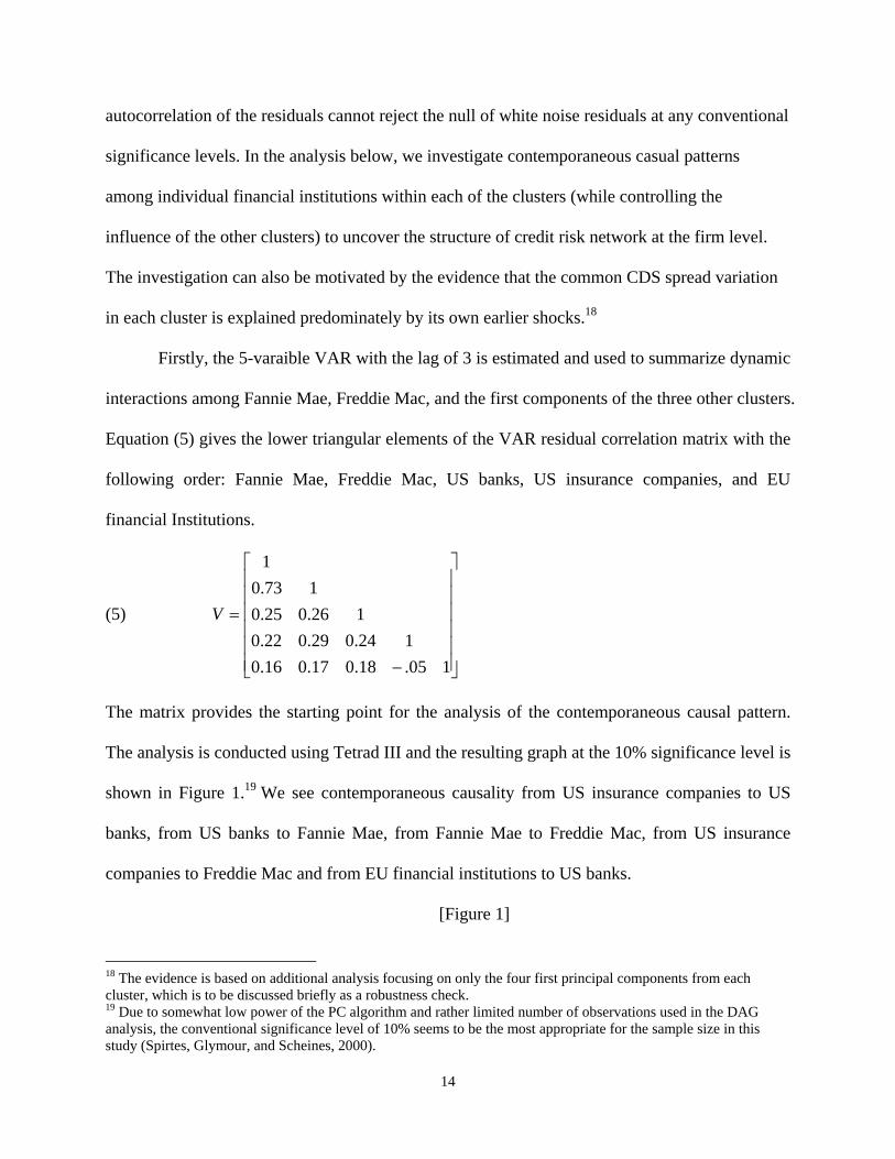
Firstly, the 5-varaible VAR with the lag of 3 is estimated and used to summarize dynamic

interactions among Fannie Mae, Freddie Mac, and the first components of the three other clusters.

Equation (5) gives the lower triangular elements of the VAR residual correlation matrix with the

following order: Fannie Mae, Freddie Mac, US banks, US insurance companies, and EU

financial Institutions.

(5)

⎥⎥⎥⎥⎥⎥

⎦

⎤

⎢⎢⎢⎢⎢⎢

⎣

⎡

−

=

105.18.017.016.0124.029.022.0

126.025.0173.0

1

V

The matrix provides the starting point for the analysis of the contemporaneous causal pattern.

The analysis is conducted using Tetrad III and the resulting graph at the 10% significance level is

shown in Figure 1.19 We see contemporaneous causality from US insurance companies to US

banks, from US banks to Fannie Mae, from Fannie Mae to Freddie Mac, from US insurance

companies to Freddie Mac and from EU financial institutions to US banks.

[Figure 1]

18 The evidence is based on additional analysis focusing on only the four first principal components from each cluster, which is to be discussed briefly as a robustness check. 19 Due to somewhat low power of the PC algorithm and rather limited number of observations used in the DAG analysis, the conventional significance level of 10% seems to be the most appropriate for the sample size in this study (Spirtes, Glymour, and Scheines, 2000).

15

As vigorously argued in Swanson and Granger (1997), the contemporaneous casual

pattern as identified through the DAG analysis of the correlation matrix provides a data-

determined solution to the basic problem of orthogonalization of VAR residuals and thus is

critical to forecast error variance decomposition of a VAR. There are two major advantages of

employing the forecast error variance decomposition: (1) allowance for time-lagged information

transmission in addition to contemporaneous information transmission; (2) description of

economic significance of dynamic causal linkages.

Based on the directed graph result in Figure 1, forecast error variance decompositions are

shown in Table 4. Entries in Table 4 give percentage of forecast error variance (standard

deviation in the table) at horizon k, which is attributable to earlier shocks (surprises) from each

other series (including itself). We list steps or horizons of 0 (contemporaneous time), 1 and 2

days (short horizon), and 10 and 30 days ahead (longer horizon). The shock to Fannie Mae very

substantially explain about 44-48% of the CDS spread variation in Freddie Mac at all horizons,

while the reverse is much weaker (about 11% at the longer horizon). Also, shocks to Fannie Mae

and Freddie Mac together can explain little of the common CDS spread variation of any other

groups, even at the longer horizon. European financial institutions have noticeable influence (6-

11%) on the credit risk of the two GSEs.

It is also interesting to note that the first principal component of the other three clusters is

explained primarily by itself both in contemporaneous time and at short horizons, with the

possible exception of the US banks, where about 10-13% of its common credit risk variations

can be explained by US insurance companies and European financial institutions. At the longer

horizon of 30 days ahead, the US insurance companies and European financial institutions

exhibit more pronounced influences on common credit risk variations of the US banks (about 8%

16

each). The European financial institutions stand out to explain about 12% of the common

variation in the CDS spreads of US insurance companies at the 30-day horizon. By contrast,

about 8% of the common credit risk variations of the European financial institutions at the 30-

day horizon can be explained by US financial institutions and particularly US banks (about 4%).

This suggests an interesting role of the European financial institutions before the global credit

crisis worsened because of the collapse of Lehman Brothers, which probably has not received

much attention. The evidence also implies that regional (or country) factors might have played

an more important role than conventionally perceived during this stage of the crisis development,

which is in line with the fact many European financial institutions had much exposure to Eastern

European economies while US financial institutions were primarily exposed to the US subprime

loan problem. In addition, different market-based assessments of probability of government

bailout for financial institutions in different countries might also factor in the change of CDS

spreads.

[Table 4]

Secondly, the 12-varaible VAR with the lag of 3 is estimated and used to summarize

dynamic interactions among 9 US banks as well as the first components of the three other

clusters. Equation (7) gives the lower triangular elements of the innovation correlation matrix

with the following order: US GSEs, US insurance companies, EU financial Institutions, Lehman

Brothers, Bear Sterns, Goldman Sachs, Merrill Lynch, Morgan Stanley, Wachovia, Citigroup,

JPMorgan, and Bank of America.

The resulting directed graph at the 10% significance level is shown in Figure 2. While no

contemporaneous relation is identified between individual US banks and the common CDS

17

spread variation of European financial institutions as a group, the interaction is channeled

through lagged credit risk transmission, as shown below in Table 5.

(7)

⎥⎥⎥⎥⎥⎥⎥⎥⎥⎥⎥⎥⎥⎥⎥⎥⎥

⎦

⎤

⎢⎢⎢⎢⎢⎢⎢⎢⎢⎢⎢⎢⎢⎢⎢⎢⎢

⎣

⎡

−

−

=

164.064.032.037.029.047.033.041.019.001.026.0156.042.041.034.059.038.048.021.002.20.0

145.033.033.044.039.047.017.012.018.0131.037.055.050.058.013.017.015.0

136.048.050.049.017.002.009.0155.035.054.009.015.015.0

165.074.022.021.027.0168.019.018.018.0

114.031.023.0105.10.0

121.01

V

From Figure 2, we can see that the individual US banks are intensively connected to one

another. Among them, Lehman Brothers appear to be a prime sender of credit risk information in

contemporaneous time, as it affects Goldman Sachs, Bear Stearns, Merrill Lynch, Citigroup, and

Wachovia, while it only receives credit risk information from Morgan Stanley (and US Insurance

as a group). Similarly, Morgan Stanley is a prime sender of credit risk information in

contemporaneous time to other banks, such as Lehman Brothers, Bank of America, and

JPMorgan, but apparently it does not receive credit risk information from any other banks (with

an undirected edge between Merrill Lynch and itself). By comparison, consistent with the role as

the exchange center of credit risk information, Goldman Sachs receive credit risk shocks in

contemporaneous time from several other investment banks, such as Lehman Brothers, Bear

Sterns, and Merrill Lynch, and also spreads out the credit risk information to GSEs and an equal

18

number of other commercial banks (i.e., Citigroup, Wachovia, and JPMorgan). Similarly, Bank

of America and Bear Sterns also appear to be the exchange center of credit risk information.

In contrast, some other commercial banks appear to be prime receivers of credit risk

information in contemporaneous time. For example, Citigroup receives credit risk information

from Lehman Brothers, Goldman Sachs, Bank of America, and Wachovia and spreads it out to

JPMorgan only. Similarly, influenced by Bear Sterns, Lehman Brothers, and Goldman Sachs,

Wachovia affects Citigroup only. The most endogenous case is JPMorgan, which is affected by

Bank of America, Citigroup, Goldman Sachs, and Morgan Stanley but has no impact on any

others in contemporaneous time.

[Figure 2 here]

The information about Goldman Sachs in Figure 2 provides more details for the edge

running from the US Banks to the US GSEs in Figure 1. Also enriching our understanding for

the edge running from US insurance companies to US banks in Figure 1, it is shown that US

insurance companies spread their common credit risk information to many other banks directly

through Lehman Brothers. Such a unique information role of Lehman Brothers would be further

collaborated and most clearly revealed in Table 5. Moreover, consistent with Figure 1, US GSEs

receive shocks from US insurance companies in the contemporaneous time, which is further

validated in the subsequent analysis (Figure 3).

Based on the directed graph result of Figure 2, forecast error variance decomposition is

also conducted and reported in Table 5. The most striking firm-level evidence is that, even with

allowance for the influence of US insurance companies and other banks, Lehman Brothers exerts

strong effects on Bear Sterns (29-33%), Goldman Sachs (35-42%), Merrill Lynch (21-26%),

Wachovia (22-27%), Citigroup (9-12%), and JPMorgan (about 10%) at all horizons. No other

19

US financial institutions under consideration have exhibited such an extensive and significant

role of credit risk information spillover, which suggests that the decision not to bail out Lehman

Brothers was probably a serious mistake and certainly worsened the global credit crisis.

Similarly, Morgan Stanley, as another prime sender of credit risk information, indeed exerts

nontrivial influence on other banks at all horizons, including Lehman Brothers (7-8%), Goldman

Sachs (5-7%), Merrill Lynch (5-8%), Citigroup (6-11%), JPMorgan (10-13%), and Bank of

America (11-12%). As an exchange center, Goldman Sachs is influenced by other four major

investment banks in contemporaneous time as 42%, 7%, 4% and 5% of its CDS spread variations

are explained by shocks to Lehman Brothers, Bear Sterns, Merrill Lynch, Morgan Stanley,

respectively. As the horizon increases, while the contributions of other investment banks largely

remain similar, shocks to two US commercial banks (i.e., JP Morgan and Bank of America)

together explain about 8% of the variation in Goldman Sachs. On the other hand, Goldman Sachs

exhibits noticeable influence and its role as the exchange center of credit risk information is

more significant at the longer horizon of 30 days ahead, explaining about 5%, 10%, and 9% of

US GSEs, Wachovia, and JPMorgan CDS variations, respectively. Consistent with the earlier

observation that JPMorgan is the most endogenous in the contemporaneous time, at a longer 30-

day horizon, it has the lowest percentage of CDS spread variations explained by its own shocks.

Lastly, consistent with Figure 1 and Table 4, US insurance companies do exert noticeable

influence on some banks. Nevertheless, even at the longer horizon, the influence of European

financial institutions on individual banks is smaller, compared to its influence on US banks as a

group in Table 4, perhaps because that the proxy used earlier only represents about 63% of the

common credit risk variation for the cluster.

[Table 5 here]

20

Thirdly, the 9-varaible VAR with the lag of 3 is estimated and used to summarize

dynamic interactions among 6 US insurance companies as well as the first components of the

other three clusters. Equation (8) gives the lower triangular elements of the innovation

correlation matrix with the following order: US GSEs, US banks, EU financial Institutions,

American Express, AIG, Chubb, Met Life, Hartford, and Safeco.

(8)

⎥⎥⎥⎥⎥⎥⎥⎥⎥⎥⎥⎥

⎦

⎤

⎢⎢⎢⎢⎢⎢⎢⎢⎢⎢⎢⎢

⎣

⎡

−−

=

174.048.064.024.029.008.20.024.0170.078.040.037.003.35.029.0

170.050.034.011.050.026.0148.034.001.040.041.0

136.020.051.031.0119.035.026.0

117.012.0119.0

1

V

The DAG analysis results in a directed graph at the 10% significance level, as shown in

Figure 3. Among US insurance companies, Safeco is a prime sender of credit risk information,

which only affects but is not affected by any other insurance companies in contemporaneous

time. A similar point can also be made for Chubb, as it receives the information only from

Safeco but send it out directly to several other insurance companies, including AIG, Met Life,

and Hartford, as well as US GSEs. AIG might also appear to be a prime sender of credit risk

information in contemporaneous time, as it affects US GSEs, US Banks, American Express, and

Met Life. Receiving the information directly from two firms (Chubb and AIG) and also sending

it out directly to US banks and Hartford, Met Life appears to be the exchange center of credit

risk information, which may also apply to American Express. By comparison, Hartford is a

prime receiver of credit risk information, as it receives the information from three other firms but

only sends it out to one firm in the contemporaneous time.

21

In Figure 3, it is revealed now that such contemporaneous causality is channeled directly

through Chubb, AIG, and American Express, which extends the finding of the edge running from

US insurance companies to US GSEs in Figure 3, Also enriching our understanding for the edge

running from US insurance companies to US banks in Figures 1-2, it is shown that US insurance

companies contemporaneously spread the common credit risk information to US banks directly

through AIG, American Express, and Met Life. European financial institutions are also

exogenous in the sense that its credit risk information directly flows to US GSEs and American

Express without inflow from others.

[Figure 4 here]

Table 6 presents results on forecast error variance decomposition based on the directed

graph result of Figure 3. Noteworthy, Chubb and Safeco are confirmed to be the prime senders of

credit risk information even at the longer horizon. Safeco has persistent and significant effect on

all other five firms in the cluster at all horizons, i.e., American Express (6-8%), AIG (8-10%),

Chubb (34-41%), Met Life (19-24%), and Hartford (41-54%), in addition to US GSEs (7-8%)

and US banks (7-10%). Chubb also exerts noticeable impacts on most of the other firms at all

horizons, including American Express (4-6%), AIG (14-15%), Met Life (22-29%), and Hartford

(16-17%), as well as US GSEs (8-9%) and US banks (9-10%). The evidence for AIG as a prime

sender of credit risk information however is weaker. Nevertheless, it still has nontrivial effects

on American Express (5%), Met Life (6%) and US banks (14%), at the longer horizon. Hartford

as a prime receiver of credit risk information is also easily confirmed as within the group it has

the lowest percentage of CDS spread variations explained by its own shocks at a longer 30-day

horizon. There is also some evidence for Met Life as the exchange center of credit risk

information, while such is more mixed for American Express. Specifically, at the short and

22

longer horizons, Met Life receives credit shocks from AIG (6%), Chubb (22-26%), and Safeco

(about 19-24%) and its shock affects Hartford (about 6-7%) and US banks (about 5%).

Moreover, consistent with the findings discussed above, European financial institutions

exhibit noticeable effects at the longer 30-day horizon. The shock to European financial

institutions as a group explains about 14%, 16%, 14%, 15%, 12%, and 6% of CDS spread

variations of American Express, AIG, Chubb, Met Life, Hartford, and Safeco, respectively.

[Table 7 here]

Finally, we estimate a 29-variable VAR with the lag of 3 for 26 European financial

institutions together with the first components of the three US clusters. Figure 4 shows

contemporaneous causal patterns based on the VAR residuals. 20 The European financial

institutions are well connected to each other and the edges are all directed (with the exception of

the edges related to the three US clusters). Noteworthy, UBS only affects but is not affected by

other institutions in the contemporaneous time, suggesting its role as a prime sender of credit risk

information. Similarly, BNP Paribs has the contemporaneous causal effects on six other

institutions (ING, Rabobank, Credit Agricole, Societe Generale, Banco Santader, and HVB)

while it is only affected by UBS. A similar point may be made for Dresdner and to a lesser extent

for Lloyds TSB. By comparison, ABN AMRO, ING, Rabobank, and Deutsche Bank may be

considered as the prime receivers of credit risk information as they only directly receive but not

send out credit risk shocks. Barclays, Commerzbank, RBS, and HVB appear to be the exchange

center of credit risk information, as they receive credit risk shocks from some firms and send out

the shock to an equal number of other firms. It is also interesting to note that Standard Chartered

20 Note that the result for this part of the analysis should be interpreted with some caution, as we are not aware of any simulation evidence on the performance of the PC algorithm applied to such a high dimensional system. Due to the same reason and further constrained by the programming capacity of the algorithm (up to 32 variables), we do not explore the potentially interesting case where all 43 financial institutions are included in one large system.

23

is the only European financial institution connected with US banks in the contemporaneous time,

although the casual relationship is undirected. Obviously, future research is needed to further

investigate the issue.

[Figure 5 here]

We also conduct the forecast error variance decomposition analysis using the estimated

VAR parameters and the orthognalized shocks based on Figure 4. To conserve the space, the

detailed decompositions are not tabulated here but are available upon request. Briefly, in the

short terms, none of the three groups of US financial institution have a significant impact on the

26 European financial institutions, consistent with the observations in Tables 4-6. At the 30-day

horizon, US GSEs explain 2.5%-7.5% of credit risk variations in some of the individual 26

institutions. By contrast, the explanatory power of US banks is typically negligible (less than

1%). The effect of US insurances on some individual European financial institutions is more

mixed and largely falls in the range of 1% and 3.5%.

5. Robustness Checks and Further Analysis

5.1. Robustness checks

We conduct many robustness checks on the main results as follows. First, the four-

variable VAR with the lag of 3 is estimated to summarize dynamic interactions among four first

principal components. It should be noted that in some cases such results based on (somewhat

imperfect) proxies of the common credit risk variation of each cluster (group) may be somewhat

different from firm-level results, which is based on richer and firm-specific information.

Nevertheless, the results based on the four first principal components (available on request),

apparently an oversimplified empirical model, is generally in line with the main findings based

on larger models using firm-level data (as reported above) (although no information on the firm-

24

level network is revealed by such an analysis). Regarding the contemporaneous causality pattern,

all directed edges are consistent with Figure 1 where the group of GSEs is the focus. One

possible exception may be the only undirected edge between US GSEs and US insurance

companies, which should be assumed to run from US insurance companies to US GSEs and

consistent with the directed edge from US insurance companies to Freddie Mac in Figure 1.

Also, the common credit risk variations of the European financial institutions as a group are

highly exogenous in the contemporaneous time, which is generally consistent with Figures 1, 3,

and 4.

The resulting error variance decomposition results confirms that every first principal

component of the four clusters is explained primarily by itself both in contemporaneous time and

at short and longer horizons, with some proportions explained by innovations in other clusters,

particularly at the longer horizon. The result generally confirms the appropriateness of the cluster

analysis result of classifying the financial institutions into 4 groups and the result in Table 4. At

30 days ahead, US banks and US insurance companies together explain about 6 percent of the

common CDS spread variation of the European financial institutions, while the European

financial institutions also have a noticeable (about 8-10%) impact on the common credit risk

variations of other groups at the longer horizon within the four clusters. The evidence is again

generally in line with Tables 4, 5, and 6, particularly in light of the fact that the first principal

component alone is an imperfect proxy even for the common variation in credit risk.

Second, we also re-estimate all the models related to US banks, US insurances and EU

financial institutions by including second principal components of each cluster (the first principal

component alone already explain 90% of the US GSEs cluster). In the main analysis above, for

the purpose of the model parsimony, we have only included the first principal component in the

25

VAR model specifications, which explains more than 60% variations for each cluster. With one

principal component for each cluster in the models, it is straightforward to interpret the results of

DAG and variance decompositions. With more than one principal component for the same

cluster included in the models, the interpretation of the empirical results is a little more

complicated. For the consideration of the simplicity, we add up the decompositions of both

principal components of the same cluster of financial institutions as the influence of the

particular cluster. The result (not reported here but available upon request) confirms that the

above finding based on the first principal components alone generally hold.

Third, we conduct a small scale simulation to assess the effectiveness of the PC algorithm

in DAG analysis in this study. Specifically, based on the estimated 12-variable VAR model of

US Banks with the lag of 3, we bootstrap a set of pseudo residuals of the same length as the

realized sample. These residuals are then used to sequentially generate a pseudo sample of CDS

spread changes for the 12 financial institutions using the estimated autoregressive parameters.

We generate a total of 100 such pseudo samples. For each sample, a VAR model with a lag

length of three is estimated. The estimated VAR residuals are retained and Tetrad III is run for

each realization using the PC algorithm and assuming causal sufficiency. Again, the chosen

significance level for DAG analysis is 10%. When there is no edge between two variables in the

true data generating process (DGPs), the PC algorithm is very successful in excluding the edge in

the simulated data, with an average success rate of 96.0%. When there is an edge, the algorithm

can both detect the existence of the edge and direct it correctly up to 60% of times. Furthermore,

it can on average correctly identify the existence of all edges in the true DGPs (i.e., the skeleton

of the causal graph) 76.3% of times (with the median success rate is 86.0%).

26

Finally, we also consider an alternative sample period. In particular, the sample contains

an unusual episode of the fall of Bear Sterns. To examine whether the inclusion of the data after

the fall of Bear Sterns has had a significant effect of the main results we have obtained, we also

re-estimate the 12-vcaraible VAR(3) for the US banks using the subsample of January 1, 2007

through –March 14, 2008 when the Bear Sterns was rescued. While the untabulated result shows

less strong evidence of credit risk network for the group of US banks due to the use of much

fewer data points, most of the main results, such as Lehman Brothers, Morgan Stanley and

Goldman Sachs as either prime senders or exchange center of credit risk information, remain

unchanged.

5.2. Driving Forces of Credit Risk Transfer

We have investigated how CDS spread changes as a proxy of credit risk transmitted

among 43 individual financial institutions. A natural question is the economic intuition for why

we would expect the spillovers to be more intense in one direction than another. Note also that

such analysis can serve as further robustness check on the above main result of the credit risk

transfer pattern, as random errors possibly introduced in the multi-step procedure (despite many

robustness checks above), if substantial, should be biased toward no significant relationship

between credit risk transfer and potential economic factors.

Toward this end, we conduct the following preliminary analysis. First, based on the

identified contemporaneous causal patterns among financial institutions, we construct an index

(called as I-index) to measure the importance of financial institutions from the perspective of

interconnectedness as follows.21 (1) Being assigned to be 3, the prime senders of credit risk

21 As discussed earlier, prime senders, exchange centers and prime receivers identified based on contemporaneous causal patterns are generally confirmed in the forecast error variance decompositions. We also conduct additional analysis to confirm the robustness of the result below. For example, when Fannie Mae is classified as a prime sender

27

information are those who send out at least two more shocks than their receipts. Specifically,

Lehman Brothers, Morgan Stanley, Sefeco, Chubb, and possibly AIG in the US and BNP Paribs,

Dresdner bank, and UBS in the Europe belong to this category. (2) The exchange centers of

credit risk information are assigned to be 2. Goldman Sachs, Bear Sterns, Bank of America, and

Metlife in the US and Barclays, RBS, Commerzbank, and HVB in the Europe play the role of the

exchange center on the credit market by intensively receiving from at least 2 financial

institutions and then transferring credit risk information to at least 2 others. (3) The prime

receivers of credit risk information are assigned to be 0, such as Citigroup, Wachovia, JPMorgan

and Hartford in the US, and ABN AMRO, ING, Rabobank, and Deutsche Bank in the Europe.

These institutions receive at least two more shocks than what they spread out. (4) The institutions

other than the above three categories are assigned to be 1. Table 8 shows the value of I-index for

each individual institution. The higher the value, the more likely an institution transfers credit

risk information to others and thus plays a more active role in the interconnected financial

network.

Second, we analyze the relationship between our I-index and various factors. Given a

small sample size with (at most) 43 observations, it is probably most appropriate to focus on the

simple regressions and 10 percent significance level (or lower). Table 9 summarizes the simple

regression results of I-index on various variables, with White’s (1980) robust standard errors.

The first factor under consideration is the size, the coefficient of which is however not

statistically significant at any conventional significance levels, regardless of using the values in

any year of 2006-08. Actually, these (insignificant) coefficient estimates are all negative. As the

financial institutions under study are all among the largest in the world, the result thus does not

instead, the results hold even better. Also, as mentioned earlier, our identification of “senders” and “receivers” of credit information is similar to primary and secondary firms in Jarrow and Fu’s (2001) model, respectively.

28

mean that the size does not matter in affecting the roles of credit risk transfer. Nevertheless, it

does imply that among the largest financial institutions, their roles of credit risk transfer may not

be related to their further somewhat differences in their sizes. Hence, from the perspective of

interconnectedness, the evidence suggests a caveat for the conventional argument of “too big to

fail.”

In contrast to size, the leverage and particularly short-term leverage ratios show their

importance in credit risk spillovers. Collin-Dufresne and Goldstein (2001) argue that a firm’s

leverage ratios have a significant impact on credit spread predictions. More relevant to this study,

both Diamond and Rajan (2009) and Acharya and Viswanathan (2011) emphasize the role of

short-term debt in affecting asset market liquidity under the crisis scenario. We employ several

leverage ratios including the ratios of total debt to total asset, short-term debt to total debt, total

debt to common equity, and short-term debt to common equity. The regression results are all

significantly positive for both debt to common equity ratios at (at least) the 10% levels across

three years of 2006-08, with short-term debt to equity ratios in 2006 and 2007 particularly

significant in predicting the cross-sectional differences in importance of credit risk transfer. The

ratio of short-term debt to total asset is also generally significant, while the ratio of total debt to

total asset is not significant in any case, perhaps because it is a noisier and less relevant measure

of the leverage to financial institutions. Thus, consistent with Collin-Dufresne and Goldstein

(2001) and particularly Diamond and Rajan (2009) and Acharya and Viswanathan (2011), the

result suggests that an institution with a higher leverage ratio and particularly a short-term

leverage ratio is more likely to transfer credit risk information to others and thus is more

important in the credit risk network from the perspective of interconnectedness. Arguably, a

financial institution with a higher leverage ratio might have more incentive to collect private

29

information about credit risk, or other financial institutions including its counterparties might

simply be more sensitive to the new information about credit risk of the more highly leverage

financial institution around the global credit crisis.

We further examine whether the roles of credit risk transfer is related to corporate

governance, as it is well documented that corporate governance may affect many aspects of

corporate performance including credit spreads (e.g., Qiu and Yu, 2009) and thus possibly credit

risk spillover. Various corporate governance measures are considered as follows: G-index is

Gompers, Ishii and Metrick’s (2003) measure of shareholders rights and E-index is Bebchuk,

Cohen and Ferrell’s (2009) measure of entrenchment, both of which are only available for US

firms. There are other corporate governance measures as follows: the board size is the total

number of directors in the firm; % independent director is the percentage of outside directors

who have no significant connection with the firm. None of these corporate governance indicators

are significant even at the 10% significant level. The result should be interpreted with caution, as

the data are only available for some firms and the sample is very small.

Another dimension of the driving forces of CDS spread change spillover might be

(il)liquidity as part of CDS spread change (albeit small) might be related to expected liquidity

premiuem (see, e.g., Bongaerts, de Jong, and Driessen, 2011). Given the data availability, we

construct two measures for illiquidity: one is the average difference between ask and bid prices

and the other is average percentage ask-bid spread normalized by the corresponding mid-quote.

The average ask-bid spread increased from 3.27 points in 2007 to 6.48 points in 2008 while the

average normalized ask-bid decreased from 20.5% in 2007 to 6.9% in 2008. However, both

measures are not statistically significant in predicting cross sectional variations of our I-index,

indicating that illiquidity might be not a major driving force of credit risk transfer among largest

30

financial institutions. Certainly, the result does not mean that the liquidity premium does not

exist on the CDS market. Nevertheless, it might not be substantial for these largest financial

institutions, which is generally consistent with the findings that the effect of liquidity is either

statistically insignificant for most widely traded CDS spreads (Acharya and Johnson, 2007) or

statistically significant but economically small even for a large cross-section of CDS spreads

(Bongaerts, de Jong, and Driessen, 2011).

Finally, we conduct the analysis on how asset write-downs by financial institutions might

affect the roles of credit risk transfer. From the Bloomberg, the absolute values of write-down 22

and the percentage values normalized by total asset and/or market value are potentially direct

measures of how hard an institution was hit in the credit crunch and could be to some extent

proxies for counter party risk as discussed in Jorion and Zhang (2009). However, as shown in

Table 9, the results are all insignificant. The result, while it could be due to the relatively small

sample, may be consistent with the observation that write-down more likely reflects

opportunistic reporting by managers rather than the provision of their private information (Riedl,

2004) or that financial contagion was not propagated through a correlated-information channel

(Longstaff, 2010). The above analysis is obviously preliminary, and further research is needed to

examine the issue in more depth.

6. Conclusions

This study uses credit default spreads to sort out the structure of credit risk spillovers

among the 43 largest international financial institutions around the recent global credit crisis. We

propose and apply a relatively novel empirical framework that combines cluster analysis,

principle component analysis, and DAG-based VAR analysis. Using hierarchical cluster analysis, 22 The total magnitude of losses in all firms covered by Bloomberg is about US $1,000 billion for our sample period. Bloomberg collects write downs by quarter and also classifies them into various groups based on company disclosure. For simplicity, we aggregate write downs by year for each financial institution.

31

we classify financial institutions into four clusters based on their credit risk: US GSEs, US banks,

US insurance companies, and European financial institutions. The first component in each cluster

is also found to be the major driving force, explaining more than 60% of total variation.

To investigate the structure of credit risk spillover at the firm level, we consider

interactions among individual financial institutions within a particular cluster while controlling

for the influence of the other clusters. We are able to identify three groups of players including

prime senders, exchange centers and prime receivers of credit risk information. Noticeably,

before its collapse, Lehman Brothers already surpassed all other US banks under consideration to

exert a pervasive impact on credit risk of US banks. Credit risk shocks to European financial

institutions as a group often has a noticeable impact on individual US GSEs and US insurance

companies, but not on individual US banks, even at the longer horizon. The main findings are

quite reliable based on the simulation evidence and generally robust against alternative model

specifications and sample periods. Further analysis shows that consistent with the literature (e.g.,

Acharya and Viswanathan, 2011; Collin-Dufresne and Goldstein, 2001; Diamond and Rajan,

2009), leverage ratios and particularly short-term debt ratios appear to be significant

determinants of identified different roles of financial institutions in credit risk transfer. There is

little preliminary evidence that other factors including corporate governance indexes, size,

liquidity and write-downs can explain the cross-sectional differences of the credit risk transfer

roles among these financial institutions, which is also consistent with many earlier works (e.g.,

Acharya and Johnson, 2007; Bongaerts, de Jong, and Driessen, 2011; Riedl, 2004).

The findings of this study provide considerable information to policymakers, as they shed

light on the structure of the credit risk network among financial institutions and the identification

of SIFIs from the perspective of interconnectedness with the focus on credit risk. The current key

32

policy initiative to address the SIFIs is to use a basket of measures to identify these SIFIs and

impose additional capital surcharge of 1% to 2.5% of risk-weighted assets. Our findings also

offer more specific implications for regulation, suggesting that capital surcharge should be

particularly based on short-term debt ratio. Further research may be fruitful to more thoroughly

examine different firm characteristics and different channels affecting the role of individual

financial institutions in credit risk transfer (e.g., Beltratti and Stulz, 2010).

33

References

Acharya, V.V., Perdersen, L.H., Philippon, T., Richarson, M. (2010), “Measuring Systemic

Risk,” Working Paper, New York University.

Acharya, V.V., Viswanathan, S., (2011). “Leverage, Moral Hazard and Liquidity,” Journal of

Finance, 66, 99-138.

Acharya, V.V., Johnson, T., (2007) “Insider Trading in Credit Derivatives,” Journal of Financial

Economics, 84, 110-141.

Adrian, T, Brunnermeier, M.K. (2009), “CoVAR,” Working Paper, University of Princeton.

Allen, F., Babus, A., Carletti, E. (2009), “Financial Connections and Systemic Risk,” Working

Paper, University of Pennsylvania.

Allen, F., Carletti, E., (2006). “Credit risk transfer and contagion,” Journal of Monetary

Economics, 53, 89-111.

Bae, K-H, Karolyi, G.A., and Stulz, R.M. (2003), “A New Approach to Measuring Financial

Contagion,” Review of Financial Studies, 16, 717-763.

Bebchuk, L., Cohen, A., Ferrell, A. (2009), “What Matters in Corporate Governance,” Review of

Financial Studies, 22, 783-827

Beltratti, A., Stulz, R.M., (2010). “The credit crisis around the globe: Why did some banks

perform better?” Working Paper, Ohio State University.

Blanco, R. Brennan, S., and March, I.W.(2005). “An Empirical Analysis of the Dynamic

Relationship Between Investment-Grade Bonds and Credit Default Swaps,” Journal of

Finance, 60, 2255-2281.

Bongaerts, D., F. de Jong, and J. Driessen, (2011). “Derivative Pricing with Liquidity Risk: Theory

and Evidence from the Credit Default Swap Market.” Journal of Finance, 66, 203-240.

34

Brunnermeier, M.K. (2009), “Deciphering the Liquidity and Credit Crunch 2007-2008,” Journal

of Economic Perspectives, 23, 77-100.

Collin-Dufresne, P., and Goldstein, B. (2001). “Do credit spreads reflect stationary leverage

ratios.” Journal of Finance, 56, 2177–208.

Cossin, D., Schellhorn, H., (2007). “Credit Risk in a Network Economy,” Management Science,

53, 1604-1617.

Diamond, D. W., Rajan, R.G. (2009). “The Credit Crisis: Conjectures about Causes and

Remedies,” American Economic Review Papers and Proceedings, 99, 606-610.

Eichengreen, B., Mody, A., Nedljkovic, M., and Sarno, L. (2009), “How the Subprime Crisis

Went Global: Evidence from Bank Credit Default Swap Spreads,” NBER working paper

14904.

Elsinger, H., Lehar, A., and Summer, M. (2006). “Risk Assessment for Banking Systems.”

Management Science, 52, 1301–1314.

Ericsson, J., Jacobs, K., and Oviedo, R. (2009), “The determinants of credit default swap

premia,” Journal of Financial and Quantitative Analysis, 44, 109-132.

Eun, C., Shim, S. (1989), “International transmission of stock market movements,” Journal of

Financial and Quantitative Analysis, 24, 241-256.

Forbes, K. J., Rigobon, R.(2002) “No contagion, only interdependence: measuring stock market

comovements,” Journal of Finance, 57, 2223-2261.

Gagnon, L., Karolyi, G.A., (2009). “Information, Trading Volume, and International Stock

Return Comovements: Evidence from Cross-listed Stocks”, Journal of Financial and

Quantitative Analysis, 44, 953-986.

35

Gompers, P., Ishii, J. Metrick, A. (2003). “Corporate Governance and Equity Prices,” Quarterly

Journal of Economics, 116, 107-155

Hoover, K.D., (2005). “Automatic inference of the contemporaneous causal order of a system of

equations.” Econometric Theory, 21, 69-77.

Huang, X., Zhou, H., Zhu, H.(2009), “A Framework for assessing the Systematic Risk of Major

Financial Institutions,” Journal of Banking and Finance, 33, 2036-2049.

Jarrow, R., Yu, F. (2001) “Counterparty Risk and the Pricing of Defaultable Securities.” Journal

of Finance, 56, 1765-1799.

Jorion, P., Zhang, G. (2007). “Good and bad credit contagion: Evidence from credit

default swaps,” Journal of Financial Economics, 84, 860-883.

Jorion, P., Zhang, G., (2009). “Credit Contagion from Counterparty Risk.” Journal of Finance,

64, 2053-2087.

Li, H., Zhang, W., and Kim, G. (2011). “The CDS-Bond Basis and the Cross Section of

Corporate Bond Returns.” Working paper, University of Michigan and National

University of Singapore.

Leuz, C., Nanda, D. and Wysocki, P.D. (2003). “Earnings management and investor protection:

An international comparison.” Journal of Financial Economics, 69, 505-527.

Longstaff, F.A., (2010). “The Subprime Credit Crisis and Contagion in Financial Markets,”

Journal of Financial Economics, 97, 436-450.

Longstaff, F.A., Mithdal, S. and Nies, E. (2005), “Corporate Yield Spreads: Default Risk or

Liquidity? New Evidence from the Credit-Default-Swap Market,” Journal of Finance, 60,

2213-2253.

Ludvigson, S. C., and S. Ng. (2009). “Macro factors in bond risk premia.” Review of Financial

36

Studies, 22, 5027-5067.

Pearl, J., (2000). Causality: Models, Reasoning, and Inference. Cambridge University Press,

Cambridge.

Qiu, J., Yu, F. (2009). “The market for corporate control and the cost of debt,” Journal of

Financial Economics, 93, 505-524.

Riedl, E.,(2004). “An examination of long-lived asset impairments,” The Accounting Review, 79,

823-852.

Sims, C., (1980). “Macroeconomics and reality.” Econometrica, 48, 1-48.

Spirtes, P., Glymour, C., Scheines, R. (2000), Causation, Prediction, and Search. MIT Press,

Cambridge.

Stulz, R.M., (2010). “Credit Default Swaps and the Credit Crisis,” Journal of Economic

Perspectives, 24 (Winter), 73-92.

Swanson, N., Granger, C.W.J. (1997), “Impulse response functions based on a causal approach

to residual orthogonalization in vector autoregression,” Journal of the American

Statistical Association, 92, 357-367.

White, H., (1980). “A heteroscedasticity-consistent covariance matrix estimator and a direct test

for heteroscedasticity.” Econometrica, 48, 817-838.

Zhang, B., Zhou, H., and Zhu, H. (2009), “Explaining credit default swap spreads with the equity

volatility and jump risks of individual firms,” Review of Financial Studies 22, 5099-5131.

37

Table 1: Summary statistics of CDS Spreads

This table reports summary statistics on CDS spreads for 43 financial institutions from January 1, 2007 to September 9, 2008. The means, standard deviations, minimum and maximum values are based on mid-quotes. The ask-bid are differences between ask and bid prices and the normalized ask-bid is the ask-bid divided by the corresponding mid-quote.

Country Name Mean Std. Dev. Min Max Average

Ask-bid

Average normalized

ask-bid US Fannie Mae 32.22 21.83 6.40 87.58 2.53 0.11 US Freddie Mac 32.09 22.06 5.25 88.15 2.74 0.12 US Lehman Brothers 139.16 103.80 20.81 425.14 6.01 0.06 US Bearn Sterns 114.66 96.36 20.83 727.14 5.54 0.06 US Goldman Sachs 77.69 47.16 20.90 244.44 4.25 0.07 US Merrill Lynch 123.28 94.52 15.63 342.19 5.47 0.07 US Morgan Stanley 103.52 73.09 17.83 297.30 5.31 0.07 US Bank of America 54.60 39.33 8.68 147.25 4.17 0.13 US Wachovia 97.94 90.68 11.10 358.51 4.35 0.14 US Citigroup 70.45 57.51 7.44 226.60 4.58 0.14 US JP Morgan 55.72 35.23 14.49 163.83 3.73 0.09 US Met Life 66.11 60.01 11.00 240.59 4.34 0.11 US Safeco 43.33 26.64 17.90 135.03 4.41 0.13 US American express 86.26 75.36 8.91 250.67 5.94 0.13 US AIG 96.04 96.93 8.93 446.24 5.63 0.14 US Chubb 38.72 27.42 9.86 125.92 3.65 0.13 US Hartford 62.14 61.54 10.72 293.26 4.47 0.12 UK Abbey 44.75 35.84 4.33 155.56 4.17 0.21 UK Barclays 52.83 43.50 5.45 173.00 4.31 0.17 UK HBOS 70.83 66.28 4.77 253.10 6.95 0.15 UK HSBC 39.01 30.67 4.94 155.00 4.18 0.22 UK Lloyds TSB 37.46 31.62 3.67 135.81 3.82 0.26 UK RBS 52.95 43.56 4.06 204.94 4.20 0.17 UK Standard Chartered 43.79 31.96 5.63 139.88 5.44 0.25 France AXA 56.50 43.55 9.10 197.75 4.94 0.15 France BNP Paribas 33.59 25.00 5.7 119.59 3.68 0.18 France Credit Agricole 45.11 37.19 5.84 161.82 4.64 0.17 France Societe Generale 42.53 34.73 6.01 148.60 4.28 0.20 Germany Allianz 41.10 29.25 6.04 133.02 4.33 0.18 Germany Commerzbank 49.39 34.58 8.16 164.50 4.69 0.15 Germany HVB 42.62 30.69 6.17 144.81 4.53 0.19 Germany Deutsche Bank 47.49 32.20 9.82 155.13 4.54 0.14 Germany Dresdner Bank 49.83 39.84 5.48 167.85 4.77 0.20 Germany Hannover Rueckversicherung 41.64 29.57 8.50 143.93 4.34 0.16 Italy Banco Monte Dei Paschi 44.31 32.69 6.13 158.07 7.37 0.17 Italy UniCredit SpA 43.03 29.26 7.48 151.42 4.07 0.14 Netherlands ABN AMRO 48.39 39.32 5.53 189.22 4.18 0.16 Netherlands ING 44.84 39.80 4.62 177.49 4.22 0.21 Netherlands Rabobank 28.86 24.47 3.00 99.83 3.52 0.26 Switzerland Credit Suisse 52.24 37.72 9.86 186.26 4.42 0.12 Switzerland UBS 53.97 48.12 4.55 225.25 4.73 0.2 Spain Banco Santader 45.39 33.66 7.62 152.39 4.34 0.16 Portugal Banco Commercial Portugues 48.58 34.99 8.15 157.21 4.48 0.15

38

Table 2: Cluster Analysis This table reports 4 clusters of 43 largest financial institutions based on a hierarchical cluster analysis. The average linkage method is used to measure the distance between cluster pairs and the cubic cluster criterion (CCC) is used to choose the number of clusters. Cluster 1 (US GSEs)

Cluster 2 (US Banks)

Cluster 3 (US Insurances)

Cluster 4 (EU Financial Institutions)

Fannie Mae Lehman Brothers Met Life Abbey Freddie Mac Bearn Sterns Safeco Barclays Goldman Sachs American express HBOS Merrill Lynch AIG HSBC Morgan Stanley Chubb Lloyds TSB Bank of America Hartford RBS Wachovia Standard Chartered Citigroup AXA JP Morgan BNP Paribas Credit Agricole Societe Generale Allianz Commerzbank HVB Deutsche Bank Dresdner Bank Hannover Rueckversicherung Banco Monte Dei Paschi UniCredit SpA ABN AMRO ING Rabobank Credit Suisse UBS Banco Santader Banco Commercial Portugues

39

Table 3: Principal Component Analysis

This table reports the cumulative fractions of the total variation explained by the first few principal components in each cluster. The clusters are defined as in Table 2. The cumulative fractions are computed as the ratio between the sum of the first few largest eigenvalues divided by the sum of all eigenvalues. Cluster 1

(US GSEs) Cluster 2 (US Banks)

Cluster 3 (US Insurances)

Cluster 4 (EU Financial Institutions)

1st factor 90.04% 62.56% 66.13% 70.82% First 2 factors 100% 72.32% 80.23% 80.17% First 3 factors 79.24% 89.44% 82.50% First 4 factors 85.27% 94.14% 84.52% First 5 factors 89.54% 97.49% 86.49%

40

Table 4: Forecast error variance decomposition results (percentage) among US GSEs and the other three clusters

Day Fannie Mae Freddie Mac US Banks

US Insurances

EU financial institution

Variance of Fannie Mae explained by shocks to the five CDS spreads 0 93.7 0.0 5.7 0.4 0.2 1 84.7 8.1 5.1 0.7 1.4 2 81.0 10.9 4.9 1.0 2.2 10 76.2 11.0 5.1 1.7 6.1 30 76.1 11.0 5.1 1.7 6.1

Variance of Freddie Mac explained by shocks to the five CDS spreads 0 47.7 45.9 2.9 3.4 0.1 1 48.9 44.2 3.3 2.6 0.9 2 47.0 41.5 3.8 3.6 4.1 10 43.9 38.0 3.9 3.9 10.3 30 43.9 38.0 4.0 3.9 10.3

Variance of US banks explained by shocks to the five CDS spreads 0 0.0 0.0 90.1 6.3 3.7 1 0.0 0.4 86.3 8.3 5.0 2 0.3 0.3 84.4 8.1 6.9 10 0.9 0.8 81.4 8.9 8.0 30 0.9 0.8 81.3 8.9 8.1

Variance of US insurances explained by shocks to the five CDS spreads 0 0.0 0.0 0.0 100.0 0.0 1 0.0 0.6 0.0 99.4 0.0 2 0.0 0.9 0.2 97.6 1.2 10 0.2 1.0 1.1 86.3 11.5 30 0.2 1.0 1.1 86.2 11.5

Variance of EU financial institutions explained by shocks to the five CDS spreads 0 0.0 0.0 0.0 0.0 100.0 1 0.1 0.1 0.5 0.9 98.3 2 0.3 0.4 2.3 1.8 95.4 10 1.3 0.5 3.9 1.9 92.4 30 1.3 0.5 3.9 1.9 92.4

Note: The variance decomposition is based on the directed graph on innovations given in Figure 1.

41

Table 5: Forecast error variance decomposition results (percentage) for US banks and first principle components of other groups

Days US GSEs

US Insurances

EU financial

Institutions

LehmanBrothers

Bear Sterns

GoldmanSachs

Merrill Lynch

MorganStanley Wachovia Citi-

groupJP

MorganBank of America

Variance of US GSEs explained by the shocks of the 12 CDS spreads 0 90.1 4.6 0.0 2.4 0.4 2.1 0.2 0.3 0.0 0.0 0.0 0.0 1 83.6 4.5 0.0 3.0 0.5 3.5 0.2 1.9 0.7 1.9 0.2 0.1 2 76.2 4.3 1.7 3.8 1.3 4.6 0.6 2.7 0.6 3.3 1.0 0.1 30 67.6 4.1 5.7 3.6 1.9 5.3 0.9 4.1 2.0 3.1 1.2 0.4

Variance of US insurances explained by the shocks of the 12 CDS spreads 0 0.0 100 0.0 0.0 0.0 0.0 0.0 0.0 0.0 0.0 0.0 0.0 1 0.3 96.8 0.0 0.1 0.0 0.0 0.0 0.0 0.4 0.5 1.8 0.0 2 0.4 91.3 0.4 0.1 2.6 0.0 0.5 0.3 0.5 0.6 3.4 0.1 30 0.5 77.3 7.0 0.5 4.2 1.5 1.0 1.1 2.1 0.9 3.3 0.8

Variance of EU financial institutions explained by the shocks of the 12 CDS spreads 0 0.0 0.0 100 0.0 0.0 0.0 0.0 0.0 0.0 0.0 0.0 0.0 1 0.0 0.8 94.5 0.1 0.1 1.1 0.2 1.6 0.1 0.5 0.7 0.4 2 0.1 1.4 85.8 0.6 0.1 3.6 0.2 5.0 0.2 0.7 0.8 1.5 30 0.3 1.9 77.1 1.8 0.9 7.0 0.9 5.9 0.4 0.7 1.0 2.3

Variance of Lehman Brothers explained by the shocks of the 12 CDS spreads 0 0.0 10.7 0.0 80.9 0.7 0.0 0.1 7.8 0.0 0.0 0.0 0.0 1 0.5 10.1 0.0 77.2 0.7 0.2 0.4 8.0 0.2 0.2 1.3 1.5 2 0.9 9.9 1.1 71.8 0.6 1.2 0.9 7.5 0.3 0.3 2.3 3.4 30 0.9 9.0 3.5 67.6 0.7 2.6 1.4 7.5 0.3 0.4 2.5 3.8

Variance of Bear Sterns explained by the shocks of the 12 CDS spreads 0 0.0 4.1 0.0 31.1 61.8 0.0 0.1 2.9 0.0 0.0 0.0 0.0 1 0.4 6.2 0.6 32.6 54.2 0.0 0.1 2.4 0.4 0.0 1.7 1.5 2 0.4 6.3 2.9 30.9 50.7 0.2 0.1 2.4 0.6 0.1 2.9 2.6 30 0.6 6.3 4.5 28.7 46.4 2.4 1.2 3.2 0.6 0.6 2.7 3.0

42

Table 5 (Continued)

Days US GSEs

US Insurances

EU financial

Institutions

LehmanBrothers

Bear Sterns

GoldmanSachs

Merrill Lynch

MorganStanley Wachovia Citi-

groupJP

MorganBank of America

Variance of Goldman Sachs explained by the shocks of the 12 CDS spreads 0 0.0 5.6 0.0 42.2 7.0 37.2 3.5 4.6 0.0 0.0 0.0 0.0 1 0.3 6.6 0.0 39.5 6.7 33.1 2.2 6.5 0.2 1.1 1.2 2.8 2 0.4 6.3 0.5 36.7 6.2 31.3 3.0 6.5 0.2 1.6 2.5 4.8 30 0.5 6.2 1.6 35.4 5.9 30.7 3.1 6.7 0.4 1.7 3.3 4.8

Variance of Merrill Lynch explained by the shocks of the 12 CDS spreads 0 0.0 2.8 0.0 20.8 0.4 0.0 76.5 4.7 0.0 0.0 0.0 0.0 1 0.0 4.0 0.5 25.7 0.3 0.8 54.8 8.2 0.0 1.0 1.9 2.8 2 0.1 3.6 1.0 21.6 0.3 2.5 52.7 7.5 0.0 1.8 3.7 5.3 30 0.2 3.8 1.3 20.5 0.7 3.6 51.0 7.4 0.3 2.0 4.0 5.5

Variance of Morgan Stanley explained by the shocks of the 12 CDS spreads 0 0.0 0.7 0.0 4.8 7.0 0.0 0.7 86.9 0.0 0.0 0.0 0.0 1 0.7 3.7 0.2 7.0 7.5 0.1 1.0 76.6 0.9 0.0 2.0 0.1 2 1.0 4.9 1.7 7.5 6.9 0.3 0.9 70.8 0.9 0.1 4.4 0.9 30 1.0 5.6 2.3 7.5 6.7 0.9 1.6 67.5 0.9 0.2 4.5 1.4

Variance of Wachovia explained by the shocks of the 12 CDS spreads 0 0.0 3.5 0.0 26.4 3.8 1.9 0.2 2.6 61.7 0.0 0.0 0.0 1 0.3 2.3 0.0 26.8 6.0 6.5 0.2 4.1 50.7 0.1 0.3 2.9 2 1.1 2.3 0.1 24.6 5.8 6.9 0.8 3.8 45.9 0.2 0.6 8.2 30 1.4 2.1 0.5 22.4 5.4 9.8 1.0 3.9 43.7 0.5 1.1 8.4

Variance of Citigroup explained by the shocks of the 12 CDS spreads 0 1.4 1.6 0.0 8.5 1.0 0.0 0.1 6.4 3.1 54.2 0.0 23.9 1 2.8 1.2 1.7 11.1 0.8 0.2 0.4 11.7 2.7 42.5 0.3 24.8 2 3.4 2.9 3.0 11.8 1.1 0.3 0.8 11.3 2.6 38.3 1.1 23.6 30 3.5 4.6 3.5 11.8 1.1 0.8 1.2 10.9 3.1 35.8 1.4 22.3

43

Table 5 (Continued)

Days US GSEs

US Insurances

EU financial

Institutions

LehmanBrothers

Bear Sterns

GoldmanSachs

Merrill Lynch

MorganStanley Wachovia Citi-

groupJP

MorganBank of America

Variance of J.P. Morgan explained by the shocks of the 12 CDS spreads 0 1.0 1.8 0.0 10.3 2.7 4.6 0.7 9.7 0.1 1.6 50.3 17.4 1 1.4 2.4 2.9 9.7 2.5 3.4 0.5 12.9 0.1 1.9 34.8 27.8 2 2.0 2.5 4.5 10.5 2.9 4.3 0.8 12.5 0.1 1.7 32.3 25.9 30 2.4 3.4 4.7 10.0 3.2 8.5 1.5 12.2 0.1 1.6 28.9 23.8

Variance of Bank of America explained by the shocks of the 12 CDS spreads 0 4.8 0.6 0.0 1.3 1.1 0.1 0.2 11.1 0.0 0.0 0.0 80.9 1 4.9 0.7 0.9 5.0 1.4 0.1 0.8 12.4 0.0 0.3 0.5 73.3 2 4.7 3.0 1.9 6.9 2.2 0.2 1.7 11.1 0.0 0.6 2.5 65.2 30 5.0 4.2 2.8 7.1 2.2 1.9 1.9 10.8 0.5 0.7 3.1 60.1

Note: The variance decomposition is based on the directed graph on innovations given in Figure 2. The values are the averages of two different assumed edges for the only undirected edge between Morgan Stanley and Merrill Lynch.

44

Table 6: Forecast error variance decomposition results (percentage)

for US insurance companies and first principle components of other groups

Days US GSEs

US Banks

EU financialInstitutions

AmericanExpress AIG Chubb Met Life Hartford Safeco

Variance of US GSEs explained by shocks to the nine CDS spreads 0 80.6 0.0 0.9 0.7 1.3 9.4 0.0 0.0 7.0 1 76.3 0.2 2.1 2.6 2.2 8.4 0.1 0.0 8.0 2 71.3 1.1 5.0 3.1 2.8 8.0 0.2 0.9 7.6 30 64.3 1.3 8.5 3.5 4.1 7.9 0.5 2.7 7.1

Variance of US Banks explained by shocks to the nine CDS spreads 0 0.0 65.4 0.0 1.4 12.6 9.0 4.5 0.0 7.0 1 0.4 59.1 0.3 1.6 14.3 9.6 5.1 0.0 9.5 2 0.5 57.6 2.7 1.8 13.9 9.3 4.9 0.1 9.2 30 0.8 52.3 5.2 2.9 13.5 10.1 4.9 0.3 9.9

Variance of EU financial institutions explained by shocks to the nine CDS spreads 0 0.0 0.0 100 0.0 0.0 0.0 0.0 0.0 0.0 1 0.1 0.1 96.9 0.0 2.0 0.1 0.2 0.3 0.3 2 0.4 0.9 93.8 0.0 2.9 0.2 0.3 0.7 0.9 30 1.2 2.4 87.9 0.3 3.1 1.3 0.9 2.2 0.8

Variance of American Express explained by shocks to the nine CDS spreads 0 0.0 0.0 2.4 79.3 4.1 3.9 0.3 2.2 7.7 1 0.0 0.3 8.1 72.6 5.3 5.6 0.5 1.5 6.0 2 0.0 0.3 12.9 68.9 4.9 5.1 0.5 1.4 6.1 30 1.0 0.7 14.3 64.6 4.9 6.0 0.8 1.5 6.3

Variance of AIG explained by shocks to the nine CDS spreads 0 0.0 0.0 0.0 0.0 76.7 13.8 0.0 0.0 9.5 1 0.0 0.0 2.5 1.2 71.6 14.9 0.6 0.1 9.1 2 0.1 0.2 10.7 2.5 63.2 14.1 0.8 0.2 8.1 30 1.6 0.8 16.4 2.4 54.7 15.0 1.0 0.3 7.8

45

Table 6 (Continued)

Days US GSEs

US Banks

EU financialInstitutions

AmericanExpress AIG Chubb Met Life Hartford Safeco

Variance of Chubb explained by shocks to the nine CDS spreads 0 0.0 0.0 0.0 0.0 0.0 59.4 0.0 0.0 40.6 1 0.4 0.2 0.2 0.9 0.6 55.0 0.4 0.0 42.3 2 0.6 0.2 3.3 1.2 1.4 52.7 0.4 0.2 40.1 30 0.8 0.5 13.6 1.4 1.9 46.7 1.0 0.5 33.5

Variance of Met Life explained by shocks to the nine CDS spreads 0 0.0 0.0 0.0 0.0 3.5 28.9 47.8 0.0 19.8 1 0.0 0.2 0.4 0.2 6.4 26.4 41.8 0.3 24.4 2 0.0 0.2 6.3 0.4 6.7 24.0 38.4 1.4 22.6 30 0.4 1.0 14.9 0.6 6.4 21.9 34.1 1.9 18.9

Variance of Hartford explained by shocks to the nine CDS spreads 0 0.0 0.0 0.0 0.0 0.3 16.7 3.6 25.9 53.6 1 0.4 0.0 0.3 0.8 1.7 16.9 5.9 21.7 52.3 2 0.4 0.0 3.1 0.8 3.4 16.1 5.7 20.6 49.9 30 0.8 0.3 12.1 1.4 3.3 15.8 6.8 18.1 41.3

Variance of Safeco explained by shocks to the nine CDS spreads 0 0.0 0.0 0.0 0.0 0.0 0.0 0.0 0.0 100 1 1.4 0.1 0.0 0.1 0.5 0.3 0.7 0.2 96.7 2 1.8 0.1 0.6 0.7 1.3 0.7 0.9 0.8 93.1 30 1.8 0.4 5.8 2.0 1.4 1.7 2.1 2.0 82.8

Note: The variance decomposition is based on the directed graph on innovations given in Figure 3.

46

Table 7: I-index This table reports I-index (importance index from the perspective of interconnectedness) for 43 financial institutions based on their contemporaneous causal patterns. Assigned to be 3, the prime senders of credit risk information are those who send out at least two more shocks than what their receive. Assigned to be 0, the prime receivers of credit risk information are institutions which receive at least two more shocks than what they spread out. The exchange centers of credit risk information are assigned to be 2. They intensively receive from at least 2 financial institutions and then transfer credit risk information to at least 2 others. The institutions other than the above three categories are assigned to be 1.

Country Name I-indexUS Fannie Mae 1 US Freddie Mac 1 US Lehman Brothers 3 US Bearn Sterns 2 US Goldman Sachs 2 US Merrill Lynch 1 US Morgan Stanley 3 US Bank of America 2 US Wachovia 0 US Citigroup 0 US JP Morgan 0 US Met Life 2 US Safeco 3 US American express 1 US AIG 3 US Chubb 3 US Hartford 0 UK Abbey 1 UK Barclays 2 UK HBOS 1 UK HSBC 1 UK Lloyds TSB 1 UK RBS 2 UK Standard Chartered 1 France AXA 1 France BNP Paribas 3 France Credit Agricole 1 France Societe Generale 1 Germany Allianz 1 Germany Commerzbank 2 Germany HVB 2 Germany Deutsche Bank 0 Germany Dresdner Bank 3 Germany Hannover Rueckversicherung 1 Italy Banco Monte Dei Paschi 1 Italy UniCredit SpA 1 Netherlands ABN AMRO 0 Netherlands ING 0 Netherlands Rabobank 0 Switzerland Credit Suisse 1 Switzerland UBS 3 Spain Banco Santader 1 Portugal Banco Commercial Portugues 1

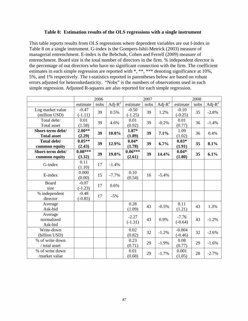
47

Table 8: Estimation results of the OLS regressions with a single instrument This table reports results from OLS regressions where dependent variables are out I-index in Table 8 on a single instrument. G-index is the Gompers-Ishii-Metrick (2003) measure of managerial entrenchment. E-index is the Bebchuk, Cohen and Ferrell (2009) measure of entrenchment. Board size is the total number of directors in the firm. % independent director is the percentage of out directors who have no significant connection with the firm. The coefficient estimates in each simple regression are reported with *, **, *** denoting significance at 10%, 5%, and 1% respectively. The t-statistics reported in parentheses below are based on robust errors adjusted for heteroskedasticity. “Nobs” is the numbers of observations used in each simple regression. Adjusted R-squares are also reported for each simple regression.

2006 2007 2008 estimate nobs Adj-R2 estimate nobs Adj-R2 estimate nobs Adj-R2

Log market value (million USD)

-0.47 (-1.11) 39 0.5% -0.50

(-1.25) 39 1.2% -0.10 (-0.25) 35 -2.8%

Total debt/ Total asset

0.01 (1.58) 39 4.6% 0.01

(0.92) 39 -0.2% 0.01 (0.77) 36 -1.4%

Short-term debt/ Total asset

2.00** (2.29) 39 10.8% 1.87*

(1.89) 39 7.1% 1.09 (1.02) 36 0.4%

Total debt/ common equity

0.05** (2.43) 39 12.9% 0.04*

(1.78) 39 6.7% 0.03* (1.91) 35 8.1%

Short-term debt/ common equity

0.08*** (3.32) 39 19.8% 0.06***

(2.61) 39 14.4% 0.04* (1.80) 35 6.1%

G-index 0.11 (1.10) 17 -1.4%

E-index 0.000 (0.00) 15 -7.7% 0.10

(0.54) 16 -5.4%

Board size

-0.07 (-1.23) 17 0.6%

% independent director

-0.48 (-0.85) 17 -5%

Average Ask-bid 0.28

(1.09) 43 -0.5% 0.11 (1.21) 43 1.3%

Average normalized

Ask-bid -2.27

(-1.31) 43 0.9% -7.76 (-0.64) 43 -1.2%

Write-down (billion USD) 0.02

(0.82) 32 -1.2% -0.004 (-0.46) 32 -2.6%

% of write down / total asset 0.23

(0.71) 29 -1.9% 0.08 (0.77) 29 -1.6%

% of write down /market value 0.01

(0.68) 29 -1.7% 0.001 (1.05) 28 -2.7%

48

Figure 1 Contemporaneous causal flow patterns among US GSEs and other clusters

EU financial Institutions

US Banks

Fannie Mae US Insurances

Freddie Mac

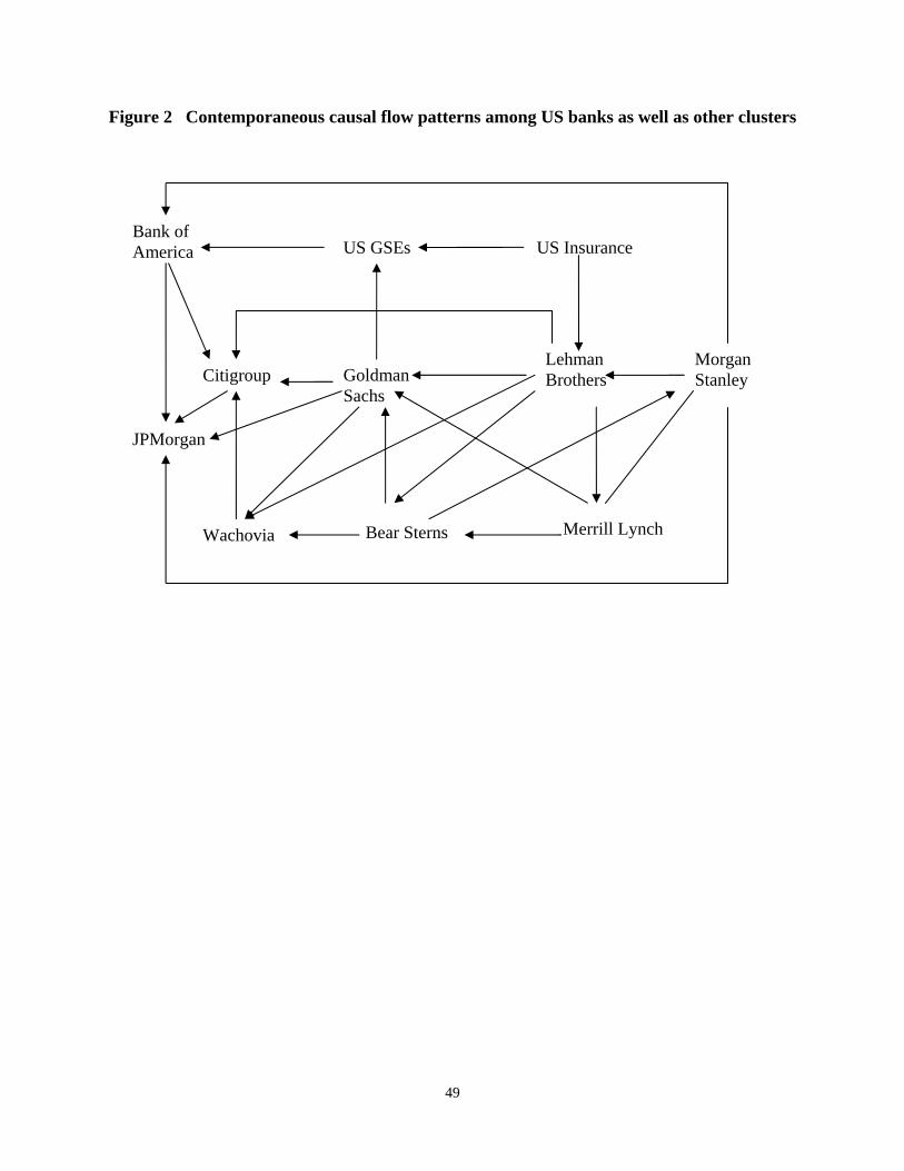
49

Figure 2 Contemporaneous causal flow patterns among US banks as well as other clusters

US Insurance Bank of America US GSEs

Goldman Sachs

Lehman Brothers Citigroup

Merrill Lynch Bear Sterns Wachovia

Morgan Stanley

JPMorgan

50

Figure 3 Contemporaneous causal flow patterns among US insurance companies as well as other clusters

EU financial Institutions

US GSEs

AIG US BanksChubb

Met LifeHartfordSafeco

American Express

51

Figure 4 Contemporaneous casual flow patterns among European financial institutions as well as other clusters

Societe Generale

Credit Agricole

Hannover Rueckversicherung

ING HSBC

Banco Santader

BNP Paribas Robo-

bank

Lloyds TSB

ABN AMRO

Banco Monte Dei Paschi

Deutsche Bank

HVB Barclays Abbey AXA

Dresdner Bank

UBS RBS HBOs

UniCredit SpA

Credit Suisse

Commerzbank Allianz Banco Commercial Portugues

Standard Chartered

US banks

US Insurances

US GSEs