1

Cross-Border Shopping: Do Consumers Respond to Taxes or Prices?*

Sumit Agarwal

National University of Singapore, ushakri@yahoo.com

Souphala Chomsisengphet Office of the Comptroller of the Currency, souphala@yahoo.com

Teck-Hua Ho

National University of Singapore, hoteck@haas.berkeley.edu

Wenlan Qian† National University of Singapore, wenlan.qian@nus.edu.sg

March 2013

Abstract

Differences in tax rates create incentives for consumers to cross the border to shop in a low tax environment. This paper uses a unique panel data set of consumer financial transactions to study if consumers living closer to the border are less likely to buy in the home country in comparison to consumers living further away from the border. We exploit the tradeoff between distance, price and quantity after controlling for their demographics. We find that consumers living close to the border overall spend 2% less, and 32% less in substitutable categories. For goods which you cannot buy across the border (utilities and services) or distance is irrelevant (direct marketing) there is no difference in the spending behavior. Furthermore, consumers living close to another border where there are no shopping amenities across the border spend significantly more in the home country than those living close to the border with access to shopping amenities across the border. We also document significant heterogeneity – consumers spend less on high tax items like cigarette, alcohol, and groceries. Moreover, within these items they spend less in the home country on high priced cigarette, alcohol, and groceries. Keywords: Consumption, Spending, Debt, Credit Cards, Household Finance, Banks, Loans, Durable Goods, Discretionary Spending, Fiscal Policy, Tax Rebates, Sunk Cost Fallacy

JEL Classification: D12, D14, D91, E21, E51, E62, G21, H31

*We wish to thank Zhou Li and Satya Rengarajan for excellent research assistance. We benefited from the comments of Erik Hurst, David Laibson, Amit Seru, Nick Souleles, seminar participants at NUS.

†Corresponding author.

2

1. Introduction

Why do consumers cross state borders to take advantage of lower price and/or taxes is an

important question for academics, policy makers and politicians. The price differential can arise

due to the cost of production (labor and capital) and the tax differential can arise due to

government policy design – higher value-added-taxes encourage consumers to cross state

boundaries and higher income taxes encourage consumers to shift taxable income abroad. At

times states act paternalistically and have higher taxes on some ‘sin’ and ‘luxury’ goods to

discourage consumption. For example, Singapore charges higher taxes on tobacco, alcohol, and

luxury cars that can be as high as 100% of the value of goods. This may shift consumption of

these goods in the neighboring countries like Malaysia. However, buying these goods from

across the state borders and bringing them into Singapore entails stiff fines, so it should dampen

the demand for these goods in Malaysia. There are a number of anecdotal stories of U.S.

consumers buying cheap prescription drugs over the internet from Canada or India. Goolsbee

(2004) shows more formally that consumers living in high tax states are more likely to buy goods

and services on-line in order to avoid taxation. Additionally, a number of papers document that

consumers cross state borders to buy cheap cigarettes, gasoline, alcohol, and even lottery tickets.

Our paper contributes to this literature and documents that consumers in Singapore take

advantage of the lower taxation in Malaysia and cross the border to buy certain high taxation

good in Malaysia.

Singapore is a small city state, which stretches approximately 49 kilometres from East to West

and 25 kilometres from North to South with a total land area of 710 km2. The country is adjacent

to Malaysia through two expressways. Goods and Sales Tax (GST) was introduced in Singapore

in on April 1st 1994 at 3%, over the years there have been changes to the GST and since July

2007 is has been 7%.1 Malaysia has debated the idea of introducing a similar GST since 2005,

but has not yet implemented the GST tax.2 So, in effect there is a shopping tax advantage in

1 GST is more widely known as the Value-Added-Tax (VAT). VAT is implemented around the world in more than 100 countries (http://www.ey.com/GL/en/Services/Tax/Worldwide-VAT-GST-Sales-Tax-Guide---Country-list). The other changes to the GST in Singapore were is January 2003 from 3% to 4% and in January 2004 from 4% to 5%. GST is levied on nearly all goods and services in Singapore. A few exceptions relate to financial services (i.e. issue a debt security) and sales and rental of residential properties. 2 In order to raise tax revenue, the Malaysian government has been trying to broaden the tax base by instituting a GST and reducing the income tax rate. Currently, the income tax rate in Malaysia is 26% as compared to tax rates of

3

Malaysia of 7% due to the GST alone. Another big difference is between the prices of goods in

Malaysia and Singapore. Non-branded items are priced 20-30% cheaper in Malaysia compared

to Singapore. Taken together, the tax and price differential as well as close geographical

proximity makes it appealing for Singaporeans to do cross border shopping in Malaysia.

Our paper is closest to and compliments the research by Asplund et. al. (2007) who study cross

border shopping for tobacco and alcohol in Sweden and find that sales in municipalities closet to

Denmark are lower and as the distance increases sales go up. They use the low sales in

municipalities close to Denmark as evidence that consumers in close municipalities must be

shopping in Denmark. The one shortcoming of their study is that they do not know the actual

behaviour of the consumers in these municipalities. This is the gap we intend to fill with our

study.

We use multiple unique datasets to address this question. First, we use a large dataset of all credit

cards transactions for over 180,000 consumers for over 24 month time period from 2010-2012

from the largest financial institution in Singapore. We use this to study the spending patterns

within Singapore of the consumers who live close to the border and compare them to the

spending pattern of the consumers who live far away from the border. This dataset has several

advantages. Since this is an administrative dataset, it has very little measurement error. We know

the precise street address of the consumer. We also know the exact amount, time and location of

each transaction. We also know the type of transaction – supermarket, movie theatre, utility bill

payment, etc. Finally, we have detailed information about the demographics, income and wealth

of the consumers. However, this dataset also has some drawbacks. We do not know the precise

goods being bought. If a consumer goes to a store and buys cigarettes, bread, and tomatoes, we

know the total amount spent, but not the breakdown across these categories. For our purposes,

we do not need the identification across precise goods. Our thought experiment is to compare an

individual who lives far away to the one who lives close to the border. For further identification,

we will segment the consumer transactions into spending categories that are substitutable

(supermarket, etc.) and non-substitutable (utility bills) with cross-border spending. So, we expect

to see a differential spending pattern for substitutable transaction and no difference in the non-

Singaporean which are 15% this encourages tax evasion. Due to tax evasion only one-tenth of the population pays income taxes in Malaysia.

4

substitutable transactions. However, this does not allow us to identify the channel – prices or

taxes that cause people to shop abroad. To identify the channel as to why consumers shop across

state borders (prices versus taxes) it would be ideal to have a product level dataset that can

differentiate between the price and tax effects. This has implication as to what policies may be

driving consumer behavior.

To overcome this shortcoming, we supplement our credit card dataset with a product level

dataset that allows us to differentiate the price versus the tax effects. We use the Nielson survey

data that has detailed product level purchase information for a representative set of 1,214

households in Singapore over a 36 month time period from 2008-2010. This dataset helps us

identify, for each product (alchohol, tobacco, milk, eggs, etc.), the quality, the quantity, and the

price of the product.

Previewing our results, using a matched sample of consumers, we find that, for consumers with

similar age, income and other demographics, those living within 7km of the Johur Bharu border

spend an insignificant 2% less locally within Singapore on their credit cards than the consumers

in Singapore living 21km away from Johur Bharu. However, we find a significant difference in

spending between close and far individuals in spending categories that are substitutable across

the border in Malaysia (and hence are sensitive to distance to border). On average, close

individuals spend 32.4% less in those distance-sensitive spending categories. Specifically,

individuals living close to the border spend 24.1% less on dining, 18.2% less in entertainment,

15.5% less in supermarkets and 10.2% less on apparel, even though they have similar income

and demographics with those living far from the border. In addition, there is no difference in

spending items that are not substitutable with cross-border shopping (i.e., distance-insensitive

categories) such as utilities or government bills. To address the question that consumers close to

the border potentially spend more on debit cards or with cash, we examine debit card spending as

well as ATM transaction difference between the close and far consumers. We find no difference

in the debit spending of close and far consumers.

To differentiate from the unobservable factor associated with living close to the border, we

compare spending behaviour of consumers near two borders that have different access to

shopping amenities across the border. Those close to the border with shopping access across the

border (Johur Bharu) spend significantly less, primarily in the substitutable categories, than

5

consumers close to the border with no shopping access. Note that we restrict the comparison to

the matched sample of consumers with observationally similar income and demographics in our

analysis, so the result is unlikely due to the self-selection of consumers with different spending

preferences into different locations.

Next, looking at the Nielson survey data, we find that households living close to the border are

especially sensitive to and spend less on products with higher taxes (e.g., cigarettes). Moreover,

within the same category such as cigarettes, they reduce spending in Singapore primarily on

more expensive types of cigarettes. This suggests that there is both a tax and a price effect that is

pushing consumers to shop across the border. Since the close and far households in the survey

data are comparable in income and demographics, the finding is unlikely to be explained by the

income difference.

Our results are robust to alternative specifications of the distance to the border. All our analysis

controls for the month fixed effects and robust standard errors. Finally, we also extend our

analysis and estimate the model on: (i) the entire sample (without matching) and find the same

results; (ii) consumers living in the same property type (public housing) or Singaporean

consumers—so as to make them more comparable and our results are both qualitatively and

quantitatively the same.

Our paper is connected to several strands of literature. First, it is related to the growing body of

empirical literature that studies cross border shopping behaviour. Goolsbee (1999) looked into

the impact of taxes on internet commerce. Asplund et al. (2007) study cross border shopping for

tobacco and alcohol in Sweden and find that sales in municipalities closet to Denmark are lower.

Doyle (2006) uses a difference-in-difference approach to estimate the effects of gas tax

moratorium in Indiana and Illinois. Finally, Agarwal and McGranahan (2012) study, in the

context of spending response to state sales tax holidays, the cross border shopping by consumers

from neighbouring states and find that lower taxes encourages consumers to cross state borders.

Agarwal, Bubna, and Lipscomb (2013) also study the effect of spending on the credit card

statement date. We discuss the larger literature on cross border shopping in the literature review

section.

6

Our work also broadly relates to the vast literature on consumption response to income changes.

We can treat the tax and/or price differential as a form of income change for the consumers.

Using micro data, Shapiro and Slemrod (2003a and 2003b), Johnson, Parker, and Souleles

(2006) and Agarwal, Liu, and Souleles (2007) study the 2001 tax rebates. Agarwal and Qian

(2013) study the fiscal stimulus rebates in Singapore and Aaronson, Agarwal, and French (2012)

study the minimum wage changes and consumption response.3

The rest of the paper is organized as follows. In Section 2, provides a brief description of the tax

and price policies in Singapore and Malaysia. Section 3, we give a brief literature review. In

Section 4, we describe the data source and the empirical strategy. In Section 5 we present the main

empirical results. We present our conclusions in Section 6.

2. Literature Review

Economic theory argues that a neo-classical agent should and will exploit all opportunities of

arbitrage. Cross-border shopping is a classic example of arbitrage. As discussed earlier, the

reason for cross-border shopping could be differences in prices or tax rates. People have the

motivation to buy things in places where they are cheaper, either online or physically go to those

nearby places. What causes the difference in prices is that policies in different states differ.

Additionally, the effect of cross-border shopping is such that people would evade the impact of

higher price/tax to some extent, and makes the tax revenue lower than it should be.

Asplund et al (2007) focus on the extent to which customers take advantage of the price

differences using the data of Swedish alcohol sales. They use the price elasticity with respect to

foreign price as a measurement for the motivation of cross-border shopping, and claim that the

distance to border is an important factor that determines the extent/motivation of cross-border

shopping. They find that estimated demand elasticities are close to 0.4 for consumer near the

border and reduce to 0.2 as they move more than 200km away from the border as they move

further to 400km inland the elasticity is around 0.1. In this paper distance (a measure of

transportation cost) erodes the arbitrage for cross border shopping.

3 Other papers include Souleles (1999, 2000, and 2002), Stephens (2003, 2005, and 2006), (Bertrand and Morse, 2009) and (Gross, Notowidigdo, and Wang, 2012).

7

Gorden and Nielsen (1996) build a theoretical model which explains cross-border shopping when

comparing tax avoidance behaviors under value-added tax and income tax in an open economy.

Under an income tax, the way to avoid taxation is to shift taxable income abroad, whereas under

value-added tax (VAT), avoidance can be reached through cross-border shopping. They argue

that what the government should do is to choose the two tax rates in order to maximizing

individual utility, taking as given how individuals respond to these tax rates. Their conclusion is

that a country should use both taxes, and rely relatively more on the one which is harder to avoid.

They empirically test their model using data from Denmark.

Doyle (2006) uses a difference-in-difference study to estimate the effects of gas tax moratorium

in Indiana and Illinois. Since the taxes were suspended and then reinstated, they can be

considered as exogenous short-term changes in tax rate. Specifically, the government of Indiana

suspended 5% of sales tax on gasoline beginning from June 20, 2000, and this policy ended on

October 31, 2000. Illinois allowed for 5% of sales tax on July 1st, and ended on January 1st, 2001.

Using data from the two states and states near them, they find that the suspension of 5% sales tax

led to decrease of 3% in retail prices compared to neighboring states, and when the tax was

reinstated, retail prices rose by roughly 4%.4

Knight and Schiff (2010) discuss the spatial competition and cross-border shopping using

evidence from state lotteries. Besides distance, their paper also discusses the role of population at

the border and size of the states. In the theoretical part, they build a model in which consumers

choose between state lotteries and face a trade-off between travel costs and the price of a fair

gamble. The model predicts that per-resident sales should be more responsive to prices in small

states with densely populated borders, relative to large states with sparsely populated borders.

Their empirical evidences in the latter part support the predictions.

Finally, Goolsbee (1999) looked at the role of the internet as an alternative to cross-border

shopping, and looked into the impact of taxes on internet commerce. He uses survey data on

purchase decisions of approximately 25000 online users, and finds that after controlling for

observable characteristics, people living in high sales taxes locations are significantly more

4 Also see Davis (2011) and Chiou and Muehlegger (2008).

8

likely to buy online, and suggests that applying existing sales taxes to Internet commerce might

reduce the quantity of online buyers by around 24%.

3. Data and Empirical Strategy

We use two datasets of consumer spending in our analysis. For the majority of the analysis, we

use a unique, proprietary dataset obtained from the leading bank in Singapore with over 4 million

customers, or 80% of the entire population in Singapore. Our sample contains consumer

financial transactions data, including credit card, debit card as well as bank account transactions,

of over 180,000 individuals in a period of 24 months between 2010:04 and 2012:03, which is a

random, representative sample of the bank’s customers. For each individual in our sample

period, we have information on the transaction level information of the individual’s credit card

and debit card spending, including the transaction amount, transaction date, merchant name and

merchant category for each account. We also have the individual’s bank checking account’s

balance and number of transactions information at the monthly level. The data also contain a rich

set of demographics information about each individual, including age, gender, income, property

type (public housing or private), property address postal code, nationality, ethnicity, and

occupation.

For our purpose, we aggregate the data at the individual month level. Credit card spending is

computed by adding monthly spending over all credit card accounts for each individual. Debit

card spending is computed by adding monthly spending over debit card accounts for each

individual. Due to data limitation, we capture other forms of debit spending using the aggregate

number of ATM and online banking transactions per month for each individual. To measure the

entire spending of individuals, we include only those who have a bank account, debit card and

credit card account with the bank at the same time. We also exclude dormant/closed accounts,

and accounts that remain inactive (i.e., with no transactions) in any twelve months of the entire

two year period.5 To ensure that our result is not driven by outliers in the sample, we drop

individuals with a monthly income greater than SG$50,000 (approximately US$39,000, or 99%

of our sample). We also exclude individuals with an average checking account balance greater

than $200,000 (approximately US$156,000), as 200,000 is the threshold for the priority account

5 For consumers with less than 24 month history with the bank in our sample, we require them to have transactions in at least 6 months to be included in the analysis.

9

with the bank for the wealthy individuals who likely have distinct spending preferences and

patterns from the rest of the population.

We supplement our main spending data with a panel of detailed survey data on consumer

spending from Nielsen from 2008:01-2010:12. Although the survey was conducted on a smaller

scale (covering a total of 1,214 Singaporean citizens), there is richer information on each

individual’s spending categories. This data allows us to look at the individual items purchased

during a shopping trip by the consumer. We also have information on the income and

demographic characteristics of these households such as location, income, race and household

size. The reported income variable is categorical and gives a range of the household’s monthly

income. We remove households with the open-range income bracket (i.e., >10,000) to control for

potential outliers and make the sample more homogeneous.

The island of Singapore stretches approximately 49 kilometres from East to West and 25

kilometres from North to South with a total land area of 710 km2. The country is adjacent to

Malaysia through two expressways (Singapore-Johor Bahru causeway, and Tuas second link)

respectively. We obtained the postal codes at two immigration checkpoints on the Johor Bahru

(JB, hereafter) and Tuas borders, based on which we compute the distance to the postal codes of

account holders in our sample. We identify close-to-the-border consumers and far-to-the-border

consumers based on the distribution of the distance. Please refer to Appendix A for a detailed

description on our computation of the distance metric. Although Malaysia is accessible via both

borders, cross-border shopping is only feasible near the JB border in Malaysia: areas near the

Tuas border do not have commercial districts (such as shopping venues). Therefore, in the main

analysis, we rely on the distance to the JB border in our identification of cross-border shoppers.

In addition, we will also exploit the exogenous variation in shopping amenities between the two

borders as one identification test.

[Insert Table 1 About Here]

Table 1 provides summary statistics of demographics and spending information for the

consumers living close to the JB border and those living far to the JB border. We classify a

consumer to be “close” if his residential address is in the nearest 30% locations as measured by

the direct distance between their postal code and the postal code of immigration check point at

10

the JB border. Similarly, a consumer lives “far” to the border if their address is in the farthest

30% locations.

Panel A shows the demographics of the close (treatment) and far (control) group. At a first

glance, the consumers living close to the JB border spend SGD 78 less per month than those

living far from the border. The difference is both statistically and economically significant.

However, these two groups of consumers differ considerably along several key dimensions. For

example, the control group on average has a significantly higher income and greater checking

account balance than the treatment group and is much less likely to live in (government

subsidized) public housing (i.e., HDB). This suggests that the treatment group is less wealthy and

may have an inherently different spending pattern than the control group. Therefore, we perform

one-to-one propensity score matching, based on the observed demographics, including age,

gender, income, race, property type and occupation. The treatment group in the matched sample

remains to be on average 13 kilometers closer to the JB border than the control group. More

importantly, the demographics difference between the treatment and control group disappears

(Panel B of Table 1). Income, bank balance, age, fraction of married, ethnically Chinese

consumers, and fraction of consumers living in HDB become statistically indistinguishable

between the treatment and control group. The differences in the fraction of female or foreign

consumers remain statistically significant, but they are is economically small (43% female for

the treatment vs. 44% female for the control group, and 18% foreign in the treatment group vs.

20% in the control group). In addition to the mean statistics, distributions of age, monthly

income and checking account balance of the treatment and control group after matching are also

similar and comparable (Figure 1).

[Insert Figure 1]

For the Nielsen survey data, we identify “close” consumers if they live in the nearest 20%

locations to the JB border, and identify “far” consumers if they live in the farthest 20% locations.

Because of the smaller sample size, 20% cut off is needed to have a difference of 13.5 kilometers

between the close group’s distance to border and the far group’s distance to border, a number

consistent with the main analysis. The close and far households are observationally similar in

income and demographics. We leave the detailed summary statistics of the supplementary data to

Table A1 in the Appendix B.

11

The main identification of our analysis relies on the geographical distance to the JB border as a

proxy for the cost/incentive of cross-border shopping. All else equal, cross-border shopping is

more appealing to consumers living closer to the border. As a result, we expect that relative to

consumers living far from the border, close consumers 1) spend more across the border in

Malaysia, and 2) spend less within Singapore. Since our data cover spending information within

Singapore, we will focus on the second prediction on their spending within Singapore in our

analysis.6 Furthermore, we need to compare spending of consumers similar on other

determinants of spending behaviour but live in different proximities to the border. For this

reason, we will rely on the matched sample in our main analysis, and conduct robustness checks

using the full sample.

For further identification, we decompose the consumer credit card spending into “distance-

sensitive” vs. “distance-insensitive” categories. Spending in the “distance-sensitive” categories,

such as supermarket, apparel and dining, is substitutable between shopping venues in Singapore

and Malaysia. Spending in the “distance-insensitive” categories is either infeasible in Malaysia

or is not affected by the geographical distance (e.g., utilities and direct marketing). We define

debit card spending in a similar fashion. We expect to observe a strong difference in spending

between close and far consumers in the distance-sensitive categories and no or little difference in

spending in the distance-insensitive categories.

4. Results

Before presenting the econometric results, we first plot the unconditional average credit card

spending pattern of the close (treatment) and far (control) group of consumers in the matched

sample during our sample period (Figure 2). The treatment group has a lower credit card

spending than the control group throughout our sample period. Furthermore, comparing across

different spending categories, the treatment group spends noticeably less than the control group

only in the distance-sensitive spending categories, such as supermarket and dining. Taken

together, the results in Figure 2 provide some preliminary evidence that for consumers with 6 The debit card product we study can only be used within Singapore. For credit card spending, we focus on the local spending on credit cards (93% of the entire spending transactions). Ideally, we wish to study whether there is a difference between close and far consumers across the border in Malaysia, but we are not able to identify the exact location of the foreign spending. Nevertheless, we will explore the foreign spending difference between the close and far consumers in one of our tests. Some bank account transactions (such as ATM transactions) may occur overseas and we will use the fee-charged on these transactions to proxy for overseas transaction later.

12

comparable income and demographics, consumers living close to the border spends less in

Singapore than those living far to the border, especially in spending categories that are

substitutable with spending across the border in Malaysia.

[Insert Figure 2 About Here]

4.1 The average difference in total credit card spending within Singapore

Table 2 reports the regression results of the monthly credit card spending comparison between

the close and far consumers in the matched sample during the period of 2010:04-2012:03. We

exclude consumers living in the middle 40% of the distance distribution.7 The main explanatory

variable is a dummy variable, close, that is equal to 1 for consumers living in the nearest 30%

locations. We include other demographics (age, income, etc.) as control variables. Year-month

fixed effect is included to control for the aggregate time trend in the spending behaviour.

Standard errors are clustered at the individual level.

[Insert Table 2 about here]

The coefficient estimate on the close dummy captures the monthly within-Singapore spending

difference between the close and far consumers. Table 2 shows that controlling for other

observables, consumers living in the close locations spend on average 2.1% less than consumers

living in the far locations. However, the effect is statistically insignificant.

4.2 The difference in total credit card spending within Singapore: by spending category

The coefficient in Table 2 likely under-estimates the true spending difference between the close

and far consumers that is caused by cross-border shopping. This is because for certain types of

items or services one cannot purchase across the border in Malaysia. For example, consumers

living in Singapore cannot substitute their utility consumption or government-related expense

with purchases across the border in Malaysia. Alternatively, consumer’s distance to the border

should not affect their spending on direct marketing (mostly online shopping) which has no

geographical boundary. Therefore, difference in the nature of spending provides a stronger test

7 The results are robust to the inclusion of the middle-distanced consumers. In that case, we include another dummy variable far equal to 1 for consumers living in the farthest 30% locations. The coefficient estimate of close minus the coefficient estimate of far is the spending difference between close and far consumers. To save space, we do not report the results which are available upon request.

13

which allows us to accurately identify the existence as well as the magnitude of cross-border

shopping.

Out of all spending categories provided in the data, we focus on major spending categories

(according to their weight in the total transactions in our data) and decompose the total credit

card spending within Singapore into two broad categories. Spending on supermarkets, dining,

apparel, entertainment, and specialty retail is feasible in both Singapore and Malaysia, and is

classified as “distance-sensitive” spending. On the other hand, spending on utilities, government,

medical service, education and direct marketing is either infeasible in Malaysia or is not a

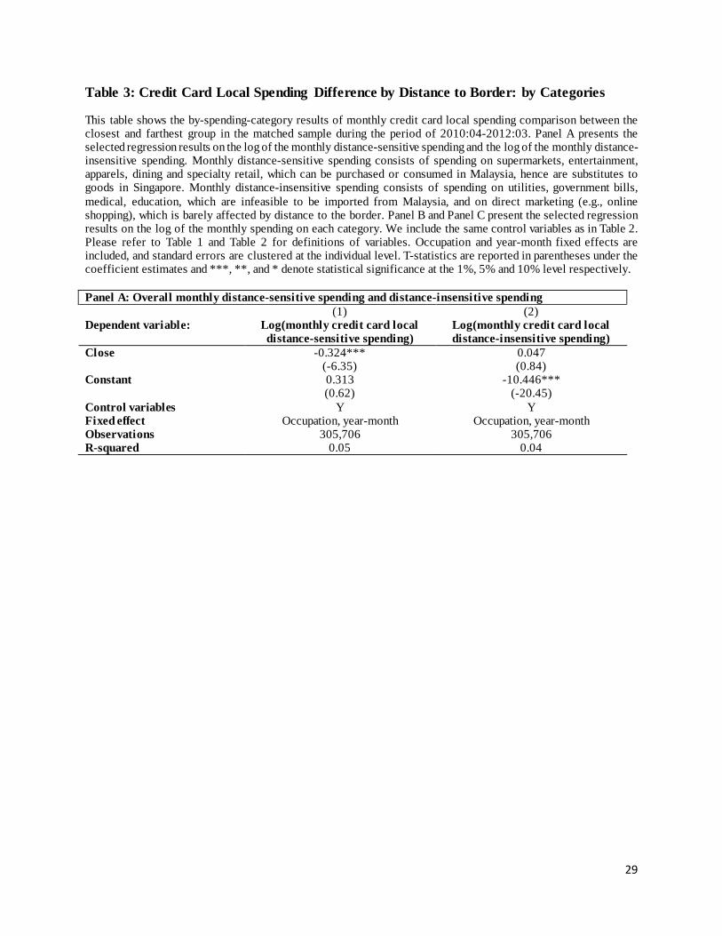
function of distance, and is classified as “distance-insensitive” spending. Table 3 reports the

results based on the two broad categories as well as a break-down of the ten spending categories.

[Insert Table 3 about here]

Panel A shows that consumers living in the close locations on average spend 32.4% less than

those living in the far locations in those distance-sensitive categories (column 1). The effect is

statistically significant at 1% level and is economically large. On the other hand, there is little

difference in spending in the distance-insensitive categories between close and far consumers

(column 2). Turning into the specific spending categories, close consumers spend significantly

less in supermarkets, entertainment, apparel and dining (Panel B). Within the distance-insensitive

categories, consistent with the hypothesis, there are no differences in spending on utilities,

government-related expenses, medical service and direct marketing. Close consumers spend

more on education services than far consumers but the effect is economically negligible

(compared to the difference in spending in the distance-sensitive categories).

4.3 The difference in total debit spending within Singapore

In Table 3, we find a significant difference in credit card spending between the close and the far

consumers, especially in those distance-sensitive categories. One potential concern is that

consumers living close to the border may spend more on other instruments such as debit cards or

cash. For example, they may have less access to credit cards, or stores in those locations prefer to

accept debit cards or cash. To address this question, we study the debit spending difference

between the close and far consumers. We augment the sample matching by adding bank balance

as an additional matching variable, since the amount of debit card as well as cash spending is

14

directly determined by the amount in the bank’s checking balance. Similar as in Table 1, close

and far consumers in the modified matched sample are comparable in the observables, as

reflected by insignificant differences in every demographic characteristics.

[Insert Table 4 About Here]

We first examine debit card spending in Panel A of Table 4. A specific institutional feature is

that the debit card issued by the bank can only be used to make purchases within Singapore.

Therefore, 100% of the spending on the debit card occurs locally. First, there is no difference in

debit card spending between consumers living close to the border and those living far from the

border (column (1)). We further classify the debit card spending into distance-sensitive or

distance-sensitive spending categories in a similar fashion.8 Columns (2) and (3) in Table 4 show

that there is no difference between the close and far consumers in the distance-sensitive or

distance-insensitive categories.

Next we study other forms of debit spending, such as ATM and online banking transactions. We

do not have transaction-level information with respect to these debit transactions, for example

the nature and the amount of ATM or online transactions. Instead, we will examine the number

of these debit transactions to proxy for the debit spending with these instruments. Since the bank

account balance, as well as income and other demographics, are well matched in our test sample,

the number of transactions are likely informative about the actual spending using these debit

instruments. Column (1) of Panel B, Table 4 shows that close consumers on average have 4.5%

fewer number of ATM transactions than far consumers. The effect is marginally significant at

10%. On the other hand, there is no difference in between close and far consumers in the number

of online transactions (column (2)). These results in Table suggests that close and far consumers

do not differ in their debit spending, which implies that the impact of cross-border shopping on

local spending is concentrated in credit cards. For the rest of the analysis on local spending, we

will focus on the credit card.

4.4 Comparison of consumers living close to the two borders

8 Spending categories are defined slightly differently in the debit card. The distance-sensitive categories cover supermarkets, entertainment, apparels and other retail, dining, and books and news; and distance-insensitive categories include utilities, postal services, government, medical and health care, education, tour agencies, driving centres, and local transportation.

15

There are two borders through which individuals can reach Malaysia (by land) from Singapore.

Both borders are far from the city (Singapore) center (can be seen in Figure A1 in the Appendix

A), but only one is relevant for our analysis on cross-border shopping. The Malaysian city across

the Tuas border is agricultural and has no shopping facilities, which is why we focus on the

distance to the Johor Bahru (JB) border in our main analysis (Table 2 and 3). In addition, we

exploit the exogenous difference between the two borders in their access to shopping amenities

for further identification. Specifically, we compare credit card spending of consumers living

close to the JB border with consumers living close to the Tuas border. If there are other

unobservable factors related to consumer’s proximity to the Malaysian border that determine

spending behavior, a comparison between consumers living close to the two borders that have

different access to shopping amenities would help us identify the cross-border shopping effect.

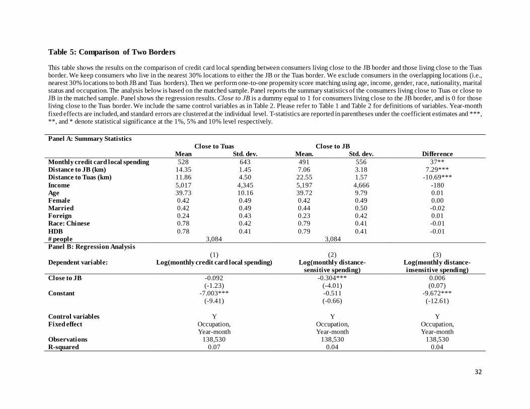
Similar as before, we classify consumers as being “close” to the Tuas border if they live in the

nearest 30% locations to the Tuas border. In this analysis, we include only individuals who are

either close to the JB border or close to the Tuas border (but not close to both). The dummy

variable close to JB is equal to 1 for consumers living close to the JB border (with shopping

amenities), and is equal to 0 otherwise. In order to control for differences in income, wealth and

other demographics between the two samples, we perform a one-to-one propensity score

matching using the same set of explanatory variables as in the main analysis. Panel A of Table 4

reports the summary statistics of the matched sample of consumers living close to the JB border

vs. consumers living close to Tuas. After propensity score matching, the two samples are

observationally similar: the differences in income, age, fraction of consumers who are female,

married, foreign, ethnically Chinese, or living in HDB are statistically insignificant. Even after

matching, consumers living close to the JB border spend significantly less in Singapore than

those living close to the Tuas border.

[Insert Table 5 About Here]

Panel B of Table 4 shows the regression result of the spending difference between the two

groups of consumers. Column 1 shows that on average the total credit card local spending for

consumers live close to the JB border is 9.2% less than the total credit card spending for

consumers living close to the other border (Tuas) with no shopping amenities. Furthermore,

consumers close to the JB border spend 30.4% less (statistically significant at 1%) in distance-

16

sensitive categories (column 2), and have no difference in spending on the distance-insensitive

categories (column 3). Taken together, results in Table 4 suggest that consumers close to the JB

border spend less in Singapore more consistent with the cross-border shopping channel.

4.5 Relocation Subsample

In the main analysis (Table 2 and 3), we exclude consumers who have changed their residential

address in our sample period. In this section, we focus on the relocations subsample and study

whether, after the move, consumers change their spending pattern in Singapore that is related to

the change in the distance to the JB border.

For this analysis, we keep individuals who have had a move in the full sample during our period,

and who lived in the extreme locations before the move (i.e., either close or far locations). We

have a total of 7,325 individuals in the relocation subsample, out of which 785 individuals have

moved either from close to far locations, or from far to close locations. We estimate the

following specification,

𝑦𝑖 ,𝑡 = 𝛼 + 𝛽11𝑏𝑒𝑓𝑜𝑟𝑒 𝑚𝑜𝑣𝑒 𝑐𝑙𝑜𝑠𝑒 + 𝛽21𝑎𝑓𝑡𝑒𝑟 𝑚𝑜𝑣𝑒 + 𝛽31𝑐𝑙𝑜𝑠𝑒 𝑡𝑜 𝑓𝑎𝑟 + 𝛽41𝑓𝑎𝑟 𝑡𝑜 𝑐𝑙𝑜𝑠𝑒 + 𝛽5𝑋𝑖,𝑡 + 𝛾𝑡 + 𝜖𝑖,𝑡 ,

where 1𝑏𝑒𝑓𝑜𝑟𝑒 𝑚𝑜𝑣𝑒 𝑐𝑙𝑜𝑠𝑒 is equal to 1 if consumers live close to the JB border before the move

and 0 otherwise, 1𝑎𝑓𝑡𝑒𝑟 𝑚𝑜𝑣𝑒 is equal to 1 in months after the move and 0 otherwise, 1𝑐𝑙𝑜𝑠𝑒 𝑡𝑜 𝑓𝑎𝑟

is equal to 1 in months after the move and if consumers move from close to far from the border,

1𝑓𝑎𝑟 𝑡𝑜 𝑐𝑙𝑜𝑠𝑒 is equal to 1 in months after the move and if consumers move from far to close

locations. The definitions of close and far are the same as in the main analysis, and we include

the same set of control variables and year-month fixed effects in the regression. The coefficient

on 1𝑐𝑙𝑜𝑠𝑒 𝑡𝑜 𝑓𝑎𝑟 captures the change in spending for consumers who move from close to far,

relative to the consumers who used to live in close locations and did not move too distant from

the JB border. Similarly, the coefficient on 1𝑓𝑎𝑟 𝑡𝑜 𝑐𝑙𝑜𝑠𝑒 captures the change in spending for

consumers who move from far to close, relative to those who used to live in far locations and did

not move too close to the JB border. Our hypothesis is that for consumers who moved

(significantly) away from the border, cross border shopping becomes less appealing and

therefore we expect them to increase spending in Singapore after the move, and hence a positive

coefficient on 1𝑐𝑙𝑜𝑠𝑒 𝑡𝑜 𝑓𝑎𝑟 . Along the same line of thought, we expect those who moved from far

17

to close locations to reduce their spending in Singapore after the move and the coefficient

estimate on 1𝑓𝑎𝑟 𝑡𝑜 𝑐𝑙𝑜𝑠𝑒 should be negative.

Table 5 reports the regression results on the relocation subsample. Column 1 shows the

regression on the total credit card spending and results are statistically insignificant. In addition,

there are no spending differences before and after the move in the location-insensitive categories

(column 3). However, column 2 shows strong evidence that consumers who moved from far to

close spend considerably less (by 44%) in the distance-sensitive categories after the move,

relative to those who lived in far locations and did not move much closer to the JB border. The

effect is statistically significant at 1%. For consumers who moved from close to far, they

increase their spending in Singapore by 12.1% in the distance-sensitive categories relative to

those who lived in the close locations and did not move too far from the border, but the effect is

statistically insignificant. Taken together, the results are broadly consistent with the hypothesis

that consumers increase (decrease) their spending in Singapore after they move farther (closer) to

the border.

[Insert Table 6 About Here]

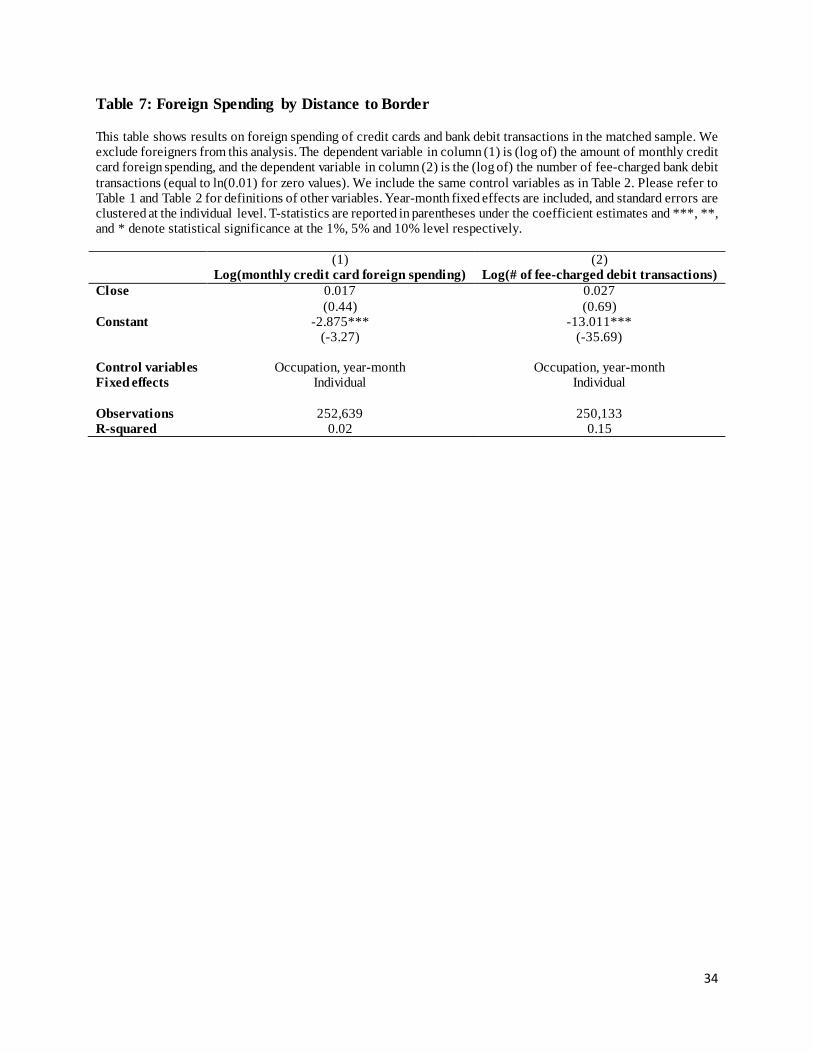
4.7 Foreign Spending

If consumers living close to the border reduce their spending within Singapore because they shop

across the border, then we should expect their spending in JB to be higher. Our credit card

spending data allow us to differentiate foreign spending from local spending; however, we do not

know exactly where the foreign spending occurs. Given the data limitation, we can only look at

the behaviour of total foreign spending on credit cards for consumers in the close and far

locations. We drop foreigners from the matched sample in this analysis. This is because that

foreigners are more likely to spend overseas (e.g., in their home countries), which will bias our

inference given that the two locations have different foreigner presence (even after matching, as

in Table 1). Column (1) of Table 7 shows that the coefficient for close dummy to be positive,

consistent with our hypothesis. However, the effect is statistically insignificant.

[Insert Table 7 About Here]

18

We also investigate whether consumers living close to the border have more debit transactions

overseas than those living far from the border. To do so, we use the number of debit transactions

that have incurred fees as a proxy for foreign debit transactions. For the bank consumers in our

study, cash withdrawal and other forms of debit transactions within Singapore involve no fees.

Most of the fee transactions are foreign transactions such as overseas ATM withdrawal or

overseas transfers. Although there could be other types of fees in debit transactions such as late

fees or account maintenance fees, those are unlikely driving our result given that consumers in

these two locations are finely matched on their income, bank’s checking account balance and

other demographics. Therefore, the number of fee-charged debit transactions is a reasonable

proxy to capture foreign debit spending. For the same reason, we remove foreigners from the

matched sample in this analysis. The positive coefficient in column (2) shows that consumers

living close to the border have more fee-charged transactions than those living far from the

border, but the effect is statistically insignificant.

Taken together, results in Table 7 are broadly consistent with the hypothesis that consumers

living close to the border spend more overseas, possibly across the border in Malaysia. The

effects are statistically weak, however, potentially because we cannot exactly identify the

location (or nature) of the foreign spending.

4.6 Tax vs. price effect

So far, we have not been able to identify the channel – prices or taxes that cause people to shop

abroad. To identify the true channel as to why consumers shop across state borders (prices versus

taxes), next we turn to the Nielsen survey data—a product level dataset that can differentiate

between the price and tax effects. This dataset helps us identify for each product (alcohol,

tobacco, milk, eggs, etc.) the quality, the quantity, and the unit price of the product.

Due to the restricted size of the survey data, we carry out our analysis at the daily level.9 To stay

consistent with the absolute distance cut offs used in the main analysis given the sample size, we

need to choose the 20%/80% cut offs in distance to the JB border to identify close and far

consumers in this dataset. We rank all the products in our dataset by their unit price in the

9 As a robustness check, we perform the analysis with the credit card data at the daily frequency as well and the results remain the same.

19

ascending order. Products in the lowest 30% of price distribution products are labelled as low

price items, while those in the top 30% of price distribution are labelled as high price items.

Then we identify, using the same methodology, high vs. low price items within each product

category.10

Panel A of Table 8 shows the regression result by price level across all categories.11

Interestingly, consumers close to the border spend 6% (0.03 x 2) less daily on high price items

than consumers living far from the border (column 1). However, close consumers spend 3%

more daily on high price items than those far from the border (column 2). The results suggest

that there is a substitution effect between the high price and low price items when consumers do

cross-border shopping. They tend to purchase more on the low price items and less on the high

price items in Singapore. It is important to note that the close and the far consumers in the survey

data are comparable in income as well as demographics (Table A1), and thus the finding is

unlikely due to a result of income differences.

[Insert Table 8 About Here]

In Panel B of Table 8, we take a closer look into selected spending categories reported in the

survey data. There is heterogeneity across different spending categories. The category with the

most significant substitution effect (between high price and low price items) is Cigarettes. For

example, close consumers spend 121% less on high price cigarettes in Singapore than far

consumers, while spending 168% more on low price cigarettes in Singapore than far consumers.

This is expected, as the Singapore government charges hefty import duties on cigarettes, creating

an even bigger price gap from cigarettes sold in Malaysia.

4.7 Robustness checks

In this section, we perform various robustness tests. First, we focus only on consumers living in

public housing (HDB) in our matched sample. Consumers living in the private condominiums

10 The spending documented in the survey data is largely spending on groceries and household necessities, which is reflected in the spending categories reported in Table 7. 11 In the analysis using the survey data, we have 485 consumers living in the far or close locations. In order to maximize power of the test, we do not exclude consumers living in the middle 60% of the distance distribution. To facilitate interpretation, we define close – far as our key explanatory variable, which is a variable equal to 1 if consumers live in close locations, and is equal to -1 for those in far locations. It is straightforward to show that the coefficient on the variable close-far is half the difference in spending between the close and far consumers.

20

are likely to be different from those living in HDB on some other unobservable characteristics

that are relevant for spending behavior. We also perform a robustness test by restricting the

sample to Singaporeans only. After propensity score matching, there is still statistically

significant difference in the fraction of foreign consumers between the close and far consumers.

In addition, foreigners may have different spending preferences (with respect to cross-border

shopping) which potentially confound our result. Therefore, we repeat our analysis in Table 2

and Panel A of Table 3 by removing consumers living in the private condominiums (Table A2,

Panel A) and by removing foreign consumers (Table A2, Panel B). Our results are qualitatively

and quantitatively similar.

Next, we test whether our results are sensitive to the specific distance cutoffs to identify close

and far consumers. We consider two alternative definitions of close and far consumers.

Specifically, we use 20% or 40% cut off points in the distance distribution to identify close

consumers, and 80% or 60% cut off points to identify far consumers. We obtain the same result:

close consumers spend significantly less in Singapore than far consumers in the distance-

sensitive categories (Table A3).

Last, we test the robustness of the results in the full sample (before propensity matching). The

potential concern is that the smaller matched sample is not representative. Results in Table A4

show that the main results in Table 2 and 3 (Panel A) carry through in the full sample, and the

effects are quantitatively similar as well.

5. Conclusion

In this paper we ask the following question: why do consumers cross state borders to shop?

Potentally, consumers cross the state border because of price differentials or tax differentials. For

instance, prices could be lower across the border due to cost of production (cheaper labor and

capital) or taxes could be lower across the border because they do not impose a value-added-tax

encouraging the consumers to cross the border.

We use a unique large dataset of all credit cards transactions for over 180,000 consumers for

over 24 month time period from 2010-2012 from the largest financial institution in Singapore.

We compare the spending patterns of the consumers who live close to the border to the spending

pattern of the consumers who live far away from the border, in substitutable and non-

21

substitutable spending categories. To further identify the channel as to why consumers shop

across state borders (prices versus taxes) we supplement our credit card dataset with the Nielson

survey data that allows us to differentiate the price versus the tax effects. The Nielson data has

detailed product level purchase information for a representative set of 1,214 households in

Singapore over a 36 month time period from 2009-2012.

We find that consumers in Singapore living within 7km of the Johur Bharu border spend 3% less

on their credit cards than the consumers in Singapore living 21km away from the border.

Furthermore, we find that the effect is only prominent for transactions in substitutable categories.

For instance, spending is less in the supermarkets and apparel by 46% and there is no difference

in utilities or government bills. Next, looking at the Nielson survey data, we find that within a

product like cigarettes, consumers living close to the border spend less on cigarettes in Singapore

and more specifically, they spend less on more expensive cigarettes. This suggests that there is

both a tax and a price effect that is pushing the consumers to shop across the border. It is

important to note that our estimate from the diff-in-diff identification strategy should be

interpreted as a lower bound of the cross border shopping effect. In other words, we can only

show the difference in spending between the consumers living close to the border to Malaysia

and those living far from the border. It is plausible that the 7% VAT as well as higher prices in

Singapore encourages all Singaporeans to cross the border and shop in Malaysia.

Our results have policy implications. The VAT of 7% encourages Singaporeans to cross the

border to shop in Malaysia, causing a drop in tax revenue for Singapore and hurting sales of

small businesses close to the Malaysian border. An alternative could be for the Singapore

government is to pursue a tax policy that charges a slightly higher marginal income tax rate and

lowers the VAT keeping the total tax revenue the same but discourating the consumers to cross

state border to shop for goods and services. This will help the merchants in reducing cross border

shopping but could potentially encourage employees to shift taxable income abroad. However, it

is unlikely that consumers will shift taxable income abroad since Singapore would still have a

very low tax rate compared to majority of the countries in the world.

22

References

Aaronson, Daniel, Sumit Agarwal, and Erik French, 2012, “Spending and Debt Response to Minimum Wage Hikes,” American Economic Review, 102(7), 3111-39.

Agarwal, Sumit, Amit Bubna, and Molly Lipscomb, 2013, “Timing to the Statement: Understanding Fluctuations in Consumer Credit Use,” University of Virginia Working Paper.

Agarwal, Sumit, Chunlin Liu, and Nicholas Souleles, 2007, "The Reaction of Consumption and Debt to Tax Rebates: Evidence from the Consumer Credit Data," Journal of Political Economy, 115(6), 986-1019.

Agarwal, Sumit and Leslie McGranahan, 2013, “Consumption Response to State Sales Tax Holidays,” Federal Reserve Bank of Chicago Working Paper.

Agarwal, Sumit and Wenlan Qian, 2013, “Consumption and Debt Response to Fiscal Stimuli: Evidence from a Large Panel of Consumers in Singapore,” NUS Working Paper.

Austan Goolsbee. 1999. In a World Without Borders: the Impact of Taxes on Internet Commerce, Quarterly Journal of Economics,

Bertrand, Marianne, and Adair Morse, 2009, “What Do High-Interest Borrowers Do with their Tax Rebate?", American Economic Review, 99(2), 418-423 Brian G. Knight and Nathan Schiff. 2010. Spatial Competition and Cross-Border Shopping: Evidence from State Lotteries. Working paper

Gross, Tal, Matthew Notowidigdo, and Jialan Wang, 2012, “Liquidity Constraints and Consumer Bankruptcy: Evidence from Tax Rebates,” The Review of Economics and Statistics, forthcoming

Jappelli, T., Pischke, S., and Souleles, N.S., 1998, “Testing for Liquidity Constraints in Euler Equations with Complementary Data Sources,” The Review of Economics and Statistics, 80, pp. 251-262.

Johnson, David, Jonathan Parker, and Nicholas Souleles, N.S., 2006, "Consumption and Tax Cuts: Evidence from the Randomized Income Tax Rebates of 2001," American Economic Review, 96, 1589-1610.

Joseph J. Doyle, Jr. 2006. $2.00 Gas! Studying the Effects of a Gas Tax Moratorium. Working paper

Lesley Chiou and Erich Muehlegger. 2008. Crossing the Line: The Effect of Cross Border Cigarette Sales on State Excise Tax Revenues. Working Paper

Lucas W.Davis. The Effect of Preferential VAT Rates Near International Borders: Evidence From Mexico. Working paper

23

Marcus Asplund, Richard Friberg and Fredrik Wilander. Demand and Distance: Evidence on Cross-Border Shopping. 2005. Working paper

Roger H. Gordon and Soren Bo Nielsen. 1999. Tax Avoidance and Value-added VS. Income Taxiation in an Open Economy. Working paper.

Shapiro, M.D., and Slemrod, J., 2003a, “Consumer Response to Tax Rebates,” American Economic Review, 93, pp. 381-396.

Shapiro, M.D., and Slemrod, J., 2003b, “Did the 2001 Tax Rebate Stimulate Spending? Evidence from Taxpayer Surveys,” in Tax Policy and the Economy, ed. Poterba, J., Cambridge: MIT Press.

Souleles, N.S., 1999, “The Response of Household Consumption to Income Tax Refunds,” American Economic Review, 89, pp. 947-958.

Souleles, N.S., 2000, “College Tuition and Household Savings and Consumption,” Journal of Public Economics, 77(2), pp. 185-207.

Souleles, N.S., 2002, “Consumer Response to the Reagan Tax Cuts,” Journal of Public Economics, 85, pp. 99-120.

Stephens, M., 2003, “3rd of tha Month: Do Social Security Recipients Smooth Consumption Between Checks?” American Economic Review, 93, pp. 406-422.

Stephens, M., 2005, “The Consumption Response to Predictable Changes in Discretionary Income: Evidence from the Repayment of Vehicle Loans,” Carnegie-Mellon University, Working Paper.

Stephens, M., 2006, “Paycheck Receipt and the Timing of Consumption,” The Economic Journal, 116 (513), pp. 680-701.

24

Figure 1: Kernel Densities of the Matched Sample Characteristics

This figure shows the kernel density of the distributions of age, income and the bank checking account balance of the matched sample. closest refers to the locations within the nearest 30% distance to the Malaysia (JB) border, where farthest refers to locations in the top 30% of distance to the Malaysia (JB) border.

0.0

1.0

2.0

3.0

4D

en

sit

y

2 0 40 60 80age

close fa r0

.00

00

5.0

00

1.0

00

15

.00

02

De

ns

ity

0 10000 20000 30000 40000 50000income

close fa r

0.0

00

02

.00

00

4.0

00

06

De

ns

ity

0 50000 100000 150000 200000check ing accoun t ba lance

close fa r

25

Figure 2: Unconditional Mean of Monthly Credit Card Local Spending

This figure shows the mean credit card local spending during our sample period for the close (treatment) and far (control) group in the matched sample. Close refers to the locations within the nearest 30% distance to the Malaysia Johor Bahru (JB) border, where far refers to locations in the top 30% of distance to the Malaysia Johor Bahru (JB) border. Panel A shows the average of the total credit card spending, credit card spending on the distance-sensitive, and distance-insensitive categories respectively. Please refer to Table 3 for definitions of distance-sensitive and distance-insensitive spending categories. Panel B shows the average credit card spending of selected spending categories: supermarket and dining (distance-sensitive) in the top 2 panels, utilities and direct market (distance-insensitive) in the bottom 2 panels. The reported spending amount is in local currency (Singapore dollars). The average exchange rate during our sample period is 1SGD = 0.78 USD (source: Monetary Authority of Singapore). Panel A

$350

$400

$450

$500

$550

$600

$650

$700

Monthly total credit card local spending

Close Far

$50

$70

$90

$110

$130

$150

$170

$190

$210

$230

$250

Monthly credit card local distance-sensitive spending

Close Far

$50

$55

$60

$65

$70

$75

$80

$85

$90

Monthly credit card local distance-insensitive spending

Close Far

26

Panel B

$5

$10

$15

$20

$25

$30

$35

201004 201007 201010 201101 201104 201107 201110 201201

Supermarkets

Close Far

$30

$35

$40

$45

$50

$55

$60

$65

$70

$75

$80

201004 201007 201010 201101 201104 201107 201110 201201

Dining

Close Far

$5

$10

$15

$20

$25

$30

$35

201004 201007 201010 201101 201104 201107 201110 201201

Utilities

Close Far

$5

$6

$7

$8

$9

$10

$11

$12

$13

$14

$15

201004 201007 201010 201101 201104 201107 201110 201201

Direct marketing

Close Far

27

Table 1: Summary Statistics This table reports summary statistics of our closest and farthest samples in the period of 2010:04-2012:03. Close refers to the locations within the nearest 30% distance to the Malaysia Johor Bahru (JB) border, where far refers to locations in the top 30% of distance to the Malaysia Johor Bahru (JB) border. We exclude individuals who report their address as P.O. Box, foreign address or unknown. We also exclude individuals who relocate during the sample period, which we use for a falsification test reported in Table 4. Further, we exclude individuals/accounts that have inactive credit card spending, i.e., accounts with zero monthly spending for more than or equal to 12 months if the account has the first transaction in 2010:04, the first month in our dataset, or accounts with zero monthly spending for more than or equal to 6 months if the account has the first transaction in other months. Panel A shows the statistics for close and far consumers in the full sample, while Panel B reports the statistics after propensity score matching (based on age, income, race, gender, nationality, property type and occupation). Monthly total credit spending is the amount of the total credit card spending by a typical individual in a typical month. Distance is the direct distance between the individual’s address to the Johor Bahru (JB) border of Singapore and Malaysia measured linearly. Income is the monthly salary in the local currency (SGD). Age is the age reported by the individuals. Female is a dummy variable that takes value of 1 if the individual is a female. Married is a dummy variable that takes value of 1 if the individual is married. Foreign is a dummy variable that takes value of 1 if the individual is a foreigner (non-Singapore citizen). Race: Chinese is a dummy variable that takes value of 1 if the individual’s ethnic group belongs to Chinese. HDB is a dummy variable that takes value of 1 if the individual lives in HDB (public housing in Singapore managed by Singapore Housing and Development Board). All the dollar amounts are in the local currency (SGD), and the average exchange rate during our sample period is 1SGD = 0.78 USD (source: Monetary Authority of Singapore).

Panel A: Full Sample Close Far Variable Mean Std. dev. Mean. Std. dev. Close-far Monthly credit card local spending 464 535 542 663 -78*** Monthly debit card spending 378 361 382 382 -5 Monthly # ATM transactions 0.39 2.11 0.58 2.70 -0.19*** Distance (kilometers) 7.55 3.14 21.03 1.77 -13.48*** Income 4,655 3,671 5,419 4,787 -764*** Bank account balance 18,089 30,989 21,383 34,056 -3,295*** Age 39.46 9.91 40.30 10.36 -0.84*** Female 0.41 0.59 0.44 0.50 -0.03*** Married 0.44 0.50 0.44 0.50 0.01 Foreign 0.20 0.40 0.21 0.40 -0.01* Race: Chinese 0.78 0.42 0.75 0.44 0.03*** HDB 0.83 0.37 0.72 0.45 0.12*** # people 24,185 24,185 Panel B: Matched Sample Close Far Variable Mean Std. dev. Mean. Std. dev. Close-far Monthly credit card local spending 503 603 522 638 -19* Monthly debit card spending 390 378 382 386 8 Monthly # ATM transactions 0.50 2.45 0.57 2.90 -0.08* Distance (kilometers) 7.75 3.14 21.00 1.79 -13.26*** Income 5,208 4,456 5,278 4,548 70 Bank account balance 20,520 34,133 20,930 33,756 -415 Age 40.32 10.16 40.27 10.37 0.05 Female 0.43 0.50 0.44 0.50 -0.01* Married 0.44 0.50 0.44 0.50 0.00 Foreign 0.18 0.39 0.20 0.40 -0.01** Race: Chinese 0.75 0.43 0.75 0.43 0.00 HDB 0.74 0.44 0.74 0.44 -0.01 # people 6,786 6,786

28

Table 2: Credit Card Local Spending Difference by Distance to Border This table shows the results of monthly total credit card local spending comparison between the close and far group in the matched sample during the period of 2010:04-2012:03. We keep individuals whose residential addresses are either in the close and far locations, which are defined in Table 1. Close is a dummy that takes a value of 1 if the individual is in the closest 30% location or 0 otherwise. Please refer to Table 1 for definitions of other variables. Occupation and year-month fixed effects are included, and standard errors are clustered at the individual level. T-statistics are reported in parentheses under the coefficient estimates and ***, **, and * denote statistical significance at the 1%, 5% and 10% level respectively. (1) Log(monthly credit card local spending) Close -0.021 (-0.42) Log(income) 0.604*** (15.06) Log(age) 1.189*** (9.88) Female -0.257*** (-4.80) Married 0.205*** (3.71) HDB -0.366*** (-5.98) Foreign 0.049 (0.65) Race: Chinese 0.439*** (4.46) Race: Malay -0.682*** (-5.09) Race: Indian -0.466*** (-3.68) Professional -5.692*** (-11.34) Constant -0.021 (-0.42) Fixed effect Occupation,Year-month Observations 305,706 R-squared 0.08

29

Table 3: Credit Card Local Spending Difference by Distance to Border: by Categories

This table shows the by-spending-category results of monthly credit card local spending comparison between the closest and farthest group in the matched sample during the period of 2010:04-2012:03. Panel A presents the selected regression results on the log of the monthly distance-sensitive spending and the log of the monthly distance-insensitive spending. Monthly distance-sensitive spending consists of spending on supermarkets, entertainment, apparels, dining and specialty retail, which can be purchased or consumed in Malaysia, hence are substitutes to goods in Singapore. Monthly distance-insensitive spending consists of spending on utilities, government bills, medical, education, which are infeasible to be imported from Malaysia, and on direct marketing (e.g., online shopping), which is barely affected by distance to the border. Panel B and Panel C present the selected regression results on the log of the monthly spending on each category. We include the same control variables as in Table 2. Please refer to Table 1 and Table 2 for definitions of variables. Occupation and year-month fixed effects are included, and standard errors are clustered at the individual level. T-statistics are reported in parentheses under the coefficient estimates and ***, **, and * denote statistical significance at the 1%, 5% and 10% level respectively. Panel A: Overall monthly distance-sensitive spending and distance-insensitive spending (1) (2) Dependent variable: Log(monthly credit card local

distance-sensitive spending) Log(monthly credit card local distance-insensitive spending)

Close -0.324*** 0.047 (-6.35) (0.84) Constant 0.313 -10.446*** (0.62) (-20.45) Control variables Y Y Fixed effect Occupation, year-month Occupation, year-month Observations 305,706 305,706 R-squared 0.05 0.04

30

Panel B: Monthly distance-sensitive spending Dependent variable: Log(monthly credit card local spending) (1) (2) (3) (4) (5) Supermarkets Entertainment Apparels Dining Specialty retail Close -0.155*** -0.182*** -0.102*** -0.241*** -0.038*** (-4.45) (-6.35) (-2.61) (-5.69) (-3.43) Constant -3.754*** -0.728*** -3.442*** -0.228 -4.381*** (-11.86) (-2.72) (-9.36) (-0.54) (-43.79) Control variables Y Y Y Y Y Fixed effect Occupation,

Year-month Occupation, Year-month

Occupation, Year-month

Occupation, Year-month

Occupation, Year-month

Observations 305,706 305,706 305,706 305,706 305,706 R-squared 0.03 0.02 0.04 0.04 0.01 Panel C: Monthly distance-insensitive spending Dependent variable: Log(monthly credit card local spending) (1) (2) (3) (4) (5) Utilities Government Medical Education Direct marketing Close 0.038 -0.033 0.032 0.036** 0.025 (0.79) (-1.40) (1.24) (2.32) (0.79) Constant -8.120*** -4.851*** -6.193*** -4.949*** -6.904*** (-18.95) (-22.15) (-26.00) (-35.33) (-22.99) Control variables Y Y Y Y Y Fixed effect Occupation,

Year-month Occupation, Year-month

Occupation, Year-month

Occupation, Year-month

Occupation, Year-month

Observations 305,706 305,706 305,706 305,706 305,706 R-squared 0.03 0.01 0.01 0.00 0.02

31

Table 4: Debit Spending Difference by Distance to Border

This table shows the comparison of debit spending between the close and far group in the matched sample during the period of 2010:04-2012:03. In addition to the other variables used in the original matching, we add the average bank checking account balance in the propensity score matching. Panel A shows the result on debit card spending comparison, and Panel B shows the result on comparison of other debit transactions. In Panel A, the dependent variable in column (1) is the log of the total monthly spending on debit cards; the dependent variable in column (2) is the log of the total monthly spending on debit cards in the distance-sensitive categories (supermarkets, entertainment, apparels and other retail, dining, and books and news); and the dependent variable in column (3) is the log of the total monthly spending on debit cards in the distance-insensitive categories (utilities, postal services, government, medical and health care, education, tour agencies, driving centres, and local transportation). In Panel B, the dependent variable in column (1) is the log of the number of ATM transactions per month (equal to ln(0.01) for zero values); the dependent variable in column (2) is the log of the number of online banking transactions in a month (equal to ln(0.01) for zero values); the dependent variable in column (3) is the log of the number of debit transactions with fee charge (equal to ln(0.01) for zero values). We include the same control variables as in Table 2. Please refer to Table 1 and Table 2 for definitions of variables. Occupation and year-month fixed effects are included, and standard errors are clustered at the individual level. T-statistics are reported in parentheses under the coefficient estimates and ***, **, and * denote statistical significance at the 1%, 5% and 10% level respectively. Panel A (1) (2) (3) Dependent variable: Log(monthly debit card

spending) Log(monthly debit card

distance-sensitive spending)

Log(monthly debit card distance-insensitive

spending) Close 0.024 -0.041 0.077 (0.70) (-0.76) (1.60) Constant 5.283*** 2.635*** 3.707*** (16.16) (5.08) (7.78) Control variables Y Y Y Fixed effects Occupation, year-month Occupation, year-month Occupation, year-month Std. err. cluster Individual Individual Individual Observations 306489 306489 306489 R-squared 0.02 0.05 0.04 Panel B (1) (2) Dependent variable: Log(# ATM transaction) Log(# online transaction) Close -0.045* -0.006 (-1.81) (-0.27) Constant -8.632*** -1.973*** (-34.65) (-9.23) Control variables Y Y Fixed effects Occupation, year-month Occupation, year-month Std. err. cluster Individual Individual Observations 306489 306489 R-squared 0.08 0.03

32

Table 5: Comparison of Two Borders

This table shows the results on the comparison of credit card local spending between consumers living close to the JB border and those living close to the Tuas border. We keep consumers who live in the nearest 30% locations to either the JB or the Tuas border. We exclude consumers in the overlapping locations (i.e., nearest 30% locations to both JB and Tuas borders). Then we perform one-to-one propensity score matching using age, income, gender, race, nationality, marital status and occupation. The analysis below is based on the matched sample. Panel reports the summary statistics of the consumers living close to Tuas or close to JB in the matched sample. Panel shows the regression results. Close to JB is a dummy equal to 1 for consumers living close to the JB border, and is 0 for those living close to the Tuas border. We include the same control variables as in Table 2. Please refer to Table 1 and Table 2 for definitions of variables. Year-month fixed effects are included, and standard errors are clustered at the individual level. T-statistics are reported in parentheses under the coefficient estimates and ***, **, and * denote statistical significance at the 1%, 5% and 10% level respectively. Panel A: Summary Statistics Close to Tuas Close to JB Mean Std. dev. Mean. Std. dev. Difference Monthly credit card local spending 528 643 491 556 37** Distance to JB (km) 14.35 1.45 7.06 3.18 7.29*** Distance to Tuas (km) 11.86 4.50 22.55 1.57 -10.69*** Income 5,017 4,345 5,197 4,666 -180 Age 39.73 10.16 39.72 9.79 0.01 Female 0.42 0.49 0.42 0.49 0.00 Married 0.42 0.49 0.44 0.50 -0.02 Foreign 0.24 0.43 0.23 0.42 0.01 Race: Chinese 0.78 0.42 0.79 0.41 -0.01 HDB 0.78 0.41 0.79 0.41 -0.01 # people 3,084 3,084 Panel B: Regression Analysis (1) (2) (3) Dependent variable: Log(monthly credit card local spending) Log(monthly distance-

sensitive spending) Log(monthly distance- insensitive spending)

Close to JB -0.092 -0.304*** 0.006 (-1.23) (-4.01) (0.07) Constant -7.003*** -0.511 -9.672*** (-9.41) (-0.66) (-12.61) Control variables Y Y Y Fixed effect Occupation,

Year-month Occupation, Year-month

Occupation, Year-month

Observations 138,530 138,530 138,530 R-squared 0.07 0.04 0.04

33

Table 6: Relocation Subsample This table shows results of monthly credit card local spending in response to individual’s change in distance to the border of Singapore and Malaysia due to relocation in the period of 2010:04-2012:03. In this analysis, we retain the individuals who have had a relocation in the full sample during our period, and who lived in the extreme locations (i.e., either close or far) before the relocation. Before move close is a dummy that takes a value of 1 if the consumers live in the closest locations before the relocation. After move is a dummy equal to 1 in months after the move. Close-to-far is dummy variable that takes on a value of 1 for months after the move and if individuals move from the closest to the farthest locations. Far-to-close is dummy variable that takes on a value of 1 for months after the move and if individuals move from the farthest to the closest locations. In the analysis, we include same control variables as in Table 2. Please refer to Table 1 and Table 2 for definitions of other variables. Year-month fixed effects are included, and standard errors are clustered at the individual level. T-statistics are reported in parentheses under the coefficient estimates and ***, **, and * denote statistical significance at the 1%, 5% and 10% level respectively. (1) (2) (3) Log(monthly credit card

local spending) Log(monthly distance-

sensitive spending) Log(monthly distance-insensitive spending)

Before move close -0.095 -0.432*** -0.102 (-1.30) (-5.94) (-1.44) After move 0.506*** 0.342*** -0.011 (6.59) (4.62) (-0.16) Close to far 0.061 0.121 0.014 (0.41) (0.83) (0.10) Fart to close -0.168 -0.440*** -0.060 (-1.09) (-2.93) (-0.42) Constant -8.272*** -4.705*** -9.742*** (-11.33) (-9.52) (-14.43) Control variables Y Y Y Fixed effect Occupation,

Year-month Occupation, Year-month

Occupation, Year-month

Observations 162,801 162,801 162,801 R-squared 0.10 0.05 0.04

34

Table 7: Foreign Spending by Distance to Border This table shows results on foreign spending of credit cards and bank debit transactions in the matched sample. We exclude foreigners from this analysis. The dependent variable in column (1) is (log of) the amount of monthly credit card foreign spending, and the dependent variable in column (2) is the (log of) the number of fee-charged bank debit transactions (equal to ln(0.01) for zero values). We include the same control variables as in Table 2. Please refer to Table 1 and Table 2 for definitions of other variables. Year-month fixed effects are included, and standard errors are clustered at the individual level. T-statistics are reported in parentheses under the coefficient estimates and ***, **, and * denote statistical significance at the 1%, 5% and 10% level respectively. (1) (2) Log(monthly credit card foreign spending) Log(# of fee-charged debit transactions) Close 0.017 0.027 (0.44) (0.69) Constant -2.875*** -13.011*** (-3.27) (-35.69) Control variables Occupation, year-month Occupation, year-month Fixed effects Individual Individual Observations 252,639 250,133 R-squared 0.02 0.15

35

Table 8: Cross-border Shopping: Tax Effect vs. Price Effect This table studies the heterogeneity in spending patterns in item prices by using a detailed survey data from 2008:01-2010:12. It reports results of daily spending on high (low) price items in relation to consumer’s distance to the JB border of Singapore and Malaysia in the period of 2008:01-2010:12. We rank all the products in our dataset by their unit price in the ascending order. Products in the lowest 30% of price distribution products are labelled as low price items, while those in the top 30% of price distribution are labelled as high price items. Panel A reports the regression results of comparison of consumer’s daily spending on high (low) price items between the close and far consumers, and Panel B reports the regression results of comparison of consumer’s daily spending between the close and far consumers by price and by spending category. Close – far is a variable equal to 1 if consumers live in locations in the nearest 20% distance to JB border, and is equal to -1 if consumers live in locations in the nearest 20% distance to JB border. Other control variables include the household income, household size, and race. Day-of-week fixed effect is included, and standard errors are clustered at the household-month level. T-statistics are reported in parentheses under the coefficient estimates and ***, **, and * denote statistical significance at the 1%, 5% and 10% level respectively. Panel A: By Price Level (1) (2) Dependent variable: Log(daily spending

on high price items) Log(daily spending on low price items)

Close-far -0.030*** 0.015*** (-4.05) (3.67) Constant 2.672*** 1.168*** (100.96) (68.42) Control variables Y Y Fixed effect Day of week Day of week Observations 140,786 142,094 R-squared 0.03 0.03

36

Panel B: By Price Level and Spending Category : Log(daily spending)

Electronics and household Baby Care Drugs and nutrients Cigarettes High Low High Low High Low High Low (1) (2) (3) (4) (5) (6) (7) (8)

Close-far -0.010 0.014* 0.072*** 0.007 -0.018* -0.004 -0.603** 0.843* (-1.54) (1.94) (4.37) (0.56) (-1.93) (-0.53) (-2.53) (1.81) Constant 2.159*** 1.173*** 2.851*** 1.767*** 2.562*** 1.302*** 2.868*** -0.601 (78.19) (38.69) (45.27) (35.27) (67.32) (46.15) (5.81) (-0.61) Beverages Alcohol Meat Vegetables, fruits and others High Low High Low High Low High Low (9) (10) (11) (12) (13) (14) (15) (16) Close-far 0.001 0.028*** -0.067** 0.241*** -0.047*** -0.017*** -0.048*** 0.014*** (0.14) (4.39) (-2.16) (6.71) (-3.82) (-3.25) (-8.15) (3.63) Constant 1.772*** 1.136*** 3.187*** 1.383*** 2.289*** 1.180*** 2.192*** 1.133*** (78.21) (46.01) (25.69) (12.20) (57.57) (51.73) (93.36) (65.91)

37

Appendix A: Distance to the Border

The island of Singapore stretches approximately 49 kilometres from East to West and 25 kilometres from North to South with a total land area of 710 km2. The country is divided into twenty-eight planning or postal districts excluding few off-shore islands. Each postal district can further be classified into eighty-three 6-digit postal sectors as shown in figure 1. The northern and western region of Singapore is connected with the adjacent state of Johor in Malaysia through two expressways originating from postal sector seventy-five (Singapore-Johor causeway) and sixty-three (Tuas second link) respectively. We obtained the postal codes at two immigration checkpoints on the border and assume these as the points of entry into Singapore.

For the two spending datasets used in our study, we have the exact 6-digit postal codes for the credit card spending data but only the 2-digit postal sector for the survey data. As a result, we compute linear distances (in kilometers) from the two points of entry to the exact 6-digit postal codes for each consumer in the credit card spending data. For the survey data, we compute linear distances from the two points of entry to the centroid of each (2-digit) postal sector.14

Figure A1: Singapore map showing the eighty-five distinct postal sectors

14 The data collection was performed using ArcGIS software provided by National university of Singapore. All linear distances between the points of entry to each postal code in Singapore was calculated using ArcGIS’s Arcmap platform. Specifically the distance is calculated as follows:

Longitude to radians (if in decimal form omit the division by one million) = (longitude/1000000)*( π /180) Latitude to radians (if in decimal form omit the division by one million) = (latitude/1000000)*( π /180) Distance between two points, with both points' longitudes and latitudes in radians =

arccos(sin(lat1)*sin(lat2)+cos(lat1)*cos(lat2)*cos(lon2-lon1))*6370*0.62

38

Table A1: Selected Summary Statistics of Nielsen Survey Data The dataset we use in this study is from Nielsen survey. This table reports the summary statistics of our closest and farthest samples in the period of 2008:01-2010:12. The “close sample” consists of households who live in the nearest 20% locations to the JB border of Singapore and Malaysia, and the “far sample” consists of households who live in the farthest 20% locations to the JB border. We exclude individuals with a reported monthly income of greater than 10,000. We also exclude observations that have per unit price lower than $1 and/or have more than 10 repeat units in one transaction. Daily total spending is the amount of the total spending by a typical household on a typical day. Distance is the direct distance between the household’s address to the JB border of Singapore and Malaysia measured linearly. Income is the monthly salary in the local currency (SGD) reported by the households. Household size is the number of family members reported by the households. Race: Chinese is a dummy variable that takes value of 1 if the household’s ethnic group belongs to Chinese. All the dollar amounts are in the local currency (SGD). Close Far Variable Mean Std. dev. Mean. Std. dev. Close-far Daily total spending 46.88 33.97 44.98 35.85 1.90 Distance (kilometers) 5.47 2.86 19.36 2.02 -13.89*** Income 3,923 2,360 4,080 2,354 -157 Household size 4.08 1.25 3.70 1.72 0.38*** Race: Chinese 0.73 0.45 0.72 0.45 0.00 # households 220 220

39

Appendix C Robustness Checks

Table A2. Matched Sample: HDB or Singaporean only

This table repeats the analysis in Table 2 and 3 in a subsample of the matched sample during the period of 2010:04-2012:03. In Panel A, we keep only individuals who live in public housing (i.e., HDB), and whose residential addresses are either in the closest and farthest locations. In Panel B, we keep the closest and farthest individuals who are Singaporeans. We include the same control variables as in Table 2 and 3. Occupation and year-month fixed effects are included, and standard errors are clustered at the individual level. T-statistics are reported in parentheses under the coefficient estimates and ***, **, and * denote statistical significance at the 1%, 5% and 10% level respectively.

Panel A: HDB sample (1) (2) (3) Dependent variable: Log(monthly credit card local

spending) Log(monthly credit card local distance-sensitive spending)

Log(monthly credit card local distance-insensitive spending)

Close 0.009 -0.302*** -0.014 (0.15) (-5.20) (-0.22) Constant -6.706*** -0.241 -9.672*** (-12.03) (-0.43) (-17.16) Control variables Y Y Y Fixed effect Occupation,

Year-month Occupation, Year-month

Occupation, Year-month

Observations 226,346 226,346 226,346 R-squared 0.07 0.04 0.04 Panel B: Singaporean sample Close -0.055 -0.288*** -0.038 (-1.01) (-5.17) (-0.62) Constant -5.588*** 0.299 -9.485*** (-10.13) (0.55) (-16.77) Control variables Y Y Y Fixed effect Occupation,

Year-month Occupation, Year-month

Occupation, Year-month

Observations 252,639 252,639 252,639 R-squared 0.07 0.04 0.04

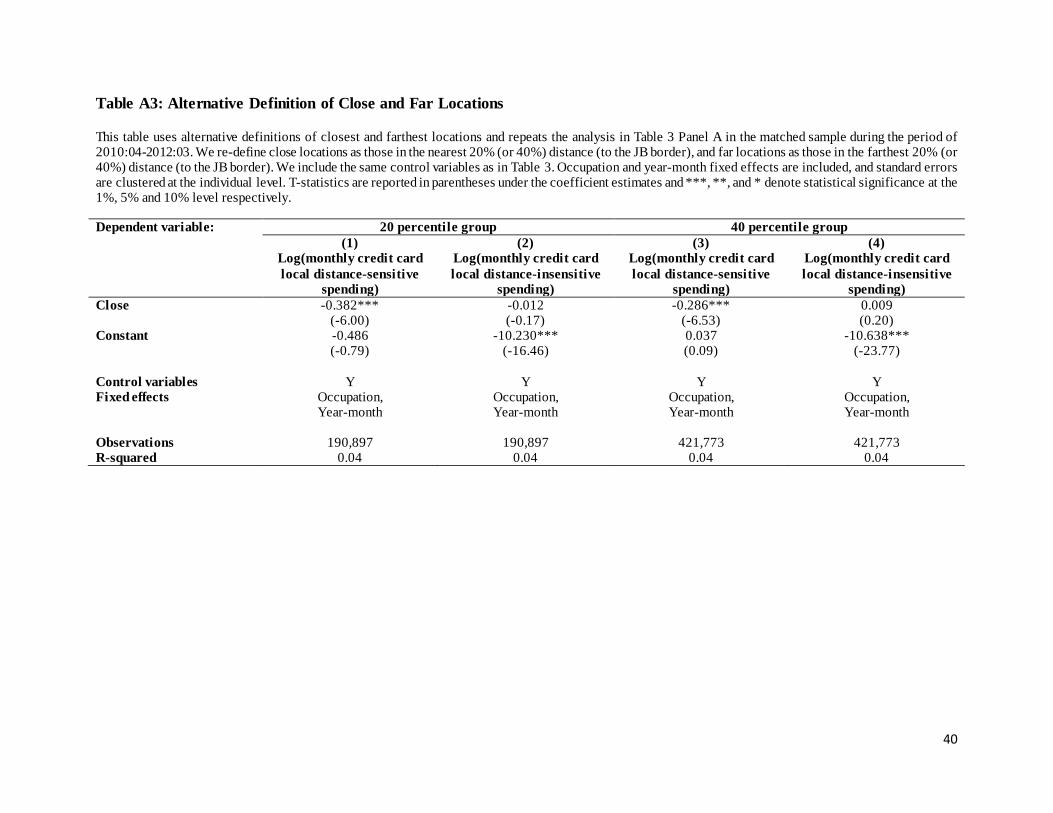
40

Table A3: Alternative Definition of Close and Far Locations

This table uses alternative definitions of closest and farthest locations and repeats the analysis in Table 3 Panel A in the matched sample during the period of 2010:04-2012:03. We re-define close locations as those in the nearest 20% (or 40%) distance (to the JB border), and far locations as those in the farthest 20% (or 40%) distance (to the JB border). We include the same control variables as in Table 3. Occupation and year-month fixed effects are included, and standard errors are clustered at the individual level. T-statistics are reported in parentheses under the coefficient estimates and ***, **, and * denote statistical significance at the 1%, 5% and 10% level respectively.

Dependent variable: 20 percentile group 40 percentile group (1) (2) (3) (4) Log(monthly credit card

local distance-sensitive spending)

Log(monthly credit card local distance-insensitive

spending)

Log(monthly credit card local distance-sensitive

spending)

Log(monthly credit card local distance-insensitive

spending) Close -0.382*** -0.012 -0.286*** 0.009 (-6.00) (-0.17) (-6.53) (0.20) Constant -0.486 -10.230*** 0.037 -10.638*** (-0.79) (-16.46) (0.09) (-23.77) Control variables Y Y Y Y Fixed effects Occupation,

Year-month Occupation, Year-month

Occupation, Year-month

Occupation, Year-month

Observations 190,897 190,897 421,773 421,773 R-squared 0.04 0.04 0.04 0.04

41

Table A4 Full Sample Analysis

This table repeats the analysis in Table 2 and 3 in the full sample (before propensity score matching) during the period of 2010:04-2012:03. We include the same control variables as in Table 2 and 3. Year-month fixed effects are included, and standard errors are clustered at the individual level. T-statistics are reported in parentheses under the coefficient estimates and ***, **, and * denote statistical significance at the 1%, 5% and 10% level respectively.

(1) (2) (3) Dependent variable: Log(monthly credit card local

spending) Log(monthly credit card local distance-sensitive spending)

Log(monthly credit card local distance-insensitive spending)

Close -0.038 -0.385*** -0.004 (-1.41) (-14.06) (-0.13) Constant -6.159*** 0.490* -9.968*** (-23.16) (1.83) (-36.57) Control variables Y Y Y Fixed effect Occupation,

Year-month Occupation, Year-month

Occupation, Year-month

Observations 1,087,946 1,087,946 1,087,946 R-squared 0.07 0.05 0.04