“crowther’s 11th marieb” - uw faculty web...

Supplement to the BBio 242 Laboratory Manual Summer 2017

1

“Crowther’s 11th Marieb” (a guide to your lab manual)

Laboratory exercises in BBio 242 are taken mostly from the Human Anatomy &

Physiology Laboratory Manual by Elaine N. Marieb (“MARE-ibb”), Susan J. Mitchell, and

Lori A. Smith. Please make sure you have the 11th edition of the fetal pig version (2014)!

(You can rent access to this edition, if you prefer, or you can buy a used version. You

can purchase this on its own or as a bundle with PhysioEx 9.1, which you will need as

well.) This lab manual is nice in some respects, but includes more details, activities, and

questions than we can handle. For each assigned exercise, this “Crowther’s 11th Marieb”

guide will tell you what to do and what not to do!

You can print out this entire manual at the start of the quarter, or you can print out

individual labs as you go. Please make double-sided prints if possible. Some pages

have been intentionally left blank so that the pages that you must hand in are separate

from the pages that you may want to keep.

Too much, Dr. Marieb! Too much!


2

Lecture-in-Lab June 19, 2017

Today’s “lab” will consist of lecture and discussion activities not found in the lab manual.

There is no homework due today. Please come to the lab room (room 267 of Discovery

Hall).

Dissection Exercise 3: Identification of Selected Endocrine Organs of the Fetal Pig

June 21, 2017 Goals

• Prepare the pig for observation by opening the ventral body cavity (Activity 1).

• Identify and name the major endocrine organs on a dissected pig (Activity 2).

Safety

Come to lab dressed appropriately: long hair under control, long pants or long skirt,

shoes that fully protect the feet. Once in lab, use eye and hand protection as needed.

Instructions

With your lab partner, get a fetal pig from your instructor. With gloves on, take the pig to

a sink, cut open the bag at one end, and pour any excess fluid down the drain. Put the

pig on a dissecting tray.

Complete Activity 1 (Opening the Ventral Body Cavity) and Activity 2 (Identifying Organs)

as described on the lab manual. As you do so, keep in mind the following general

dissection tips (which apply to dissections in general, not just today’s exercise):

• Use reference pictures from your lab manual, dissection manuals, and/or the

Internet to help you find what you’re looking for.

• Once you enter the body cavity, use the scalpel and scissors sparingly. When

possible, push things around with the blunt probe rather than cutting.

• Use spray bottles to keep the animal’s interior moist.

• Use your personal fume hoods to control odors.

• Take breaks inside and/or outside the lab as needed.

• Take turns with your lab partner, so that both of you get to “drive” with the

dissection tools and “navigate” with the anatomical “maps.”


3

• You are welcome to take pictures for study purposes, but please do not share on

social media. Sketching is optional, but very helpful for some people.

After you have found the organs mentioned in Activity 2, your instructor will ask you to

show them to him/her and will initial your worksheet when you have been successful.

Then bag up your pigs and label the bags!

Finally, look at a 3D human torso model and compare the endocrine organs there to

what you saw in your pig.


4


5

Worksheet for Dissection Exercise 3: Identification of Selected Endocrine Organs of the Fetal Pig

Due June 21, 2017 Names: Organ checklist (for reference; fill in “Hormones secreted” column)

Anatomic region Organ/gland Hormone(s) secreted (of those listed below*)

Neck and thoracic cavity Trachea

Neck and thoracic cavity Thymus

Neck and thoracic cavity Thyroid gland

Neck and thoracic cavity Heart

Neck and thoracic cavity Lungs

Abdominopelvic cavity Stomach

Abdominopelvic cavity Spleen

Abdominopelvic cavity Small intestine

Abdominopelvic cavity Pancreas

Abdominopelvic cavity Large intestine (colon)

Abdominopelvic cavity Kidneys

Abdominopelvic cavity Adrenal glands

Abdominopelvic cavity Gonads (testes or ovaries)

*Hormone list: adrenaline (epinephrine), aldosterone, cortisol, estrogen, glucagon,

immune system hormones, insulin, progesterone, testosterone, triiodothyronine (T3),

thyroxine (T4)

Instructor’s initials, indicating successful identification of the above organs: _______


6

Dissection Review 1. 2. 3. 4. 5.

Metacognition

What part of today’s lab will be most important for you to review before the next test?

Why?


7

PhysioEx Exercise 4: Endocrine System Physiology

June 21, 2017 / Due June 28, 2017

Goals

• To understand the relationships between Thyrotropin Releasing Hormone (TRH),

Thyroid Stimulating Hormone (TSH), and the thyroid hormones triiodothyronine

(T3) and thyroxine (T4) (Activity 1).

• To understand how metabolic rate is measured (Activity 1).

• To determine the effects of pituitary or thyroid gland perturbations on metabolic

rate (Activity 1).

• To estimate patients’ plasma glucose levels based on a standard curve (Activity

2).

• To understand the relationships between insulin, glucose, and diabetes mellitus

(Activity 2).

• To see how sex hormones like estrogen affect bone density, and how bone

density can be measured and reported (Activity 3).

Instructions

Please do Activities 1 through 3 of PhysioEx Exercise 4 ("Endocrine System

Physiology"), found on pages PEx-59 through PEx-74 in your lab manual:

• Activity 1: Metabolism and Thyroid Hormone

• Activity 2: Plasma Glucose, Insulin, and Diabetes Mellitus

• Activity 3: Hormone Replacement Therapy

Log in to MasteringAandP.com, select “Study Area (myA&P),” select “PhysioEx 9.1,”

click on the blue text link (PhysioEx 9.1), and do the online simulations described in the

manual.

Important: You do NOT need to turn in answers to the questions shown in your lab

manual or online. Instead, for each activity, type a brief “lab report” – which you will

submit to Canvas – with the following labeled components:

• EXPERIMENT

o In about 2-4 sentences, describe the experiment that was done. (What was

the basic setup? What variable was manipulated? What responses were

measured?) If the experiment was similar to that in a previous activity, you

can say, "This was similar to Activity X, except that...." Use correct units

(millimeters, millivolts, seconds, etc.).


8

• HYPOTHESIS

o Before you perform the experiment, predict how the key data will come out.

You will not be graded on the correctness of your prediction, but making

predictions will help you learn more.

• RESULTS

o What key data (quantitative and/or quantitative) were generated from this

experiment? Use correct units (millimeters, millivolts, seconds, etc.). You

do not need to include every table or graph generated by the website, but

do show me the most important bits (either summarized in the website's

format, or presented in your own format) and briefly explain them to me in

words. If you are using figures or tables generated automatically by the

website, you may include screen captures, but please crop them for

simplicity/clarity, as needed. Please do not take photographs of your

computer screen with your phone, as the resolution will not be good.

• CONCLUSION

o In about 2-3 sentences, state whether the data fit your prediction, and what

conclusions you can draw. Conclusions relate directly to the data but go

beyond reporting them. Try to explain (briefly) any key connections

between the experiment and material we are covering in lecture. Why are

the data important or interesting?

Below is an example of how these sections might be completed for PhysioEx Exercise 3

(Neurophysiology of Nerve Impulses), Activity 3 (The Action Potential: Threshold).

• Experiment: Stimuli of different voltages are applied to the axon of a neuron (at site S), and

membrane potentials are recorded farther down the axon (at sites R1 and R2). The question is how

the axon responds to different levels of input.

• Hypothesis: I predict that the stimulus threshold will be above 10 mV but below 50 mV, so that

the lowest stimulus voltage does not trigger an action potential, but the highest stimulus voltage

and perhaps some intermediate ones do trigger an action potential.

• Results: The lowest stimulus voltage, 10 mV, did not cause a response at R1 or R2. All of the

other stimuli (20-50 mV) resulted in identical action potentials at R1 and R2. See table below.

Stimulus voltage

(mV)

Peak value at R1

(µV)

Peak value at R2

(µV)

Action potential

10 0 0 No

20 100 100 Yes

30 100 100 Yes


9

40 100 100 Yes

50 100 100 Yes

• Conclusion: Action potentials are “all or none”; they either fire (if depolarization at the axon

hillock is sufficient) or they don’t.

Your lab manual and the PhysioEx program should have all of the information that you

need, but you are also allowed to consult outside sources. If you do use outside

sources, please cite them, using quotation marks for direct quotes.


10

Exercise 27: Functional Anatomy of the Endocrine Glands [& More!] June 26, 2017

Goals

• To observe adrenal, pancreas, parathyroid, pituitary (hypophysis), and thyroid

cells under the light microscope.

• To measure blood glucose levels before and after feeding, and to consider their

hormonal regulation.

Universal precautions regarding the use of human blood in laboratories

In today’s lab, you will collect tiny amounts of your own blood. Medical history and

examination cannot reliably identify whether someone is infected with HIV or other blood-

borne pathogens. Therefore, all students and instructors must use precautions when

handling blood. This approach, referred to as “Universal Precautions,” has been

recommended by the Centers for Disease Control and Prevention (CDC) and advises

you to consider all blood as infectious.

This laboratory experience has been reviewed and approved by UW’s Office of

Environmental Health and Safety (EH&S).

Part A: histology

The main activity of this lab will be measuring the glucose levels of your own blood

before and after eating. When you are not doing this, you should look at five slides of

endocrine tissues:

• Adrenal gland

• Pancreas

• Parathyroid gland

• Pituitary gland (hypophysis)

• Thyroid gland

Microscope slides are sometimes labeled with cryptic abbreviations. Here are some common ones to be aware of:

• h&e = hematoxylin & eosin stain (turns the nucleus blue and the cytoplasm pink, orange, or red)

• l.s. = longitudinal section

• sec = section

• s.m. = smear

• x.s. = cross-section


11

And here are some tips for drawing what you see on a slide:

• Do not draw everything in an entire field of view unless an “overview” sketch is desired. If trying to record the appearance of individual cells, draw a small number of cells (1-2) in as much detail as possible. Sometimes it is best to do a two-part drawing, with an overview plus an inset.

• Don’t draw details that you can’t actually see (even if they are in shown in other pictures).

• Label structures (e.g., “nucleus”) that you can see.

• Indicate the total magnification (ocular lens X objective lens) of the view on which your drawing is based.

Part B: blood glucose levels

If possible, please have breakfast before 9am and do not ingest any more calories until

lab.

One at a time, you will sit on a chair next to our designated blood collection bench with a

sharps container within arm’s reach. You will prick your finger with a lance and massage

the pricked finger to release an adequate volume of blood.

Once enough blood has accumulated (one large drop should be enough), let your

instructor know and he/she will attach the testing strip to the glucose meter. You will

then put your finger against the testing strip until enough blood is collected. You will be

given a Band-Aid for the puncture site. The used lancet goes into the red biohazard

sharps container (hard plastic); other blood-stained materials go into the biohazard bag.

Your blood sample will be analyzed with a cheap but efficient blood glucose meter,

available at local drug stores for $10-$70. The glucose meter oxidizes glucose,

generating electrons that are detected by an electrode.

Your instructor will write down your current glucose level, the date and time, and the

approximate time of your last meal/snack, and enter these data in a spreadsheet. You

may see your own glucose reading if you wish, though all data will be anonymized before

they are shared with the class.

You will leave the lab to have a snack and then will return to the lab, resume looking at

slides, and measure your blood glucose again just before the end of lab.

The anonymized blood glucose dataset will be shared on the class website so that you

can download and analyze it later.


12

Appendix: basic statistical tests

In analyzing your blood glucose data, you will test your hypothesis with a basic statistical

test. Three of the most common analyses are the t-test, ANOVA, and linear regression.

T-test

A t-test answers the question, “Are the means of these two groups of values more

different than we would expect to occur by chance?” For example, the class’s blood

glucose values before eating pizza will never be EXACTLY the same as its values after

eating pizza, but the t-test tells the probability of seeing the observed difference (or

something more extreme), if there were truly no difference in glucose values before and

after eating pizza. This probability is the p value. For historical reasons, and by popular

convention, a p value of less than 0.05 is generally considered “statistically significant.”

That is, if an observed difference would occur less than 5% of the time if there were truly

no difference between groups, the difference is considered “real.”

T-tests come in several varieties: they can be paired or unpaired, and can be 1-tailed or

2-tailed.

• In a paired t-test, each specific value in one group is matched or paired with a

specific value in the other group. This is because both values came from the

same person, or have some other common factor. In studying the effect of pizza

on blood glucose levels, one could do a paired t-test in which each subject’s pre-

pizza value would be paired with his/her post-pizza value. The alternative, an

unpaired t-test, would be used if we made one group fast and measured their

fasting blood glucose levels, then fed pizza to a different group and measured that

other group’s fed blood glucose levels.

• In a 1-tailed t-test, the two groups are tested for a difference in a certain direction

(e.g., the fed glucose values will be HIGHER than the fasting glucose values). In

a 2-tailed t-test, no direction is specified (e.g., the fed glucose values will be

DIFFERENT than the fasting glucose values). The “tails” refer to the tails of a bell

curve; in a 1-tailed test, you are focusing on one end (tail) of the curve, i.e., a

difference in one specific direction. It is important to specify the number of tails in

your t-test because the p value depends on the number of tails.

There are multiple ways to do a t-test in Excel. The simplest way is to use the following

formula:

= T.TEST(array1,array2,tails,type)

where tails is the number of tails (1 or 2) and type is 1 (paired), 2 (unpaired, equal

variances in the 2 samples), or 3 (unpaired, unequal variances in the 2 samples). If


13

doing an unpaired t-test, we generally prefer to use the unequal variances version, so as

to make the fewest assumptions necessary.

The number you get out from this formula is simply a p value between 0 and 1.

More information about the Excel T.TEST function can be found online, e.g., at

https://support.office.com/en-us/article/T-TEST-function-d4e08ec3-c545-485f-962e-

276f7cbed055.

An alternative way of doing a t-test in Excel is to use the Analysis TookPak add-in.

Activating this add-in might be different in different versions of Excel, but on a typical PC,

one proceeds as follows: File => Options => Add-Ins => Manage: Excel Add-Ins (click

“Go…”) => Check the Analysis ToolPak => Click “OK.” Once this is done, the DATA tab

of Excel should include a Data Analysis option, from which you can select various types

of t-tests. In this option, you will need to specify a hypothesized mean difference

(generally 0) and an alpha level (generally 0.05, corresponding to the usual significance

cutoff of p < 0.05).

ANOVA

In its simplest form, an ANOVA (short for analysis of variance) is essentially a t-test for

comparing more than two groups. An ANOVA compares the variation within each group

to the variation between the groups. The smaller the former is relative to the latter, the

lower the p value. For example, imagine that Groups A, B, and C have mean scores of

70, 71, and 72, respectively. These groups may or may not be significantly different,

depending on how much variation there is in each group. If each group’s individual

values were all within a tenth of a point of the group’s mean (e.g., Group A includes

values of 69.9, 69.9, 70, 70, 70, 70, 70.1, and 70.1), the groups would be significantly

different according to an ANOVA. If the groups overlapped much more, they would not

be statistically significantly different. ANOVAs can be performed in Excel using the

Analysis TookPak (which can be installed according to the instructions above).

Linear regression

A linear regression determines how much of the variability in a variable (say, Y) can be

explained by another variable (say, X). The closeness of the linear relationship between

X and Y can be quantified with Pearson’s correlation coefficient, r, or with the square of

this value, R2, which is the fraction of the variation in Y that can be explained by X.

Values for r can range from -1 (a perfect negative correlation) to 1 (a perfect positive

https://support.office.com/en-us/article/T-TEST-function-d4e08ec3-c545-485f-962e-276f7cbed055

https://support.office.com/en-us/article/T-TEST-function-d4e08ec3-c545-485f-962e-276f7cbed055


14

correlation); values for R2 can range from 0 (no correlation) to 1 (a perfect correlation).

One can also ask whether the slope of a regression is significantly different than 0

according to the p value associated with the estimated slope.

Like t-tests, linear regressions can be performed in a couple of ways in Excel. You can

make a scatterplot of the data, and under Trendline options select a Linear trendline and

“Display Equation on chart” and “Display R-squared value on chart.” Or you can use the

Analysis ToolPak: select Data Analysis from the DATA tab, and select Regression.


15

Worksheet for Exercise 27: Functional Anatomy of the Endocrine Glands [& More!]

Due July 3, 2017

Part A: histology

Take notes on the appearance and function of each of the tissues listed below, using the

questions below as a partial guide. You are not required to redraw each tissue, but

please do so if you find it helpful. Assume that you will need to identify each tissue on a

future test.

1. Adrenal gland

• a. How does your slide look similar to and/or different from the picture in the lab

manual?

• b. How many different layers can you discern? Which hormones are produced by

each layer?

2. Pancreas


manual?

• b. How can you distinguish the endocrine cells from the exocrine cells? What is

produced by each of these cell types?


16

3. Parathyroid gland


manual?

• b. How does the parathyroid gland look different from the thyroid gland under the

microscope?

4. Pituitary gland (hypophysis)


manual?

• b. Can you tell the difference between the anterior pituitary (adenohypophysis)

and the posterior pituitary (neurohypophysis)? List the hormones released by

each.

5. Thyroid gland


manual?

• b. What is the giant pink area that is surrounded by follicular cells? Is it a giant

cell?

• c. What other endocrine organ (not necessarily listed above) is organized into

follicles?


17

Part B: blood glucose levels

6. You measured blood glucose levels in units of milligrams per deciliter (mg/dL). 75

mg/dL glucose equals how many millimolar (mM)? Show your work!

7. Some students ended their fast by eating pepperoni pizza, while others ate “veggie

lovers” pizza. State a hypothesis about the changes in blood glucose levels in these

groups, along with a brief explanation. (It’s OK if your hypothesis turns out to be wrong!)

8. Summarize the data you collected, indicating means and standard deviations and the

results of any statistical tests. Are the data consistent with your hypothesis? Explain.

Metacognition


Why?


18


19

Exercises 42 & 44: Reproductive Anatomy

June 28, 2017

Goals

• Begin learning reproductive gross anatomy, using 3D models.

• Explore the microscopic anatomy of reproductive structures, using slides.

Introduction

In this lab, you will examine 3D models of the female reproductive system, male

reproductive system, and fetal development. This will help prepare you for the upcoming

dissections of fetal pigs and sheep testes. We only have one of each of these models, so

please work on reproductive microscopic anatomy (see below) while awaiting your turn

with the 3D models.

Exercise 42, Activity 1: Identifying Male Reproductive Organs

Find the following structures in a figure in your lab manual. (Some of these structures

are not reproductive ones, but are listed anyway to make sure to can distinguish them

from the reproductive ones!) Note the order of structures through which sperm passes

(number them in the list below, if that’s helpful). Then find these same structures in the

3D model. First try to identify each structure without using the key, then check your work

with the key.

• Anus

• Corpora cavernosa (2) and corpus spongiosum (1) of penis

• Ejaculatory duct

• Epididymis

• Penis

• Prostate gland

• Rectum

• Scrotum

• Seminal vesicles

• Testes

• Urinary bladder

• Urethra

• Vas deferens (also called ductus deferens)

Exercise 42, Activity 5: Identifying Female Reproductive Organs


20

Find the following structures in a figure in your lab manual. (Some of these structures

are not reproductive ones, but are listed anyway to make sure to can distinguish them

from the reproductive ones!) Note the order of structures through which sperm passes.

Then find these same structures in the 3D model. First try to identify each structure

without using the key, then check your work with the key.

• Anus

• Cervix

• Clitoris

• Fallopian tube (also called oviduct or uterine tube)

• Ovary

• Rectum

• Urethra

• Urinary bladder

• Uterus

• Vagina

Exercise 44, Activity 3 (Identifying Fetal Structures) and Activity 4 (Studying Placental

Structure)

Find the following structures in a figure in your lab manual. Then find these same

structures in the 3D fetal development model. First try to identify each structure without

using the key, then check your work with the key.

• Amniotic fluid

• Fetal (chorion) and maternal (decidua basalis) sides of placenta

• Fetus

• Placenta

• Umbilical arteries (2)

• Umbilical cord

• Umbilical vein (1)

• Uterus

Reproductive microscopic anatomy

• Exercise 42, Activity 2: Penis

o For this slide, low power is fine. Focus on the following structures: corpora

cavernosa, corpus spongiosum, lumen of urethra.

• Exercise 42, Activity 3: Seminal Gland – SKIP THIS

• Exercise 42, Activity 4: Epididymis

o Focus on the following structures: spermatozoa, stereocilia.


21

• Exercise 42, Activity 6: Wall of the Uterus

o Our slides do not have all of the layers shown in Figure 42.8. What can

you see? What is missing?

• Exercise 42, Activity 7: Uterine Tube

o Focus on the following structures: lumen, smooth muscle.


22


23

Worksheet for Exercises 42 & 44: Reproductive Anatomy Due June 28, 2017

Exercise 42, Activity 2: Penis

• How does your slide look similar to and/or different from Figure 42.3?

Exercise 42, Activity 4: Epididymis


• What do you think the function of the smooth muscle is?

Exercise 42, Activity 6: Wall of the Uterus


• What is the function of the myometrium (smooth muscle layer) during the birth

process?

Exercise 42, Activity 7: Uterine Tube



24

Exercise 42 Review Sheet

1.

2.

3.

4.


25

6.

10.


26

13.

15.

16.

17.

21.

Metacognition


Why?


27

Dissection Exercises 7 & 8: Urogenital Systems

June 30, 2017

Goals

• Find key reproductive structures in female and male fetal pigs.

• Find components of the reproductive pathway from a male sheep. Safety Come to lab dressed appropriately: long hair under control, long pants or long skirt, shoes that fully protect the feet. Materials

• Sheep testes, 1 per pair of students

• Tongs for sheep testes

• Fetal pigs (previously used in other labs this quarter), 1 per pair of students

• Large dissecting pans, 1 per pair of students

• Dissecting tools, 1 set per pair of students

• 3D female and male reproductive models

• Laptops (available for student teams without their own) Overview of lab The urinary and reproductive systems overlap – for example, the urethra and penis are part of both – and they are sometimes referred to together as the urogenital system. We will look at both systems today, using fetal pig dissection exercises 7 (Urinary System) and 8 (Reproductive System), along with a sheep testis dissection not covered in either of those exercises. Pig dissection Review and continue to abide by the dissection tips listed in Dissection Exercise 3. Begin with Dissection Exercise 7 (Dissection of the Urinary System of the Fetal Pig), then continue on to Dissection Exercise 8 (Dissection of the Reproductive System of the Fetal Pig). You do not need to identify every structure mentioned in these exercises; focus on the ones listed below. When you have finished working on your pig, team up with a group with a pig of the opposite sex and show each other the sex-specific structures. (You are responsible for both male and female structures.) Beware that Figure D8.1 is confusing and misleading. In particular, note that the ductus deferens (vas deferens) is normally found inside the spermatic cord, and that it does not normally cross over to the opposite side of the body.


28

The instructor’s manual advises, “Emphasize the importance of clearing away the peritoneum [lining of connective tissue covering most abdominal organs] and fat tissue.” Structures to identify in both females and males:

• Kidney

• Ureter

• Urethra

• Urinary bladder Structures to identify in females:

• Body of uterus

• Fallopian tube (or oviduct or uterine tube)

• Ovary

• Urogenital sinus

• Uterine horns

• Vagina Structures to identify in males:

• Penis

• Scrotal sac

• Spermatic cord

• Testis

• Vas deferens (or ductus deferens) Sheep testis dissection Obtain a sheep testis. Identify and cut away the scrotal sac. This sac is normally fluid-filled. Locate the following structures on your specimen:

• head, body and tail of epididymis

• ductus deferens

• spermatic cord Contained within the spermatic cord are a complex of veins, two arteries, nerves, the ductus deferens (also called the vas deferens), and the cremaster muscle. See if you can locate the cremaster muscle, which moves the testes toward or away from the body to keep them at an appropriate temperature. The white covering that surrounds the testes is called the tunica albuginea. Using a scalpel or knife, make a longitudinal cross-section extending from the spermatic cord to the tail of the epididymis. Cut away the outer covering of the spermatic cord if you have not already done so. Use the right panel of the figure above to find the following bold-faced structures. The seminiferous tubules make up much of the yellowish or pinkish material within the


29

testis. This is where the sperm initially develop. From these tubules, they travel to the rete testis, which is a series of ducts leading to another set of ducts called the vasa efferentia (or efferent ductules), which feed into the epididymis, where the young sperm continue to mature. You can see the rete testis as slightly clearer areas within the center of the sectioned testis. The vas deferens (also known as the ductus deferens) begins where the tail of the epididymis ends. Locate this junction.

Figure 1: Testes. Left: sheep testes (from fau.pearlashes.com/anatomy/dissections/reproductive/testis10.jpg). Right: cross-section of mammalian testis (from nongae.gsnu.ac.kr/~cspark/teaching/images/fig_3_2.gif).


30


31

Worksheet for Dissection Exercises 7 & 8: Urogenital Systems

June 30, 2017

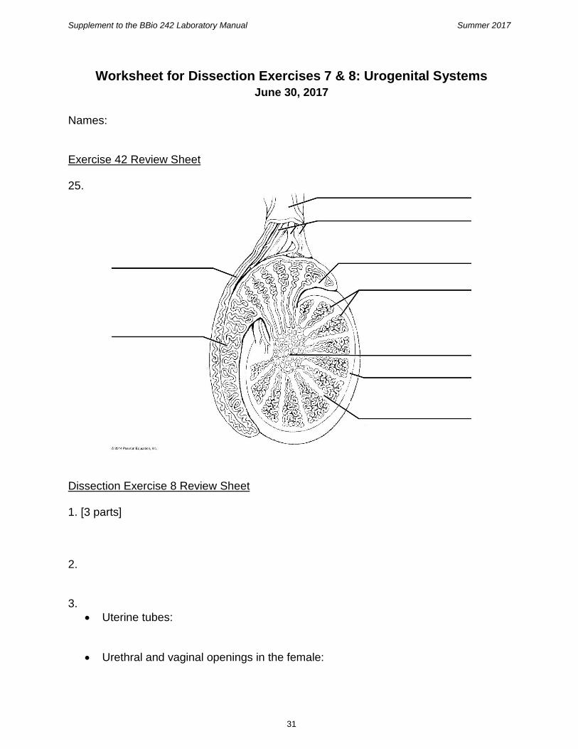
Names: Exercise 42 Review Sheet 25.

Dissection Exercise 8 Review Sheet 1. [3 parts] 2. 3.

• Uterine tubes:

• Urethral and vaginal openings in the female:


32

• Location of the penis: Additional questions 1. Does the urethra have any non-reproductive functions? If so, what? 2. List the structures, in order, through which a sperm passes up to and including the point where it fertilizes an oocyte. 3. List the structures, in order, through which an oocyte passes up to and including implantation. 4. What is an ectopic pregnancy, and where does it usually occur? Identification of structures 5. Instructor’s initials to indicate successful identification of pig structures: _________ 6. Instructor’s initials to indicate successful identification of sheep structures: _________

Metacognition


Why?


33

Exercise 29: Blood

July 3, 2017 Goals

• Observe general properties of plasma (Activity 1).

• Microscopically examine your own blood (Activities 2-3).

• Measure hematocrit and hemoglobin concentration (Activities 4-5).

• Measure the time it takes blood to clot (Activity 6).

• Perform ABO blood typing (Activity 7). Safety Come to lab dressed appropriately: long hair under control, long pants or long skirt, shoes that fully protect the feet. Note the “ALERT: Special precautions when handling blood” section on page 424. You will be handling (small amounts of) your own blood, so these precautions apply to you! For UW-Bothell labs, any sharp objects contaminated with blood (used lancets, used microscope slides) should go in the red biohazard sharps container. Any non-sharp bloody material (cotton balls, paper, swabs, toothpicks) should go into regular biohazardous waste (an autoclave bag). We do not use bleach for the disposal of these items, despite what the lab manual says. Instructions Perform the following activities. Record all data and answer all questions within each activity, with the exceptions noted below.

• Activity 1: Determining the Physical Characteristics of Plasma

• Activity 2: Examining the Formed Elements of Blood Microscopically o Collect and use your own blood. Carefully follow the staining instructions.

• Activity 3: Conducting a Differential WBC Count o You do not need to do a formal count of the white blood cells; just scan

your slide and determine which WBC types are most common. Note that the different types of WBCs can be distinguished by (A) the shape of their nuclei and (B) the presence or absence or granules in the cytoplasm.

• Activity 4: Determining the Hematocrit o Start with this activity so that the centrifuge can spin all samples at once. o We will use cow blood; shake it up before using it! o Note which centrifuge slot your tube goes into.

• Activity 5: Determining Hemoglobin Concentration o Use the Tallquist method, not a hemoglobinometer.

• Activity 6: Determining Coagulation Time o This doesn’t always work well, but give it a shot, using a “good bleeder.”

• Activity 7: Typing for ABO and Rh Blood Groups


34

o Do ABO typing but not Rh typing.


35

Worksheet for Exercise 29: Blood Due July 3, 2017

Names: Activity 1: Determining the Physical Characteristics of Plasma pH of Plasma [1 part] Color and Clarity of Plasma [2 parts] Consistency [1 part]

Activity 2: Examining the Formed Elements of Blood Microscopically [nothing to fill in] Activity 3: Conducting a Differential WBC Count Which WBC type(s) appear(s) to be most common in your blood? Activity 4: Determining the Hematocrit Show your calculations and your results for % RBC, % WBC, and % plasma. Activity 5: Determining Hemoglobin Concentration _____ g/100 mL of blood _____% Hb Activity 6: Determining Coagulation Time [2 parts]


36

Activity 7: Typing for ABO and Rh Blood Groups Clumping with anti-A antibody? Clumping with anti-B antibody? (Skip anti-Rh part.) Blood type = Review Sheet 1. [2 parts] 2. 6. 14. 15. [2 parts] 17. [5 parts] 18. [2 parts] 19. [2 parts]

Metacognition


Why?


37

Exercise 30: Anatomy of the Heart

July 5, 2017

Goals

• Identify and name the chambers, valves, and major blood vessels of the heart (Activity 1 and Dissection).

• Trace the flow of blood into, through, and out of the heart (Activity 2).

• Understand the major differences between the pulmonary and systemic circuits. Safety Come to lab dressed appropriately: long hair under control, long pants or long skirt, shoes that fully protect the feet. Instructions Perform the following activities, answering all questions within each activity aside from the exceptions noted below.

• Activity 1: Using the Heart Model to Study Heart Anatomy o Use the model hearts embedded in the large human torso models. Focus

on the following structures: ▪ 4 chambers (what are their names?) ▪ 4 valves (what are their names?) ▪ chordae tendinae ▪ superior and inferior venae cavae (plural of vena cava) ▪ pulmonary trunk/arteries ▪ pulmonary veins ▪ aorta

• Activity 2: Tracing the Path of Blood Through the Heart o You may find this easier to do with a light-gray version of 11th Marieb

Figure 30-2b, such as that shown below.

• Activity 3: Using a Heart Model to Study Circulation o We will not examine the cardiac circulation in detail. Find the left coronary

artery, right coronary artery, and coronary sinus on the human torso model heart.

• Dissection: The Sheep Heart o We will use calf hearts rather than sheep hearts. o Review and continue to abide by the dissection tips listed in Dissection

Exercise 3. o To orient yourself, note that (A) the vena cava is generally of a darker color

than the other blood vessels and (B) the apex (the pointy bottom of the heart) is part of the left ventricle.

o The aorta and pulmonary arteries can be hard to distinguish because they are sort of intertwined. You can cut the connective tissue in between them, then insert a blunt probe into them to determine the chambers to which they connect.


38

o You do not need to answer the questions following steps 2, 3, and 10. o Focus especially on the structures listed above (Activity 1), plus…

▪ brachiocephalic trunk (first branch off of the aorta) ▪ ductus arteriosus (prenatal) / ligamentum arteriosum (postnatal) ▪ foramen ovale (prenatal) / fossa ovalis (postnatal)

• should be near opening of coronary sinus o After you have finished, your instructor will verify a couple of randomly

chosen examples of cardiac anatomy.

The heart of a newborn, showing the ductus arteriosus and foramen ovale. Ao = aorta; IVC = inferior vena cava; LA = left atrium; LV = left ventricle; PA = pulmonary artery; RA = right atrium; RV = right ventricle; SVC = superior vena cava. Figure from the Royal Children’s Hospital, Melbourne, Australia.


39

Worksheet for Exercise 30: Anatomy of the Heart

Due July 5, 2017

Names: Activity 1: Using the Heart Model to Study Heart Anatomy [nothing to fill in]

Activity 2: Tracing the Path of Blood Through the Heart

Activity 3: Using a Heart Model to Study Circulation [nothing to fill in] Dissection: The Sheep Heart 6. [2 parts]


40

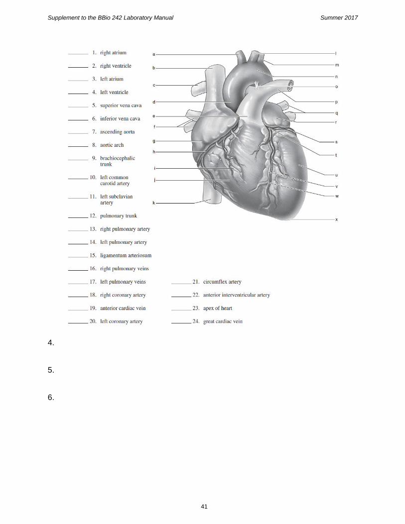
8. [3 parts] 9. 14. [6 parts] Instructor’s initials, indicating successful identification of cardiac structures: _______ Review sheet 1.


41

4. 5. 6.


42

8.

16.

Metacognition


Why?


43

Exercise 31: Conduction System of the Heart and Electrocardiography July 10, 2017

Goals

• Practice collecting an electrocardiogram (ECG or EKG) on a human volunteer (Activities 2-3).

• Use software to quantify the amplitude and duration of ECG components (Activities 4-5).

• Relate the electrical (muscle depolarization), mechanical (muscle contraction), and acoustical (heart sounds) events of the heart to each other (Activities 4-5.

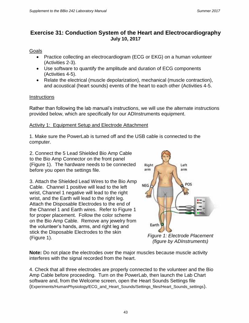
Instructions Rather than following the lab manual’s instructions, we will use the alternate instructions provided below, which are specifically for our ADInstruments equipment. Activity 1: Equipment Setup and Electrode Attachment 1. Make sure the PowerLab is turned off and the USB cable is connected to the computer. 2. Connect the 5 Lead Shielded Bio Amp Cable to the Bio Amp Connector on the front panel (Figure 1). The hardware needs to be connected before you open the settings file. 3. Attach the Shielded Lead Wires to the Bio Amp Cable. Channel 1 positive will lead to the left wrist, Channel 1 negative will lead to the right wrist, and the Earth will lead to the right leg. Attach the Disposable Electrodes to the end of the Channel 1 and Earth wires. Refer to Figure 1 for proper placement. Follow the color scheme on the Bio Amp Cable. Remove any jewelry from the volunteer’s hands, arms, and right leg and stick the Disposable Electrodes to the skin (Figure 1).

Figure 1: Electrode Placement

(figure by ADInstruments) Note: Do not place the electrodes over the major muscles because muscle activity interferes with the signal recorded from the heart. 4. Check that all three electrodes are properly connected to the volunteer and the Bio Amp Cable before proceeding. Turn on the PowerLab, then launch the Lab Chart software and, from the Welcome screen, open the Heart Sounds Settings file (Experiments/HumanPhysiology/ECG_and_Heart_Sounds/Settings_files/Heart_Sounds_settings).


44

Activity 2: Resting ECG 1. Have the volunteer assume a relaxed position. 2. Start recording. Add a comment with “Resting ECG.” Record the ECG for one minute. 3. Save your data when you are finished recording. Do not close the file. Activity 3: ECG and Phonocardiography In this exercise, you will use a Cardio Microphone placed over the chest wall to record the heart sounds, which allows the heart sounds to be displayed graphically in real time. (Note: We have stethoscopes if you want to listen directly as well.) 1. Connect the Cardio Microphone to Input 1 on the front panel of the PowerLab (Figure 2). The hardware needs to be connected before you open the settings file. 2. Open the settings file “Phonocardiography Settings” from the Experiments tab in the Welcome Center. It will be located in the folder for this experiment.

Figure 2: Equipment Setup for PowerLab 26T (figure by ADInstruments)

3. Have the volunteer place the Cardio Microphone on the left side of the chest against the skin. 4. Start recording. Move the Cardio Microphone to get the best signal possible. When ready, Stop recording, and tape down the Cardio Microphone. Note: It is important to tape down the Cardio Microphone instead of holding it as the hand introduces considerable noise into the recording. 5. Have the volunteer sit in a relaxed position, facing away from the monitor. Remind the volunteer not to move during the recording. 6. When ready, Start recording. Record for 15 seconds, and Stop. Save your data.


45

Activity 4: Analysis of ECG in a Resting Volunteer 1. Examine the data in the default window (Chart View). Use the View Buttons to set the horizontal compression to 20:1 or 10:1. Scroll through the data to observe the regularly occurring ECG cycles. 2. Use the Marker and Waveform Cursor to measure the amplitudes and durations of four P waves, QRS complexes, and T waves from the ECG trace.

• To measure the amplitudes, place the Marker on the baseline immediately before the P wave. Then move the Waveform Cursor to the peak of the wave.

• To measure the durations, place the Marker at the start of the wave or complex and position the Waveform Cursor at the end of the wave or complex.

3. Record these values in the table in your worksheet, and find the mean amplitude and duration for each phase of the cycle. 4. Use the View Buttons to set the horizontal compression to 10:1. Measure the time interval (in seconds) between three pairs of adjacent R waves using the Marker and Waveform Cursor (R-R time interval). For each interval, calculate the heart rate using the following equation:

ℎ𝑒𝑎𝑟𝑡 𝑟𝑎𝑡𝑒 (𝑏𝑒𝑎𝑡𝑠 𝑝𝑒𝑟 𝑚𝑖𝑛𝑢𝑡𝑒) =60

𝑅 − 𝑅 𝑡𝑖𝑚𝑒 𝑖𝑛𝑡𝑒𝑟𝑣𝑎𝑙 (sec)

5. Record these values in your worksheet. Activity 5: Analysis of ECG and Phonocardiography 1. Examine the data in the Chart View, and Autoscale, if necessary. Note the relationship between the R wave and the first heart sound. 2. Place the Marker on the R wave, and place the Waveform Cursor on the beginning of the first heart sound. Note the time between these two events as shown at right. 3. Repeat steps 1 and 2 for the T wave and its relationship with the second heart sound. 4. Record these values in the worksheet table.


46


47

Worksheet for Exercise 31 (Conduction System of the Heart and Electrocardiography)

Due July 10, 2017 Names: Activity 4: Analysis of ECG in a Resting Volunteer 1. Data table: ECG deflection waves 2. What does the P wave amplitude

represent? 3. How much does P wave amplitude vary from beat to beat? 4. Is this similar to the variation one would expect in skeletal muscle EMG recordings? Why or why not?

Amplitude

(mV)

Duration

(s)

P Wave 1

2

3

4

Mean

QRS

Complex

1

2

3

4

Mean


48

5. Data table: heart rate

R-R time interval (sec) Heart rate (beats/min)

Pair 1

Pair 2

Pair 3

Pair 4

Average heart rate:

Activity 5: Analysis of ECG and Phonocardiography 1. Data table: heart sounds

Start of QRS complex to start of first sound (sec)

Start of T wave to start of second sound (sec)

2. What do the sounds in the phonocardiograph represent? 3. Why do the heart sounds occur shortly after the start of the QRS complex and the start of the T wave, respectively? Metacognition


Why?


49

PhysioEx 6: Cardiovascular Physiology Due July 17, 2017

Goals

• Compare and contrast the action potential of a cardiac muscle cell with that of a typical neuron (Activity 1).

• Compare and contrast the refractory period of a cardiac muscle cell with that of a typical neuron (Activity 1).

• Contrast the effects of the sympathetic nervous system and parasympathetic nervous system on the heart (Activities 2 and 4).

Instructions Please complete Activities 1-2 and 4-5 of PhysioEx Exercise 6, found on pages PEx-93 through PEx-104 of your lab manual (toward the back).

• Activity 1: Investigating the Refractory Period of Cardiac Muscle

• Activity 2: Examining the Effect of Vagus Nerve Stimulation

• Activity 4: Examining the Effects of Chemical Modifiers on Heart Rate

• Activity 5: Examining the Effects of Various Ions on Heart Rate Follow the instructions given for the previous PhysioEx assignment (PhysioEx 4: Endocrine System Physiology). You do not need to answer the questions shown in the lab manual or online; instead, you will use Canvas to submit a brief report for each activity that includes the following sections: Experiment, Hypothesis, Results (both text and key tables or graphs), Conclusion.


50

Exercise 33: Human Cardiovascular Physiology: Blood Pressure and Pulse Determinations

July 19, 2017 Goals

• Practice taking pulses by hand and listening to heart sounds (Activities 1-2).

• Practice taking blood pressure readings (Activity 5).

• Investigate post-exercise pulse rate as an indicator of physical fitness (Activity 7). Instructions Perform the following activities, answering all questions within each activity aside from any exceptions noted below.

• Activity 1: Auscultating Heart Sounds

• Activity 2: Palpating Superficial Pulse Points

• Activity 5: Using a Sphygmomanometer to Measure Arterial Blood Pressure Indirectly

• Activity 7: Observing the Effect of Various Factors on Blood Pressure and Heart Rate

o Only do the Exercise portion of this activity (Harvard step test). Use the wood benches outside the lab, which are 17 inches high.

o Only record pulse data, not blood pressure data. o The lab manual’s formula for calculating the index of physical fitness is

confusing. Use the one provided in the worksheet (below) instead.


51

Worksheet for Exercise 33 (Human Cardiovascular Physiology: Blood Pressure and Pulse Determinations)

Names:

Activity 1: Auscultating Heart Sounds

3. [2 parts]

4.

Activity 2: Palpating Superficial Pulse Points

[7 parts]

Activity 5: Using a Sphygmomanometer to Measure Arterial Blood Pressure Indirectly

4.

5.

6.

Activity 7: Observing the Effect of Various Factors on Blood Pressure and Heart Rate

Each member of your group should try the step test.

Name

Resting heart rate (beats per minute)

Exercise duration (up to 300 sec)

Heart-beats, 1:00-1:30 post-exercise



Index of physical fitness*

Interpretation of index (see p. 501)

* 𝐼𝑛𝑑𝑒𝑥 =100∗(𝑒𝑥𝑒𝑟𝑐𝑖𝑠𝑒 𝑑𝑢𝑟𝑎𝑡𝑖𝑜𝑛 𝑖𝑛 𝑠𝑒𝑐𝑜𝑛𝑑𝑠)

2∗(𝑠𝑢𝑚 𝑜𝑓 𝑝𝑜𝑠𝑡−𝑒𝑥𝑒𝑟𝑐𝑖𝑠𝑒 𝑝𝑢𝑙𝑠𝑒 𝑐𝑜𝑢𝑛𝑡𝑠)


52

Supplement to Activity 7:

Which is a better indicator of fitness, resting heart rate or post-exercise heart rate?

It should make sense that the lower your heart rate is after a standardized exercise, the fitter you probably are. However, fitter people also tend to have lower resting heart rates than unfit people. Can we just use resting heart rate as an indicator of fitness, and skip the step test altogether? In a previous lab taught at UW-Seattle, students did a step test and then later a timed 1-mile run. Below are graphs showing correlations between resting heart rate and mile run performance, and between post-exercise heart rate and mile run performance.

Based on these data, which heart rate – at rest, or after the step test – is a better predictor of 1-mile run time? Explain.


53

Review Sheet

1.

2. [3 parts]


54

3. [10 parts] 5. [2 parts]


55

7. 1. ___________________ 2. ___________________ 3. ___________________ 4. ___________________ 5. ___________________ 6. ___________________ 7. ___________________ 9. [3 parts] 20. 21. [3 parts] 22. 23. [2 parts]

Metacognition


Why?


56


57

Exercise 36 and Dissection Exercise 5: Anatomy of the Respiratory System

July 24, 2017

Goals

• Learn gross and microscopic anatomy of the gas-conduction and gas-exchange sections of the respiratory system.

• Appreciate how the structures of these sections support their respective functions. Safety Come to lab dressed appropriately: long hair under control, long pants or long skirt, shoes that fully protect the feet. Exercise 36, Activity 1: Identifying Respiratory System Organs Using the lab manual pictures and our human torso model, find the following structures:

• Upper respiratory system o Hard palate (which bones form this?) and soft palate o Pharynx (throat): note the 3 parts (don’t need to remember the names) o Larynx o Epiglottis

• Lower respiratory system o Trachea o Esophagus o Right and left main (primary) bronchi o Terminal bronchioles o Alveoli o Lungs o Heart o Respiratory muscles: diaphragm and intercostals (2 layers)

Also, perform the larynx palpation described toward the end of page 538. Exercise 36, Activity 2: Demonstrating Lung Inflation in a Sheep Pluck We will use a pluck from a calf, not a sheep. Exercise 36, Activity 3: Examining Prepared Slides of Trachea and Lung Tissue We do not have pathological lung slides, so just look at the slides of normal trachea (look especially for the pseudostratified ciliated columnar epithelium and hyaline cartilage) and normal lung tissue. Dissection Exercise 5: Dissection of the Respiratory System of the Fetal Pig


58

Review and continue to abide by the dissection tips listed in Dissection Exercise 3. Look for the structures listed above (under Exercise 36, Activity 1). Also, see if you can find the phrenic nerve and vagus nerve, which appear as white bands. You do not need to do Activity 2 (Viewing Fetal Lung Tissue Under a Dissecting Microscope).


59

Worksheet for Exercise 36 and Dissection Exercise 5: Anatomy of the Respiratory System

Due July 24, 2017 Names: Exercise 36, Activity 3 How is your trachea slide similar to and/or different from Figure 36.6b? How is your lung tissue slide similar to and/or different from Figure 36.7b? Exercise 36 Review Sheet 4. [2 parts] 9. 11. [2 parts] 13. 16. [2 parts]


60

Dissection Exercise 5 Activity 1, #3: Activity 1, #8: Dissection Exercise 5 Review 1. 2. Instructor’s initials, indicating successful identification of respiratory structures: ________

Metacognition


Why?


61

PhysioEx 7: Respiratory System Mechanics Due August 1, 2017

Goals

• Measure respiratory volumes such as tidal volume (TV or VT), Residual Volume (RV), Forced Vital Capacity (FVC), and Forced Expiratory Volume in 1 second (FEV1) (Activity 1).

• Determine how emphysema and asthma affect normal respiratory measurements (Activity 2).

• Explain how surfactant affects lung function (Activity 3).

• Explain how negative intrapleural pressure keeps the lungs inflated (Activity 3).

Instructions Please complete Activities 1-3 of PhysioEx Exercise 7, found on pages PEx-105 through PEx-117 of your lab manual (toward the back).

• Activity 1: Measuring Respiratory Volumes and Calculating Capacities

• Activity 2: Comparative Spirometry

• Activity 3: Effect of Surfactant and Intrapleural Pressure on Respiration Follow the instructions given for previous PhysioEx assignments. You do not need to answer the questions shown in the lab manual or online; instead, you will use Canvas to submit a brief report for each activity that includes the following sections: Experiment, Hypothesis, Results (with both text and key tables or figures), Conclusion.


62

Exercise 37: Respiratory System Physiology (adapted from a BBio 352 lab by Jeff Jensen)

July 26, 2017

Goals

• Collect spirometric data (Activities 3 and 5).

• Measure respiratory parameters such as tidal volume (TV or VT), Residual Volume (RV), Forced Vital Capacity (FVC), and Forced Expiratory Volume in 1 second (FEV1) (Activities 4 and 6).

• Explain how spirometry might be used to distinguish between obstructive lung disease and restrictive lung disease.

Background Many important aspects of lung function can be determined by measuring airflow and the corresponding changes in lung volume. In the past, this was commonly done by breathing into a bell spirometer, in which the level of a floating bell tank gave a measure of changes in lung volume. Flow, F, was then calculated from the slope (rate of change) of the volume, V (F = dV/dt). More conveniently, airflow can be measured directly with a pneumotachometer (from Greek roots meaning “breath speed measuring device”). The PowerLab pneumotachometer is shown in Figure 1. Figure 1: The PowerLab Pneumotachometer. All figures for this lab are by ADInstruments.

Several types of flow measuring devices are available; the one you will use today is a “Lilly” type that measures the difference in pressure on either side of a mesh membrane with known resistance. This resistance gives rise to a small pressure difference proportional to flow rate. Two small plastic tubes transmit this pressure difference to the Spirometer Pod, where a transducer converts the pressure signal into a changing voltage that is recorded by the PowerLab and displayed in the Flow channel of LabChart (the top/red channel of Figure 8 below). The volume is then calculated from the flow. Specifically, volume is the area under the flow-time curve, i.e., the integral of flow over time (V = ∫ F dt).


63

A complication in the volume measurement is caused by differences between inhaled air (which starts off at the temperature of the environment) and exhaled air (which is at body temperature). Gas expands with warming; therefore, you will breathe out a larger volume of air even though you are not breathing out more molecules of air. The volume of air expired can also be increased by humidification (adding water vapor), which happens in the alveoli. Computer software corrections can correct the data to show what it would look like at constant temperature and humidity. Spirometry allows many components of pulmonary function to be visualized, measured, and calculated (Figure 2). Respiration consists of inspiration followed by expiration, repeated over and over. During one respiratory cycle, a volume of air is drawn into and then expired from the lungs; this volume is the tidal volume (TV or VT). In normal ventilation, the breathing frequency (ƒ) is approximately 15 respiratory cycles per minute. This value varies with the level of activity. The product of ƒ and TV is the expired minute volume (VE), the amount of air exhaled in one minute of breathing. This parameter also changes according to the level of activity. Even when someone exhales completely, there is still air left in the lungs. This leftover air is the residual volume (RV), which cannot be measured by spirometry.

Figure 2. Lung Volumes and Capacities. EC = Expiratory Capacity; ERV = Expiratory Reserve Volume; FRC = Functional Residual Capacity; FVC = Functional Vital Capacity; IC = Inspiratory Capacity; IRV = Inspiratory Reserve Volume; RV = residual volume; TLC = total lung capacity; VC = vital capacity; VT = tidal volume. Overview of Instructions For this lab, we will follow the alternative instructions below, designed for our ADInstruments equipment. Please work in groups of 3 or 4. Make sure everyone has a job; for example, one person could be reading aloud from the paper protocol, another could be running the computer, another could be the experimental subject, and another could be supervising completion of the worksheet.


64

If you are suffering from a respiratory infection, do not volunteer for this experiment. The instructions below are lengthy, but the overall goal is simple: to calculate respiratory parameters like those shown in Figure 2 above (and as you’re doing in PhysioEx Exercise 7). Note that Figure 2 shows volumes (in units of, say, L), which must be calculated from flow rates (in units of, say, L/s) – which will be displayed in the bottom and top channels of your screen, respectively, as shown in Figure 8. Activity 1: Equipment Setup 1. Make sure the PowerLab is turned off and the USB cable is connected to the computer. 2. Connect the Spirometer Pod to Input 1 on the front panel of the PowerLab (Figure 3). Turn on the PowerLab. Note: Since the Spirometer Pod is sensitive to temperature and tends to drift during warm-up, it is recommended the PowerLab (and therefore the Spirometer Pod) is turned on for at least 10 minutes before use. To prevent temperature drift, place the Spirometer Pod in a shelf or beside the PowerLab, away from the PowerLab power supply to avoid heating. 3. Connect the two plastic tubes from the Respiratory Flow Head to the short pipes on the back of the Spirometer Pod. Attach Clean-bore Tubing, a Filter, and a Mouthpiece to the Flow Head (Figure 3). Note: A clean Mouthpiece and Filter should be supplied for each volunteer. The Mouthpiece can be cleaned between uses with a suitable disinfectant. Figure 3: Equipment Setup for PowerLab 26T.


65

Activity 2: Familiarize Yourself with the Equipment In this activity, you will learn the principles of spirometry and how integration of the flow signal gives a volume. Calibrating the Spirometer Pod The Spirometer Pod must be calibrated before starting this exercise. The Flow Head must be left undisturbed on the table during the zeroing process. 1. Launch LabChart and open the settings file “Airflow and Volume Settings” from the Experiments/HumanPhysiology/Respiratory Airflow & Volume/Settings folder. 2. Select Spirometer Pod from the Channel 1 Channel Function pop-up menu. Make sure the Range is 500 mV and the Low Pass is 10 Hz; then select Zero. When the value remains at 0.0 mV, have the volunteer breathe out gently through the Flow Head, and observe the signal (Figure 4). If the signal shows a downward deflection (it is negative), you can return to the Chart Window. If the signal deflects upward, you need to invert it. Click the Invert checkbox once. Click OK. Figure 4: Spirometer Pod Dialogue Box with Downward Deflection.

Note: The signal can also be inverted by reversing the orientation of the Flow Head or by swapping the connections to the Spirometer Pod. The Invert checkbox is more convenient. Using the Equipment 3. Have the volunteer put the Mouthpiece in their mouth and hold the Flow Head carefully with both hands. The two plastic tubes should be pointing upward. 4. Put the nose clip on the volunteer’s nose. This ensures that all air breathed passes through the Mouthpiece, Filter, and Flow Head (Figure 5).


66

5. After the volunteer becomes accustomed to the apparatus and begins breathing normally, you are ready to begin. Figure 5: Proper Positioning of the Flow Head.

6. Start recording. Have the volunteer perform a full expiration and then breathe normally. Record the volunteer’s tidal breathing for one minute. At the end of one minute, have the volunteer perform another full expiration. Observe the data being recorded in the “Flow” (top) channel. Stop recording. The volunteer can stop breathing through the Flow Head and can remove the Nose Clip. Setting Up the Spirometry Extension The Spirometry Extension processes the raw voltage signal from the Spirometer Pod, applies a volume correction factor to improve accuracy, and displays calibrated Flow (L/s) and Volume (L) traces. The trace you recorded in the exercise above will provide reference points for the Spirometry Extension that allow it to correct the raw traces. 7. Drag across the Time axis at the bottom of the Chart Window to select the data you recorded. For volume correction (below) to work properly, you should select a region consisting of full exhalation for the first third (approximately), inhalation for the second third, and full exhalation again for the last third. Select Spirometry Flow from the Channel 1 Channel Function pop-up menu. Make sure the settings are the same as those in Figure 6. Click OK. 8. Select Spirometry Volume from the Channel 2 Channel Function pop-up menu. Make sure Channel 1 is selected in the Spirometry Flow Data pop-up menu. Click the Apply Volume Correction checkbox to turn it on. Then select Apply to allow the extension to use the volume correction ratio that is has calculated from your data (Figure 7). The volume correction ratio should be between 1.02 and 1.12; if it isn’t, check with your instructor. The Chart Window should now appear with calculated volume data in Channel 2 (lower channel).


67

Figure 6: Spirometry Flow Dialogue Box. (Ours may look slightly different.)

Figure 7: Spirometry Volume Dialogue Box. (Ours may look slightly different.)

9. Select Set Scale from the Scale pop-up menu in the Amplitude axis for the “Flow” channel (look for the triangle way in the upper left). Select “Set Scale,” then make the top value 15 L/s and the bottom value -15 L/s. Click OK. Understanding the Importance of Volume Correction 10. Drag across the Time axis to select data from both channels, and open the Zoom View of the Window menu (at top, above “Window”). Note the relation between Flow and Volume. When the flow signal is positive (inspiration), Volume rises; when the flow is negative (expiration), Volume falls. 11. In Zoom View, find part of the recording where the flow is zero. Note that at this time, Volume does not change (the line is horizontal) because if there is no flow in or out, the volume of air in the lungs is staying the same. 12. The volume trace is calculated by the extension in such a way that the displayed volumes at the end of the two full expirations are equal. In subsequent recordings, the volume correction is unlikely to be exact – you will notice a tendency for the volume to drift, typically 1-2 L over 1-2 minutes. To see the effect of having no correction, turn off the Volume Correction checkbox in the Spirometry Volume dialog box, and examine the data trace. Remember to turn it back on again afterward. 13. Save your data. Do not close the file. Activity 3: Lung Volumes and Capacities In this exercise, you will examine the respiratory cycle and measure changes in flow and volume. 1. Have the volunteer face away from the monitor and read. This will prevent the volunteer from consciously controlling their breathing during the exercise.


68

2. When ready, Start recording. After two seconds, have the volunteer replace the Nose Clip and breathe normally into the Flow Head. Record normal tidal breathing for one minute. Add a comment with “normal tidal breathing” to the data trace. 3. After the tidal breathing period (at the end of a normal tidal expiration), ask the volunteer to inhale as deeply as possible and then exhale as deeply as possible. Afterwards, allow the volunteer to return to normal tidal breathing for at least three breaths. Stop recording when finished. 4. Position the cursor at the end of the deep breath. Right-click and select Add Comment. Add the comment “lung volume procedure” at the cursor position. 5. Save your data. Do not close the file. Activity 4: Analysis of Lung Volumes and Capacities Data 1. Examine the normal tidal breathing data in the Chart Window, and Autoscale, if necessary. Calculate how many breaths there are in a one-minute period (BPM). Record RR/min in Table 1 of your worksheet. 2. Determine the volume of a single tidal inspiration by placing the Marker at the start of a normal tidal inspiration and placing the Waveform Cursor at the peak (Figure 8). The value shown in the Range/Amplitude display for Channel 2 is the tidal volume (VT or VT) for that breath. Record this value in Table 1. Figure 8: Positioning the Marker (M) and Waveform Cursor (+) to measure tidal volume.

3. Use the values for tidal volume and the number of breaths observed over a one minute period to calculate the expired minute volume (VE). Use the following equation:


69

VE = RR x VT (L/min) 4. Find the “lung volume procedure” comment in your data trace. (You should be able to find it in a pull-down menu of comments.) Repeat steps 2-3 to determine the inspiratory reserve volume (IRV) (Figure 9) and expiratory reserve volume (ERV) (Figure 10; refer back to Figure 2 for definitions of volumes).

Note: The Marker should be placed at the peak of a normal tidal inspiration for IRV, and it should be placed at the start (trough) of a normal tidal inspiration for ERV.

5. Calculate the inspiratory capacity (IC) using the following equation:

IC = VT + IRV (L) 6. Calculate the expiratory capacity (EC) using the following equation:

EC = VT + ERV (L) Figure 9: Positioning the Marker (M) and Waveform Cursor (+) to Measure Inspiratory Reserve Volume (IRV).

Figure 10: Positioning the Marker (M) and Waveform Cursor (+) to Measure Expiratory Reserve Volume (ERV).


70

7. Referring to the Appendix below, use the tables provided to determine the volunteer’s predicted vital capacity (VC). The predicted value varies according to the volunteer’s sex, height, and age. 8. Calculate the volunteer’s measured VC using the experimentally derived values for IRV, ERV, and VT. Use the following equation:

VC = IRV + ERV + VT (L) 9. Residual volume (RV) is the volume of gas remaining in the lungs after a maximal expiration. The RV cannot be determined by spirometric recording. Using the following equation, determine the predicted RV value for the volunteer:

RV = predicted VC x 0.25 (L) 10. The total lung capacity (TLC) is the sum of the vital capacity and residual volume. Calculate the predicted TLC for the volunteer using the following equation (use the measured VC rather than the predicted one):

TLC = VC + RV (L)

11. Functional residual capacity (FRC) is the volume of gas remaining in the lungs at the end of a normal tidal expiration. Use the following equation:

FRC = ERV + RV (L) Activity 5: Pulmonary Function Tests In this exercise, you will measure parameters of forced expiration that are used in evaluating pulmonary function. 1. If necessary, zero the Spirometer Pod again, using the same procedure as before (Activity 2, step 2. Remember to leave the Flow Head undisturbed during the process. 2. Have the volunteer put on the Nose Clip and breathe normally into the Flow Head. 3. Start recording. Add a comment with the volunteer’s name. 4. Prepare a comment with “forced breathing.” Have the volunteer breathe normally for 30 seconds; then ask the volunteer to inhale maximally and then exhale as forcefully and fully as possible until no more air can be expired. Add the comment. After a few seconds, the volunteer should let their breathing return to normal. Stop recording. Do not close the file. 5. Repeat steps 3-4 twice more, so that you have three separate forced breath recordings (Figure 11). Save your data. Do not close the file.


71

Figure 11: Sample Data of Forced Breaths.

Activity 6: Analysis of Pulmonary Function Test Data 1. In the last data block of your LabChart recording for this exercise, move the Waveform Cursor to the maximal forced inspiration in “Flow.” The absolute value displayed in the Range/Amplitude display is the peak inspiratory flow (PIF). Multiply the value by 60 to convert from L/s to L/min. 2. From the flow data trace, measure the peak expiratory flow (PEF) for the forced expiration. Multiply the value by 60 to convert from L/s to L/min. Disregard the negative sign. 3. To calculate the forced vital capacity (FVC), place the Marker on the peak inhalation of “Volume,” and move the Waveform Cursor to the maximal expiration (Figure 15). Read off the result from the Range/Amplitude display, disregarding the delta symbol and negative sign. 4. Return the Marker to its box. To measure forced expired volume in one second (FEV1), place the Marker on the peak of the volume data trace, move the Waveform Cursor to a time 1.0 s from the peak, and read off the volume value. If you find it hard to adjust the mouse position with enough precision, a time value anywhere from 0.96 s to 1.04 s gives enough accuracy. Disregard the delta symbol and negative sign. 5. Repeat this analysis until all three forced breaths have been analyzed. 6. Calculate the percentage ratio of FEV1 to FVC for your experimental and Spirometry Extension results. Use the maximum values of FEV1 and FVC, and use the following equation:

(FEV1 / FVC) x 100 (%)


72

7. Record your values in Table 2 of the worksheet. Appendix: Predicted Vital Capacities for Males and Females

Table 1. Predicted Vital Capacities (in liters) for males, according to height (in centimeters) and age.

Table 2. Predicted Vital Capacities (in liters) for females, according to height (in centimeters) and age. Source: The Johns Hopkins Pulmonary Function Laboratory equations for pulmonary function (http://www.hopkinsmedicine.org).


73

Worksheet for Exercise 37 (Respiratory System Physiology) Due July 26, 2017

Names: Table 1: Lung volumes and capacities

Respiratory Parameter Value, including proper units

Respiratory Rate (RR)

Expired Minute Volume (VE)

Tidal Volume (VT)

Inspiratory Reserve Volume (IRV)

Inspiratory Capacity (IC)

Expiratory Reserve Volume (ERV)

Expiratory Capacity (EC)

Vital Capacity (VC)

Predicted (from table in appendix)

Measured

Residual Volume (RV), estimated

Total Lung Capacity (TLC)

Functional Residual Capacity (FRC)


74

Table 2: Pulmonary function tests

Respiratory Parameter Value, including proper units

Peak Inspiratory Flow

(PIF)

1st forced breath:

2nd forced breath:

3rd forced breath:

Peak Expiratory Flow

(PEF)

1st forced breath:

2nd forced breath:

3rd forced breath:

Forced Vital Capacity

(FVC) – circle the

maximum value

1st forced breath:

2nd forced breath:

3rd forced breath:

Forced Expired Volume in

One Second (FEV1) –

circle the maximum value

1st forced breath:

2nd forced breath:

3rd forced breath:

(FEV1 / FVC) x 100

(assume FEV1 and FVC to

be the max values above)

Study Questions 1. Explain why RV cannot be determined by ordinary spirometry (like what we did today). 2. How did the subject’s measured VC compare to the VC predicted according to his/her age and height? 3. A typical FEV1/FVC is ≥80%. Does your subject have a normal FEV1/FVC?


75

4. Explain the basic difference between obstructive lung disease and restrictive lung disease. 5. Is a lower-than-normal VC most consistent with obstructive lung disease or restrictive lung disease? 6. Is a lower-than-normal FEV1/FVC (<80%) most consistent with obstructive lung disease or restrictive lung disease?

Metacognition


Why?


76


77

Exercise 38 and Dissection Exercise 6:

Anatomy of the Digestive System

July 31, 2017

Goal

• Identify and name key anatomical structures responsible for the digestion of food and excretion of waste.

Exercise 38, Activity 1: Organs of the Alimentary Canal You do not need to find all of the structures mentioned in this activity. Using the human torso model and figures in your lab manual, concentrate on the ones listed below. In finding those, you should use the following non-digestion/excretion structures as “landmarks” that you have seen in previous labs: diaphragm, kidneys, spleen.

• Anus

• Bile duct

• Cecum

• Colon (large intestine): ascending, transverse, descending

• Epiglottis

• Esophagus

• Gall bladder

• Liver

• Pancreas

• Parotid gland (a salivary gland)

• Rectum

• Small intestine: duodenum, jejunum, ileum

• Stomach, with pyloric sphincter

• Teeth

• Ureter

• Urethra

• Urinary bladder Exercise 38, Activities 2-4: Histology of the Digestive System Examine the following pre-prepared slides:

• Stomach (look for the 3 layers of muscle, simple columnar epithelium, gastric pits, chief cells, parietal cells, lumen)

• Small Intestine (look for microvilli, villi, simple columnar epithelium, lumen)

• Pancreas (look for endocrine and exocrine sections) In addition, see if you can find evidence of sphincters and transitions along the epithelium in a slide of the stomach-duodenum junction, ileo-cecal junction, or recto-anal junction.


78

Dissection Exercise 6, Activity 1: Identifying Oral Cavity Structures Review and continue to abide by the dissection tips listed in Dissection Exercise 3. Focus on finding the following structures:

• Epiglottis

• Esophagus

• Parotid gland (a salivary gland)

• Pharynx (throat)

• Tongue Dissection Exercise 6, Activity 2: Identifying Digestive Organs in the Abdominal Cavity Focus on finding the remaining structures listed above (under Exercise 38, Activity 1).


79

Worksheet for Exercise 38 and Dissection Exercise 6:

Anatomy of the Digestive System

Due July 31, 2017

Names: Exercise 38, Activities 2-4: Histology of the Digestive System How is your slide of the stomach similar to and/or different from Figure 38.6a-b? How is your slide of the small intestine similar to and/or different from Figure 38.9a? In your slide of the pancreas, how do the endocrine cells differ from the exocrine cells? Exercise 38 Review Sheet 2. [2 parts] 20. Dissection Exercise 6 Review 1.


80

2.

Additional questions 1. Complete the following table.

Structure Main digestive function

Bile duct

Cecum

Colon (large intestine)

Gall bladder

Liver

Pancreas

Salivary glands

Small intestine

Stomach

2. Instructor’s initials, verifying identification of digestive system structures: ____


81

3. What part of today’s lab will be most important for you to review before the next test?

Why?


82


83

Exercise 39: Digestive System Processes: Chemical and Physical

August 2, 2017

Goals

• Observe the activity of protein-digesting and lipid-digesting enzymes (Activities 2-3).

• Learn about mechanisms by which the digestive system propels and mixes food (Activity 5).

Instructions In this lab, you will work in groups of 3 or 4. Each table should form a group. Each group will perform the following parts of the lab:

• Activity 2: Assessing Protein Digestion by Trypsin

• Activity 3: Demonstrating the Emulsification Action of Bile and Assessing Fat Digestion by Lipase

o Give a quick shake to the litmus cream before you use it.

• Group Challenge: Odd Enzyme Out

• Activity 5: Observing Movements and Sounds of the Digestive System The two main experiments are on protein digestion by trypsin (Activity 2) and fat digestion by lipase (Activity 3, step 3). Each experiment includes a 60-minute incubation step, so get these going before you do anything else. Then do the beginning of Activity 3 (emulsification of lipids by bile) and proceed to Activity 5. The antiquated abbreviation “gtt” used in your lab manual simply means “drops.” Note that 0.1 N HCl is highly acidic and therefore dangerous. Wearing gloves when handling it will decrease your dexterity, so please plan accordingly. This exercise includes the following tables for recording data: “Salivary Digestion of Starch”; “Trypsin Digestion of Protein”; “Pancreatic Lipase Digestion of Fats.” Ignore the table on Salivary Digestion of Starch, as we will not be doing that experiment. During lab, fill in your predictions for each tube of the other two tables into the modified versions of these tables found in the lab worksheet.


84


85

Worksheet for Exercise 39

(Digestive System Processes: Chemical and Physical)

Names: Activity 2: Protein Digestion by Trypsin

Tube no. 1T 2T 3T 4T 5T

Additives (3 drops each)

Trypsin, water

BAPNA, water

Trypsin (boil), then BAPNA

Trypsin, BAPNA

Trypsin, BAPNA

Incubation condition

37º C 37º C 37º C 37º C 0º C

Predicted color change?

Actual color change?

Explanation of protein digestion results (one paragraph or several bullet points):


86

Activity 3: Demonstrating the Emulsification Action of Bile and Assessing Fat Digestion by Lipase 2. In which tube has emulsification occurred?

Tube no. 1L 2L 3L 4L 5L 4B 5B Additives (5 drops each)

Lipase, water

Litmus cream, water

Lipase (boil), then litmus cream

Lipase, litmus cream

Lipase, litmus cream

Lipase, litmus cream, bile salts

Lipase, litmus cream, bile salts

Incubation condition

37º C 37º C 37º C 37º C 0º C 37º C 0º C

Predicted color change?

Actual color change?

Explanation of lipid digestion results (one paragraph or several bullet points): How are your test-tube digestion reactions similar to and different from what actually happens in your digestive tract? Try to think of 2 similarities and 2 differences. SIMILAR: DIFFERENT:


87

Group Challenge: Odd Enzyme Out

1. Which is the “odd enzyme”? Why is it the odd one out?




Activity 5: Observing Movements and Sounds of the Digestive System 2. 3. [2 parts] 4.


88

Review Sheet 1.

4.

Enzyme Organ producing it

Site of action Substrate(s) Optimal pH

Salivary amylase

Trypsin

Lipase (pancreatic)

5. Proteins: ______________________ Carbohydrates: ____________________ Fats: _________________________ and _______________________________ 12. [2 parts] Metacognition


Why?


89

Exercise 41: Urinalysis and ECF Regulation

August 7, 2017

Goals

• Test for abnormalities in urine color, pH, [glucose], [protein], and specific gravity, which may be symptoms of underlying disease.

• Investigate the regulation of extracellular fluid (ECF) volume by comparing urine volumes resulting from drinking water (hyposmotic to body fluids) or soup broth (isosmotic with body fluids).

Materials Outside the lab:

• Chicken broth

• Water

• Large cups, able to hold 20 fluid ounces (~600 milliliters) At each lab station:

• Urine specimen containers

• Disposable pipets

• Urine reagent strips

• pH strips

• Absorbent paper towel

• Urine collection containers At the central materials station:

• Hydrometer and jar

• Distilled or deionized water

• pH chart

• 2 marking pens

• Simulated urine specimens

• 10-mL graduated cylinders Lab overview For this exercise, we will NOT use the protocol in your lab manual; instead, we will follow the alternative directions below. There are two parts: ECF regulation, and physical and chemical analysis of urine (urinalysis). We will begin and end the lab with ECF regulation, and do urinalysis during the rest of the time. Background on regulation of ECF A core principle of physiology that we have revisited throughout the year is that of homeostasis. Mammals such as humans maintain homeostasis in part by regulating their extracellular fluid (ECF), the fluid found outside the body’s cells (such as the plasma


90

of blood). Two regulated aspects of ECF are its volume and its osmolarity; the body tries to keep both relatively constant. But which is regulated more tightly? To answer this question, we can do a simple experiment: challenge the body with a load of additional water (whose osmolarity is far below that of body fluids) or soup broth (whose osmolarity is similar to that of body fluids). Procedure for regulation of ECF 1. Immediately before lab, go to the bathroom and void your bladder to the best of your ability. 2. Sign up to drink either water or chicken soup broth. We will aim to have roughly equal numbers of students in the two groups. 3. Outside the lab, drink 20 fluid ounces (~600 milliliters) of water or soup broth. 4. Just before the end of the lab, pee again, measuring the volume of urine produced and reporting that volume to your instructor. If you have to pee more than once during the lab, please monitor each episode of urination and report the total urine volume to your instructor at the end. Background on urinalysis [provided by Carolina Biological Supply Company] Normally, urine consists of approximately 95% water and 5% dissolved solids such as urea and sodium chloride. Almost all substances found in urine also are found in blood, but at different concentrations. Some substances, such as glucose, have a threshold that must be exceeded before the substance is excreted in the urine. The presence of such substances in the urine usually indicates disease. Normal urine colors range from light yellow to amber, depending on the concentration of urochrome, the urinary pigment. Food, drugs, and disease can cause lighter or darker urine, as listed in Table 1. The pH of a solution is a measure of its free hydrogen ion (H+) concentration, which indicates acidity or alkalinity. Typically, the pH of normal urine is about 6, which is slightly acidic. Some foods and diseases that can affect urine pH are listed in Table 2.

Table 1: Urine color and possible causes

Color Diet Drugs Disease

Light yellow to amber Normal none None

Clear to light yellow Increased fluid intake Alcohol, phosphate, carbonate

Uncontrolled diabetes mellitus

Yellow orange to dark green

Carrots antibiotics Bilirubin from obstructive jaundice

Red to red brown Beets Laxatives Hemoglobin in in urine

Smoky red Beets Anticonvulsants Unhemolyzed red blood cells from urinary tract

Dark wine Beets Anti-inflammatory drugs Hemolytic jaundice


91

Brown black Rhubarb antidepressants Melanin pigment from melanoma

Brown Rhubarb Barbiturates Anemia or liver infections

Green Green food dyes diuretics Bacterial infection

Specific gravity is the density of a solution relative to that of water, which is 1.000. The specific gravity of normal urine ranges from 1.010 to 1.025; that is, normal urine is slightly denser than pure water. Specific gravity varies according to fluid intake and can be affected by disease. Glucose (sugar) should not be detected in normal urine; its presence usually indicates diabetes mellitus, a severe metabolic disorder caused by defective carbohydrate utilization. Glucose may also be present in the urine after a big meal or during times of emotional stress. A very small amount of protein is normally present in the urine. Any change in the color of a protein test strip indicates an elevated level of protein in urine. Diet and disease can affect protein levels in urine. For example, patients with severe anemia usually excrete protein in their urine.

Table 2: Abnormal urinalysis results and possible causes Possible causes

Test result Diet Disease

Low pH (<5) High protein diet; cranberry juice Uncontrolled diabetes mellitus

High pH (>8) Diet rich in vegetables; dairy products Severe anemia

Low specific gravity (<1.01) Increased fluid intake Severe renal damage

High specific gravity (>1.025) Decreased fluid intake; loss of fluids Uncontrolled diabetes mellitus; severe anemia

Glucose present (glycosuria) Large meal Uncontrolled diabetes mellitus

Protein present (proteinuria) High-protein diet Severe anemia

Procedure for urinalysis [provided by Carolina Biological Supply Company] In this activity, working in groups of two, you will perform five important tests routinely done in clinical urinalysis: color, pH, specific gravity, glucose, and protein. The Low, Normal, and High simulated urine samples are designed to produce results indicative of those characteristics. 1. Take three plastic urine specimen containers to the central materials station. Use a marking pen to label the containers Low, Normal, and High. Use the labeled graduated cylinders at the central materials station to transfer 10 milliliters of Low, Normal, and High Simulated Urine to the appropriate labeled containers. 2. Return to your lab station. Place the containers of simulated urine on the absorbent paper towel. Observe the samples, and record the color of each sample in your worksheet data table.


92

3. Use a pen or pencil to label one end of three of the pH test strips L, N, and H. 4. Holding the labeled end, dip the L strip into the Low sample. Shake off any excess liquid. Lay the pH strip in front of the Low sample on the absorbent paper towel. Repeat the process with the Normal (N strip) and High (H strip) samples. 5. Compare the color of the test strip to the pH color chart at the central materials station. In your data table, record the pH of each sample. 6. Label the plastic portion of three Urine Reagent strips L, N, and H, respectively. 7. Test each sample for glucose and protein using a Urine Reagent strip, as follows.

a. Observe the color of the test squares that are attached at one end of the urine reagent strip. The greenish square nearest the tip will be used for testing the glucose in the sample; the yellow square will detect protein in the sample. b. Dip the end of the strip with the test squares into the urine sample, then withdraw it. Run the end of the strip against the rim of the urine container to remove excess urine. c. Wait 30 seconds, then observe and record the color of the test squares.

• Green square: A negative result produces no color change, indicating normal or low urine glucose. A darkening of the square indicates a higher than normal urine glucose level; the darker the color, the higher the glucose level.

• Yellow square: A negative result produces no color change, indicating the absence of protein in the urine. A green or blue color indicates the presence of protein in the urine sample.

8. Calibrate the hydrometer, as follows. a. Rinse the urine hydrometer and jar thoroughly.

b. Use a clean pipet to fill the jar slightly more than half-full with distilled or deionized water. c. Insert the hydrometer as shown in Figure 1. The hydrometer should not touch the bottom of the jar. If it does touch, use a pipet to add water to the jar until the hydrometer floats. d. Read the water level on the hydrometer scale, and record the value in your data table. Units on the hydrometer scale are 1.000, 1.020, 1.040, and 1.060. If the measured value is not 1.000, the standard specific gravity of water, you will need to adjust your urine measurements to compensate. The calibration factor is


93

the value that must be added to or subtracted from the measurement to equal 1.000. e. Record the calibration factor for the hydrometer in your data table. f. Remove the hydrometer from the jar. Mark the level of the water remaining on the jar. You will use this line as the fill line when analyzing your samples. g. Empty the jar.

9. Measure the specific gravity of Simulated Urine Low. a. Rinse the urine hydrometer and jar thoroughly. b. Use a clean pipet to fill the jar to the fill line with the sample. c. Insert the hydrometer into the jar as shown in the figure. d. Read the fluid level on the hydrometer scale, and record the value in your data table. e. Add or subtract the calibration factor to or from your measurement. Record the adjusted value in your data table. 10. Repeat the specific gravity test for the Normal and High samples, and record the results in your data table.

Figure 1: Calibrating a hydrometer. Image from grapestompers.com.

11. Repeat the procedure for samples Unknown A and Unknown B. Analyze the color, pH, glucose, protein, and specific gravity of these samples, and record the results in your data table.


94


95

Worksheet for Exercise 41: Urinalysis and ECF Regulation

Due August 14, 2017

Names: ECF Regulation: Hypotheses and Predictions Consider two alternative hypotheses:

• A: The body regulates ECF volume more tightly than ECF osmolarity.

• B: The body regulates ECF osmolarity more tightly than ECF volume. To test these hypotheses, you will measure the volume of urine produced after drinking a large volume of water or soup broth. Note that drinking either fluid will alter ECF volume, but only the water will alter ECF osmolarity, since the osmolarity of the soup broth is similar to that of body fluids. 1. You urinate in part to get rid of excess ECF. The question here is, how much urine will be produced in response to each drink?

A. Predict how urine volume in the water group will compare with urine volume in the soup group if Hypothesis A is correct.

B. Predict how urine volume in the water group will compare with urine volume in the soup group if Hypothesis B is correct.

ECF Regulation: Raw Data 2. List the volume of urine produced by each member of the water group, including correct units: 3. List the volume of urine produced by each member of the soup group, including correct units:


96

ECF Regulation: Statistical Analysis 4. Mean ± standard deviation for water group: 5. Mean ± standard deviation for soup group: 6. Are these two sets of values significantly different from each other, according to an unpaired t-test, assuming unequal variances for the two groups? Report a p-value and explain what it means. Refer back to Exercise 27 (especially its appendix on statistics) if needed. ECF Regulation: Conclusion 7. Do your results more strongly support Hypothesis A or Hypothesis B? Explain. Urinalysis: Data Table 8.

Simulated Urine Samples

Urine Test Low Normal High Unknown A Unknown B

Color pH Glucose Protein Specific Gravity

Urinalysis: Study Questions 9. Explain why it is important to ask patients about their diet and medications when analyzing their urine.


97

10. Using Table 1 and Table 2, determine which disease(s), if any, may be indicated by the urine test results for Unknown A and Unknown B. Explain your reasoning. 11. In a clinical setting, urine is often examined under a microscope. What information about a patient’s health might be gained through this type of examination? Explain.

Metacognition


Why?


98


99

More Urinary System Physiology

August 9, 2017

Goals

• Use clinically relevant materials (blood and dialysis tubing) to simulate

glomerular filtration.

• Use beads and markers to create a model of glomerular filtration, tubular

reabsorption, and tubular secretion.

Materials

For Activity 1:

• Dialysis tubing

• String

• Scissors

• Animal blood

• Beaker containing 200 mL of deionized water

• Urinalysis strips

For Activity 2:

• Beads for each group (with preferred sizes):

o 1 large red

o 1 large white

o 2 large purple

o 5 small dark green

o 2 small light green

o 15 small orange

o 5 small yellow

o 25 small blue

o 15 small black

• Large sheets of paper (e.g., from a flip-chart)

• Petri dishes (2 per group)

• Pipe cleaners or string

• Markers of various colors (black, brown, red, blue, orange, purple, yellow,

green)

Overview

This lab is adapted from Chapter 31 (Physiology of the Urinary System) of Human

Anatomy & Physiology Laboratory Manual: Making Connections (2016) by Catharine C.


100

Whiting. It includes two activities: (1) demonstrating the function of the filtration

membrane and (2) simulating the events of urine production and urine concentration.

You will start with Activity 1 and then, when you finish step 5 and have to wait 30

minutes, start Activity 2.

Activity 1: Demonstrating the Function of the Filtration Membrane

In this activity, you will build a model using animal blood and dialysis tubing in order to

learn about the process of glomerular filtration. The dialysis tubing you will use, like a

filtration membrane, is a semipermeable membrane.

The substances that are able to pass out of the blood through the filtration membrane

(the dialysis tubing) will enter the “filtrate” (water), whereas those that are unable to pass

through the filtration membrane will remain in the blood. You will use urinalysis test

strips to test the filtrate for the presence of erythrocytes (RBCs), leukocytes (WBCs),

protein, and glucose.

1. Put on safety glasses and gloves.

2. Cut a 4-inch piece of dialysis tubing, and securely tie off one end of the tubing with a

piece of string.

3. Wet the other end of the tubing and rub it between your fingers to open it.

4. Fill the tubing about half-full with blood, and securely tie off the open end of the tubing

with another piece of string.

5. Place the tied-up “tube” in a beaker containing 200 mL of deionized water, and leave it

there for 30 minutes.

6. Predict which substances will be able to pass through the filtration membrane and

provide a rationale for your prediction.

7. After 30 minutes, remove the “tube” from the beaker.

8. Dip a urinalysis strip into the water and then remove it quickly. Follow the directions

on the side of the urinalysis strip bottle to determine the results for the four substances

(erythrocytes, leukocytes, protein, glucose).

Activity 2: Simulating the Events of Urine Production and Urine Concentration


101

Introductory Drawing & Labeling

For the three parts of this activity you will need a drawing of a simplified nephron (see

Figure 1) to help you visualize the movements of substances into and out of the nephron.

Create and adorn this drawing as described below.

a. Use red and black markers to redraw Figure 1 onto a large piece of blank paper. The

red glomerulus should be about the size of a petri dish.

b. Label the following structures: Bowman’s capsule (write “BC”), proximal tubule (PT),

loop of Henle (LH), distal tubule (DT), and collecting duct (CD).

c. Draw a dotted line through the nephron to indicate the boundary between the cortex

and the medulla. Label these two sides of the line.

d. Label the glomerulus (G), afferent arteriole (AA), and efferent arteriole (EA). (Note that

the depiction of peritubular capillaries and vasa recta is not anatomically correct; the

peritubular capillaries arise from efferent arterioles of cortical nephrons, whereas the

vasa recta arise from efferent arterioles of juxtamedullary nephrons.)

e. Draw a green box around the renal corpuscle. (Do filtration, reabsorption, and/or

secretion occur here?)

f. Draw an orange box around the renal tubule. (Do filtration, reabsorption, and/or

secretion occur here?)

g. Draw small black and brown circles in the interstitium of the medulla to represent

sodium ions (Na+) and chloride ions (Cl-), respectively. Use the circles to show the

interstitial concentration gradient.

h. Finally, separate a petri dish into its two halves. Label one half “blood” and the other

half “filtrate.” The different beads will represent different substances in the blood and

filtrate, as follows:

• large red bead = red blood cell

• large white bead = white blood cell

• large purple beads = plasma proteins

• small dark green beads = creatinine

• small light green beads = penicillin

• small orange beads = glucose


102

• small yellow beads = urea molecules

• small blue beads = water molecules

• small black beads = sodium and chloride ions

Figure 1: A simplified schematic view of a nephron and its blood supply. Figure taken from C.C. Whiting (2016).

Figure 2: Demonstrating glomerular filtration. Figure taken from C.C. Whiting (2016).

Part A: Glomerular Filtration in the Renal Corpuscle

In this part of the activity, you will demonstrate the movement of substances from the

blood of the glomerulus into the glomerular space of the glomerular capsule.

a. Using a piece of pipe cleaner or string, connect a plasma protein and the penicillin to

indicate that the two are typically bound together.

b. Fill the “blood” petri dish with the beads listed above. For now, include only 5 of the

(small, orange) glucose beads.

c. Move the “blood” dish into the afferent arteriole.

d. Move the “blood” dish into the renal corpuscle.

e. Demonstrate glomerular filtration. For substances that are freely filtered, move an

appropriate percentage of the corresponding beads (what percentage should that be?)

into the “filtrate” dish in the glomerular space, as shown in Figure 2. For substances that

are not in the filtrate under normal circumstances, leave all the beads in the “blood” dish

within the glomerulus.


103

Part B: Tubular Reabsorption into the Peritubular Capillary

In this part of the activity you will move the “blood” from the glomerulus into the efferent

arteriole and then into the peritubular capillaries surrounding the proximal tubule. You

will move the “filtrate” from the glomerular capsule into the proximal tubule.

a. Different solutes are reabsorbed to different extents by the proximal tubule. Out of

what is in the initial filtrate, nearly 100% of the glucose and organic nutrients get

reabsorbed; that figure is closer to 65% for water and inorganic ions (Na+, Cl-, K+, Ca2+,

etc.), ~50% for urea, and ~0% for creatinine. Move the beads in a way that reflects

these numbers.

b. Now consider a situation where there is three times the usual level of glucose in the

plasma. With the glucose beads, show whether/how the filtrate would be altered at the

end of filtration (Part A above) and at the end of reabsorption.

Part C: Tubular Secretion

In this part of the activity you will demonstrate tubular secretion from the peritubular

capillary into the renal tubule. (This is the primary site of secretion for many substances,

though secretion occurs elsewhere too.)

a. Detach the penicillin from the plasma protein and move it into the filtrate in the renal

tubule.

b. Creatinine is secreted, so move another creatinine bead into the filtrate.

c. Urea is both reabsorbed (above) and secreted (here), so move any urea beads that

were reabsorbed above back into the filtrate.


104


105

Worksheet for More Urinary System Physiology Due August 9, 2017

Activity 1: Demonstrating the Function of the Filtration Membrane

1. Data table

Substance PREDICTION:

Present in filtrate?

TEST RESULT:

Present in filtrate?

Erythrocytes

Leukocytes

Protein

Glucose

2. Which kidney structure is represented by the dialysis tubing?

3. Which kidney fluid is represented by the water?

4. Which substances are filtered?

5. In what ways does glomerular filtration in a real kidney differ from the process that

occurred in this model? (List at least two.)

Activity 2: Simulating the Events of Urine Production and Urine Concentration

1. Of the things represented by beads…

• Which ones ARE filtered from the glomerulus into Bowman’s capsule?

• Which ones are NOT filtered?


106

2. What is the fundamental difference between the things that are filtered and the things

that are not filtered?

3. Are protein transporters required for glucose filtration at the renal corpuscle and/or

glucose reabsorption along the proximal tubule?

4. Explain any changes that occurred to the filtrate when the plasma glucose level was

tripled.

5. Of the things represented with beads, which represent(s) nitrogenous waste? Does all

of this blood-borne waste get eliminated in a single pass through the kidney, or does it

happen more gradually than that?

6. The model in Part 2 did not carry the filtrate past the proximal tubule. Briefly describe

what happens to the filtrate’s water and Na+ and Cl- ions along the rest of the nephron

(including the collecting duct), assuming that antidiuretic hormone (ADH) levels are high.

Metacognition


Why?

“crowther’s 11th marieb” - uw faculty web...

Documents