Cryptanalysis of FIDES

Itai Dinur1 and Jérémy Jean2,∗

1 École Normale Supérieure, FranceItai.Dinur@ens.fr

2 École Normale Supérieure, FranceNanyang Technological University, Singapore

Jeremy.Jean@ens.fr

Abstract. FIDES is a lightweight authenticated cipher, presented atCHES 2013. The cipher has two version, providing either 80-bit or 96-bit security. In this paper, we describe internal state-recovery attackson both versions of FIDES, and show that once we recover the internalstate, we can use it to immediately forge any message. Our attacks arebased on a guess-and-determine algorithm, exploiting the slow diffusionof the internal linear transformation of FIDES. The attacks have timecomplexities of 275 and 290 for FIDES-80 and FIDES-96, respectively, usea very small amount of memory, and their most distinctive feature istheir very low data complexity: the attacks require at most 24 bytes ofan arbitrary plaintext and its corresponding ciphertext, in order to breakthe cipher with probability 1.

Keywords: Authenticated Encryption, FIDES, Cryptanalysis, Guess-And-Determine.

1 Introduction

The design and analysis of authenticated encryption primitives have re-cently become major research areas in cryptography, mostly driven by theNIST-funded CAESAR competition for authenticated encryption [6]. AtCHES 2013, the new lightweight authenticated cipher FIDES was proposedby Bilgin et al. [2], providing an online single-pass nonce-based authenti-cated encryption algorithm. The cipher claims to simultaneously maintaina highly competitive footprint and a time-efficient implementation.

The cipher has two versions, FIDES-80 and FIDES-96, which havesimilar designs, but differ according to their key sizes, and thus accordingto the security level they provide. For each version, the same security level(80 bits for FIDES-80 and 96 bits FIDES-96) is claimed against all key

∗Supported by the Singapore National Research Foundation Fellowship 2012 (NRF-NRFF2012-06).

recovery, internal state recovery, and forgery attacks, under the assumptionthat the attacker cannot obtain the encryptions of two different messageswith the same key/nonce pair.

The structure of FIDES is similar to the duplex sponge construction [1],having a secret internal state, where the encryption/authentication processalternates between input of message blocks and applications of unkeyedpermutations to the state. The computation of the ciphertext is basedon the notion of leak-extraction, formalized in the design document ofthe stream cipher LEX [3]. Namely, between the applications of the per-mutations, parts of the secret internal state are extracted (leaked), andused as a key-stream which is XORed with the plaintext to produce theciphertext. The notion of leak-extraction was also borrowed by ALE, which(similarly to FIDES) is another recently proposed authenticated encryptionprimitive, presented at FSE 2013 [4]. However, despite the novelty ofthe leak-extraction idea, it is quite risky. Indeed, both the LEX streamcipher and ALE were broken using differential cryptanalysis techniquesthat exploit the leakage data available to the attacker [5,8,9,11].

The main idea in differential attacks on standard iterated block ciphersis to find a differential characteristic which covers most rounds of thecipher, and gives the ability to distinguish them from a random function.Once the data has been collected, the key of the cipher can be recoveredusing a guess-and-determine algorithm: we guess a partial round subkeyand exploit the limited diffusion of its last few rounds in order to partiallydecrypt the ciphertexts and verify the guess using the distinguisher.

In order to avoid differential distinguishers on FIDES, its internal non-linear components (i.e., its S-Boxes) were carefully chosen to offer optimalresistance against differential attacks. Indeed, as the authors of FIDESdedicate a large portion of the design document to analyze its resistanceagainst differential cryptanalysis, it is clear that this consideration playeda crucial role in the design of FIDES. On the other hand, no analysis isgiven as to the strength of FIDES against “pure” non-statistical guess-and-determine attacks. Seemingly, this is not required, as modern blockciphers are typically designed using many iterative rounds, providingsufficient diffusion. This ensures that guess-and-determine attacks canonly penetrate a small fraction of the rounds, and thus such attacks onblock ciphers are quite rare.

Although most block ciphers do not require special countermeasuresagainst guess-and-determine attacks, FIDES is an authenticated cipherbased on leak-extraction and is therefore far from a typical block cipher.Indeed, since the attacker obtains partial information on the internal state

during the encryption process, such schemes need to be designed verycarefully in order to avoid state-recovery attacks. In the case of FIDES,the designers chose a linear transformation with non-optimal diffusiondue to efficiency considerations, exposing its internal state even further toguess-and-determine attacks.

In this paper, we show how to exploit the weakness in the lineartransformation of FIDES in order to mount guess-and-determine state-recovery attacks on both of its versions: we start by guessing a relativelysmall number of internal state variables, and the slow diffusion of thelinear transformation enables us to propagate this limited knowledge inorder to calculate other variables, eventually recovering the full state.

Our state-recovery attacks clearly contradict the security claims ofthe designers regarding the resistance of the cipher against such attacks.However, a state-recovery attack on an authenticated cipher does notdirectly compromise the security of its users. Nevertheless, as we showin this paper, once we obtain its internal state, two additional designproperties of FIDES immediately allow us to mount a forgery attack andforge any message. Thus, in the case of FIDES, the resistance againststate-recovery attacks is crucial to the security of its users.

The most simple state-recovery attacks we present in this paper are“pure” guess-and-determine attacks which do not involve any statisticalanalysis that requires a large amount of data in order to distinguish thecorrect guess from the incorrect ones. As a result, the attacks are very closeto the unicity bound, i.e., they require no more than 24 bytes of an arbitraryplaintext and its corresponding ciphertext in order to fully recover thestate (and thus forge any message) faster than exhaustive search, using avery small amount of memory. More specifically, for FIDES-80, our basicattack has a time complexity of 275 computations (compared to 280 forexhaustive search) and a memory complexity of 215, and for FIDES-96,our basic attack has a time complexity of 290 computations (compared to296 for exhaustive search) and a memory complexity of 218.

In addition to the basic attacks described in this paper, we also providein Section A optimized attacks, which allow to mount faster state-recoveryattacks, by exploiting t-way collisions on the output that exist when wecan collect more data. In particular, we show how to recover the internalstate and thus forge messages in reduced time complexities of 273 and 288

computations for FIDES-80 and FIDES-96, respectively. A summary ofthese attacks is given in Table 1.

While the idea of the basic guess-and-determine attack is very simple,finding such attacks is a highly non-trivial task. Indeed, our attack includes

several phases in which we guess the value of a subset of variables andpropagate the information to another set of variables. In some of thesephases, the information cannot be propagated using simple relations(directly derived from the FIDES internal round function), but is ratherpropagated in a complex way using meet-in-the-middle algorithms thatexploit pre-computed look-up tables. It is therefore clear that the searchspace for such multi-phase attacks is huge. Luckily, we could use thepublicly-available automated tool of [5], which was especially designed inorder to aid searching for efficient attacks of this type. However, as it ismostly the case with such generic tools, we had to fine-tune it using manytrials in which we artificially added external constraints in order reducethe search space and eventually find an efficient attack.

The rest of the paper is organized as follows. In Section 2, we give a briefdescription of FIDES, and in Section 3, we describe its design propertiesthat we exploit in our attacks. In particular, we show in this section howto utilize any state-recovery attack in order to forge arbitrary messages.In Section 4, we give an overview of our basic state-recovery attack, anddescribe its details in Section 5. Finally, we conclude in Section 6.

Table 1: Summary of our state-recovery/forgery attacksCipher Time Data Memory Reference

FIDES-80 275 1 KP 215 Section 4FIDES-96 290 1 KP 218 Section 4FIDES-80 273 264 KP 264 Section AFIDES-96 288 277 KP 277 Section A

KP: Known plaintext.

2 Description of FIDES

The lightweight authenticated cipher FIDES [2] was published at CHES 2013by Bilgin et al. It uses a secret key K and a public nonce N in orderto encrypt and authenticate a message M into the ciphertext C, andoptionally authenticate at the same time some padded associated data A.At the end of the encryption process, an authentication tag T is generatedand transmitted in the clear, along with C and N , for decryption by theother party.

FIDES comes in two versions: FIDES-80 and FIDES-96, having similardesigns, but providing different levels of security. These versions arecharacterized by an internal nibble (word) size of c bits, where c = 5 inFIDES-80 and c = 6 in FIDES-96. The key K of FIDES is of size 16c bits

(80 bits for FIDES-80 and 96 bits for FIDES-96), and similarly, the nonceN and the tag T are also 16c-bit strings.

Internal State. The design of FIDES is influenced by the AES [7]. Itsinternal state X is represented as a matrix of 4 × 8 nibbles of c bits,where X[i, j] denotes the nibble located at row i ∈ {0, 1, 2, 3} and columnj ∈ {0, 1, 2, 3, 4, 5, 6, 7}.

The encryption process of FIDES has three phases, as described below.

Initialization. The state is first initialized with the 16c-bit secret keyK, concatenated with a 16c-bit nonce N . Then, the FIDES round functionis applied 16 times to the state. Finally, K is XORed again into the lefthalf of the state (columns 0, 1, 2 and 3).

Encryption/Authentication Process. After the initialization phase,the associated data is processed3 and the message is encrypted in blocksof 2c bits. In order to encrypt a plaintext block, the two nibbles X[3, 0]and X[3, 2] (see Figure 1) are extracted and XORed with the currentplaintext block to produce the corresponding ciphertext block. Then, thec-bit halves of the (original) plaintext block are XORed into X[3, 0] andX[3, 2], respectively. Finally, the round function is applied.

Finalization. After all the message blocks have been processed, theround function is applied 16 more times to the internal state, and finallyits left half (columns 0, 1, 2 and 3) is outputted as the tag T .

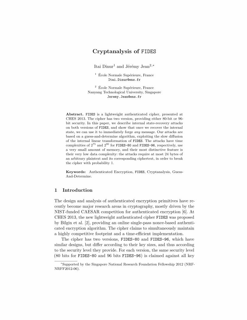
The full encryption/authentication process in visualized in Figure 2.We note that in order to decrypt, a similar process is performed, wherethe ciphertext is XORed with the leaked nibbles in order to decrypt and

3Since our attacks do not use any associated data, we do not elaborate on itsprocessing.

c bits

Figure 1: The 32c-bit internal state of FIDES, where X[3, 0] and X[3, 2] act as in-put/output during the encryption process.

obtain the message block, which is then XORed into the state. Finally,the tag is calculated and validated against the one received.

16R

ound

s

K||N

16c

K||0

2c

A0

1R

ound

2c

A1

1R

ound

• • •

1R

ound

2c

Av−1

1R

ound

C0 M0

2c

2c

1R

ound

• • •

1R

ound

Cn−1 Mn−1

2c

2c

16R

ound

s

Trun

cate

T

Figure 2: The encryption/authentication process of FIDES.

Description of the Round Function. The round function of FIDESuses AES-like transformations (see Figure 3).

At the beginning of round i, the two nibbles of the message block Mi

are processed and injected to produce the state Xi. The SubBytes (SB)transformation applies a non-linear S-Box S to each nibble of the stateXi independently, and the ShiftRows (SR) transformation rotates the r’throw by τ [r] positions to the left, where τ = [0, 1, 2, 7]. This produces astate that we denote by Yi. The state is then updated to the state Wi byapplying the linear transformation MixColumns (MC), which left-multiplieseach column of Yi independently by the binary matrix M:

M =

0 1 1 11 0 1 11 1 0 11 1 1 0

.

Finally, the AddConstant (AC) transformation XORs a 32-nibble round-dependent constant RCi (where RCi[`, j] denotes the nibble at position(`, j)) into the state Wi to produce the initial state of the next round,Xi+1. Since we assume that both the round constants and the messageblocks are known to us, we can obtain an equivalent scheme by removingthe message injections and “embedding” them to the round constants,XORed into the state at the end of the previous round. Thus, for the sakeof simplicity, we ignore the message injections in the rest of this paper.

We note that since our attack is structural, it is independent of theparticular choices of S-boxes and round-constants of FIDES. Thus, we omittheir description, which can be found in [2].4

Inj

Mi

SB

SR

Xi

MC

Yi

AC

Wi

RCi

Xi+1

Figure 3: The round function of FIDES.

3 Design Properties of FIDES Exploited in our Attacks

In this section, we emphasize the properties of FIDES that we exploit inour attacks. First, we describe two basic linear properties of the roundfunction that are extensively used in our state-recovery attack. Then,we describe two design properties of FIDES, and use them to show thatany state-recovery attack immediately enables the attacker to forge anymessage.

3.1 Properties of the MixColumns Transformation

The binary matrix M (that defines the MixColumns transformation) hasa branch number of 4. This implies that there are linear dependenciesbetween 4 nibbles of x and y = Mx (where x = [x0, x1, x2, x3] andy = [y0, y1, y2, y3]):

Property 1. For all i, j ∈ {0, 1, 2, 3} such that i 6= j: xi ⊕ xj = yi ⊕ yj .

Property 2. For all i ∈ {0, 1, 2, 3}: xi+3 = yi⊕xi+1⊕xi+2 (where additionis performed modulo 4), and (analogously): yi+3 = xi ⊕ yi+1 ⊕ yi+2.

Such equalities are extremely useful in guess-and-determine attackson AES-based schemes, where the attacker guesses a few internal nibblesof various states and tries to determine the values of as many nibbles aspossible in order to verify his guesses. Indeed, as the branch number ofM is 4, it is possible to determine the value of an unknown nibble of x ory, given the values of only 3 out of the 4 nibbles in an equation above.

4In fact, the round-constants are also not defined in the specifications.

We note that the maximal possible branch number for a 4× 4 matrixis 5 (the AES MixColumns transformation was especially designed to havethis property). Interestingly, the matrix M of FIDES was not be designedto have the maximal branch number due to implementation efficiencyconsiderations. As we demonstrate in our attack, this is a significantdesign-flaw. Indeed, we use the two properties above more than 150 timesin order to mount a state-recovery attack which is faster than exhaustivesearch.

3.2 Properties Exploited in Forgery Attacks

In this section, we show that a state-recovery attack enables the attackerto forge any message. This is a result of two design properties (refer toSection 2 for details):

Property 3. The initial internal state of FIDES is computed using a secretkey K and a public nonce N , and does not depend on the encryptedmessage.

Property 4. Once the internal state has been recovered, the rest of thecomputation (including the tag generation process) does not depend onK, and can be fully simulated for any message.

As a result of Property 3, once we recover the internal state generatedby one (K,N) pair in the encryption process of an arbitrary plaintext M ,we can immediately deduce it for the encryption of any other plaintextM ′, encrypted using the same (K,N) pair. Combined with Property 4, astate-recovery attack therefore enables to immediately forge any messageby simulating the encryption process and computing the produced tag.

We note that the design of FIDES places a restriction on the encryptiondevice, such that it cannot send two different messages with the same(K,N) pair. However, the ciphertexts decrypted by the decryption deviceare not restricted in such a way, namely, the device is allowed to decrypttwo ciphertexts with the same (K,N) pair (assuming that their tag isvalid). Thus, our attacks are applicable in the weak known plaintext model,and do not require advanced capabilities (such as intercepting messages,required in man-in-the-middle attacks).

4 Overview of the State-Recovery Attack

In this section, we give an overview of our state-recovery attack on bothversions of FIDES, distinguished by the nibble size of c bits. As any

meaningful attack must be more efficient than exhaustive search, we firstformalize the state-recovery problem for FIDES and analyze the simpleexhaustive search algorithm.

The State-Recovery Problem and Exhaustive Search. The inputto the state-recovery problem is a messageM , its corresponding ciphertextC, encrypted using a key/nonce pair (K,N), and the actual value of thenonce N .5 The goal of this problem is to recover X0, which denotes the32 nibbles of the initial state obtained after the initialization of FIDESwith the (K,N) pair. In order to recover the initial state, it is possible toexhaustively enumerate the 232c possibilities for X0 and check if each oneof them encrypts6 M to C. However, a much more efficient exhaustivesearch procedure is to enumerate all the 216c possibilities for the key. Sincethe nonce is known, one executes the initialization procedure of FIDESfor each value of the key, obtains a suggestion for X0, and then uses it toverify that M is indeed encrypted to C.

Complexity Evaluation of our Attack. As shown above, the timecomplexity of (efficient) exhaustive search for X0 is about 216c iterations(or time-units), where in each iteration, FIDES is initialized using 16round function evaluations (and additional few rounds in order to verifythat M is indeed encrypted to C). As described in the detailed attack(Section 5), compared to exhaustive search, the time complexity of ourstate-recovery attack is only 215c time-units. Moreover, in each such time-unit, we perform computations on c-bit nibbles that are equivalent to onlyabout nine FIDES round function evaluations (in addition to a few memorylook-ups). However, as this smaller time-unit does not give our attack anadditional significant advantage over exhaustive search, we ignore it inthe remainder of this paper, and assume for the sake of simplicity thatour attack uses the exhaustive search time-unit.

In terms of memory, the basic unit that we use contains 32 nibbles,which is the size of the FIDES internal state.

4.1 The Main Procedure of our Attack

The attack uses the knowledge of a single 9-block known-plaintext mes-sage M0|| · · · ||M8, and we denote by C0|| · · · ||C8 the associated ciphertext.

5One may also include the tag of the message in the inputs to the state-recoveryproblem, however, we do not require it.

6Recall that after the initialization, the encryption process does not depend on K,and thus X0 fully determines the result of the encryption.

Algorithm 1 – Main Procedure of the State-Recovery Attack.1: function StateRecovery2: Guess nibbles of N1 # Step 1 – |N1| =12 nibbles3: Determine values for nibbles of N ′1 # Step 14: Construct table T1 # Step 2a – 23c operations5: Construct table T2 # Step 2b – 23c operations6: Guess nibbles of N2 # Step 3a – |N2| =3 nibbles7: Determine values for nibbles of N ′2 # Step 3a8: Use table T1 to determine additional nibbles # Step 3b9: Use table T2 to determine internal state # Step 3c10: if all output nibbles are consistent then # p = 2−c

11: return State # 212c+3c−c = 214c states

Thus, according to the design of FIDES (see Section 2), we have the knowl-edge of two nibbles of c bits in 9 consecutive internal states X0, . . . , X8,linked by 8 rounds. The attack enumerates in 215c computations the ex-pected number of 2(32−2×9)×c = 214c valid states (i.e., solutions) whichcan possibly produce C0|| · · · ||C8. By using additional output (given byadditional ciphertext blocks, or by the tag corresponding to the message),we can post-filter these states and recover the correct internal state X0(which allows us to determine all Xi for i ≥ 0) with a time complexityof 215c computations. This is less than the time complexity of exhaustivesearch by a factor of 2c.

The main procedure of the attack is given in Algorithm 1, where thenibble sets N1, N ′1, N2 and N ′2 are defined in Section 5.

The first step (Step 1 – lines 2,3) consists of an initial guess-and-determine phase. The following two steps (Step 2a – line 4 and Step 2b– line 5) construct the look-up tables T1 and T2, respectively. These twosteps are independent of each other, however, both of them depend onStep 1. In the final steps of the attack, we perform an additional guess-and-determine phase (Step 3a – lines 6,7), use the look-up table T1 inorder to determine the values of additional nibbles (Step 3b – line 8), anduse the look-up table T2 in order to determine the full state (Step 3c –line 9). Finally, we post-filter the remaining states (line 10) to return the214c valid states. We note that these states are returned and post-filtered“on-the-fly”, and thus the memory complexity of the attack is only 23c

(which is the size of the look-up tables T1 and T2).

4.2 The Structure of the Steps in our Attack

In general, all the steps of the attack are comprised of guessing/enumeratingthe values of several nibbles of the internal states X0, . . . , X8, and thenpropagating the knowledge forwards and backwards through the states.The knowledge propagation uses a small number of simple equalities E(formally defined in Section 4) that are derived from the internal mappingsof FIDES.

As X0, . . . , X8 contain hundreds of nibbles, our attack uses hundreds ofcomputations on the nibbles in order to propagate the knowledge throughthe states. As a result, manual verification of the attack is rather tedious.On the other hand, it is important to stress that automatic verification ofthe attack is rather simple, as one needs to program the main procedureof Algorithm 1 with the nibbles that are guessed/enumerated in each step.The program greedily propagates the knowledge through the states usingE, until X0 is recovered.

Despite the simplicity of the automatic verification, we still aim to givethe reader a good intuition of how the knowledge is propagated throughoutthe attack without listing all of its calculations in the text (which wouldmake the paper very difficult to read). Thus, we provide in the next sectionfigures that visualize the determined nibbles of the state after each step,and for the sake of completeness, we additionally provide in Section Ctables that describe some of the low-level calculations.

The Look-up Tables T1 and T2. We conclude this section with aremark regarding the look-up tables T1 and T2: as each one of these look-up tables is constructed using simple equalities, it may raise the concernthat they do not contribute to the attack. Namely, it may seem possible tosimply guess the 15 nibbles of N1 and N2 in the outer loop of the attackand recover the internal state by propagating the knowledge using simpleequations. However, the data that the look-up tables store is inverted andindexed in a way which cannot be described using simple equations. In fact,the look-up tables are used in meet-in-the-middle algorithms (Steps 3band 3c) in order to propagate the information in a more complex way.

5 Details of the State-Recovery Attack

In this section, we describe in detail all the steps of the attack. For eachstep, we use a figure that visualizes the nibbles of the state that we guessor enumerate, and the nibbles that we determine using E. For the sake of

completeness, we additionally provide in Section C tables that describehow we use the equalities of E in each step.

We partition E into two groups, E1 and E2, where E = E1⋃E2.

The first group E1 contains equalities that are directly derived fromthe FIDES internal mappings AddConstant,SubBytes,ShiftRows (appliedindependently to each nibble) and MixColumns (applied independently toeach column), in addition to their inverses. The equalities of E1 can onlybe directly applied to a single nibble or a column of the state. The secondgroup E2 contains the linear equalities of Section 3.1. These equalities aresomewhat less “trivial” as they can be used in several ways in order tofactor out an unknown variable (or a linear combination of variables), andexpress it as a linear combination of variables from one column of a stateor two columns of two states, linked by MixColumns.

In order to avoid very big tables, Section C lists only the equalitiesof E2 in a potential ordering7 in which these equalities can be applied inorder to derive the values of the internal state variables Xi (for 0 ≤ i ≤ 8).A reader interested in manually propagating the knowledge according tothe figures, may use these tables in combination with the E1 equalities, inorder to propagate the knowledge of the nibbles of Xi forwards to Yi, andbackwards to Wi−1.

5.1 Step 1: Initial Guess-and-Determine

We start by guessing the values of the following 12 nibbles that define theset N1 (see hatched nibbles in Figure 4):

N1def=

X3[0, 0], X3[0, 1], X3[0, 2], X3[3, 1],X4[1, 0], X4[1, 1], X4[1, 2],X5[0, 0], X5[0, 1], X5[0, 2],X6[0, 0], X6[3, 1]

.

Then, we propagate their values throughout the state. All the nibblesdetermined at the end of this step define the nibble-set N ′1, and are givenin Figure 4. The nibbles determined using the properties of the M matrixare given in Table 3.

We note that Step 1 depends on the known leaked nibbles Xi[3, 0] andXi[3, 2] for 1 ≤ i ≤ 7. However, this step is independent of the values ofX0[3, 0], X0[3, 2], X8[3, 0] and X8[3, 2].

7There exist different orderings leading to the same result.

SB

SR

X0

MC

Y0 W0

#0

SB

SR

X1

MC

Y1 W1

#1

SB

SR

X2

MC

Y2 W2

#2

SB

SR

X3

MC

Y3 W3

#3

SB

SR

X4

MC

Y4 W4

#4

SB

SR

X5

MC

Y5 W5

#5

SB

SR

X6

MC

Y6 W6

#6

SB

SR

X7

MC

Y7 W7

#7

SB

SR

X8

MC

Y8 W8

#8

Legend

Unknown valueKnown valueGuessed value (N1)Determined value (N ′

1)

Figure 4: Step 1: Initial guess-and-determine.

In total, given the 18 leaked nibbles, we expect about 2(32−18)c = 214c

conforming internal states, and thus after we guess the values of 12nibbles, we expect to reduce the number of solutions to 2(14−12)c = 22c.In the sequel, we describe how to enumerate these 22c solutions in 23c

computations and 23c memory.

5.2 Step 2a: Construction of T1

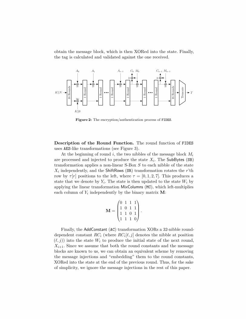
In this step, we use the values of the nibbles of N1 ∪ N ′1 to constructthe look-up table T1, which contains 23c entries. During its construction,we enumerate all the possible values of the 3 nibbles X1[2, 1], X2[2, 0]and X2[1, 7], and for each such value, we calculate and store the valuesdescribed in Figure 5. As an index to the table, we choose the following

triplet of independent linear relations of the computed nibbles

(W1[1, 7]⊕ Y1[2, 7], Y1[1, 0]⊕W1[2, 0], Y2[1, 6]⊕ Y2[2, 6]

).

SB

SR

X0

MC

Y0 W0

#0

SB

SR

X1

MCNH

Y1 W1

NH#1

SB

SR

X2

MC••

Y2 W2

#2

Legend

Unknown valueKnown valueEnumerated valueDetermined value

•NH

Index for T1

Figure 5: Step 2a: construction of T1.

As this step is relatively short, we describe it in Section B. Additionally,we provide in Table 4 the list of nibbles determined using the propertiesof the M matrix. We note that unlike Step 1, this step depends on thevalue of the known nibble X0[3, 0].

5.3 Step 2b: Construction of T2

In this step, we use the values of the nibbles of N1 ∪ N ′1 to constructthe second look-up table T2, which (similarly to T1) contains 23c entries.During its construction, we enumerate all the possible values of the 3nibbles X4[1, 6], X5[1, 4] and X6[2, 4], and for each such value, we calculateand store the values described in Figure 6. As an index to the table, wechoose the following triplet of nibbles/linear relations of the computednibbles

(W3[1, 6]⊕W3[2, 6], Y4[2, 5], Y7[1, 0]⊕ Y7[2, 0]

).

The nibbles that are determined using the properties of the matrix Mare described in Table 5 (which also describes a possible ordering of thecomputations). We note that this step depends on the value of X8[3, 0](unlike Step 1 and Step 2a).

SB

SR

X0

MC

Y0 W0

#0

SB

SR

X1

MC

Y1 W1

#1

SB

SR

X2

MC

Y2 W2

#2

SB

SR

X3

MC

Y3 W3

••#3

SB

SR

X4

MCNY4 W4

#4

SB

SR

X5

MC

Y5 W5

#5

SB

SR

X6

MC

Y6 W6

#6

SB

SR

X7

MCHH

Y7 W7

#7

SB

SR

X8

MC

Y8 W8

#8

Legend

Unknown valueKnown valueEnumerated valueDetermined value

•NH

Index for T2

Figure 6: Step 2b: construction of T2.

5.4 Step 3a: Final Guess-and-DetermineIn this step, we guess 3 additional nibbles to the 12 initial ones (seehatched nibbles on Figure 7):

N2def={X1[0, 3], X1[1, 3], X3[2, 7]

}.

Their values allow to determine all the values marked in gray onFigure 7, which define the set N ′2. We list all the nibbles of N ′2, determinedusing the properties of the M matrix in Table 6. We note that unlike theprevious steps, this step depends on the value of the leaked nibble X0[3, 2].

5.5 Step 3b: Table T1 Look-UpIn this step, we perform a look-up in table T1 in order to determine thevalues of additional nibbles, and then propagate the knowledge further

SB

SR

X0

MC

Y0 W0

#0

SB

SR

X1

MC

Y1 W1

#1

SB

SR

X2

MC

Y2 W2

#2

SB

SR

X3

MC

Y3 W3

#3

SB

SR

X4

MC

Y4 W4

#4

SB

SR

X5

MC

Y5 W5

#5

SB

SR

X6

MC

Y6 W6

#6

SB

SR

X7

MC

Y7 W7

#7

SB

SR

X8

MC

Y8 W8

#8

Legend

Unknown valueKnown valueGuessed value (N2)Determined value (N ′

2)

Figure 7: Step 3a: three more nibbles are guessed to determine more values.

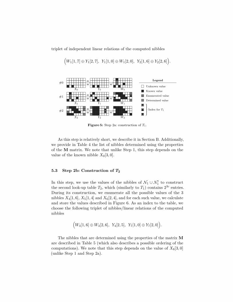
through the internal state. We access T1 using the determined values ofW1[0, 7]⊕W1[3, 7], W1[1, 0]⊕ Y1[2, 0] and W2[1, 6]⊕W2[2, 6] (see nibblesN, H and • in Figure 8). Indeed, using the properties of the matrix M:

W1[0, 7]⊕W1[3, 7] = Y1[2, 7]⊕W1[1, 7]W1[1, 0]⊕ Y1[2, 0] = Y1[1, 0]⊕W1[2, 0]W2[1, 6]⊕W2[2, 6] = Y2[1, 6]⊕ Y2[2, 6],

where the right-hand sides define the elements of the index triplet to thetable T1. As T1 contains 23c entries, we expect one match on averagefor each table look-up, which immediately determines all the additionalhatched values in Figure 8.

SB

SR

X0

MC

Y0 W0

#0

SB

SR

X1

MCHY1 W1

#1N

NH

SB

SR

X2

MC

Y2 W2

#2 ••

SB

SR

X3

MC

Y3 W3

#3

SB

SR

X4

MC

Y4 W4

#4

SB

SR

X5

MC

Y5 W5

#5

SB

SR

X6

MC

Y6 W6

#6

SB

SR

X7

MC

Y7 W7

#7

SB

SR

X8

MC

Y8 W8

#8

Legend

Unknown valueKnown valueLooked-up value in T1

Determined value•NH

Look-up index for T1

Figure 8: Step 3b: table T1 look-up.

After the table T1 look-up, we propagate the additional knowledgethrough the internal states. We list in Table 7 the additional nibbles thatwe can determine using the properties of the matrix M.

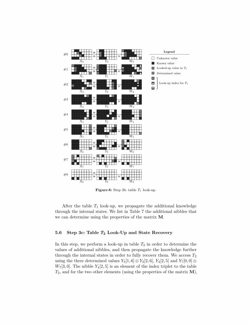
5.6 Step 3c: Table T2 Look-Up and State Recovery

In this step, we perform a look-up in table T2 in order to determine thevalues of additional nibbles, and then propagate the knowledge furtherthrough the internal states in order to fully recover them. We access T2using the three determined values Y3[1, 6]⊕ Y3[2, 6], Y4[2, 5] and Y7[0, 0]⊕W7[3, 0]. The nibble Y4[2, 5] is an element of the index triplet to the tableT2, and for the two other elements (using the properties of the matrix M),

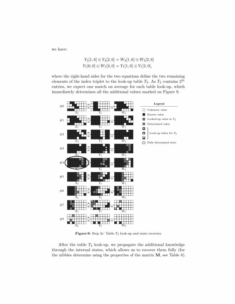
we have:

Y3[1, 6]⊕ Y3[2, 6] = W3[1, 6]⊕W3[2, 6]Y7[0, 0]⊕W7[3, 0] = Y7[1, 0]⊕ Y7[2, 0],

where the right-hand sides for the two equations define the two remainingelements of the index triplet to the look-up table T2. As T2 contains 23c

entries, we expect one match on average for each table look-up, whichimmediately determines all the additional values marked on Figure 9.

SB

SR

X0

MC

Y0 W0

#0

SB

SR

X1

MC

Y1 W1

#1

SB

SR

X2

MC

Y2 W2

#2

SB

SR

X3

MC••

Y3 W3

#3

SB

SR

X4

MCNY4 W4

#4

SB

SR

X5

MC

Y5 W5

#5

SB

SR

X6

MC

Y6 W6

#6

SB

SR

X7

MC

H

Y7 W7

#7H

SB

SR

X8

MC

Y8 W8

#8

Legend

Unknown valueKnown valueLooked-up value in T2

Determined value•NH

Look-up index for T2

Fully determined state

Figure 9: Step 3c: Table T2 look-up and state recovery

After the table T2 look-up, we propagate the additional knowledgethrough the internal states, which allows us to recover them fully (forthe nibbles determine using the properties of the matrix M, see Table 8).

Namely, we fully recover X4 by the following operations:

W3[0, 6] = Y3[1, 6]⊕W3[2, 6]⊕W3[3, 6]X4[0, 6] = W3[0, 6]⊕RC3[0, 6]Y4[0, 5] = W4[1, 5]⊕ Y4[2, 5]⊕ Y4[3, 5]X4[0, 5] = S−1(Y4[0, 5])W3[3, 5] = W3[0, 5]⊕W3[1, 5]⊕ Y3[2, 5]X4[3, 5] = W3[3, 5]⊕RC3[3, 5].

Given X4, we can compute all the states forwards and backwards.

Post-Filtering. Once the internal state is fully determined, we verifythat the additional output X8[3, 2] matches its leaked value. Indeed, the18 leaked nibbles have all been used in the attack, with the exception ofthe very last one, X8[3, 2]. As this match occurs with probability 2−c, thealgorithm indeed enumerates the 214c internal states that produce the 18leaked nibbles in about 2(12+3)c = 215c computations, using a memory ofabout 23c elements. Finally, we can post-filter the solutions further usingadditional output (given by additional ciphertext blocks, or by the tagcorresponding to the message).

6 Conclusions and Open Problems

In this paper, we presented state-recovery attacks on both versions ofFIDES, and showed how to use them in order to forge messages. Ourattacks use a guess-and-determine algorithm in order to break the securityof the primitive given very little data and a small amount of memory.

A simple way to repair FIDES such that it would resist our attacks, isto use a linear transformation with a branch number of 5. However, thiswould have a negative impact on the efficiency of the implementation, andmoreover, it is unclear whether such a change would guarantee resistanceagainst different (perhaps more complex) guess-and-determine attacks. Ingeneral, although the leak-extraction notion allows building cryptosystemswith very efficient implementations, designing such systems which alsooffer a large security margin remains a challenging task for the future. Inparticular, it would be very interesting to design such cryptosystems whichprovably resist guess-and-determine attacks, such as the ones presented inthis paper.

References

1. Bertoni, G., Daemen, J., Peeters, M., Assche, G.V.: Duplexing the Sponge: Single-Pass Authenticated Encryption and Other Applications. In Miri, A., Vaudenay, S.,eds.: Selected Areas in Cryptography. Volume 7118 of Lecture Notes in ComputerScience., Springer (2011) 320–337

2. Bilgin, B., Bogdanov, A., Knezevic, M., Mendel, F., Wang, Q.: FIDES: LightweightAuthenticated Cipher with Side-Channel Resistance for Constrained Hardware.In Bertoni, G., Coron, J.S., eds.: CHES 2013. Volume 8086 of LNCS., Springer(August 2013) 142–158

3. Biryukov, A.: The Design of a Stream Cipher LEX. In Biham, E., Youssef, A.M.,eds.: SAC 2006. Volume 4356 of LNCS., Springer (August 2006) 67–75

4. Bogdanov, A., Mendel, F., Regazzoni, F., Rijmen, V., Tischhauser, E.: ALE: AES-Based Lightweight Authenticated Encryption. In: FSE. Lecture Notes in ComputerScience (2013) to appear.

5. Bouillaguet, C., Derbez, P., Fouque, P.A.: Automatic Search of Attacks on Round-Reduced AES and Applications. In Rogaway, P., ed.: CRYPTO 2011. Volume 6841of LNCS., Springer (August 2011) 169–187

6. CAESAR: Competition for Authenticated Encryption: Security, Applicability, andRobustness. http://competitions.cr.yp.to/caesar.html.

7. Daemen, J., Rijmen, V.: The Design of Rijndael: AES - The Advanced EncryptionStandard. Springer (2002)

8. Dunkelman, O., Keller, N.: A New Attack on the LEX Stream Cipher. In Pieprzyk,J., ed.: ASIACRYPT 2008. Volume 5350 of LNCS., Springer (December 2008)539–556

9. Khovratovich, D., Rechberger, C.: The LOCAL attack: Cryptanalysis of theauthenticated encryption scheme ALE. In: SAC. Lecture Notes in Computer Science(2013) to appear.

10. Suzuki, K., Tonien, D., Kurosawa, K., Toyota, K.: Birthday Paradox for Multi-collisions. In Rhee, M.S., Lee, B., eds.: ICISC 06. Volume 4296 of LNCS., Springer(November / December 2006) 29–40

11. Wu, S., Wu, H., Huang, T., Wang, M., Wu, W.: Leaked-State-Forgery Attackagainst the Authenticated Encryption Algorithm ALE. In Sako, K., Sarkar, P., eds.:ASIACRYPT (1). Volume 8269 of Lecture Notes in Computer Science., Springer(2013) 377–404

A Exploiting More Data to Optimize the Attack

The basic state-recovery attack of Section 4 requires only a single messageof at most 24 bytes in order to recover the state faster than exhaustivesearch. This is a devastating attack, as once the state is recovered, itenables the attacker to immediately forge messages. In this section, weshow that given more data, we can forge messages even faster by recoveringan internal state (obtained during the encryption process of one of thesemessages) more efficiently.

In order to describe the optimization, we first recall that the basicattack is composed of two phases: in the first phase, the attack requires 17c

bits of leakage (computed using the ciphertext) in order to enumerate in215c time the expected number of 2(32−17)c = 215c internal states (solutions)that can possibly produce the leaked bits. In the second phase of the attack,these solutions are post-filtered8 according to additional given ciphertextblocks (or the produced tag).

Our optimization can be applied if we obtain t ≥ 2 messages for whichthe 17c leaked bits have the same (arbitrary) value. Namely, we obtain at-way collision on Xi[3, 0] for 0 ≤ i ≤ 8 and Xj [3, 2] for 0 ≤ j ≤ 7. Then,we can run the first phase of the algorithm using this particular value. Inthis case, each solution produced and post-filtered “on-the-fly” is t timesmore likely to match one of the t internal states corresponding to the tmessages. Consequently, we expect the algorithm to recover a first internalstate among these t possibilities in a reduced time of 215c/t.

According to standard randomness assumptions, the leaked bits ofthe messages we obtain are distributed uniformly and independently.Hence, in order to obtain a t-way collision on 17c leaked bits, we requireabout 217c(t−1)/t messages.9 In particular, for FIDES-80 we expect a 4-way collision on the 17 · 5 = 85 output bits, required in the first phase ofthe attack, after obtaining about 217·5·(4−1)/4 ≈ 264 messages. Thus, wecan forge messages in an expected time complexity of 215·5 · 1/4 = 273

computations. For FIDES-96, we expect a 4-way collision on the required17 · 6 = 102 output bits given 217·6·(4−1)/4 ≈ 277 messages, enabling us toforge messages in time complexity of 217·6 · 1/4 = 288 computations.

The following Table 2 lists the additional tradeoff points between dataand time.

Table 2: Tradeoff points between data and time.FIDES-80 (c = 5) FIDES-96 (c = 6)

t Data (KP) Time Data (KP) Time2 242.50 274.00 251.00 289.00

3 256.67 273.42 268.00 288.42

4 263.75 273.00 276.50 288.00

5 268.00 272.68 281.60 287.68

6 270.83 272.42 285.00 287.42

KP: known plaintext

8We remind the reader that the solutions are post-filtered “on-the-fly”, rather thanstored in memory.

9In order to obtain a t-way collision on the n-bit output of a random map, oneneeds to evaluate it (t!)1/t · 2n(t−1)/t times [10], which is approximately 2n(t−1)/t whent is small.

B Details of Step 2a

We fully describe Step 2a in the text below.

1. For each value of X1[2, 1]:(a) Compute W0[2, 1] = X1[2, 1]⊕RC0[2, 1].(b) Compute W0[1, 1]: using property 2 of the matrix M, we have

Y0[3, 1] = W0[0, 1] ⊕ W0[1, 1] ⊕ W0[2, 1], and thus W0[1, 1] =Y0[3, 1] ⊕ W0[0, 1] ⊕ W0[2, 1]. Note that W0[0, 1] has been com-puted in Step 1, and Y0[3, 1] = S(X0[3, 0]) is a leaked value.

(c) Compute X1[1, 1] = W0[1, 1]⊕RC0[1, 1].(d) Compute Y1[1, 0] = S(X1[1, 1]).(e) Compute Y1[2, 7] = S(X1[2, 1]).(f) For each value of X2[2, 0]:

i. Compute Y2[2, 6] = S(X2[2, 0]).ii. Compute W1[2, 0] = X2[2, 0]⊕RC1[2, 0].iii. ComputeW1[0, 0] = Y1[1, 0]⊕W1[2, 0]⊕W1[3, 0] (using property

2 of M).iv. Compute X2[0, 0] = W1[0, 0]⊕RC1[0, 0].v. Compute Y2[0, 0] = S(X2[0, 0]).vi. Compute Y2[3, 0]: using property 1 of the M, we have Y2[0, 0]⊕

Y2[3, 0] = W2[0, 0] ⊕W2[3, 0], and thus Y2[3, 0] = W2[0, 0] ⊕W2[3, 0]⊕Y2[0, 0]. Note thatW2[0, 0] is known from Step 1, andW2[3, 0] = X3[3, 0]⊕RC2[3, 0] is a leaked value.

vii. Compute X2[3, 7] = S−1(Y2[3, 0]).viii. Compute W1[3, 7] = X2[3, 7]⊕RC1[3, 7].ix. For each value of X2[1, 7]:

A. Compute Y2[1, 6] = S(X2[1, 7]).B. Compute W1[1, 7] = X2[1, 7]⊕RC1[1, 7].C. ComputeW1[0, 7]: using property 2 of M, we haveW1[0, 7] =

Y1[2, 7]⊕W1[1, 7]⊕W1[3, 7]. Note that Y1[2, 7], W1[1, 7] andW1[3, 7] are all determined at this stage.

D. Compute X2[0, 7] = W1[0, 7]⊕RC1[0, 7].E. Compute Y2[0, 7] = S(X2[0, 7]).F. Allocate an entry in T1 with the index triplet (W1[1, 7]⊕

Y1[2, 7], Y1[1, 0]⊕W1[2, 0], Y2[1, 6]⊕ Y2[2, 6]), and store thevalues of all the nibbles computed above.

C Tables for the State-Recovery Attack

In this appendix, we give tables which describe how we propagate theknowledge in the state-recovery attack using the properties of the M

matrix (described in Section 3.1), and a potential ordering in which theycan be used.

Table 3: Nibbles determined in Step 1 using the properties of the M matrix# Pr. Nibble Equation # Pr. Nibble Equation1 2 X4[2, 0] RC4[2, 0]⊕Y3[0, 0]⊕W3[1, 0]⊕W3[3, 0] 34 2 X5[2, 1] RC5[2, 1]⊕ Y4[0, 1]⊕ Y4[1, 1]⊕ Y4[3, 1]2 2 X4[2, 2] RC4[2, 2]⊕Y3[0, 2]⊕W3[1, 2]⊕W3[3, 2] 35 1 X5[3, 1] RC5[3, 1]⊕Y4[3, 1]⊕Y4[0, 1]⊕W4[0, 1]3 1 X3[2, 4] S−1(Y3[3, 2]⊕W3[2, 2]⊕W3[3, 2]) 36 2 X4[2, 3] S−1(W4[0, 1]⊕W4[1, 1]⊕W4[3, 1])4 1 X3[1, 3] S−1(Y3[2, 2]⊕W3[1, 2]⊕W3[2, 2]) 37 1 X5[3, 7] S−1(Y5[0, 0]⊕W5[3, 0]⊕W5[0, 0])5 2 X4[0, 2] RC4[0, 2]⊕ Y3[1, 2]⊕ Y3[2, 2]⊕ Y3[3, 2] 38 1 X6[0, 1] RC6[0, 1]⊕Y5[0, 1]⊕Y5[3, 1]⊕W5[3, 1]6 1 X4[3, 1] S−1(Y4[0, 2]⊕W4[3, 2]⊕W4[0, 2]) 39 1 X6[1, 0] RC6[1, 0]⊕Y5[1, 0]⊕Y5[0, 0]⊕W5[0, 0]7 1 X3[1, 2] S−1(Y3[3, 1]⊕W3[1, 1]⊕W3[3, 1]) 40 2 X5[2, 2] S−1(W5[0, 0]⊕W5[1, 0]⊕W5[3, 0])8 2 X4[2, 1] RC4[2, 1]⊕ Y3[0, 1]⊕ Y3[1, 1]⊕ Y3[3, 1] 41 2 X6[2, 0] RC6[2, 0]⊕ Y5[0, 0]⊕ Y5[1, 0]⊕ Y5[3, 0]9 1 X3[2, 3] S−1(Y3[1, 1]⊕W3[2, 1]⊕W3[1, 1]) 42 1 X6[0, 2] RC6[0, 2]⊕Y5[0, 2]⊕Y5[3, 2]⊕W5[3, 2]10 2 X4[0, 1] RC4[0, 1]⊕ Y3[1, 1]⊕ Y3[2, 1]⊕ Y3[3, 1] 43 1 X7[0, 2] RC7[0, 2]⊕Y6[0, 2]⊕Y6[3, 2]⊕W6[3, 2]11 2 X5[2, 0] RC5[2, 0]⊕Y4[1, 0]⊕W4[0, 0]⊕W4[3, 0] 44 2 X4[1, 3] RC4[1, 3]⊕Y3[0, 3]⊕Y3[3, 3]⊕W3[2, 3]12 1 X5[1, 0] RC5[1, 0]⊕Y4[1, 0]⊕Y4[2, 0]⊕W4[2, 0] 45 1 X4[2, 4] S−1(Y4[0, 2]⊕W4[2, 2]⊕W4[0, 2])13 2 X4[0, 0] S−1(W4[1, 0]⊕W4[2, 0]⊕W4[3, 0]) 46 2 X5[1, 2] RC5[1, 2]⊕ Y4[0, 2]⊕ Y4[2, 2]⊕ Y4[3, 2]14 2 X4[3, 7] S−1(W4[0, 0]⊕W4[1, 0]⊕W4[2, 0]) 47 1 X6[1, 1] RC6[1, 1]⊕Y5[1, 1]⊕Y5[0, 1]⊕W5[0, 1]15 2 X3[1, 1] S−1(W3[0, 0]⊕W3[2, 0]⊕W3[3, 0]) 48 2 X6[2, 1] RC6[2, 1]⊕ Y5[0, 1]⊕ Y5[1, 1]⊕ Y5[3, 1]16 2 X3[2, 2] S−1(W3[0, 0]⊕W3[1, 0]⊕W3[3, 0]) 49 2 X5[2, 3] S−1(W5[0, 1]⊕W5[1, 1]⊕W5[3, 1])17 2 X3[3, 7] S−1(W3[0, 0]⊕W3[1, 0]⊕W3[2, 0]) 50 2 X6[2, 2] S−1(Y6[0, 0]⊕ Y6[1, 0]⊕W6[3, 0])18 1 X2[0, 1] S−1(Y2[3, 1]⊕W2[0, 1]⊕W2[3, 1]) 51 1 X5[2, 4] S−1(Y5[0, 2]⊕W5[2, 2]⊕W5[0, 2])19 1 X2[1, 2] S−1(Y2[0, 1]⊕W2[1, 1]⊕W2[0, 1]) 52 2 X5[1, 3] S−1(W5[0, 2]⊕W5[2, 2]⊕W5[3, 2])20 2 X2[2, 3] S−1(W2[0, 1]⊕W2[1, 1]⊕W2[3, 1]) 53 2 X6[1, 2] RC6[1, 2]⊕ Y5[0, 2]⊕ Y5[2, 2]⊕ Y5[3, 2]21 2 X3[2, 1] RC3[2, 1]⊕ Y2[0, 1]⊕ Y2[1, 1]⊕ Y2[3, 1] 54 2 X7[2, 1] RC7[2, 1]⊕ Y6[0, 1]⊕ Y6[1, 1]⊕ Y6[3, 1]22 2 X2[0, 2] S−1(W2[1, 2]⊕W2[2, 2]⊕W2[3, 2]) 55 2 X5[0, 3] RC5[0, 3]⊕Y4[3, 3]⊕W4[1, 3]⊕W4[2, 3]23 2 X2[1, 3] S−1(W2[0, 2]⊕W2[2, 2]⊕W2[3, 2]) 56 2 X3[2, 5] S−1(Y3[0, 3]⊕ Y3[3, 3]⊕W3[1, 3])24 2 X2[2, 4] S−1(W2[0, 2]⊕W2[1, 2]⊕W2[3, 2]) 57 1 X3[1, 4] S−1(Y3[2, 3]⊕W3[1, 3]⊕W3[2, 3])25 2 X2[3, 1] S−1(W2[0, 2]⊕W2[1, 2]⊕W2[2, 2]) 58 2 X4[0, 3] RC4[0, 3]⊕ Y3[1, 3]⊕ Y3[2, 3]⊕ Y3[3, 3]26 2 X3[0, 3] RC3[0, 3]⊕Y2[3, 3]⊕W2[1, 3]⊕W2[2, 3] 59 2 X4[3, 3] RC4[3, 3]⊕ Y3[0, 3]⊕ Y3[1, 3]⊕ Y3[2, 3]27 1 X1[0, 1] S−1(Y1[3, 1]⊕W1[0, 1]⊕W1[3, 1]) 60 1 X4[1, 4] S−1(Y4[0, 3]⊕W4[1, 3]⊕W4[0, 3])28 2 X1[2, 4] S−1(W1[0, 2]⊕W1[1, 2]⊕W1[3, 2]) 61 1 X4[2, 5] S−1(Y4[0, 3]⊕W4[2, 3]⊕W4[0, 3])29 2 X2[0, 3] RC2[0, 3]⊕Y1[3, 3]⊕W1[1, 3]⊕W1[2, 3] 62 2 X5[3, 3] RC5[3, 3]⊕ Y4[0, 3]⊕ Y4[1, 3]⊕ Y4[2, 3]30 1 X3[3, 3] RC3[3, 3]⊕Y2[3, 3]⊕Y2[0, 3]⊕W2[0, 3] 63 2 X4[0, 4] RC4[0, 4]⊕Y3[3, 4]⊕W3[1, 4]⊕W3[2, 4]31 2 X2[1, 4] S−1(W2[0, 3]⊕W2[2, 3]⊕W2[3, 3]) 64 2 X4[1, 5] S−1(Y4[0, 4]⊕ Y4[3, 4]⊕W4[2, 4])32 2 X2[2, 5] S−1(W2[0, 3]⊕W2[1, 3]⊕W2[3, 3]) 65 2 X4[0, 7] S−1(Y4[1, 7]⊕ Y4[2, 7]⊕W4[3, 7])33 1 X5[1, 1] RC5[1, 1]⊕Y4[1, 1]⊕Y4[0, 1]⊕W4[0, 1] 66 2 X4[1, 7] RC4[1, 7]⊕Y3[2, 7]⊕W3[0, 7]⊕W3[3, 7]

Table 4: Nibbles determined in Step 2a using the properties of the M matrix# Property Nibble Equation1 2 X1[1, 1] RC1[1, 1]⊕ Y0[3, 1]⊕W0[0, 1]⊕W0[2, 1]2 2 X2[0, 0] RC2[0, 0]⊕ Y1[1, 0]⊕W1[2, 0]⊕W1[3, 0]3 1 X2[3, 7] S−1(Y2[0, 0]⊕W2[3, 0]⊕W2[0, 0])4 2 X2[1, 7] RC2[0, 7]⊕ Y1[2, 7]⊕W1[1, 7]⊕W1[3, 7]

Table 5: Nibbles determined in Step 2b using the properties of the M matrix# Pr. Nibble Equation # Pr. Nibble Equation1 1 X4[2, 6] S−1(Y4[1, 4]⊕W4[2, 4]⊕W4[1, 4]) 18 2 X5[2, 7] RC5[2, 7]⊕ Y4[0, 7]⊕ Y4[1, 7]⊕ Y4[3, 7]2 2 X5[0, 4] RC5[0, 4]⊕ Y4[1, 4]⊕ Y4[2, 4]⊕ Y4[3, 4] 19 1 X5[2, 5] S−1(Y5[1, 3]⊕W5[2, 3]⊕W5[1, 3])3 2 X5[3, 4] RC5[3, 4]⊕ Y4[0, 4]⊕ Y4[1, 4]⊕ Y4[2, 4] 20 1 X4[2, 7] S−1(Y4[1, 5]⊕W4[2, 5]⊕W4[1, 5])4 2 X6[2, 3] RC6[2, 3]⊕ Y5[0, 3]⊕ Y5[1, 3]⊕ Y5[3, 3] 21 2 X3[0, 7] S−1(W3[1, 7]⊕W3[2, 7]⊕W3[3, 7])5 2 X5[1, 5] S−1(Y5[0, 4]⊕ Y5[3, 4]⊕W5[2, 4]) 22 2 X3[1, 0] S−1(W3[0, 7]⊕W3[2, 7]⊕W3[3, 7])6 2 X7[0, 1] RC7[0, 1]⊕ Y6[1, 1]⊕ Y6[2, 1]⊕ Y6[3, 1] 23 2 X3[3, 6] S−1(W3[0, 7]⊕W3[1, 7]⊕W3[2, 7])7 2 X7[1, 1] RC7[1, 1]⊕ Y6[0, 1]⊕ Y6[2, 1]⊕ Y6[3, 1] 24 2 X3[0, 6] S−1(W3[1, 6]⊕W3[2, 6]⊕W3[3, 6])8 2 X7[3, 1] RC7[3, 1]⊕ Y6[0, 1]⊕ Y6[1, 1]⊕ Y6[2, 1] 25 2 X2[2, 2] S−1(W2[0, 0]⊕W2[1, 0]⊕W2[3, 0])9 1 X8[0, 2] RC8[0, 2]⊕ Y7[0, 2]⊕ Y7[3, 2]⊕W7[3, 2] 26 2 X1[0, 2] S−1(W1[1, 2]⊕W1[2, 2]⊕W1[3, 2])10 2 X7[1, 2] RC7[1, 2]⊕ Y6[0, 2]⊕ Y6[2, 2]⊕ Y6[3, 2] 27 2 X1[1, 3] S−1(W1[0, 2]⊕W1[2, 2]⊕W1[3, 2])11 1 X7[2, 2] RC7[2, 2]⊕ Y6[2, 2]⊕ Y6[0, 2]⊕W6[0, 2] 28 2 X1[3, 1] S−1(W1[0, 2]⊕W1[1, 2]⊕W1[2, 2])12 2 X6[1, 3] RC6[1, 3]⊕ Y5[0, 3]⊕ Y5[3, 3]⊕W5[2, 3] 29 1 X0[0, 1] S−1(Y0[3, 1]⊕W0[0, 1]⊕W0[3, 1])13 2 X7[0, 0] RC7[0, 0]⊕ Y6[1, 0]⊕ Y6[2, 0]⊕W6[3, 0] 30 2 X6[0, 3] RC6[0, 3]⊕ Y5[1, 3]⊕ Y5[2, 3]⊕ Y5[3, 3]14 1 X6[3, 7] S−1(Y6[0, 0]⊕W6[3, 0]⊕W6[0, 0]) 31 2 X6[3, 3] RC6[3, 3]⊕ Y5[0, 3]⊕ Y5[1, 3]⊕ Y5[2, 3]15 2 X5[0, 7] RC5[0, 7]⊕ Y4[1, 7]⊕ Y4[2, 7]⊕W4[3, 7] 32 2 X7[1, 0] RC7[1, 0]⊕ Y6[0, 0]⊕ Y6[2, 0]⊕ Y6[3, 0]16 1 X4[3, 6] S−1(Y4[0, 7]⊕W4[3, 7]⊕W4[0, 7]) 33 2 X7[2, 0] RC7[2, 0]⊕ Y6[0, 0]⊕ Y6[1, 0]⊕ Y6[3, 0]17 2 X5[1, 7] RC5[1, 7]⊕ Y4[0, 7]⊕ Y4[2, 7]⊕ Y4[3, 7] 34 2 X8[2, 1] RC8[2, 1]⊕ Y7[0, 1]⊕ Y7[1, 1]⊕ Y7[3, 1]

Table 6: Nibbles determined in Step 3a using the properties of the M matrix# Pr. Nibble Equation # Pr. Nibble Equation1 2 X1[2, 3] RC1[2, 3]⊕Y0[3, 3]⊕W0[0, 3]⊕W0[1, 3] 18 2 X1[0, 2] S−1(W1[1, 2]⊕W1[2, 2]⊕W1[3, 2])2 1 X2[2, 1] RC2[2, 1]⊕ Y1[2, 1]⊕ Y1[0, 1]⊕W1[0, 1] 19 2 X1[3, 1] S−1(W1[0, 2]⊕W1[1, 2]⊕W1[2, 2])3 2 X1[1, 2] S−1(W1[0, 1]⊕W1[2, 1]⊕W1[3, 1]) 20 1 X1[1, 4] S−1(Y1[0, 3]⊕W1[1, 3]⊕W1[0, 3])4 2 X2[1, 1] RC2[1, 1]⊕ Y1[0, 1]⊕ Y1[2, 1]⊕ Y1[3, 1] 21 1 X1[2, 5] S−1(Y1[0, 3]⊕W1[2, 3]⊕W1[0, 3])5 1 X2[2, 2] RC2[2, 2]⊕ Y1[2, 2]⊕ Y1[1, 2]⊕W1[1, 2] 22 2 X2[3, 3] RC2[3, 3]⊕ Y1[0, 3]⊕ Y1[1, 3]⊕ Y1[2, 3]6 2 X3[1, 0] RC3[1, 0]⊕Y2[2, 0]⊕W2[0, 0]⊕W2[3, 0] 23 2 X3[0, 4] RC3[0, 4]⊕Y2[3, 4]⊕W2[1, 4]⊕W2[2, 4]7 1 X3[2, 0] RC3[2, 0]⊕ Y2[2, 0]⊕ Y2[1, 0]⊕W2[1, 0] 24 1 X3[1, 5] S−1(Y3[0, 4]⊕W3[1, 4]⊕W3[0, 4])8 1 X4[2, 7] RC4[2, 7]⊕ Y3[2, 7]⊕ Y3[1, 7]⊕W3[1, 7] 25 1 X3[2, 6] S−1(Y3[0, 4]⊕W3[2, 4]⊕W3[0, 4])9 2 X3[3, 6] S−1(W3[0, 7]⊕W3[1, 7]⊕W3[2, 7]) 26 2 X4[3, 4] RC4[3, 4]⊕ Y3[0, 4]⊕ Y3[1, 4]⊕ Y3[2, 4]10 2 X2[0, 0] S−1(W2[1, 0]⊕W2[2, 0]⊕W2[3, 0]) 27 1 X3[1, 6] S−1(Y3[2, 5]⊕W3[1, 5]⊕W3[2, 5])11 2 X2[3, 7] S−1(W2[0, 0]⊕W2[1, 0]⊕W2[2, 0]) 28 2 X2[0, 6] S−1(W2[1, 6]⊕W2[2, 6]⊕W2[3, 6])12 2 X3[0, 7] S−1(W3[1, 7]⊕W3[2, 7]⊕W3[3, 7]) 29 1 X0[0, 1] S−1(Y0[3, 1]⊕W0[0, 1]⊕W0[3, 1])13 1 X2[3, 6] S−1(Y2[2, 7]⊕W2[3, 7]⊕W2[2, 7]) 30 2 X0[0, 2] S−1(W0[1, 2]⊕W0[2, 2]⊕W0[3, 2])14 1 X2[0, 7] S−1(Y2[2, 7]⊕W2[0, 7]⊕W2[2, 7]) 31 2 X0[1, 3] S−1(W0[0, 2]⊕W0[2, 2]⊕W0[3, 2])15 2 X3[1, 7] RC3[1, 7]⊕ Y2[0, 7]⊕ Y2[2, 7]⊕ Y2[3, 7] 32 2 X0[2, 4] S−1(W0[0, 2]⊕W0[1, 2]⊕W0[3, 2])16 2 X2[1, 0] S−1(W2[0, 7]⊕W2[2, 7]⊕W2[3, 7]) 33 2 X0[3, 1] S−1(W0[0, 2]⊕W0[1, 2]⊕W0[2, 2])17 2 X1[2, 2] S−1(W1[0, 0]⊕W1[1, 0]⊕W1[3, 0])

Table 7: Nibbles determined in Step 3b using the properties of the M matrix# Property Nibble Equation1 2 X0[1, 2] S−1(W0[0, 1]⊕W0[2, 1]⊕W0[3, 1])2 2 X0[2, 3] S−1(W0[0, 1]⊕W0[1, 1]⊕W0[3, 1])3 2 X1[0, 0] S−1(W1[1, 0]⊕W1[2, 0]⊕W1[3, 0])4 2 X1[3, 7] S−1(W1[0, 0]⊕W1[1, 0]⊕W1[2, 0])5 1 X3[0, 6] RC3[0, 6]⊕ Y2[0, 6]⊕ Y2[1, 6]⊕W2[1, 6]6 2 X2[3, 5] S−1(W2[0, 6]⊕W2[1, 6]⊕W2[2, 6])7 2 X4[3, 6] RC4[3, 6]⊕ Y3[0, 6]⊕ Y3[1, 6]⊕ Y3[2, 6]8 2 X5[0, 7] RC5[0, 7]⊕ Y4[1, 7]⊕ Y4[2, 7]⊕ Y4[3, 7]9 2 X5[1, 7] RC5[1, 7]⊕ Y4[0, 7]⊕ Y4[2, 7]⊕ Y4[3, 7]10 2 X5[2, 7] RC5[2, 7]⊕ Y4[0, 7]⊕ Y4[1, 7]⊕ Y4[3, 7]11 2 X6[3, 7] RC6[3, 7]⊕ Y5[0, 7]⊕ Y5[1, 7]⊕ Y5[2, 7]12 2 X7[0, 0] RC7[0, 0]⊕ Y6[1, 0]⊕ Y6[2, 0]⊕ Y6[3, 0]13 2 X7[1, 0] RC7[1, 0]⊕ Y6[0, 0]⊕ Y6[2, 0]⊕ Y6[3, 0]14 2 X7[2, 0] RC7[2, 0]⊕ Y6[0, 0]⊕ Y6[1, 0]⊕ Y6[3, 0]

Table 8: Nibbles determined in Step 3c using the properties of the M matrix# Property Nibble Equation1 2 X4[0, 6] RC3[0, 6]⊕ Y3[1, 6]⊕W3[2, 6]⊕W3[3, 6]2 2 X4[0, 5] S−1(W4[1, 5]⊕ Y4[2, 5]⊕ Y4[3, 5])3 2 X4[3, 5] RC3[3, 5]⊕W3[0, 5]⊕W3[1, 5]⊕ Y3[2, 5]