csc321 lecture 21: bayesian hyperparameter...
TRANSCRIPT
CSC321 Lecture 21: Bayesian HyperparameterOptimization
Roger Grosse
Roger Grosse CSC321 Lecture 21: Bayesian Hyperparameter Optimization 1 / 25
Overview
Today’s lecture: a neat application of Bayesian parameter estimationto automatically tuning hyperparameters
Recall that neural nets have certain hyperparmaeters which aren’tpart of the training procedure
E.g. number of units, learning rate, L2 weight cost, dropout probability
You can evaluate them using a validation set, but there’s still theproblem of which values to try
Brute force search (e.g. grid search, random search) is very expensive,and wastes time trying silly hyperparameter configurations
Roger Grosse CSC321 Lecture 21: Bayesian Hyperparameter Optimization 2 / 25
Overview
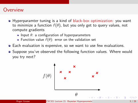
Hyperparamter tuning is a kind of black-box optimization: you wantto minimize a function f (θ), but you only get to query values, notcompute gradients
Input θ: a configuration of hyperparametersFunction value f (θ): error on the validation set
Each evaluation is expensive, so we want to use few evaluations.
Suppose you’ve observed the following function values. Where wouldyou try next?
Roger Grosse CSC321 Lecture 21: Bayesian Hyperparameter Optimization 3 / 25
Overview
You want to query a point which:
you expect to be goodyou are uncertain about
How can we model our uncertainty about the function?
Bayesian regression lets us predict not just a value, but a distribution.That’s what the first half of this lecture is about.
Roger Grosse CSC321 Lecture 21: Bayesian Hyperparameter Optimization 4 / 25
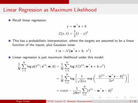
Linear Regression as Maximum Likelihood
Recall linear regression:
y = w>x + b
L(y , t) =1
2(t − y)2
This has a probabilistic interpretation, where the targets are assumed to be a linearfunction of the inputs, plus Gaussian noise:
t | x ∼ N (w>x + b, σ2)
Linear regression is just maximum likelihood under this model:
1
N
N∑i=1
log p(t(i) | x(i);w, b) =1
N
N∑i=1
logN (t(i);w>x + b, σ2)
=1
N
N∑i=1
log
[1√2πσ
exp
(− (t(i) − w>x− b)2
2σ2
)]
= const− 1
2Nσ2
N∑i=1
(t(i) − w>x− b)2
Roger Grosse CSC321 Lecture 21: Bayesian Hyperparameter Optimization 5 / 25

Bayesian Linear Regression
We’re interested in the uncertainty
Bayesian linear regression considers various plausible explanations forhow the data were generated.
It makes predictions using all possible regression weights, weighted bytheir posterior probability.
Roger Grosse CSC321 Lecture 21: Bayesian Hyperparameter Optimization 6 / 25

Bayesian Linear Regression
Leave out the bias for simplicity
Prior distribution: a broad, spherical (multivariate) Gaussian centered atzero:
w ∼ N (0, ν2I)
Likelihood: same as in the maximum likelihood formulation:
t | x,w ∼ N (w>x, σ2)
Posterior:
log p(w | D) = const + log p(w) +N∑i=1
log p(t(i) |w, x(i))
= const + logN (w; 0, ν2I) +N∑i=1
logN (t(i);w>x(i), σ)
= cost− 1
2ν2w>w − 1
2σ2
N∑i=1
(t(i) −w>x(i))2
Roger Grosse CSC321 Lecture 21: Bayesian Hyperparameter Optimization 7 / 25
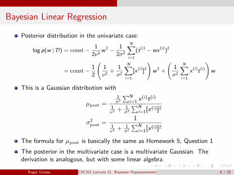
Bayesian Linear Regression
Posterior distribution in the univariate case:
log p(w | D) = const− 1
2ν2w 2 − 1
2σ2
N∑i=1
(t(i) − wx (i))2
= const− 1
2
(1
ν2+
1
σ2
N∑i=1
[x (i)]2)w 2 +
(1
σ2
N∑i=1
x (i)t(i))w
This is a Gaussian distribution with
µpost =1σ2
∑Ni=1 x
(i)t(i)
1ν2 + 1
σ2
∑Ni=1[x (i)]2
σ2post =
11ν2 + 1
σ2
∑Ni=1[x (i)]2
The formula for µpost is basically the same as Homework 5, Question 1
The posterior in the multivariate case is a multivariate Gaussian. Thederivation is analogous, but with some linear algebra.
Roger Grosse CSC321 Lecture 21: Bayesian Hyperparameter Optimization 8 / 25
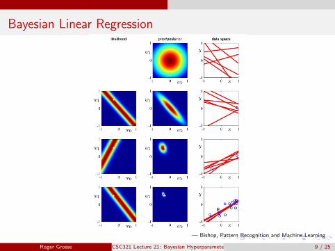
Bayesian Linear Regression
— Bishop, Pattern Recognition and Machine Learning
Roger Grosse CSC321 Lecture 21: Bayesian Hyperparameter Optimization 9 / 25
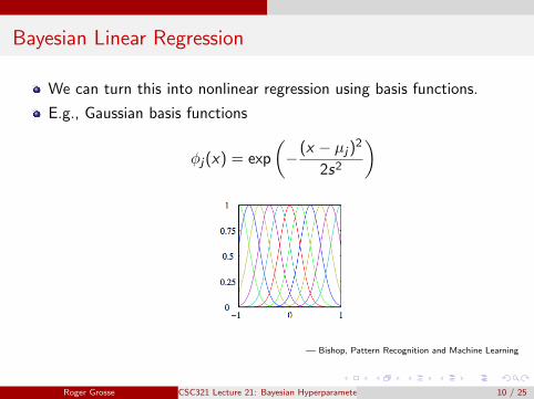
Bayesian Linear Regression
We can turn this into nonlinear regression using basis functions.
E.g., Gaussian basis functions
φj(x) = exp
(−
(x − µj)2
2s2
)
— Bishop, Pattern Recognition and Machine Learning
Roger Grosse CSC321 Lecture 21: Bayesian Hyperparameter Optimization 10 / 25

Bayesian Linear Regression
Functions sampled from the posterior:
— Bishop, Pattern Recognition and Machine Learning
Roger Grosse CSC321 Lecture 21: Bayesian Hyperparameter Optimization 11 / 25
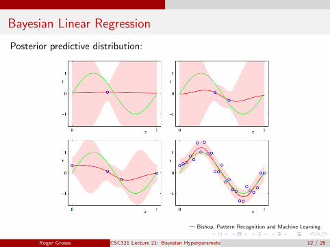
Bayesian Linear Regression
Posterior predictive distribution:
— Bishop, Pattern Recognition and Machine Learning
Roger Grosse CSC321 Lecture 21: Bayesian Hyperparameter Optimization 12 / 25

Bayesian Neural Networks
Basis functions (i.e. feature maps) are great in one dimension, but don’tscale to high-dimensional spaces.
Recall that the second-to-last layer of an MLP can be thought of as afeature map:
It is possible to train a Bayesian neural network, where we define a prior overall the weights for all layers, and make predictions using Bayesian parameterestimation.
The algorithms are complicated, and beyond the scope of this class.
A simple approximation which sometimes works: first train the MLP the
usual way, and then do Bayesian linear regression with the learned features.
Roger Grosse CSC321 Lecture 21: Bayesian Hyperparameter Optimization 13 / 25

Bayesian Optimization
Now let’s apply all of this to black-box optimization. The techniquewe’ll cover is called Bayesian optimization.The actual function we’re trying to optimize (e.g. validation error as afunction of hyperparameters) is really complicated. Let’s approximateit with a simple function, called the surrogate function.After we’ve queried a certian number of points, we can condition onthese to infer the posterior over the surrogate function using Bayesianlinear regression.
Roger Grosse CSC321 Lecture 21: Bayesian Hyperparameter Optimization 14 / 25
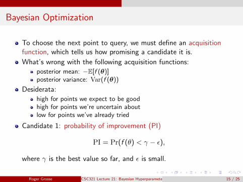
Bayesian Optimization
To choose the next point to query, we must define an acquisitionfunction, which tells us how promising a candidate it is.
What’s wrong with the following acquisition functions:
posterior mean: −E[f (θ)]posterior variance: Var(f (θ))
Desiderata:
high for points we expect to be goodhigh for points we’re uncertain aboutlow for points we’ve already tried
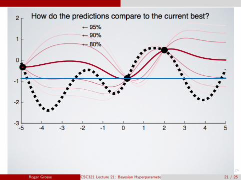
Candidate 1: probability of improvement (PI)
PI = Pr(f (θ) < γ − ε),
where γ is the best value so far, and ε is small.
Roger Grosse CSC321 Lecture 21: Bayesian Hyperparameter Optimization 15 / 25
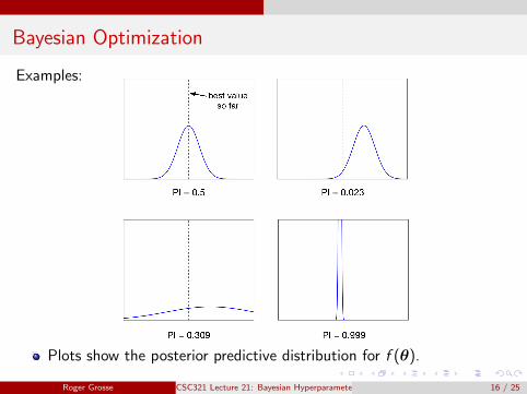
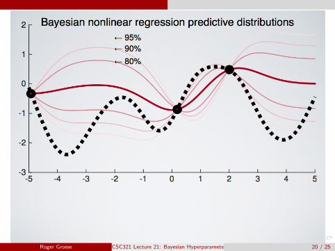
Bayesian Optimization
Examples:
Plots show the posterior predictive distribution for f (θ).
Roger Grosse CSC321 Lecture 21: Bayesian Hyperparameter Optimization 16 / 25
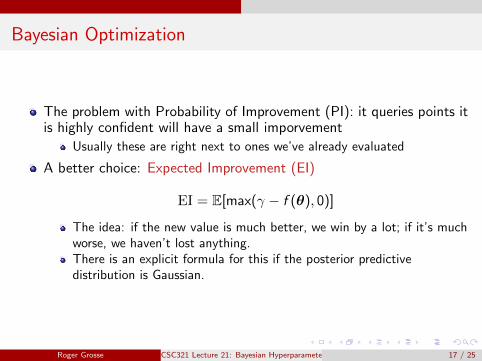
Bayesian Optimization
The problem with Probability of Improvement (PI): it queries points itis highly confident will have a small imporvement
Usually these are right next to ones we’ve already evaluated
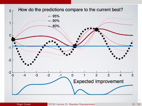
A better choice: Expected Improvement (EI)
EI = E[max(γ − f (θ), 0)]
The idea: if the new value is much better, we win by a lot; if it’s muchworse, we haven’t lost anything.There is an explicit formula for this if the posterior predictivedistribution is Gaussian.
Roger Grosse CSC321 Lecture 21: Bayesian Hyperparameter Optimization 17 / 25

Bayesian Optimization
Examples:
Roger Grosse CSC321 Lecture 21: Bayesian Hyperparameter Optimization 18 / 25

Roger Grosse CSC321 Lecture 21: Bayesian Hyperparameter Optimization 19 / 25
Roger Grosse CSC321 Lecture 21: Bayesian Hyperparameter Optimization 20 / 25
Roger Grosse CSC321 Lecture 21: Bayesian Hyperparameter Optimization 21 / 25
Roger Grosse CSC321 Lecture 21: Bayesian Hyperparameter Optimization 22 / 25
Bayesian Optimization
I showed one-dimensional visualizations, but the higher-dimensionalcase is conceptually no different.
Maximize the acquisition function using gradient descentUse lots of random restarts, since it is riddled with local maximaBayesOpt can be used to optimize tens of hyperparameters.
I’ve described BayesOpt in terms of Bayesian linear regression withbasis functions learned by a neural net.
In practice, it’s typically done with a more advanced model calledGaussian processes, which you learn about in CSC 412.But Bayesian linear regression is actually useful, since it scales better tolarge numbers of queries.
One variation: some configurations can be much more expensive thanothers
Use another Bayesian regression model to estimate the computationalcost, and query the point that maximizes expected improvement persecond
Roger Grosse CSC321 Lecture 21: Bayesian Hyperparameter Optimization 23 / 25
Bayesian Optimization
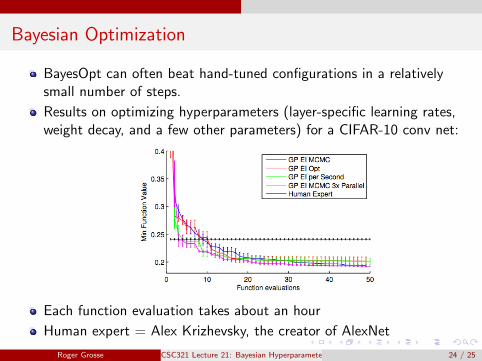
BayesOpt can often beat hand-tuned configurations in a relativelysmall number of steps.
Results on optimizing hyperparameters (layer-specific learning rates,weight decay, and a few other parameters) for a CIFAR-10 conv net:
Each function evaluation takes about an hour
Human expert = Alex Krizhevsky, the creator of AlexNet
Roger Grosse CSC321 Lecture 21: Bayesian Hyperparameter Optimization 24 / 25
Bayesian Optimization
Spearmint is an open-source BayesOpt software package thatoptimizes hyperparameters for you:
https://github.com/JasperSnoek/spearmint
Much of this talk was taken from the following two papers:J. Snoek, H. Larochelle, and R. P. Adams. Practical Bayesianoptimization of machine learning algorithms. NIPS, 2012.
http://papers.nips.cc/paper/
4522-practical-bayesian-optimization-of-machine-learning-algorithms
J. Snoek et al. Scalable Bayesian optimization using deep neuralnetworks. ICML, 2015.
http://www.jmlr.org/proceedings/papers/v37/snoek15.pdf
Roger Grosse CSC321 Lecture 21: Bayesian Hyperparameter Optimization 25 / 25