CSC373: Algorithm Design, Analysis andComplexityFall 2017

Allan Borodin (in collaboration with Rabia Bakhteri and withoccasional guest lectures by Nisarg Shah and Denis Pankratov)

September 13, 2017

1 / 1

Introduction

Course Organization: See General Course Info on course web site:http://www.cs.toronto.edu/∼bor/373f17/

Note: In general we will not post lecture slides and, moreover, wewill not be relying on lecture slides but mainly relying on thewhite/black board. There are (at least) three excellent texts formaterial in this course. We are using CLRS, DPV, and KT. Therewill also be additional material that I will post. I am hoping for amore interactive class with everyone reading the suggested sectionsof these three texts and recommended additional material.

TODO today: We need to assign students to tutorials. We will initiallyuse three tutorial sections assigning students by birthdays: 1-15th of eachmonth (BA 1190), 16-23 (BA 2139) and 24-31 (BA 2145)

2 / 1

What is CSC373?

CSC373 is a “compromise course”. Namely, in the desire to givestudents more choice, there are only two specific courses which arerequired for all CS specialists. Namely we require one “systemscourse” CSC369 and one “theory course” CSC373 whereas in the pastwe required both an algorithms course and a complexity course. Oursolution was to make CSC373 mainly an algorithms course, but toalso include an introduction to complexity theory. DCS also providesa 4th year complexity course CSC465 as well as a more advancedundergraduate algorithms course CSC473.

The complexity part of the course relies on suitable “reductions” (i.e.,converting an instance of a problem A to an instance of problem B).As such, since reductions are algorithms, this is not an unnaturalcombination. The main difference is that we generally use reductionsin complexity theory to provide evidence that something is difficult(rather than use it to derive new algorithms). More on this later.Indeed most algorithm textbooks include NP-completeness.

3 / 1

The dividing line between efficiently computable andNP hardness

Many closely related problems are such that:

One problem has an efficient algorithm (e.g., polynomial time) while avariant becomes (according to “well accepted” conjectures) difficult to

compute (e.g. requiring exponential time complexity).

For example:I Interval Scheduling vs Job Interval SchedulingI Minimum Spanning Tree (MST) vs Bounded degree MSTI MST vs Steiner treeI Shortest paths vs Longest (simple) pathsI 2-Colourability vs 3-Colourability

Our focus is worst case analysis vs peformance “in practice”

4 / 1

Comments and disclaimers on the courseperspective; what this course is and is not about

As this is a required basic course, I am following the perspective ofthe standard CS undergraduate texts. However, I may sometimesintroduce ideas relating to my current research interests.

Most CS undergraduate algorithm courses/texts study the high levelpresentation of algorithms within the framework of basic algorithmicparadigms that can be applied in a wide variety of contexts.

Moreover, the perspective is one of studying “worst case”(adversarial) input instances.

Why not study “average case analysis”

A more applied perspective (i.e., an “algorithmic engineering” coursethat say discusses implementations of algorithms in industrialapplications) is beyond the scope of this course.Why isn’t such a course offered?

5 / 1

Comments and disclaimers on the courseperspective; what this course is and is not about

As this is a required basic course, I am following the perspective ofthe standard CS undergraduate texts. However, I may sometimesintroduce ideas relating to my current research interests.

Most CS undergraduate algorithm courses/texts study the high levelpresentation of algorithms within the framework of basic algorithmicparadigms that can be applied in a wide variety of contexts.

Moreover, the perspective is one of studying “worst case”(adversarial) input instances.Why not study “average case analysis”

A more applied perspective (i.e., an “algorithmic engineering” coursethat say discusses implementations of algorithms in industrialapplications) is beyond the scope of this course.Why isn’t such a course offered?

5 / 1

Comments and disclaimers on the courseperspective; what this course is and is not about

As this is a required basic course, I am following the perspective ofthe standard CS undergraduate texts. However, I may sometimesintroduce ideas relating to my current research interests.

Most CS undergraduate algorithm courses/texts study the high levelpresentation of algorithms within the framework of basic algorithmicparadigms that can be applied in a wide variety of contexts.

Moreover, the perspective is one of studying “worst case”(adversarial) input instances.Why not study “average case analysis”

A more applied perspective (i.e., an “algorithmic engineering” coursethat say discusses implementations of algorithms in industrialapplications) is beyond the scope of this course.

Why isn’t such a course offered?

5 / 1

Comments and disclaimers on the courseperspective; what this course is and is not about

As this is a required basic course, I am following the perspective ofthe standard CS undergraduate texts. However, I may sometimesintroduce ideas relating to my current research interests.

Most CS undergraduate algorithm courses/texts study the high levelpresentation of algorithms within the framework of basic algorithmicparadigms that can be applied in a wide variety of contexts.

Moreover, the perspective is one of studying “worst case”(adversarial) input instances.Why not study “average case analysis”

A more applied perspective (i.e., an “algorithmic engineering” coursethat say discusses implementations of algorithms in industrialapplications) is beyond the scope of this course.Why isn’t such a course offered?

5 / 1

What this course is and is not about (continued)

Our focus is on deterministic algorithms for discrete combinatorial(and some numeric/algebraic) type problems which we study withrespect to sequential time within a von Neumann RAMcomputational model.

Even within theoretical CS, there are many focused courses and textsfor particular subfields. At an advanced undergraduate or graduatelevel, we might have entire courses on for example, randomizedalgorithms, stochastic (i.e., “average case”) analysis, approximationalgorithms, linear programming (and more generally mathematicalprogramming), online algorithms, parallel algorithms, streamingalgorithms, sublinear time algorithms, spectral algorithms (and more,generally algebraic algorithms), geometric algorithms, continuousmethods for discrte problems, genetic algorithms, etc.

6 / 1

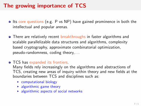
The growing importance of TCS

Its core questions (e.g. P vs NP) have gained prominence in both theintellectual and popular arenas.

There are relatively recent breakthroughs in faster algorithms andscalable parallelizable data structures and algorithms, complexitybased cryptography, approximate combinatorial optimization,pseudo-randomness, coding theory,. . .

TCS has expanded its frontiers.Many fields rely increasingly on the algorithms and abstractions ofTCS, creating new areas of inquiry within theory and new fields at theboundaries between TCS and disciplines such as:

I computational biologyI algorithmic game theoryI algorithmic aspects of social networks

7 / 1

End of introductory comments

I recognize some (many, most?) students may be attending only becauseit is required. You may also be wondering “will I ever use any of thematerial in this course”? or “Why is this course required”?

How many share this sentiment?

Our goal is to instill some more analytical, precise ways of thinking andthis goes beyond the specific course content. The Design and Analysis ofAlgorithms is a required course is almost all North American CS programs.(It probably is also required throughout the world but I know more aboutNorth America.) So the belief that this kind of thinking is useful andimportant is widely accepted. I hope I can make it seem meaningful to younow and not just maybe only 10 years from now.

8 / 1

End of introductory comments

I recognize some (many, most?) students may be attending only becauseit is required. You may also be wondering “will I ever use any of thematerial in this course”? or “Why is this course required”?

How many share this sentiment?

Our goal is to instill some more analytical, precise ways of thinking andthis goes beyond the specific course content. The Design and Analysis ofAlgorithms is a required course is almost all North American CS programs.(It probably is also required throughout the world but I know more aboutNorth America.) So the belief that this kind of thinking is useful andimportant is widely accepted. I hope I can make it seem meaningful to younow and not just maybe only 10 years from now.

8 / 1

End of introductory comments

I recognize some (many, most?) students may be attending only becauseit is required. You may also be wondering “will I ever use any of thematerial in this course”? or “Why is this course required”?

How many share this sentiment?

Our goal is to instill some more analytical, precise ways of thinking andthis goes beyond the specific course content. The Design and Analysis ofAlgorithms is a required course is almost all North American CS programs.(It probably is also required throughout the world but I know more aboutNorth America.) So the belief that this kind of thinking is useful andimportant is widely accepted. I hope I can make it seem meaningful to younow and not just maybe only 10 years from now.

8 / 1

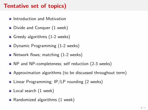
Tentative set of topics)

Introduction and Motivation

Divide and Conquer (1 week)

Greedy algorithms (1-2 weeks)

Dynamic Programming (1-2 weeks)

Network flows; matching (1-2 weeks)

NP and NP-completeness; self reduction (2-3 weeks)

Approximation algorithms (to be discussed throughout term)

Linear Programming; IP/LP rounding (2 weeks)

Local search (1 week)

Randomized algorithms (1 week)

9 / 1

Outline for the course content in Week 1

We will start the course with divide and conquer, a basic algoithmicparadigm that you are familiar with from say CSC236/CSC240, andCSC263/CSC265.The texts contain many examples of divide and conquer as well as how tosolve certain types of recurrences which again you have already seen inprevious courses. So I do not plan to spend too much time on divide andconquer.Here is what we will be doing:(1) An informal statement of the divide and conquer paradigmNote: Like other paradigms we will consider, we do not present aprecise definition for divide and conquer. For our purposes (andthat of the texts), it is a matter of “you know it when you see it”.But if we wanted to say prove that a given problem could not besolved efficiently by a divide and conquer algorithm we would needa precise model.

10 / 1

Outline for Week 1 continued

(2) We will choose a few of the many examples taken mainly from theexamples in texts:

CLRS: maximum subarray, Strassen’s matrix multiplication, quicksort,median and selection in sorted list, dynamic multithreading, the FFTalgorithm, closest pair in R2, sparse cuts in graphs

KT: merge sort, counting imversions, closest pair in R2, integermultiplication, FFT, quicksort, medians and selection

(3) The typical recurrences(4) Comments on choosing the right abstraction of the problem.

11 / 1

The divide and conquer paradigm

As roughly stated in DPV chapter 2, the divide and conquer paradigmsolves a problem by:

1 Dividing the problem into smaller subproblems of the same typeNote: In some cases we have to generalize the given problem so as tolend itself to the paradigm. We will also see this in the dynamicprogramming paradigm.

2 Recursively solving these subproblems

3 Combining the results from the subproblems

12 / 1

Counting inversions from Kevin Wayne’s slides

20

Counting Inversions: Implementation

Pre-condition. [Merge-and-Count] A and B are sorted.

Post-condition. [Sort-and-Count] L is sorted.

Sort-and-Count(L) {

if list L has one element

return 0 and the list L

Divide the list into two halves A and B

(rA, A) ← Sort-and-Count(A)

(rB, B) ← Sort-and-Count(B)

(rB, L) ← Merge-and-Count(A, B)

return r = rA + rB + r and the sorted list L

}

Figure : Counting-inversions from Kevin Wayne’s slides13 / 1

Closest pair in R2 from Kevin Wayne’s slides

33

Closest Pair Algorithm

Closest-Pair(p1, …, pn) {

Compute separation line L such that half the points

are on one side and half on the other side.

δ1 = Closest-Pair(left half) δ2 = Closest-Pair(right half) δ = min(δ1, δ2)

Delete all points further than δ from separation line L

Sort remaining points by y-coordinate.

Scan points in y-order and compare distance between

each point and next 11 neighbors. If any of these

distances is less than δ, update δ.

return δ.}

O(n log n)

2T(n / 2)

O(n)

O(n log n)

O(n)

Figure : Closest pairs from Kevin Wayne’s slides

14 / 1

Recurrences describing divide and conqueralgorithms

From previous courses (and previous examples), we have seen therecurrences describing the divide and conquer algorithms for countinginversions and closest points in R2. NamelyT (n) = 2T (n/2) + O(n) and T (1) = O(1) so thatT (n) = O(n log n).

The next two divide and couquer examples examples result inrecurrences of the form T (n) = aT (n/b) + f (n) for a > b wheref (n) = O(nlogb a−ε) for some ε > 0. so that T (n) = nlogb a.

These are all cases of the so called master theorem

15 / 1

The master theorem

Here is the master theorem as it appears in CLRS

94 Chapter 4 Divide-and-Conquer

The recurrence (4.20) describes the running time of an algorithm that divides aproblem of size n into a subproblems, each of size n=b, where a and b are positiveconstants. The a subproblems are solved recursively, each in time T .n=b/. Thefunction f .n/ encompasses the cost of dividing the problem and combining theresults of the subproblems. For example, the recurrence arising from Strassen’salgorithm has a D 7, b D 2, and f .n/ D ‚.n2/.

As a matter of technical correctness, the recurrence is not actually well defined,because n=b might not be an integer. Replacing each of the a terms T .n=b/ witheither T .bn=bc/ or T .dn=be/ will not affect the asymptotic behavior of the recur-rence, however. (We will prove this assertion in the next section.) We normallyfind it convenient, therefore, to omit the floor and ceiling functions when writingdivide-and-conquer recurrences of this form.

The master theoremThe master method depends on the following theorem.

Theorem 4.1 (Master theorem)Let a ! 1 and b > 1 be constants, let f .n/ be a function, and let T .n/ be definedon the nonnegative integers by the recurrenceT .n/ D aT .n=b/C f .n/ ;

where we interpret n=b to mean either bn=bc or dn=be. Then T .n/ has the follow-ing asymptotic bounds:1. If f .n/ D O.nlogb a!!/ for some constant ! > 0, then T .n/ D ‚.nlogb a/.2. If f .n/ D ‚.nlogb a/, then T .n/ D ‚.nlogb a lg n/.3. If f .n/ D ".nlogb aC!/ for some constant ! > 0, and if af .n=b/ " cf .n/ for

some constant c < 1 and all sufficiently large n, then T .n/ D ‚.f .n//.

Before applying the master theorem to some examples, let’s spend a momenttrying to understand what it says. In each of the three cases, we compare thefunction f .n/ with the function nlogb a. Intuitively, the larger of the two functionsdetermines the solution to the recurrence. If, as in case 1, the function nlogb a is thelarger, then the solution is T .n/ D ‚.nlogb a/. If, as in case 3, the function f .n/is the larger, then the solution is T .n/ D ‚.f .n//. If, as in case 2, the two func-tions are the same size, we multiply by a logarithmic factor, and the solution isT .n/ D ‚.nlogb a lg n/ D ‚.f .n/ lg n/.

Beyond this intuition, you need to be aware of some technicalities. In the firstcase, not only must f .n/ be smaller than nlogb a, it must be polynomially smaller.

16 / 1

Karatsuba’s interger multiplication from KevinWayne’s slides

10

To multiply two n-bit integers a and b:

Add two ½n bit integers.

Multiply three ½n-bit integers, recursively.

Add, subtract, and shift to obtain result.

Theorem. [Karatsuba-Ofman 1962] Can multiply two n-bit integers

in O(n1.585) bit operations.

Karatsuba Multiplication

!

T (n) " T n /2# $( ) + T n /2% &( ) + T 1+ n /2% &( )recursive calls

1 2 4 4 4 4 4 4 4 3 4 4 4 4 4 4 4 + '(n)

add, subtract, shift

1 2 4 3 4 ( T (n) = O(n

lg 3) = O(n

1.585)

!

a = 2n / 2

" a1 + a0

b = 2n / 2

"b1 + b0

ab = 2n" a1b1 + 2

n / 2" a1b0 + a0b1( ) + a0b0

= 2n" a1b1 + 2

n / 2" (a1 + a0 ) (b1 +b0 ) # a1b1 # a0b0( ) + a0b0

1 2 1 33

17 / 1

Strassen’s n × n fast matrix multiplication

This algorithm is described in all the texts. While there is some questionas to when fast matrix multiplicaton (Strassen’s and subsequentasymptotically faster algorithms) has practical application, it plays aseminal role in theoretical computer science.

The standard method to multiply two n× n matrices requires O(n3) scalar(+, ·) operations. There were conjectures (and a published false proof!)that any algorithm for matrix multipication requires O(n3)

Why would you make such a conjecture? And why is this such a seminalresult?

Theorem (Strassen): Matrix multiplcation (over any ring) can berealized in O(nlog2 7) scalar operations.

Furthermore, Strassen shows that matrix inversion for a non-singluarmatrix reduces (and is equivalent) to matrix multiplication.

18 / 1

Strassen’s n × n fast matrix multiplication

This algorithm is described in all the texts. While there is some questionas to when fast matrix multiplicaton (Strassen’s and subsequentasymptotically faster algorithms) has practical application, it plays aseminal role in theoretical computer science.

The standard method to multiply two n× n matrices requires O(n3) scalar(+, ·) operations. There were conjectures (and a published false proof!)that any algorithm for matrix multipication requires O(n3)

Why would you make such a conjecture? And why is this such a seminalresult?

Theorem (Strassen): Matrix multiplcation (over any ring) can berealized in O(nlog2 7) scalar operations.

Furthermore, Strassen shows that matrix inversion for a non-singluarmatrix reduces (and is equivalent) to matrix multiplication.

18 / 1

Strassen’s n × n fast matrix multiplication

This algorithm is described in all the texts. While there is some questionas to when fast matrix multiplicaton (Strassen’s and subsequentasymptotically faster algorithms) has practical application, it plays aseminal role in theoretical computer science.

The standard method to multiply two n× n matrices requires O(n3) scalar(+, ·) operations. There were conjectures (and a published false proof!)that any algorithm for matrix multipication requires O(n3)

Why would you make such a conjecture? And why is this such a seminalresult?

Theorem (Strassen): Matrix multiplcation (over any ring) can berealized in O(nlog2 7) scalar operations.

Furthermore, Strassen shows that matrix inversion for a non-singluarmatrix reduces (and is equivalent) to matrix multiplication.

18 / 1

Strassen’s n × n fast matrix multiplication

This algorithm is described in all the texts. While there is some questionas to when fast matrix multiplicaton (Strassen’s and subsequentasymptotically faster algorithms) has practical application, it plays aseminal role in theoretical computer science.

The standard method to multiply two n× n matrices requires O(n3) scalar(+, ·) operations. There were conjectures (and a published false proof!)that any algorithm for matrix multipication requires O(n3)

Why would you make such a conjecture? And why is this such a seminalresult?

Theorem (Strassen): Matrix multiplcation (over any ring) can berealized in O(nlog2 7) scalar operations.

Furthermore, Strassen shows that matrix inversion for a non-singluarmatrix reduces (and is equivalent) to matrix multiplication.

18 / 1

Strassen’s matrix multiplication continued

The high level idea is conceptually simple. The method is based onStrassen’s insightful (and not simple) discovery that 2× 2 matrixmultiplication can be realized in 7 (not 8) non-commutativemultiplications and 18 additions. (Note: the number of additions will onlyimpact the hidden constant in the “big O” notation and not the matrixmutliplication exponent.)

The insights into the 2× 2 method are beyond the scope of this course solets just see how the n × n result follows. Without loss of generality, letn = 2k for some k .

76 Chapter 4 Divide-and-Conquer

for loop of lines 4–7 computes each of the entries cij , for each column j . Line 5initializes cij to 0 as we start computing the sum given in equation (4.8), and eachiteration of the for loop of lines 6–7 adds in one more term of equation (4.8).

Because each of the triply-nested for loops runs exactly n iterations, and eachexecution of line 7 takes constant time, the SQUARE-MATRIX-MULTIPLY proce-dure takes ‚.n3/ time.

You might at first think that any matrix multiplication algorithm must take !.n3/time, since the natural definition of matrix multiplication requires that many mul-tiplications. You would be incorrect, however: we have a way to multiply matricesin o.n3/ time. In this section, we shall see Strassen’s remarkable recursive algo-rithm for multiplying n ! n matrices. It runs in ‚.nlg 7/ time, which we shall showin Section 4.5. Since lg 7 lies between 2:80 and 2:81, Strassen’s algorithm runs inO.n2:81/ time, which is asymptotically better than the simple SQUARE-MATRIX-MULTIPLY procedure.

A simple divide-and-conquer algorithmTo keep things simple, when we use a divide-and-conquer algorithm to computethe matrix product C D A " B , we assume that n is an exact power of 2 in each ofthe n ! n matrices. We make this assumption because in each divide step, we willdivide n ! n matrices into four n=2 ! n=2 matrices, and by assuming that n is anexact power of 2, we are guaranteed that as long as n # 2, the dimension n=2 is aninteger.

Suppose that we partition each of A, B , and C into four n=2 ! n=2 matrices

A D!

A11 A12

A21 A22

"; B D

!B11 B12

B21 B22

"; C D

!C11 C12

C21 C22

"; (4.9)

so that we rewrite the equation C D A " B as!

C11 C12

C21 C22

"D

!A11 A12

A21 A22

""!

B11 B12

B21 B22

": (4.10)

Equation (4.10) corresponds to the four equationsC11 D A11 " B11 C A12 " B21 ; (4.11)C12 D A11 " B12 C A12 " B22 ; (4.12)C21 D A21 " B11 C A22 " B21 ; (4.13)C22 D A21 " B12 C A22 " B22 : (4.14)Each of these four equations specifies two multiplications of n=2 ! n=2 matricesand the addition of their n=2 ! n=2 products. We can use these equations to createa straightforward, recursive, divide-and-conquer algorithm:

Figure : Viewing an n × n matrix as four n/2× n/2 matrices

19 / 1

Strassen’s matrix multiplication continued

The high level idea is conceptually simple. The method is based onStrassen’s insightful (and not simple) discovery that 2× 2 matrixmultiplication can be realized in 7 (not 8) non-commutativemultiplications and 18 additions. (Note: the number of additions will onlyimpact the hidden constant in the “big O” notation and not the matrixmutliplication exponent.)

The insights into the 2× 2 method are beyond the scope of this course solets just see how the n × n result follows. Without loss of generality, letn = 2k for some k .

76 Chapter 4 Divide-and-Conquer

for loop of lines 4–7 computes each of the entries cij , for each column j . Line 5initializes cij to 0 as we start computing the sum given in equation (4.8), and eachiteration of the for loop of lines 6–7 adds in one more term of equation (4.8).

Because each of the triply-nested for loops runs exactly n iterations, and eachexecution of line 7 takes constant time, the SQUARE-MATRIX-MULTIPLY proce-dure takes ‚.n3/ time.

You might at first think that any matrix multiplication algorithm must take !.n3/time, since the natural definition of matrix multiplication requires that many mul-tiplications. You would be incorrect, however: we have a way to multiply matricesin o.n3/ time. In this section, we shall see Strassen’s remarkable recursive algo-rithm for multiplying n ! n matrices. It runs in ‚.nlg 7/ time, which we shall showin Section 4.5. Since lg 7 lies between 2:80 and 2:81, Strassen’s algorithm runs inO.n2:81/ time, which is asymptotically better than the simple SQUARE-MATRIX-MULTIPLY procedure.

A simple divide-and-conquer algorithmTo keep things simple, when we use a divide-and-conquer algorithm to computethe matrix product C D A " B , we assume that n is an exact power of 2 in each ofthe n ! n matrices. We make this assumption because in each divide step, we willdivide n ! n matrices into four n=2 ! n=2 matrices, and by assuming that n is anexact power of 2, we are guaranteed that as long as n # 2, the dimension n=2 is aninteger.

Suppose that we partition each of A, B , and C into four n=2 ! n=2 matrices

A D!

A11 A12

A21 A22

"; B D

!B11 B12

B21 B22

"; C D

!C11 C12

C21 C22

"; (4.9)

so that we rewrite the equation C D A " B as!

C11 C12

C21 C22

"D

!A11 A12

A21 A22

""!

B11 B12

B21 B22

": (4.10)

Equation (4.10) corresponds to the four equationsC11 D A11 " B11 C A12 " B21 ; (4.11)C12 D A11 " B12 C A12 " B22 ; (4.12)C21 D A21 " B11 C A22 " B21 ; (4.13)C22 D A21 " B12 C A22 " B22 : (4.14)Each of these four equations specifies two multiplications of n=2 ! n=2 matricesand the addition of their n=2 ! n=2 products. We can use these equations to createa straightforward, recursive, divide-and-conquer algorithm:

Figure : Viewing an n × n matrix as four n/2× n/2 matrices

19 / 1

Strassen’s matrix multiplication continued

The high level idea is conceptually simple. The method is based onStrassen’s insightful (and not simple) discovery that 2× 2 matrixmultiplication can be realized in 7 (not 8) non-commutativemultiplications and 18 additions. (Note: the number of additions will onlyimpact the hidden constant in the “big O” notation and not the matrixmutliplication exponent.)

The insights into the 2× 2 method are beyond the scope of this course solets just see how the n × n result follows. Without loss of generality, letn = 2k for some k .

76 Chapter 4 Divide-and-Conquer

for loop of lines 4–7 computes each of the entries cij , for each column j . Line 5initializes cij to 0 as we start computing the sum given in equation (4.8), and eachiteration of the for loop of lines 6–7 adds in one more term of equation (4.8).

Because each of the triply-nested for loops runs exactly n iterations, and eachexecution of line 7 takes constant time, the SQUARE-MATRIX-MULTIPLY proce-dure takes ‚.n3/ time.

You might at first think that any matrix multiplication algorithm must take !.n3/time, since the natural definition of matrix multiplication requires that many mul-tiplications. You would be incorrect, however: we have a way to multiply matricesin o.n3/ time. In this section, we shall see Strassen’s remarkable recursive algo-rithm for multiplying n ! n matrices. It runs in ‚.nlg 7/ time, which we shall showin Section 4.5. Since lg 7 lies between 2:80 and 2:81, Strassen’s algorithm runs inO.n2:81/ time, which is asymptotically better than the simple SQUARE-MATRIX-MULTIPLY procedure.

A simple divide-and-conquer algorithmTo keep things simple, when we use a divide-and-conquer algorithm to computethe matrix product C D A " B , we assume that n is an exact power of 2 in each ofthe n ! n matrices. We make this assumption because in each divide step, we willdivide n ! n matrices into four n=2 ! n=2 matrices, and by assuming that n is anexact power of 2, we are guaranteed that as long as n # 2, the dimension n=2 is aninteger.

Suppose that we partition each of A, B , and C into four n=2 ! n=2 matrices

A D!

A11 A12

A21 A22

"; B D

!B11 B12

B21 B22

"; C D

!C11 C12

C21 C22

"; (4.9)

so that we rewrite the equation C D A " B as!

C11 C12

C21 C22

"D

!A11 A12

A21 A22

""!

B11 B12

B21 B22

": (4.10)

Equation (4.10) corresponds to the four equationsC11 D A11 " B11 C A12 " B21 ; (4.11)C12 D A11 " B12 C A12 " B22 ; (4.12)C21 D A21 " B11 C A22 " B21 ; (4.13)C22 D A21 " B12 C A22 " B22 : (4.14)Each of these four equations specifies two multiplications of n=2 ! n=2 matricesand the addition of their n=2 ! n=2 products. We can use these equations to createa straightforward, recursive, divide-and-conquer algorithm:

Figure : Viewing an n × n matrix as four n/2× n/2 matrices

19 / 1

Strassen’s matrix multiplication continued

Since matrices are a non commutative ring (i.e., matrix multiplication isnot commutative), the 2× 2 result can be applied so that an n × nmutilpication can be realized in 7 n/2× n/2 matrix multiplications (and18 matrix additions).

Since matrix addition uses only O(n2) scalar operations, the number T (n)of scalar opeations is determined by the recurrence :

T (n) = 7 ∗ T (n/2) + O(n2) with T (1) = 1.

This implies the stated result that T (n) = O(nlog2 7).

20 / 1

Strassen’s matrix multiplication continued

Since matrices are a non commutative ring (i.e., matrix multiplication isnot commutative), the 2× 2 result can be applied so that an n × nmutilpication can be realized in 7 n/2× n/2 matrix multiplications (and18 matrix additions).

Since matrix addition uses only O(n2) scalar operations, the number T (n)of scalar opeations is determined by the recurrence :

T (n) = 7 ∗ T (n/2) + O(n2) with T (1) = 1.

This implies the stated result that T (n) = O(nlog2 7).

20 / 1

Other examples of the master theorem

There are a few other cases of the master theorem that often occur. Wewill assume that T (1) = O(1).

The recurrence T (n) = 2T (n/2) + O(1) and T (1) = O(1) impliesT (n) = O(n)A not so useful example: finidng the maximum element in anunsorted list.Somewhat perhaps more useful is to find the minimum and maximumelement in d3n2 e comparisons.

The recurrence T (n) = T (n/b) + O(n) for b > 1 impliesT (n) = O(n).For an example, see exercise 4-5 in CLRS (page 109). Later we willdiscuss how to find the median element in an unsorted list in O(n).

The recurrence T (n) = T (n/b) + O(1) for b > 1 impliesT (n) = O(log n).The standard binary search in a sorted list is a typical example.

21 / 1

What has to be proven?

In general, when analyzing an algorithm, we have to do two basic things:

1 Prove coorectnesss; that is, that the algorithm realizes the requiredproblem specification. For example, for Strassen’s matrixmultiplication, it must be shown that the output matrix is theproduct of the two input matrices. For the closest pair problem weneed to prove that the output is the closest pair of points; that is,that an optimal solution was obtained. Later, when consideringapproximation algorithms, we need to prove that the algorithmproduces a feasible solution within some factor of an optimal solution.

2 Analyze the complexity of the algorithm in terms of the inputparameters of the problem. For us, we will mainly be interested in the(sequential) time of the algorithm as a function T () of the “size” ofthe input representation. For example, in n × n matrix multiplication,the usual measure of “size” is the size n of the matrices. But if wereconsidering the multiplication of Am,n · Bn,p, we would want toanalyze the time complexity T (m, n, p).

22 / 1

More on compelxity analysis

For divide and conquer, we analyze the complexity by establishing arecurrence and then solving that recurrence. For us, the recurrencesare usually solved by the master theorem. In fact, if we know thedesired time bound, we can sometimes guess a suitable recurrencewhich may suggest a framework for a possible solution.There are other important complexity measures besides sequentialtime, including parallel time (if we are in a model of parallelcomputation) and memory space.For much of our algorithm analysis (as in all the previous examplesexcept integer multiplication), we are assumiung a random accessmodel and counting the number of machine operations (e.g.,comparisons, arithmetic operations) ignoring representation issues(e.g., the number of bits or digits in the matrix entries, or therepresentation of the “real numbers” in the closest pair problem). Forinterger multiplcation, we measured the “size” of the inputrepresentation in terms of the number of bits or digits of the twonumbers.

23 / 1

Looking ahead to complexity theory

When we get to complexity theory, the standard measure is the nunber ofbits (or digits) in the representation of the inputs. In particular, whendiscussing the “P vs NP issue and NP completeness, we assume that wehave string (o0ver some finite alphabet) representation of the inputs. (Wewill not usually have to worry about the size of the output.)

This makes sense as for example, in integer factoring (the basis for RSAcryptography) it would not make good sense to measure complexity of thevalue x of the number being factored but rather we need to measurecompexity as a function of the number of bits (or digits) to represent x .Why?

This distinction (between the value of say an integer and its representationlength) will also become important when we discuss the knapsack problemin the context of dynamic programming.

24 / 1

Looking ahead to complexity theory

When we get to complexity theory, the standard measure is the nunber ofbits (or digits) in the representation of the inputs. In particular, whendiscussing the “P vs NP issue and NP completeness, we assume that wehave string (o0ver some finite alphabet) representation of the inputs. (Wewill not usually have to worry about the size of the output.)

This makes sense as for example, in integer factoring (the basis for RSAcryptography) it would not make good sense to measure complexity of thevalue x of the number being factored but rather we need to measurecompexity as a function of the number of bits (or digits) to represent x .Why?

This distinction (between the value of say an integer and its representationlength) will also become important when we discuss the knapsack problemin the context of dynamic programming.

24 / 1