CSWA: Aggregation-Free Spatial-Temporal Community Sensing

Jiang Bian∗, Haoyi Xiong∗, Yanjie Fu, and Sajal K. DasMissouri University of Science and Technology, United States

*Equal Contribution

Abstract

In this paper, we present a novel community sensing paradigmCSWA –Community Sensing Without Sensor/Location DataAggregation. CSWA is designed to obtain the environmentinformation (e.g., air pollution or temperature) in each subareaof the target area, without aggregating sensor and location datacollected by community members. CSWA operates on top ofa secured peer-to-peer network over the community membersand proposes a novel Decentralized Spatial-Temporal Com-pressive Sensing framework based on Parallelized StochasticGradient Descent. Through learning the low-rank structure viadistributed optimization, CSWA approximates the value ofthe sensor data in each subarea (both covered and uncovered)for each sensing cycle using the sensor data locally stored ineach member’s mobile device. Simulation experiments basedon real-world datasets demonstrate that CSWA exhibits lowapproximation error (i.e., less than 0.2◦C in city-wide temper-ature sensing task and 10 units of PM2.5 index in urban airpollution sensing) and performs comparably to (sometimesbetter than) state-of-the-art algorithms based on the data ag-gregation and centralized computation.

IntroductionSpatial-temporal community sensing is an efficient paradigmthat leverages the mobile sensors of community members tomonitor the spatial-temporal phenomena in the environment,such as air pollution or temperature. According to (Zhang etal. 2014a), there are two major roles in community sensing– the organizer and the participants – where the former isthe individual or organization that creates the sensing task,recruits participants and collects the sensor data, while thelatter (i.e., participants) involve in the sensing task and pro-vide the sensing data. Frequently, the organizer pursues ahigh (or even full) spatial-temporal coverage of the collectedsensor data. However incentives (e.g., monetary rewards)and the threats to privacy (e.g., exposing real-time locations)are two major concerns that may affect the willingness of theparticipants to join a community sensing task.

In addition to the community sensing paradigm, a wide-spectrum of applications, ranging from vehicle traffic moni-toring (Ji, Zheng, and Li 2016; Yoon, Noble, and Liu 2007;Herring et al. 2010; Hachem, Pathak, and Issarny 2013;

Copyright c© 2018, Association for the Advancement of ArtificialIntelligence (www.aaai.org). All rights reserved.

Pan et al. 2013) to air quality sensing (Aberer et al. 2010) andurban noise monitoring (Liu et al. 2014), have been proposedto efficiently monitor the environment of a large area throughaggregating the real-time sensor and location data from theparticipants. Such applications use spatial-temporal cover-age as the metric for overall task performance. Specifically,to characterize spatial-temporal coverage, the target area issplit into subareas and the sensing duration is divided intoa sequence of equal-length sensing cycles. In this way, thefraction of subareas covered by at least one sensor reading ineach cycle is used to measure the spatial-temporal coverage.

For example, (Xiong et al. 2015; Sheng, Tang, and Zhang2012) proposed to use the full spatial-temporal coverageas the criterion of the participants selection for commu-nity sensing, while (Zhang et al. 2014b; Hachem, Pathak,and Issarny 2013) studied the partial spatial-temporal cov-erage as the objectives of the optimization for budget-constrained participant selection. With the sensor data thatpartially covers the target area, (Wang et al. 2015; 2016a;2017b) proposed compressive community sensing, which iscapable of recovering the missing sensor data of the uncov-ered subareas from the data collected. Through the compres-sive community sensing, it is possible to accurately monitorthe target area with even lower spatial-temporal coverage,thus resulting in reduced incentive consumption and fewerparticipants involved.

Though compressive community sensing can effectivelyreduce the required incentives and participants, it still ag-gregates the real-time location and sensor data from eachparticipant, so as to first identify the covered subareas, fillwith collected data, and then recover the missing data forthe rest. To protect the location privacy of participants, thesame of group of researchers (Wang et al. 2017a; 2016b) pro-posed to leverage the Differential Geo-Obfuscation to replaceeach participants’ real-time location with a "mock" locationwhile insuring the recovery accuracy. With the DifferentialGeo-Obfuscation, the participants’ locations are expected tobe well obfuscated; however, it is still possible to attack theparticipant’s location when certain prior knowledge is leaked.Thus, in our research, to further protect the real-time locationprivacy, we propose a novel Aggregation-Free CompressiveCommunity Sensing framework, with following assumptions:

• Assumption I: the organizer is NOT allowed to collect thereal-time location or the sensor data from any participant;

arX

iv:1

711.

0571

2v1

[cs

.LG

] 1

5 N

ov 2

017

• Assumption II: Each participant covers one or multiplesubareas in each sensing cycles with his/her mobility, whilethe location and sensor data is locally stored on his/hermobile device without raw location/sensor data sharing.Thus, to achieve the above goals, we propose a novel

community sensing paradigm CSWA. Specifically, CSWAfirst establishes secured peer-to-peer network connectionsbetween each pairs participants. Then, CSWA proposes adecentralized non-negative matrix factorization algorithmbased on Parallelized Stochastic Gradient Descent frame-work. Through learning the low-rank structure via distributedoptimization, CSWA approximates the value of sensor datain each subarea (both covered and uncovered) for each sens-ing cycle using the sensor data that are locally stored in eachparticipant’s mobile device.

The contributions of this paper are as follows:• We propose a novel community sensing frameworkCSWA, which is used to recover the environmental infor-mation in subareas, without aggregating sensor and loca-tion data from the community members who partially coverthe target area. To the best of our knowledge, this paper isthe first work that studies the problem of aggregation-freecommunity sensing, by addressing the location privacy,distributed computing and optimization issues.

• To enable community sensing without location/sensordata aggregation, CSWA proposes a novel decentralizedspatial-temporal compressive sensing framework that re-covers the spatial-temporal information via decentralizedNon-negative Matrix Factorization (NMF).The proposedsolution operates on top of the parallelized stochastic gra-dient descent, which minimizes the loss function of NMFthrough secure Peer-to-Peer (P2P) message-passing overcommunity members. The algorithm analysis shows thatthe proposed solution can efficiently approximates to thecentralized NMF with the tolerable worst-case communi-cation complexity.

• We evaluate CSWA using two large real-world datasets(i.e., temperature and air pollution). The experimental re-sults demonstrate that CSWA tightly approximates to thestate-of-the-art algorithms based on the data aggregationwith centralized computation, and it outperforms the restbaselines with significant margin.

The rest of the paper is organized as follows. In the Pre-liminaries and Problem formulation section, we review thecompressive community sensing and the matrix factoriza-tion approach. Then we introduce the parallelized stochasticgradient descent and present the problem formulation. Inthe Frameworks and Algorithms section, we propose frame-work of CSWA and present the algorithms in details. Inthe Experiments section, we evaluate CSWA on real-worlddatasets and compare it with baseline algorithms. Finally, inthe Conclusion section, we summarize the work in this paper.

Preliminaries and Problem FormulationIn this section, we first briefly introduce the previous workon the compressive community sensing. Then, we formulatethe problem of our research.

Compressive Community SensingTo derive the target full sensing matrix from partially col-lected sensing readings, the compressive community sens-ing (Wang et al. 2015; 2016a) is commonly considered to bean effective approach, which consists of two parts:

Sensing Data Aggregation – Given the target region split-ting into a set of subareas (denoted as S) and a set of mparticipants, in order to obtain the full picture of the targetregion for each sensing cycle (e.g., the tth cycle), the Com-pressive Community Sensing system first collects the sensingdata from all participants. Specifically, the subareas coveredby the jth participant in the tth sensing cycle (t ∈ T ) isdenoted as St

j ⊂ S. Thus, the overall coverage in the sensingcycle t can be denoted as St = St

1 ∪ St2 ∪ ... ∪ St

m. Due tothe limited mobility of each participant and limited numberof participants involved, the overall coverage can usually in-clude a subset of subareas, i.e., St ⊆ S. Given the collectedsensing data, the compressive community sensing system ag-gregates the data and assigns each covered subarea an uniquesensor data value. For example, if multiple sensor data val-ues are collected (from multiple participants) that covers thesame subarea in a sensing cycle, the averaged value would beused as the value of such subarea in the sensing cycle. In thisway, each subarea s ∈ St has been covered with one sensordata value, through data aggregation, and the compressivecommunity sensing system needs to infer the missing sensordata of the subareas in S\St to obtain the sensor data of thewhole target area.

Missing Data Inference – Given the aggregated sensordata of the covered subareas (St), there exists a wide-rangeof inferring techniques to infer the missing data of the uncov-ered subareas, such as expectation maximization (Schneider2001) and singular spectrum analysis (Kondrashov and Ghil2006). One of the powerful approach is the spatial-temporalcompressive sensing (Kong et al. 2013; Zhang et al. 2009).The essential idea of this approach is based on the nonneg-ative matrix factorization (NMF) (Lee and Seung 2001;Mao and Saul 2004). Given the aggregated sensor data ofrecent sensing cycles (the number of recent sensing cyclesused for NMF is denoted as w), this approach first sorts thesubareas using their indices from 1 . . . to |S|, then maps thedata into a |S| × w matrix denote as R, where the elementRa,t ( 1 ≤ a ≤ |S| and 1 ≤ t ≤ w) refers to the aggregatedsensing value of the ath subarea and tth sensing cycle (in thewindow). To recover the missing values in R, this approachobtains two non-negative matrix factors P ∈ R|S|×l andQ ∈ Rl×w such that R ≈ PQ, through NMF, where l standsfor the Size of Latent Space of NMF.

Typically, there are four key factors affecting the perfor-mance of the compressive community sensing: (1) The Num-ber of Subareas that each participant covers in each sensingcycle; (2) The Number of Participants (m) which, togetherwith the number of subareas per participant, can determinethe coverage of collected sensor data; (3) The Size of Windows(w) that refers to the number of past sensing cycles used formatrix recovery (i.e., the width of the matrix for matrix com-pletion); (4) The Size of Latent Space (l) that determines the

1 2 3 4 5

1

2

3

4

5

1 2 3 4 5

1

2

3

4

5

1 2 3 4 5

1

2

3

4

5

1 2 3 4 5

1

2

3

4

5

1 2 3 4 5

1

2

3

4

5

1 2 3 4 5

1

2

3

4

5

C

1 2 3 4 5

1

2

3

4

5

1 2 3 4 5

1

2

3

4

5

D

A B

C D

A B

C D

Time Slots (Cycles)

Lo

cati

on

s

Covered Cell

Uncovered Cell

B A

RPQ

P

Q

&

Participant

&

Organizer

Message Passing

(Batch 1)

Message Passing

(Batch 2) Recovered Cell

(a) Phase I: Secured P2P Network Estab-lishment and Initialization

1 2 3 4 5

1

2

3

4

5

1 2 3 4 5

1

2

3

4

5

1 2 3 4 5

1

2

3

4

5

1 2 3 4 5

1

2

3

4

5

1 2 3 4 5

1

2

3

4

5

1 2 3 4 5

1

2

3

4

5

C

1 2 3 4 5

1

2

3

4

5

1 2 3 4 5

1

2

3

4

5

D

A B

C D

A B

C D

Time Slots (Cycles)

Subareas

Covered Cell

Uncovered Cell

B A

RPQ

P

Q

&

Participant

&

Organizer

(b) Phase II: Distributed CompressiveCommunity Sensing over Secured P2P

1 2 3 4 5

1

2

3

4

5

1 2 3 4 5

1

2

3

4

5

1 2 3 4 5

1

2

3

4

5

1 2 3 4 5

1

2

3

4

5

1 2 3 4 5

1

2

3

4

5

1 2 3 4 5

1

2

3

4

5

C

1 2 3 4 5

1

2

3

4

5

1 2 3 4 5

1

2

3

4

5

D

A B

C D

A B

C D

Time Slots (Cycles)

Lo

cati

on

s

Covered Cell

Uncovered Cell

B A

RPQ

P

Q

&

Participant

&

Organizer

Message Passing

(Batch 1)

Message Passing

(Batch 2) Recovered Cell

(c) Phase III: Spatial-Temporal Data Recovery

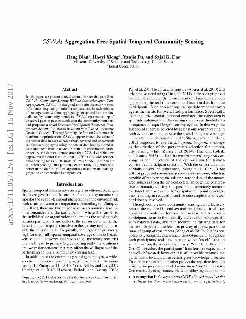
Figure 1: Overall Framework of CSWArank of matrices for low-rank matrix recovery/completion.

Problem FormulationGiven a set of participants, where each participant’s mobiledevice stores the raw sensor data locally (without raw datasharing), our proposed work intends to recover the sensingdata of the target area while assuming that the organizer is notallowed to aggregate the sensor data from any participants.Specifically, we make following assumptions:

• For all the sensing cycles in T and subareas in S, thereexists an unknown spatial-temporal sensor data matrix R∗

(R∗ ∈ R|S|×T ), where each element R∗a′,t′ (1 ≤ a′ ≤ |S|and 1 ≤ t′ ≤ |T |) refers to the real value of sensor data inthe corresponding subarea a′ and sensing cycle t′.

• In each sensing cycle (e.g., the tth cycle), each participant(e.g., the jth participant) covers a subset of subareas (i.e.,Stj ⊆ S) in the target area. Thus, all the collected sen-

sor data from the 1st to the tth sensing cycle of the jth

participant can be represented as a matrix Rj ∈ R|S|×t,where each element refers to the value of the sensor datacollected in the corresponding subarea and cycle. Notethat, to protect the location privacy, Rj is not known bythe organizer.

• We denote the value of the sensor data collected by the jth

participant in sensing cycle t at subarea a as Rja,t. Each

sensor datum obtained is assumed to be the true value with(unknown) random noise, i.e., Rj

a,t = R∗a,t + εja,t. Forany two participants (i.e., the jth and kth participants),they might cover the same subarea (say, atj ∩ St

k 6= ∅ ispossible), but are with different sensor data value obtained,due to the noise.

Our problem is that, in each sensing cycle t, with Rj (1 ≤j ≤ N ) locally stored on each participant’s device, thereneeds to estimate R̂a,t to

minimize|S|∑

a=1

(R̂a,t −R∗a,t)2 for 1 ≤ t ≤ T,

while ensuring that the organizer is prohibited to aggregateRj from any participant and the raw sensor/location datasharing is not allowed between the participants.

Framework and AlgorithmsIn this section, we present the proposed framework ofCSWA and the underlying algorithms. Specifically, we in-troduce a novel Decentralized Spatial-Temporal CompressiveSensing framework based on Parallelized Stochastic GradientDescent.

Framework DesignBefore elaborating the proposed framework and algorithms,we make the following settings: (1) In order to simulate asecure peer-to-peer network over the community members,we define a set of participants, where these participants canreceive or send messages (factor matrices) to each other trust-fully and randomly; (2) When passing the message betweentwo participants, the receiver can not send the updated ma-trix factors back to the sender, while the sender can easilyrecover the receiver’s local sensing data by recalculating thereturn messages; (3) The organizer can only receive or accessthe related message when the updates (message passing) arefinished. In this way, the private information such as real-time locations of the participants in each sensing cycle canbe protected from the organizer.

The overall framework of CSWA consists of the followingthree phases (as illustrated in Figure.1):

Phase I: Secure P2P Network Establishment and Initial-izationPrior to initializing the batch on the organizer, we first estab-lish a secure peer-to-peer (P2P) network among m partici-pants, while all the collected sensor data on the jth participantare mapped to a local data matrix Rj . Then, as shown inAlgorithm. 1, CSWA randomly picks a set of participantswhich is the batch (denoted as the set Lwith sizeN ) from thesecure network of m participants. Next, given the target datamatrix R ∈ R|S|×w, CSWA extracts the row and columnnumber of R to construct the initial matrix factors P̂ and Q̂on the organizer. Specifically, P̂j is generated by a |S| × lGaussian Random Matrix on the jth participant. Similarly,Q̂j is generated by a l × w Gaussian Random Matrix on thesame jth participant. To avoid the aforementioned messagetransferring back between two participants, we initialize acounter i to record passing times (iterations) among partici-pants and set jp to mark the last participant’s index, where

Algorithm 1: Initializing Batch and Matrix Factors(P̂ , Q̂) on Organizer

Data:R|S|×w — the target data matrixParameter:/* Subareas covered by per participant */

|S|— the maximum numbers of subareasw — the size of windowsl — the size of latent spacebegin

/* Predefine a set of participants */

Randomly Draw N Participants into Set L/* L = {I1, I2, ..., IN} */

for each Ij ∈ L do/* Initialize matrix factors P,Q on Ij */

P̂j ← |S| × l Gaussian Random MatrixQ̂j ← l × w Gaussian Random Matrix/* Initialize the counter and the previous

participant index */

SEND (P̂j , Q̂j ,0,null) to L;end

end

the (i, jp) will be transferred along with the updated matrixfactors so that the participant who receives the message canrandomly select the next one excluding participant jp. Whenthe initialization ends, each participant (Ij) in the predefinedset L (batch) will be assigned a pair of starting matrix factorsP̂j and Q̂j .

Phase II: Distributed Compressive Community Sensingvia Parallelized Low-Rank ApproximationGiven the mapped local data matrix Rj on jth participant,CSWA intends to approximate the optimal estimation ofmatrix factors P̂j and Q̂j via parallelized stochastic gradientdescent on top of non-negative matrix factorization algorithm.Specifically, the initialized (P̂j , Q̂j ,0,null) has been allo-cated on the jth participant, where 0 refers to the fact thatno update has been executed and "null" refers to there is noprevious participant (coming from the organizer) which hasupdated the matrix factors (the index of previous participantis empty). Then the algorithm processes the updating task oneach participant from the predefined batch (L) in parallel.

Suppose two dense matrix factors are P ∈ R|S|×l andQ ∈ Rl×w, the target minimization loss function over mparticipants through parallelized stochastic gradient descentis as follow:

P̂ , Q̂← argminP∈R|S|×l,Q∈Rl×w

{1

m

m∑

j=1

∥∥Fj ◦ (Rj − PQ)∥∥2F

+λP ‖P‖2F + λQ ‖Q‖2F

},

(1)where l is the size of latent space, "◦" means element-wisematrix multiplication, ‖·‖F is the Frobenius norm, λP andλQ are regularization parameters. Particularly, parallellystarting on each participant Ij , Algorithm. 2 first receivesthe input (P̂j , Q̂j) from the last involved participant in the

Algorithm 2: Parallelized Optimization on the jth

ParticipantData:Rj — the local data matrix on the jth participantFj — the filter matrix on the jth participantParameter:i — the number iterationsjp, j — the index of previous and current participantη — step size∆min — the minimum allowed perturbationtmax — the maximum number of allowed updatesλP , λQ — regularization parameter on P and Q matricesbegin

/* On receiving the message from the previous

participant */

RECEIVE (P̂j , Q̂j , t, jp)/* Noting that “A ◦ B" means element-wise matrix

multiplication */

gp ← (Fj ◦ (Rj − P̂jQ̂j))Q̂Tj − λP · P̂j

gq ← P̂Tj (Fj ◦ (Rj − P̂jQ̂j))− λQ · Q̂j

P̂j ← P̂j − η · gpQ̂j ← Q̂j − η · gq/* Set the negative elements to zero */

P̂j , Q̂j ← Truncate(P̂j , Q̂j)i← i+ 1/* Checking convergence conditions */

∆ = max{|gp|∞ , |gq|∞

}

if ∆ ≥ ∆max AND i ≤ tmax then/* Not converged, continuing the algorithm */

jnext← Draw a random number from 1 to mexcept jp;

SEND (P̂j , Q̂j , i, j) to the jthnext Participant;else

/* Converged, find out the optimal estimates

*/

SEND (P̂j , Q̂j) to the Organizer;end

end

secure network (or initialized from the organizer in the firstrun). Next it updates the (P̂j , Q̂j) using the mapped localdata matrix Rj with the missing-value filter matrix Fj , andrandomly picks up the next participant except the previousone (jp) from the secure participants network and sends theupdated (P̂j , Q̂j) to this chosen participant. The matrix Fj

is a matrix filling with 0 (missing) and 1 (collected) whichcan set the missing elements in matrix Rj to zero by theelement-wise multiplication. We mainly use it to preventthe missing value in the local data matrix Rj from affectingthe gradient updating in (P̂j , Q̂j). In addition, we leveragethe Truncate() function, where the negative values in matrixfactors (P̂j , Q̂j) will be set to zero, then ensuring the non-negativeness of (P̂j , Q̂j) when finishing each update.

Algorithm. 2 keeps picking up the next participant forupdating, until the times of updates i exceeds the maximalnumber of updates, or the updating process converges (i.e.,max

{|gp|∞ , |gq|∞

}≤ ∆max). Similar procedures are

starting on each participant Ij and the related matrix fac-

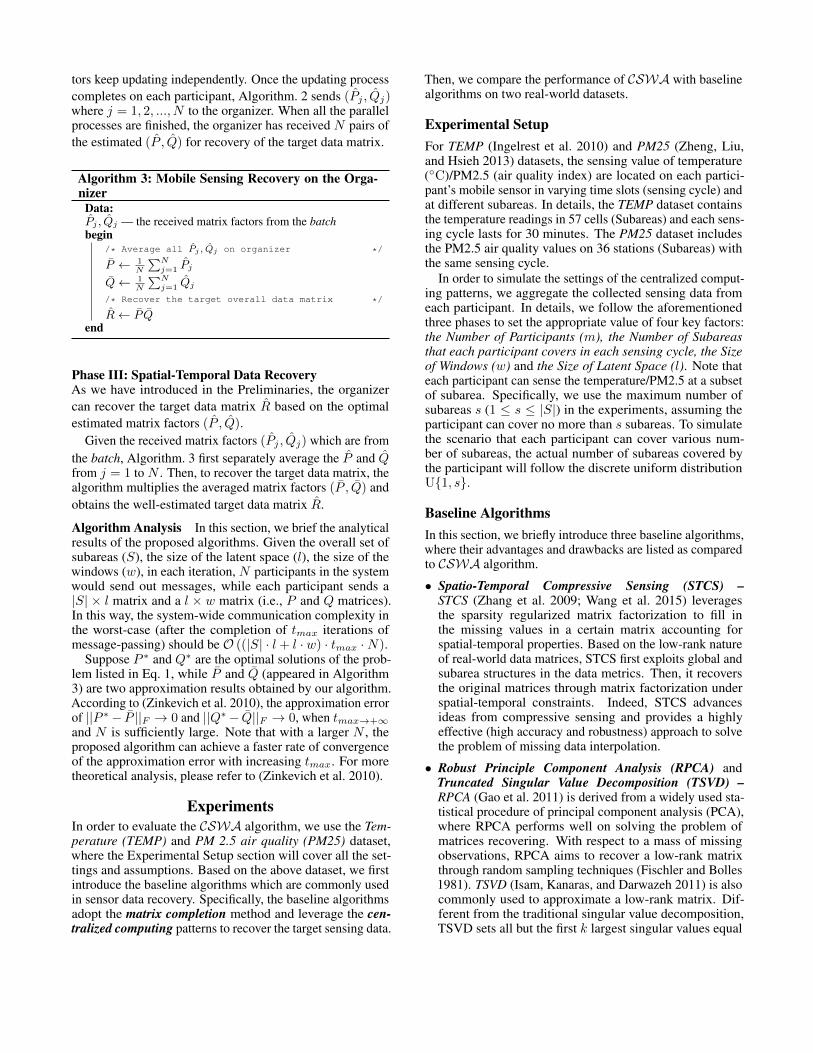
tors keep updating independently. Once the updating processcompletes on each participant, Algorithm. 2 sends (P̂j , Q̂j)where j = 1, 2, ..., N to the organizer. When all the parallelprocesses are finished, the organizer has received N pairs ofthe estimated (P̂ , Q̂) for recovery of the target data matrix.

Algorithm 3: Mobile Sensing Recovery on the Orga-nizer

Data:P̂j , Q̂j — the received matrix factors from the batchbegin

/* Average all P̂j , Q̂j on organizer */

P̄ ← 1N

∑Nj=1 P̂j

Q̄← 1N

∑Nj=1 Q̂j

/* Recover the target overall data matrix */

R̂← P̄ Q̄end

Phase III: Spatial-Temporal Data RecoveryAs we have introduced in the Preliminaries, the organizercan recover the target data matrix R̂ based on the optimalestimated matrix factors (P̂ , Q̂).

Given the received matrix factors (P̂j , Q̂j) which are fromthe batch, Algorithm. 3 first separately average the P̂ and Q̂from j = 1 to N . Then, to recover the target data matrix, thealgorithm multiplies the averaged matrix factors (P̄ , Q̄) andobtains the well-estimated target data matrix R̂.

Algorithm Analysis In this section, we brief the analyticalresults of the proposed algorithms. Given the overall set ofsubareas (S), the size of the latent space (l), the size of thewindows (w), in each iteration, N participants in the systemwould send out messages, while each participant sends a|S| × l matrix and a l × w matrix (i.e., P and Q matrices).In this way, the system-wide communication complexity inthe worst-case (after the completion of tmax iterations ofmessage-passing) should be O ((|S| · l + l · w) · tmax ·N).

Suppose P ∗ and Q∗ are the optimal solutions of the prob-lem listed in Eq. 1, while P̄ and Q̄ (appeared in Algorithm3) are two approximation results obtained by our algorithm.According to (Zinkevich et al. 2010), the approximation errorof ||P ∗− P̄ ||F → 0 and ||Q∗− Q̄||F → 0, when tmax→+∞and N is sufficiently large. Note that with a larger N , theproposed algorithm can achieve a faster rate of convergenceof the approximation error with increasing tmax. For moretheoretical analysis, please refer to (Zinkevich et al. 2010).

ExperimentsIn order to evaluate the CSWA algorithm, we use the Tem-perature (TEMP) and PM 2.5 air quality (PM25) dataset,where the Experimental Setup section will cover all the set-tings and assumptions. Based on the above dataset, we firstintroduce the baseline algorithms which are commonly usedin sensor data recovery. Specifically, the baseline algorithmsadopt the matrix completion method and leverage the cen-tralized computing patterns to recover the target sensing data.

Then, we compare the performance of CSWA with baselinealgorithms on two real-world datasets.

Experimental SetupFor TEMP (Ingelrest et al. 2010) and PM25 (Zheng, Liu,and Hsieh 2013) datasets, the sensing value of temperature(◦C)/PM2.5 (air quality index) are located on each partici-pant’s mobile sensor in varying time slots (sensing cycle) andat different subareas. In details, the TEMP dataset containsthe temperature readings in 57 cells (Subareas) and each sens-ing cycle lasts for 30 minutes. The PM25 dataset includesthe PM2.5 air quality values on 36 stations (Subareas) withthe same sensing cycle.

In order to simulate the settings of the centralized comput-ing patterns, we aggregate the collected sensing data fromeach participant. In details, we follow the aforementionedthree phases to set the appropriate value of four key factors:the Number of Participants (m), the Number of Subareasthat each participant covers in each sensing cycle, the Sizeof Windows (w) and the Size of Latent Space (l). Note thateach participant can sense the temperature/PM2.5 at a subsetof subarea. Specifically, we use the maximum number ofsubareas s (1 ≤ s ≤ |S|) in the experiments, assuming theparticipant can cover no more than s subareas. To simulatethe scenario that each participant can cover various num-ber of subareas, the actual number of subareas covered bythe participant will follow the discrete uniform distributionU{1, s}.

Baseline AlgorithmsIn this section, we briefly introduce three baseline algorithms,where their advantages and drawbacks are listed as comparedto CSWA algorithm.

• Spatio-Temporal Compressive Sensing (STCS) –STCS (Zhang et al. 2009; Wang et al. 2015) leveragesthe sparsity regularized matrix factorization to fill inthe missing values in a certain matrix accounting forspatial-temporal properties. Based on the low-rank natureof real-world data matrices, STCS first exploits global andsubarea structures in the data metrics. Then, it recoversthe original matrices through matrix factorization underspatial-temporal constraints. Indeed, STCS advancesideas from compressive sensing and provides a highlyeffective (high accuracy and robustness) approach to solvethe problem of missing data interpolation.

• Robust Principle Component Analysis (RPCA) andTruncated Singular Value Decomposition (TSVD) –RPCA (Gao et al. 2011) is derived from a widely used sta-tistical procedure of principal component analysis (PCA),where RPCA performs well on solving the problem ofmatrices recovering. With respect to a mass of missingobservations, RPCA aims to recover a low-rank matrixthrough random sampling techniques (Fischler and Bolles1981). TSVD (Isam, Kanaras, and Darwazeh 2011) is alsocommonly used to approximate a low-rank matrix. Dif-ferent from the traditional singular value decomposition,TSVD sets all but the first k largest singular values equal

1 52 3 4 Maximum Number of Subareas

0

1

2

3

4

5

6

Abs

olut

e E

rror

(D

egre

e C

ent.)

STCSCSWARPCATSVD

(a) m = 10 (Number of Participants)

1 2 3 4 5 Maximum Number of Subareas

0.36

0.38

0.4

0.42

0.44

0.46

Abs

olut

e E

rror

(D

egre

e C

ent.)

STCSCSWA

(b) m = 10 (Number of Participants)

1 2 3 4 5 Maximum Number of Subareas

0.25

0.26

0.27

0.28

0.29

0.3

Abs

olut

e E

rror

(D

egre

e C

ent.)

STCSCSWA

(c) m = 20 (Number of Participants)

1 2 3 4 5 Maximum Number of Subareas

0.195

0.2

0.205

0.21

0.215

0.22

0.225

Abs

olut

e E

rror

(D

egre

e C

ent.)

STCSCSWA

(d) m = 30 (Number of Participants)

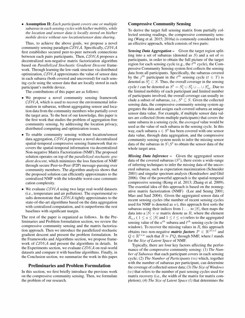
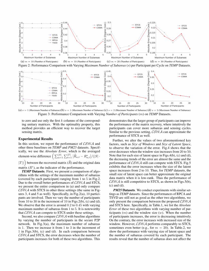
Figure 2: Performance Comparison with Varying Maximum Number of Subareas (s) per Participant per Cycle on TEMP Datasets.

10 3015 20 25 Number of Participants

0

1

2

3

4

5

6

Abs

olut

e E

rror

(D

egre

e C

ent.)

STCSCSWARPCATSVD

(a) s = 1 (Maximum Number of Subareas)

10 3015 20 25 Number of Participants

0.1

0.2

0.3

0.4

0.5

Abs

olut

e E

rror

(D

egre

e C

ent.)

STCSCSWA

(b) s = 1 (Maximum Number of Subareas)

10 3015 20 25 Number of Participants

0.15

0.2

0.25

0.3

0.35

0.4

0.45

Abs

olut

e E

rror

(D

egre

e C

ent.)

STCSCSWA

(c) s = 2 (Maximum Number of Subareas)

10 3015 20 25 Number of Participants

0.15

0.2

0.25

0.3

0.35

0.4

Abs

olut

e E

rror

(D

egre

e C

ent.)

STCSCSWA

(d) s = 3 (Maximum Number of Subareas)

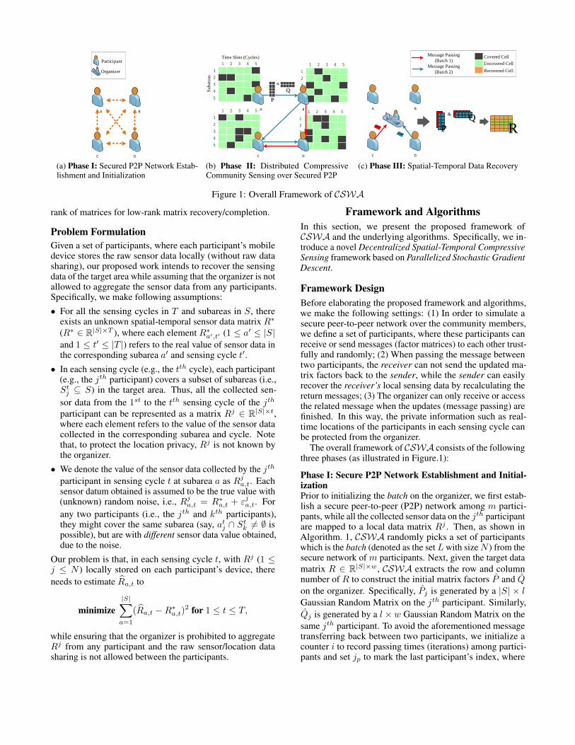
Figure 3: Performance Comparison with Varying Number of Participants (m) on TEMP Datasets.

to zero and use only the first k columns of the correspond-ing unitary matrices. With the optimality property, thismethod provides an efficient way to recover the targetsensing matrix.

Experimental ResultsIn this section, we report the performance of CSWA andother three baselines on TEMP and PM25 datasets. Specif-ically, we use the Absolute Error, which is the averagedelement-wise difference

(∑|S|a=1

∑|T |t=1

∣∣R̂a,t −R∗a,t∣∣/(|S| ·

|T |))

between the recovered matrix (R̂) and the original datamatrix (R∗), as the indicator of the performance.

TEMP Datasets. First, we present a comparison of algo-rithms with the settings of the maximum number of subareas(covered by each participant) ranging from 1 to 5 in Fig.2.Due to the overall better performances of CSWA and STCS,we present the entire comparison in (a) and only compareCSWA with STCS in other three settings (the same in Fig-ures 3, 4 and 5 as well). Specifically, in Fig.2(a), 10 partici-pants are involved. Then we vary the number of participantsfrom 10 to 30 in the increment of 10 in Figs.2(b), (c) and (d).We observe that the error is around 0.2 to 0.45 with varyingmaximum number of subareas from 1 to 5. It is noteworthythat CSWA can compete to STCS under these settings.

Second, we also compare CSWAwith baseline algorithmsby varying the number of participants in the secure P2Pnetwork. In Fig.3(a), the maximum number of subareasis 1. Then we increase it from 1 to 3 in the increment of1 in Figs.3(b), (c) and (d). In each comparison betweenCSWA and STCS, the error decreases when the number ofparticipants increases for both of these two algorithms. This

demonstrates that the larger group of participants can improvethe performance of the matrix recovery, where intuitively theparticipants can cover more subareas and sensing cycles.Similar to the previous setting, CSWA can approximate theperformance of STCS as well.

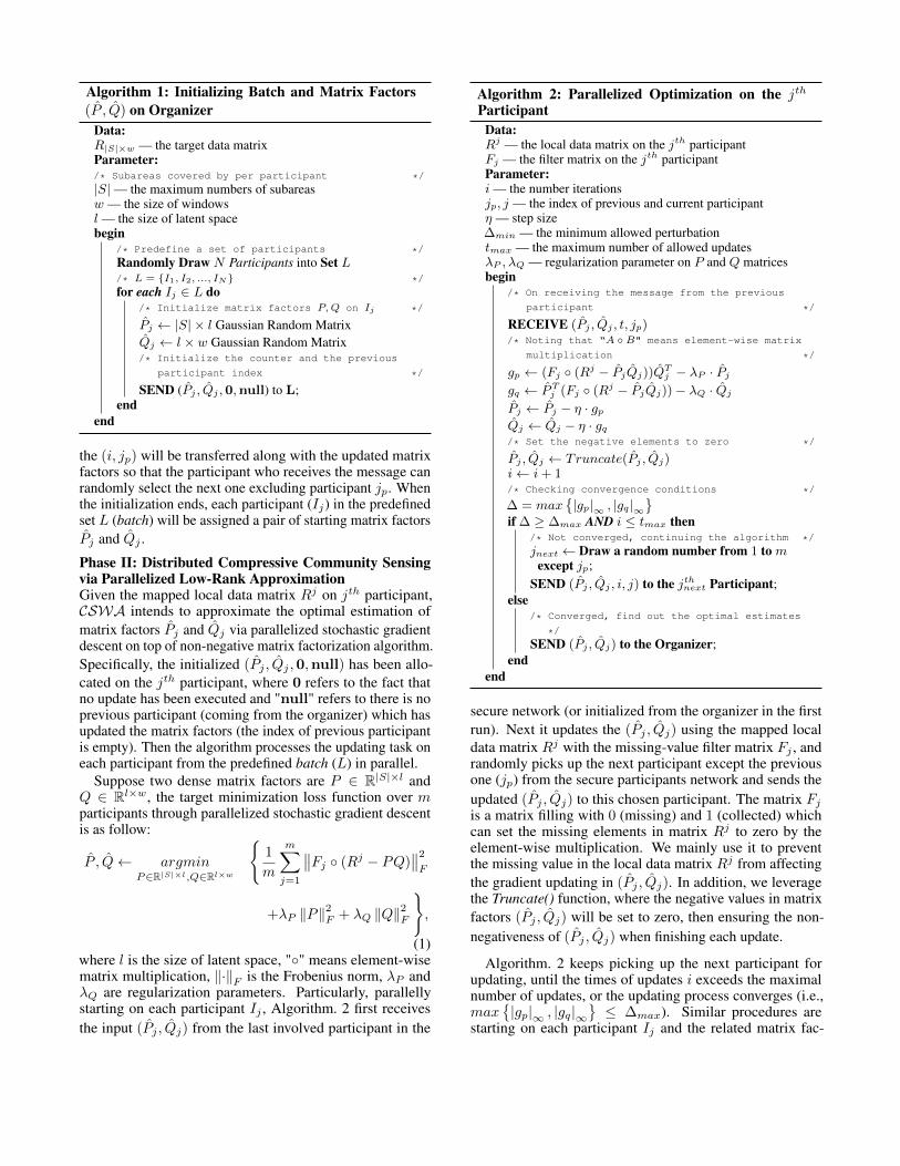
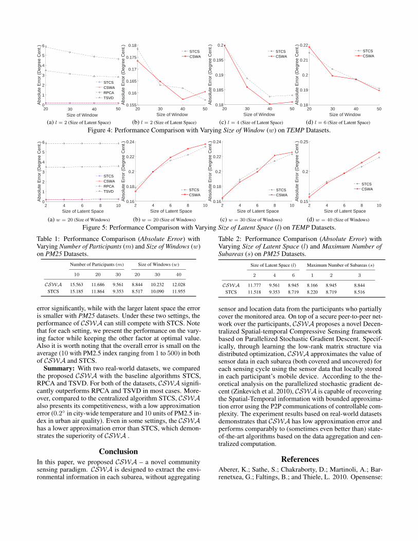
Further, we alter the values of two aforementioned keyfactors, such as Size of Windows and Size of Latent Space,to observe the variation of the error. Fig.4 shows that theerror decreases when the window size increases from 20 to 50.Note that for each size of latent space in Figs.4(b), (c) and (d),the decreasing trends of the error are almost the same and theperformance of CSWA still can compete with STCS. Fig.5exhibits that the error increases when the size of the latentspace increases from 2 to 10. Thus, for TEMP datasets, thesmall size of latent space can better approximate the originaldata matrix when it is low-rank. Thus the performance ofCSWA is still competitive to STCS, as shown in Figs.5(b),(c) and (d).

PM25 Datasets. We conduct experiments with similar set-tings as TEMP datasets. Since the performances of RPCA andTSVD are still not as good as the other two algorithms, weonly present the comparison between the proposed CSWAand STCS here. Specifically, in Table.1, we list the AbsoluteError of these two algorithms with varying number of par-ticipants (m) and the window size (w). When the numberof participants increases, the error is decreasing intuitively.On the contrary, the error increases with increased size of thewindow. However, CSWA performs comparably to STCS,sometimes even better (e.g., for m = 20). In Table.2, weshow the performance with varying size of latent space andthe number of subareas covered by each participant. Theresults reveal that the number of subareas does not affect the

20 5030 40 Size of Window

0

1

2

3

4

5

6

Abs

olut

e E

rror

(D

egre

e C

ent.)

STCSCSWARPCATSVD

(a) l = 2 (Size of Latent Space)

20 5030 40 Size of Window

0.155

0.16

0.165

0.17

0.175

0.18

Abs

olut

e E

rror

(D

egre

e C

ent.)

STCSCSWA

(b) l = 2 (Size of Latent Space)

20 5030 40 Size of Window

0.18

0.185

0.19

0.195

0.2

Abs

olut

e E

rror

(D

egre

e C

ent.)

STCSCSWA

(c) l = 4 (Size of Latent Space)

20 5030 40 Size of Window

0.18

0.19

0.2

0.21

0.22

Abs

olut

e E

rror

(D

egre

e C

ent.)

STCSCSWA

(d) l = 6 (Size of Latent Space)

Figure 4: Performance Comparison with Varying Size of Window (w) on TEMP Datasets.

2 104 6 8 Size of Latent Space

0

1

2

3

4

5

6

Abs

olut

e E

rror

(D

egre

e C

ent.)

STCSCSWARPCATSVD

(a) w = 20 (Size of Windows)

2 104 6 8 Size of Latent Space

0.16

0.18

0.2

0.22

0.24

Abs

olut

e E

rror

(D

egre

e C

ent.)

STCSCSWA

(b) w = 20 (Size of Windows)

2 104 6 8 Size of Latent Space

0.16

0.18

0.2

0.22

0.24

Abs

olut

e E

rror

(D

egre

e C

ent.)

STCSCSWA

(c) w = 30 (Size of Windows)

2 104 6 8 Size of Latent Space

0.15

0.2

0.25

Abs

olut

e E

rror

(D

egre

e C

ent.)

STCSCSWA

(d) w = 40 (Size of Windows)

Figure 5: Performance Comparison with Varying Size of Latent Space (l) on TEMP Datasets.

Table 1: Performance Comparison (Absolute Error) withVarying Number of Participants (m) and Size of Windows (w)on PM25 Datasets.

Number of Participants (m) Size of Windows (w)

10 20 30 20 30 40

CSWA 15.563 11.686 9.561 8.844 10.232 12.028STCS 15.185 11.864 9.353 8.517 10.090 11.955

error significantly, while with the larger latent space the erroris smaller with PM25 datasets. Under these two settings, theperformance of CSWA can still compete with STCS. Notethat for each setting, we present the performance on the vary-ing factor while keeping the other factor at optimal value.Also it is worth noting that the overall error is small on theaverage (10 with PM2.5 index ranging from 1 to 500) in bothof CSWA and STCS.

Summary: With two real-world datasets, we comparedthe proposed CSWA with the baseline algorithms STCS,RPCA and TSVD. For both of the datasets, CSWA signifi-cantly outperforms RPCA and TSVD in most cases. More-over, compared to the centralized algorithm STCS, CSWAalso presents its competitiveness, with a low approximationerror (0.2◦ in city-wide temperature and 10 units of PM2.5 in-dex in urban air quality). Even in some settings, the CSWAhas a lower approximation error than STCS, which demon-strates the superiority of CSWA .

ConclusionIn this paper, we proposed CSWA – a novel communitysensing paradigm. CSWA is designed to extract the envi-ronmental information in each subarea, without aggregating

Table 2: Performance Comparison (Absolute Error) withVarying Size of Latent Space (l) and Maximum Number ofSubareas (s) on PM25 Datasets.

Size of Latent Space (l) Maximum Number of Subareas (s)

2 4 6 1 2 3

CSWA 11.777 9.561 8.945 8.166 8.945 8.844STCS 11.518 9.353 8.719 8.220 8.719 8.516

sensor and location data from the participants who partiallycover the monitored area. On top of a secure peer-to-peer net-work over the participants, CSWA proposes a novel Decen-tralized Spatial-temporal Compressive Sensing frameworkbased on Parallelized Stochastic Gradient Descent. Specif-ically, through learning the low-rank matrix structure viadistributed optimization, CSWA approximates the value ofsensor data in each subarea (both covered and uncovered) foreach sensing cycle using the sensor data that locally storedin each participant’s mobile device. According to the the-oretical analysis on the parallelized stochastic gradient de-cent (Zinkevich et al. 2010), CSWA is capable of recoveringthe Spatial-Temporal information with bounded approxima-tion error using the P2P communications of controllable com-plexity. The experiment results based on real-world datasetsdemonstrates that CSWA has low approximation error andperforms comparably to (sometimes even better than) state-of-the-art algorithms based on the data aggregation and cen-tralized computation.

ReferencesAberer, K.; Sathe, S.; Chakraborty, D.; Martinoli, A.; Bar-renetxea, G.; Faltings, B.; and Thiele, L. 2010. Opensense:

open community driven sensing of environment. In Proceed-ings of the ACM SIGSPATIAL International Workshop onGeoStreaming, 39–42. ACM.Fischler, M. A., and Bolles, R. C. 1981. Random sampleconsensus: a paradigm for model fitting with applications toimage analysis and automated cartography. Communicationsof the ACM 24(6):381–395.Gao, H.; Cai, J.-F.; Shen, Z.; and Zhao, H. 2011. Robust prin-cipal component analysis-based four-dimensional computedtomography. Physics in medicine and biology 56(11):3181.Hachem, S.; Pathak, A.; and Issarny, V. 2013. Probabilisticregistration for large-scale mobile participatory sensing. InPervasive Computing and Communications (PerCom), 2013IEEE International Conference on, 132–140. IEEE.Herring, R.; Hofleitner, A.; Amin, S.; Nasr, T.; Khalek, A.;Abbeel, P.; and Bayen, A. 2010. Using mobile phones toforecast arterial traffic through statistical learning. In 89thTransportation Research Board Annual Meeting, 10–14.Ingelrest, F.; Barrenetxea, G.; Schaefer, G.; Vetterli, M.;Couach, O.; and Parlange, M. 2010. Sensorscope:Application-specific sensor network for environmental mon-itoring. ACM Transactions on Sensor Networks (TOSN)6(2):17.Isam, S.; Kanaras, I.; and Darwazeh, I. 2011. A truncatedsvd approach for fixed complexity spectrally efficient fdmreceivers. In Wireless Communications and Networking Con-ference (WCNC), 2011 IEEE, 1584–1589. IEEE.Ji, S.; Zheng, Y.; and Li, T. 2016. Urban sensing based on hu-man mobility. In Proceedings of the 2016 ACM InternationalJoint Conference on Pervasive and Ubiquitous Computing,1040–1051. ACM.Kondrashov, D., and Ghil, M. 2006. Spatio-temporal fill-ing of missing points in geophysical data sets. NonlinearProcesses in Geophysics 13(2):151–159.Kong, L.; Xia, M.; Liu, X.-Y.; Wu, M.-Y.; and Liu, X. 2013.Data loss and reconstruction in sensor networks. In INFO-COM, 2013 Proceedings IEEE, 1654–1662. IEEE.Lee, D. D., and Seung, H. S. 2001. Algorithms for non-negative matrix factorization. In Advances in neural informa-tion processing systems, 556–562.Liu, T.; Zheng, Y.; Liu, L.; Liu, Y.; and Zhu, Y. 2014.Methods for sensing urban noises. Tec. Rep. MSR-TR-2014-66.Mao, Y., and Saul, L. K. 2004. Modeling distances in large-scale networks by matrix factorization. In Proceedings of the4th ACM SIGCOMM conference on Internet measurement,278–287. ACM.Pan, B.; Zheng, Y.; Wilkie, D.; and Shahabi, C. 2013. Crowdsensing of traffic anomalies based on human mobility andsocial media. In Proceedings of the 21st ACM SIGSPATIALInternational Conference on Advances in Geographic Infor-mation Systems, 344–353. ACM.Schneider, T. 2001. Analysis of incomplete climate data:Estimation of mean values and covariance matrices and impu-tation of missing values. Journal of Climate 14(5):853–871.

Sheng, X.; Tang, J.; and Zhang, W. 2012. Energy-efficientcollaborative sensing with mobile phones. In INFOCOM,2012 Proceedings IEEE, 1916–1924. IEEE.Wang, L.; Zhang, D.; Pathak, A.; Chen, C.; Xiong, H.; Yang,D.; and Wang, Y. 2015. Ccs-ta: Quality-guaranteed onlinetask allocation in compressive crowdsensing. In Proceedingsof the 2015 ACM International Joint Conference on Pervasiveand Ubiquitous Computing, 683–694. ACM.Wang, L.; Zhang, D.; Wang, Y.; Chen, C.; Han, X.; andM’hamed, A. 2016a. Sparse mobile crowdsensing: chal-lenges and opportunities. IEEE Communications Magazine54(7):161–167.Wang, L.; Zhang, D.; Yang, D.; Lim, B. Y.; and Ma, X. 2016b.Differential location privacy for sparse mobile crowdsens-ing. In Data Mining (ICDM), 2016 IEEE 16th InternationalConference on, 1257–1262. IEEE.Wang, L.; Yang, D.; Han, X.; Wang, T.; Zhang, D.; and Ma,X. 2017a. Location privacy-preserving task allocation formobile crowdsensing with differential geo-obfuscation. InProceedings of the 26th International Conference on WorldWide Web, 627–636. International World Wide Web Confer-ences Steering Committee.Wang, L.; Zhang, D.; Wang, P.; Animesh, C.; Han, X.; andXiong, W. 2017b. Space-ta: Cost-effective task alloca-tion exploiting intra- and inter-data correlations in sparsecrowdsensing. ACM Transactions on Intelligent Systems andTechnology.Xiong, H.; Zhang, D.; Wang, L.; and Chaouchi, H. 2015.Emc 3: Energy-efficient data transfer in mobile crowdsensingunder full coverage constraint. IEEE Transactions on MobileComputing 14(7):1355–1368.Yoon, J.; Noble, B.; and Liu, M. 2007. Surface streettraffic estimation. In Proceedings of the 5th internationalconference on Mobile systems, applications and services,220–232. ACM.Zhang, Y.; Roughan, M.; Willinger, W.; and Qiu, L. 2009.Spatio-temporal compressive sensing and internet traffic ma-trices. In ACM SIGCOMM Computer Communication Re-view, volume 39, 267–278. ACM.Zhang, D.; Wang, L.; Xiong, H.; and Guo, B. 2014a. 4w1hin mobile crowd sensing. IEEE Communications Magazine52(8):42–48.Zhang, D.; Xiong, H.; Wang, L.; and Chen, G. 2014b. Crow-drecruiter: selecting participants for piggyback crowdsensingunder probabilistic coverage constraint. In Proceedings ofthe 2014 ACM International Joint Conference on Pervasiveand Ubiquitous Computing, 703–714. ACM.Zheng, Y.; Liu, F.; and Hsieh, H.-P. 2013. U-air: When urbanair quality inference meets big data. In Proceedings of the19th ACM SIGKDD international conference on Knowledgediscovery and data mining, 1436–1444. ACM.Zinkevich, M.; Weimer, M.; Li, L.; and Smola, A. J. 2010.Parallelized stochastic gradient descent. In Advances in neu-ral information processing systems, 2595–2603.