cubature methods and applications

Cubature Methods and Applications

Dan Crisan

Imperial College London

CEMRACS 2017Numerical methods for stochastic models:

control, uncertainty quantification, mean-fieldJuly 17 - August 25

CIRM, Marseille

Dan Crisan (Imperial College London) Particle approximations to PDEs ans SPDEs 18 July 2017 1 / 40

Talk Synopsis

Feynman-Kac representations - a common platformTheoretical Analysis of solution of PDEsApproximation of Feynman-Kac representations

Wiener measure approximationComputational effort

Example 1: Semilinear PDEs (joint work with K. Manolarakis)The Feynman-Kac representationFunctional discretizationTheoretical resultsNumerical Implementation

Example 2: linear parabolic SPDEs (joint work with S. Ortiz-Latorre)The Feynman-Kac representationFunctional discretizationTheoretical resultsNumerical Implementation

Example 3: McKean-Vlasov PDEs (joint work with E. McMurray)The Feynman-Kac representationFunctional discretizationTheoretical resultsNumerical Implementation

Final remarksDan Crisan (Imperial College London) Particle approximations to PDEs ans SPDEs 18 July 2017 2 / 40

Feynman-Kac representations A common platform

Common feature of many PDEs: their solutions can be represented asintegrals of certain nonlinear functionals with respect to the Wiener measure.

Feynman-Kac formula

u(t , x) = E [Λt,x (W )] =

∫ω∈C([0,∞),Rd )

Λt,x (ω)dPW (ω)

Microscopic level Macroscopic level Timeline

Brownian motionW = Wt , t ≥ 0

Heat equation

∂t ut = 1

2 ∆utu0 = Φ

Feynman 1948 Kac 1949

Zakai equation dut = Lut + hut dYt Duncan, Mortensen, Zakai 1970

McKean-Vlasov PDEs∂t ut =

∑di,j=1 aij (ut )∂i∂j ut

+∑d

i=1 bi (ut )∂i ut + c(ut )utGartner 1988

Semilinear PDEs

∂t ut = Lut + f(t, x, ut ,∇ut

)u0 = Φ

Pardoux & Peng 1990, 1992

Fully Nonlinear PDEs F (t, x, ut ,∇ut ,∆ut ) = 0 Soner, Touzi & Victoir 2007

3 − d incompressibleNavier − Stokes equation

∂t ut + (ut · ∇)ut − ν∆ut +∇p = 0

∇ · ut = 0 Constantin & Iyer 2008

K-S equation dut = Lut + ut (h)(dYt − ut (h)dt) Crisan & Xiong 2009

viscous Burgers equation ∂t ut + ut∂x ut − ν∂2x ut = 0 Novikov & Iyer 2010


Feynman-Kac representations Theoretical Analysis of Feynman-Kac formulae

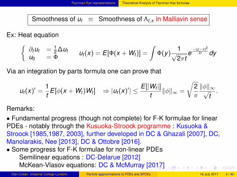
Smoothness of ut ≡ Smoothness of Λt,x in Malliavin sense

Ex: Heat equation∂tut = 1

2 ∆utu0 = Φ

ut (x) = E [Φ(x + Wt )] =

∫Φ(y)

1√2πt

e−(y−x)2

2t dy

Via an integration by parts formula one can prove that

ut (x)′ =1t

E [φ(x + Wt )Wt ] ⇒ |ut (x)′| ≤ E [|Wt |]t‖φ‖∞ =

√2π

‖φ‖∞√t.

Remarks:• Fundamental progress (though not complete) for F-K formulae for linearPDEs - notably through the Kusuoka-Stroock programme : Kusuoka &Stroock [1985,1987, 2003], further developed in DC & Ghazali [2007], DC,Manolarakis, Nee [2013], DC & Ottobre [2016].• Some progress for F-K formulae for non-linear PDEs

Semilinear equations : DC-Delarue [2012]McKean-Vlasov equations: DC & McMurray [2017]


Feynman-Kac representations Approximation of Feynman-Kac representation

u(t , x) = E [Λt,x (W )] =

∫ω∈C([0,∞),Rd )

Λt,x (ω)dPW (ω)

A three-step scheme:replace PW with PW = 1

n

∑ni=1 δωi - W approximates the signature of W

approximate Λt,x with an explicit/simple version Λt,x

control the computational effort (use the TBBA)

u(t , x) ' 1n

n∑i=1

Λt,x (ωi )

Full DNA Typical Paths Representative Paths Truncated DNA


Feynman-Kac representations Wiener measure approximation

Chen’s iterated integrals expansion - signature of a path

Let T(Rd)

=⊕∞

i=0 (Rd )⊗i

and T (m)(Rd)

=⊕m

i=0(Rd )⊗i be the tensor algebraof all non-commutative polynomials over Rd and, respectively the tensoralgebra of all non-commutative polynomials of degree less than m + 1. For apath ω ∈ Cbv ([0,∞),Rd ) define its signature St (ω) and, respectively, itstruncated signature Sm

t (ω) to be the corresponding Chen’s iterated integralsexpansion:

S : Cbv ([0,∞),Rd )→T(Rd)

St (ω) =∞∑

k=0

∫0<t1...tk<t

dωt1 ⊗ ...⊗ dωtk

Sm : Cbv ([0,∞),Rd )→T (m)(Rd)

Smt (ω) =

m∑k=0

∫0<t1...tk<t

dωt1 ⊗ ...⊗ dωtk .

The (random) signature and, respectively, the truncated signature of theBrownian motion are

St (W ) =∞∑

k=0

∫0<t1...tk<t

dWt1⊗...⊗dWtk , Smt (W ) =

m∑k=0

∫0<t1...tk<t

dWt1⊗...⊗dWtk .



E [St (W )] uniquely identifies the Wiener measure PW .

If W is another process such that E [Smt (W )] = E

[Sm

t (W )], then

E [Λt,x (W )] ' E [Λt,x (W )] high order approximation of u(t , x).

See DC and Ghazali [2007] for conditions.Several choices for W : Kusuoka [2001,2004], Kusuoka and Ninomiya[2004], Lyons and Victoir. [2004], Ninomiya and Victoir [2004], etc.

Theorem (Lyons & Victoir (2004))

For any t > 0, there exists paths ω1, . . . , ωN ∈ C00,bv([0, t ];Rd ) and

λ1, λ2, . . . , λN (∑N

i=1 λi = 1), such that if P(W = ωi ) = λi then

E [Smt (W )] = E

[Sm

t (W )].

If the above is true, we call LW =∑N

i=1 λiδωi the cubature measure anddenote it by Qm

t .



For example, if we want to approximate E[α(Xt )], where X is the the solutionof the following SDE

dXt = V0(Xt )dt +d∑

i=1

Vi (Xt ) dW it

Then X can be expressed as X = Ψt (W ) giving a representation of the formE[Λt (W )]. Choose X j to be the solution of the following ODE

dX jt = V0(X j

t )dt +d∑

i=1

Vi (Xjt )dωj,i

t

In this case:

E[Λt (W )] = EQm [α(Xt )] =N∑

i=1

λig(X jt )

and|E[Λt (W )]− E[Λt (W )]| ≤ Cδ

m−12 .



Cubature of order 3: For d=1, we can use 2 paths with equal weights λj = 12

defined asωj

t = tz i ,

where z i ∈ −1,1. For d ≥ 2 , we can use[

d(d + 2)

6

]+ 1 linear paths with

equal weights λj .

Cubature of order 5: For d=1, we can use 3 paths, ω, −ω and 0 with ω isdefined as

ω(t) =

√

32

(4−√

22)

t t ∈[0, 1

3

]√

36

(4−√

22)

+√

3(−1 +

√22) (

t − 13

)t ∈

[ 13 ,

23

]√

36

(2 +√

22)

+√

32

(4−√

22) (

t − 23

)t ∈

[ 23 ,1]


Feynman-Kac representations Computational effort reduction

• An additional procedure is used to control the computational effort.• The measure Qm is replaced by a measure Qm,N with support of size N byusing a tree based branching algorithm (TBBA).• The TBBA was introduced in DC & Lyons (2002) as the optimal stratifiedsampling procedure in the context of the filtering problem. The method has awider applicability: it is applicable to any method that uses branching trees.• By merging the TBBA with the cubature method we keep the number ofparticles on the support of the intermediate measures constant.


Feynman-Kac representations Computational effort reduction

• Assume that we constructed Qm =∑M

j=1 λjδγj with M paths and we want toreduce the number to at most N paths.•We replace Qm with a random measure Qm,N such that supp(Qm,N) ⊆supp(Qm) and that the size on its support is at most N. For an arbitrary pathγ ∈ supp(Qm), we will have

Qmk (γ) =

bNQm(γ)c

N with probability 1− NQm(γ)bNQm(γ)c+1

N with probability NQm(γ). (1)

• In addition, Qm,N is constructed so that it is a (random) probability measure,i.e., ∑

γ∈suppQm

Qmk (γ) = 1. (2)

• The mass allocated to each path γ ∈ supp(Qm) is either 0 or an integermultiple of 1/N ⇒ the support of any realization of Qm,N has size at most N.• The maximum number of paths is achieved when Qm,N puts mass 1/N on Nof the M paths. This is the basis of the control of the computational effort.


. Example 1: Semilinear PDEs

Let u ∈ C1,2([0,T ]× Rm) be the solution of the final value Cauchy problem(∂t + L)u = −f (t , x ,u,V1u, ...,Vdu) (x)) , t ∈ [0,T ), x ∈ Rm

u(T , x) = Φ(x), x ∈ Rm , (3)

whereL is the second order differential operator

L = V0 +12

d∑i=1

V 2i . (4)

In (4) Vi , i = 0,1...,d are the first differential operators associated toVi = (V j

i )dj=1.

Vi =m∑

j=1

V ji ∂xi

Particular case(∂t + ∆)u = −f (t , x ,u,∇u) (x)) , t ∈ [0,T ), x ∈ Rm

u(T , x) = Φ(x), x ∈ Rm , (5)


. The Feynman-Kac formula ( forward-backward SDEs)

Let (Ω,F ,P) be complete probability space endowed with a filtration thatsatisfies the usual conditions Ftt≥0. Let W be an Ft-adapted Brownianmotion and (X ,Y ,Z ) = (Xt ,Yt ,Zt ), t ∈ [0,T ] be the solution of the(decoupled) system:

Forward-Backward SDE

Xt = X0 +

∫ t

0V0(Xs)ds +

d∑i=1

∫ t

0Vi (Xs) dW i

s, forward c. (6)

Yt = Φ(XT ) +

∫ T

tf (s,Xs,Ys,Zs)ds −

d∑i=1

∫ T

tZ i

sdW is, backward c. (7)

- X m-dimensional, Y 1-dimensional, Z d-dimensional- Vi : Rm → Rm smooth vector fields Vi ∈ C∞b (Rm,Rm), i = 0,1, ...,d- The stochastic integral in (6) is a Stratonovitch type integral- Φ(XT ) called the final condition- f : [0,T ]× Rm × R × Rd → R Lipschitz, called ”the driver”.

Theorem (Pardoux & Peng (1990))

There exists a unique Ft -adapted solution (X ,Y ,Z ) of the system (6)+(7).


. The Feynman-Kac formula ( forward-backward SDEs)

Theorem (Peng 1991,1992, Pardoux & Peng 1992)

Under additional smoothness assumptions on the coefficients of the FBDSE,the unique solution of the Cauchy problem (5) admits the followingFeynman-Kac representation

u(t , x) = Y t,xt = E

[Φ(X t,x (T )) +

∫ T

tf (s,X t,x

s ,Y t,xs ,Z t,x

s )ds

], (8)

where (X t,x ,Y t,x ,Z t,x ) is the ‘stochastic flow’ associated FBSDE (6)+(7)

X t,xs = x +

∫ s

tV0(X t,x

u )du +d∑

i=1

∫ s

tVi (X

t,xu ) dW i

u, s ∈ [t ,T ], (9)

Y t,xs = Φ(X t,x

T ) +

∫ T

sf (u,X t,x

u ,Y t,xu ,Z t,x

u )du −d∑

i=1

∫ T

s(Z t,x

u )idW iu. (10)

Moreover (Z t,xs )i = Viu(s,X t,x

s ) for s ∈ [t ,T ].


. Functional discretization

We deduce from the Feynman-Kac representation (8) and the formula for Zthat:

u(t , x) = E

[Φ(XT ) +

∫ T

tf (s,Xs,u(s,Xs), (V1u, . . . ,Vdu)(s,Xs))ds

]

Hence there exists Λt : CRd [t ,T ]→ R such that

u(t , x) = E[Λt

(X t,x

[t,T ]

)].

Let π := 0 = t0 < t1 < . . . < tn = T be a partition of [0,T ], with δ = ti+1 − ti ,∆Wi+1 = Wti+1 −Wti .Define Rng = g and Sng = ∇gV or Sng = 0 if g not Lipschitz.For i = 0, . . . ,n − 1, we define the operators R i , Si :

Rig(x) = E[Ri+1g(X ti ,x

ti+1)]

+ δf (ti , x ,Rig(x),Sig(x))

Sig(x) =1δE[Ri+1g(X ti ,x

ti+1)∆Wi+1

]



Let:uδ(0, x) = E

[Λ(Xt0 ,Xt1 , ...,Xtn )

]= R0Φ(x).

Theorem (Bouchard & Touzi 2004, Gobet & Labart 2007, DC & Manolarakis2010)

For f Lipschitzsup

x∈Rd|uδ(0, x)− u(0, x)| ≤ C

√δ.

For f smoothsup

x∈Rd|uδ(0, x)− u(0, x)| ≤ Cδ.

Other discretizations methods are possible: Zhang 2005, DC & Manolarakis2010, Chassagneux & DC 2013



Next we use the cubature measure Qm of degree m = 3,5,7, ... coupled withthe TBBA procedure to produce a measure Qm,N with support of size N . Forevery i = 0, . . . ,n − 1 define the operators R i , Si

Rig(x) = EQm,N

[Ri+1g(X ti ,x

ti+1)]

+ δf (ti , x , Rig(x), Sig(x))

Sig(x) =1δEQm,N

[Ri+1g(X ti ,x

ti+1)∆Wi+1

]Let uδ(0, x) = EQm,N

[Λ(Xt0 ,Xt1 , ...,Xtn )

]= R0Φ(x).

Theorem (D.C. & Manolarakis, 2011)

supx∈Rd

E[|uδ(0, x)− u(0, x)|2] ≤ C(δ + δ

m−12 +

1N

).


. Numerical Implementation

Let u ∈ C1,2([0,T ]× R4) be the solution of the final value Cauchy problem(∂t + L)u = −f (t , x ,u,∆u)) , t ∈ [0,T ), x ∈ R4

u(T , x) = Φ(x), x ∈ R,

where

Lϕ(x) =4∑

i=1

µixidϕdxi

+σ2

i x2i

2d2ϕ

dx2i

x ∈ R.

f (t , x , y , z) = −ry −∑4

i=1(µi − r)zi , x ∈ R.Φ(x) = (x1x2x3x4 − k)+.



The randomness can be reduced by averaging over independent copies


. Example 2: Linear SPDEs with multiplicative noise

(Ω,F ,P) probability space,W m-dimensional standard Brownian motionρ = ρt , t ≥ 0 MF

(Rd)-valued stochastic process.

dρt (ϕ) = ρt (Aϕ)dt +m∑

k=1

ρt (γkϕ)dW kt . (11)

where

Aϕ (x) =12

d∑i,j=1

aij (x) ∂i∂jϕ (x) +d∑

i=1

bi (x) ∂iϕ (x)

a = σσ>

Particular case:

dρt (z) = ∆ρt (z)dt +m∑

k=1

γkρt (z)dW kt .


. The filtering problem

(Ω,F , P) probability spaceV = (V i

t )pi=1, t ≥ 0, U =

(U i

t)m

i=1 , t ≥ 0 independent Brownian motions

Xt = X0 +

∫ t

0b (Xs) ds +

∫ t

0σ (Xs) dVs

Wt =

∫ t

0γ (Xs) ds + Ut ,

The filtering problem: Find the conditional law of the signal Xt givenWt = σ(Ws, s ∈ [0, t ]), i.e.,

ϑt (ϕ) = E[ϕ(Xt )|Wt ], t ≥ 0, ϕ ∈B(Rd ).

Theorem

ϑt =ρt

ρt (1),

where ρt (1) =

∫Rd

1ρt (dx) = ρt (Rd ).


. The Feynman-Kac formula

The process W becomes a Brownian motion via a change of measure(Girsanov’s theorem)

dPdP

∣∣∣∣Ft

= Zt4= exp

(−∫ t

0

m∑k=1

γk (Xs) dUks −

12

∫ t

0

m∑k=1

γk (Xs)2 ds

), t ≥ 0.

Under P, W is a Brownian motion and X satisfies:

Xt = X0 +

∫ t

0b (Xs) ds +

∫ t

0σ (Xs) dVs.

The Feynman-Kac formula

ρt (ϕ) = E

[ϕ(Xt ) exp

(∫ t

0

m∑k=1

γk (Xs) dW ks −

12

∫ t

0

m∑k=1

γk (Xs)2 ds

)∣∣∣∣∣Wt

](12)

ρt (ϕ) is the expected value of a functional of X which depends Wto approximate numerically ρt (ϕ) we need to

approximate the functional with a simpler versionapproximate the law of the process Xcontrol the computational effort



Consider the equidistant partition itn

ni=0 and let gi be the noise dependent

functions

gi =m∑

j=1

(γ j (W jitn−W j

(i−1)tn

)− t2n

(γ j )2).

Define the operators

Rnsϕ (x) = E[ϕ(Xs(x))]

R isϕ (x) = E[ϕ(Xs(x)) exp (gi ( Xs(x)))|Wt ]

for i = 0, ..,n − 1. Let ρnt be the approximate measure

ρnt (ϕ) = E [ϕ(Xt )Z n

t (X ,W )|Wt ] = E[

R0tnR1

tn...Rn

tnϕ (X0)

∣∣∣Wt

]Z n

t (X ,W ) =n∏

i=1

exp

(m∑

k=1

(γk (Xs) (W it

n−W (i−1)t

n)− t

2nγk (Xs)2

))

Finally define ϑnt (ϕ) by the formula ϑn

t (ϕ) =ρn

t (ϕ)

ρnt (1)

.



M. All moments of X0 are finite. The functions b, σ are Lipschitz.FLp. E [Zt (X ,W )p] <∞ and supn E [Z n

t (X ,W )p] <∞ for some p > 2.

Condition FLp holds true if γ is bounded. If γ is unbounded, but it has lineargrowth, then the condition is satisfied if X has exponential moments uniformlybounded on [0, t ].

Theorem

Assume that conditions M and FLp hold true and γk , k = 1, ...,m areLipschitz. Then, if ϕ has polynomial growth, there exists a constantc = c (ϕ, t) independent of n such that

E[|ρn

t ϕ− ρtϕ|2]≤ c

n.

Moreover, if supn E[(ϑnt (ϕ))2] <∞, then

E [|ϑnt ϕ− ϑtϕ|] ≤

c√n,

where, again, c = c (ϕ, t) is a constant independent of n.



AP. Let (Ps)s≥0 be the semigroup associated to the Markov process X . Wewill assume that, for any Lipschitz continuous function ψ : Rd→ R, Psψ istwice differentiable for any s ∈ [0, t ]. Moreover, if

Pa,bψ , Paψ − Pbψ,a,b ∈ [0, t ] ,

we will assume that there exists a constant c7 = c7 (t) independent of a and bsuch that

supx∈Rd

|Pa,bψ (x)| ≤ ckψ(√

a−√

b)

(13)

supx∈Rd

|∂iPa,bψ| ≤cb

kψ (a− b) , i = 1, ...,d , (14)

where kψ is the Lipschitz constant of ψ.

Inequalities (13) and (14) are satisfied if, for example, f , σ =(σi)d

i=1 ∈ C∞b (Rd )

and the vector fields(σi)d

i=1 satisfy the Hormander condition.



Theorem

Assume that conditions M, FLp and AP hold true. Assume also that thefunctions ϕ and γi i = 1, ..,m are Lipschitz. Then there exists N > 0 such thatfor all n > N and ε ∈ (0,1), there exists a constant c = c (ϕ, t ,N, ε)independent of the partition such that

E[|ρn


n2−ε .

Moreover, if supn E[(ϑnt (ϕ))2] <∞, then for all n > N and ε ∈ (0,1), there

exists a constant c = c (ϕ, t ,N, ε) independent of the partition such that


cn1−ε .



TheoremAssume that conditions M, FLp are satisfied and that the functionsγi ∈ C2

b (Rd ) for i = 1, ..,m. Then, if ϕ has polynomial growth, there exists aconstant c = c (ϕ, t) independent of n such that

E[|ρn


n2 . (15)

Moreover, if supn E[(ϑnt (ϕ))2] <∞,


cn,

where, again, c = c (ϕ, t) is a constant independent of n.


. Approximation of the law of X

Introduce the operators

Rnsϕ (x) = EQm [ϕ(X x

s )]

R isϕ (x) = EQm [ϕ(X x

s ) exp (gi ( X xs ))]

Recall that ρnt (ϕ) = E

[R0

tnR1

tn...Rn

tnϕ (X0)

∣∣∣Wt

]with corresponding

approximationρn

t (ϕ) = EQm

[R0

tnR1

tn...Rn

tnϕ (X0)

∣∣∣Wt

].

Theorem

For all ϕ ∈ Cm+2b (Rd ) and p ≥ 1,

||ρnt (ϕ)− ρn

t (ϕ)||p ≤c

n(m−1)/2

m+2∑i=1

||∇iϕ||∞.

where c = c(t ,m,p) is independent of n.


. Controlling the computational effort

A third procedure is used to control the computational effort. The measure Qm

is replaced by a measure Qm,N with support of size N by using a tree basedbranching algorithm (TBBA). Recall that

Rnsϕ (x) = EQm,N [ϕ(X x

s )], R isϕ (x) = EQm,N [ϕ(X x

s ) exp (gi ( X xs ))],

ρnt (ϕ) = EQm,N

[R0

tnR1

tn...Rn

tnϕ (X0)

∣∣∣Wt

]Theorem

E[|ρnt (ϕ)− ρn

t (ϕ) |2] ≤ CN.

Corollary

E[|ρnt (ϕ)− ρt (ϕ) |2] ≤ C

(1

nα+

1

nm−1

2

+1N

).



Consider the 1-dimensional model:

dρt (ϕ) = ρt (Aϕ)dt + ρt (γϕ)dWt .

where

Aϕ(x) =σ2

2d2ϕ

dx2 (x) + µσ tanh(µxσ

) dϕdx

(x)

γ(x) = h1x + h2

Then

ρt ' w+N (A+t /(2Bt ),1/(2Bt )) + w−N (A−t /(2Bt ),1/(2Bt )),

where

w±t , exp((A±t )2/(4Bt )

)/(exp

((A+

t )2/(4Bt ))

+ exp((A−t )2/(4Bt )

))

A±t , ±µσ

+ h1Ψt +h2 + h1x0

σ sinh (h1σt)− h2

σcoth (h1σt) ,

Bt ,h1

2σcoth (h1σt) ,

Ψt ,∫ t

0

sinh(h1σs)

sinh(h1σt)dWs,


. McKean-Vlasov SDEs

Consider

∂tut (x) =d∑

i=1

V i (x ,ut (ϕi )))2ut (x) + V 0(x ,ut (ϕ0)))ut (x), ut = f

Thenu(0, x) = E [f (X x

T )] ,

where X is a solution of a McKean-Vlasov SDE with smooth scalar interaction

X xt = x +

∫ t

0V0(X x

s ,E[ϕ0(X xs )]) ds +

d∑i=1

∫ t

0Vi (X x

s ,E[ϕi (X xs )]) dBi

s, (16)

scalar interaction := the dependence on the solution through integralsagainst scalar functions,

E[ϕ0(X xs )], E[ϕi (X x

s )], i = 1, ...,d .

ϕi ∈ C∞b (RN ;R), Vi ∈ C∞b (RN+1;RN).

B =(B1, . . . ,Bd

)d-dim standard Brownian motion.

The process X gives a probabilistic representation of a nonlinear PDE.


. Main Assumptions

V0, . . . ,Vd : RN ×R→ RN are vector fields Vi (·, x ′) on RN parametrised by thesecond variable, x ′ ∈ R, with the Lie Bracket between any two given by

[Vi ,Vj ](x , x ′) = ∂xVj (x , x ′)Vi (x , x ′)− ∂xVi (x , x ′)Vj (x , x ′),

where ∂Vi (x , x ′) := (∂xl Vki (x , x ′))1≤k,l≤N is the Jacobian matrix of Vi and

similarly for ∂xVj . Then, for α ∈⋃

k≥11, . . . ,Nk and i ∈ 1, . . . ,N, we defineinductively

V[i] := Vi , V[α∗i] := [Vi ,V[α]] .

(A1): Uniform strong Hormander condition: There exist δ > 0 and m ∈ N suchthat for all ξ ∈ RN ,

inf(x,x′)∈RN×R

∑α∈∪m

k=11,...,Nk

〈V[α](x , x ′), ξ〉2 ≥ δ |ξ|2

(A2): Smoothness of coefficients:

ϕi ∈ C∞b (RN ;R), Vi ∈ C∞b (RN × R;RN) i = 0, . . . ,d


. Main Assumptions

Two algorithms

Partition [0,T ] into 0 = t0 < t1 < . . . < tn = T

X xt = x +

∫ t

0V0(X x

s ,E[ϕ0(X xs )]) ds +

d∑i=1

∫ t

0Vi (X x

s ,E[ϕi (X xs )]) dBi

s,

Taylor method TM

• Introduced by Chaudru de Raynal & Garcia-Trillos [2015].• Over the interval [tj , tj+1] replace Eϕi (X x

t ) appearing in the coefficients withthe cubature approximation of the Taylor expansion of the path t 7→ Eϕi (X x

t )around tj up to some order, q.

Lagrange interpolation method LIM

• Over the interval [tj , tj+1] replace Eϕi (X xt ) with a Lagrange polynomial which

interpolates the cubature approximation of Eϕi (X xt ) at the previous r points in

the time partition.


. Main Assumptions

E(T , x , l ,Πn) - the global error. Parameters:

• r the maximal no of interpolation points required to approximate Eϕi (X0,yt )

• q the truncation of the Taylor expansion of Eϕi (X0,yt )

• n no. of partition points.• l the cubature order.

Theorem (DC, McMurray, 2016)

Let f ∈ C∞b (RN ;R). Then, the error for the Taylor method satisfies

supx∈RN

|E(T , x , l ,Πn)| ≤ Cn−1∑j=0

(tj+1 − tj )A(q,l),

where A(q, l) := (q + 2) ∧ (l + 1)/2. The error in the Lagrange interpolationmethod is

supx∈RN

|E(T , x , l ,Πn)| ≤ Cn−1∑j=0

(tj+1 − tj )

((j + 1) ∧ r)!

j∧(r−1)∏k=0

(tj+1−tj−k )+(tj+1−tj )(l+1)/2.


. Main Assumptions

Parameters:

• γ controls the choice of the Kusuoka partition Πγn• m level required for the uniform strong Hormander condition

Theorem (DC, McMurray, 2016)

Suppose f is only Lipschitz continuous. Assuming that we use the Kusuokapartition Πγn with γ > l − 1, then the error in the TM satisfies

m = 1 : supx∈RN

|E(T , x , l ,Πγn )| ≤ C n−B(q,l)−1/2, (17)

m ≥ 2 : supx∈RN

|E(T , x , l ,Πγn )| ≤ C n−B(q,l), (18)

where B(q, l) = (q + 12 ) ∧ l−2

2 . Assuming that we use the modified Kusuokapartition Πγ,rn with γ ∈ (l − 1, l), then the error in the LIM satisfies

m = 1 : supx∈RN

∣∣E(T , x , l ,Πγ,rn )∣∣ ≤ C n−D(r ,l)−1/2 (1− r/n)−l/2, (19)

m ≥ 2 : supx∈RN

∣∣E(T , x , l ,Πγ,rn )∣∣ ≤ C n−D(r ,l) (1− r/n)−l/2, (20)

where D(r , l) = (r − 32 ) ∧ l−2

2 .


. Numerical Examples

Example 1

N = d = 1:

X 0,xt = x +

∫ t

0E[X 0,x

s

]ds + Bt , X x

t = xet + Bt , EX 0,xt = xet

Terminal function f (x) = x+ := maxx ,0 and, by integrating the Gaussiandensity, we can compute

E(X 0,xt )+ =

√tφ(

xet√

t

)+ xet

(1− Φ

(−xet√

t

)),

where φ and Φ are the density and cumulative distribution function,respectively, of a standard Gaussian random variable.

• The Taylor approximation of order q is easy to compute:T q

t

(EX 0,x

t

)=∑q

k=0xk! tk .

• Cubature formula of degree 5• A fourth order adaptive Runge-Kutta scheme to solve the ODEs.• To achieve order 2 convergence with a cubature formula of degree 5choose q ≥ 1 and γ ∈ (4,5) with Taylor method and r ≥ 3 in the Lagrangeinterpolation method.



• Parameters (x ,T , γ, q, r) = (0.5,10,4.5,2,3).

0 0.2 0.4 0.6 0.8 1 1.2

log10(n)-4

-3.5

-3

-2.5

-2

-1.5

-1

-0.5

0

log10(relativeerror) Lagrange

Gradient = -2.22TaylorGradient = -2.8

Figure: log-log error plot comparison between the LIM and TM. The gradient of eachsolid line is given by a linear regression on the last 5 points.

• Both methods achieve the expected quadratic convergence rate.• TM performs better than LIM.



Example 2

• coefficients are not uniformly elliptic and N = d = 2.• X 0,x

t =(X 1

t ,X2t)

(X 1

tX 2

t

)=

(x1x2

)+

∫ t

0

([2 + sin

(EX 2

s)]

X 1t

) dB1

s +

∫ t

0

(X 2

tX 1

t

) dB2

s ,

where the coefficients are

V0 ≡ 0, V1(x1, x2, x ′) =

(2 + sin(x ′)

x1

), V2(x1, x2, x ′) =

(x2x1

), ϕ1(x1, x2) = x2,

for all (x1, x2, x ′) ∈ R3.• At x1 = 0 the coefficients degenerate.•

V[(1,2)](x1, x2, x ′) =

(x1

2 + sin(x ′)− x1

).

• Since x1 and 2 + sin(x ′)− x1 cannot both be zero at the same time, we seethat V1,V2 and V[(1,2)] span R2. The coefficients satisfy the uniform strongHormander condition, for m = 2.



• For m = 2, with a cubature formula of degree 5 (NCub = 13), we expect toachieve a convergence rate of 3/2. To do so, we have to choose γ ∈ (4,5)and r > 7/2.• Parameters (x1, x2,T , γ, r) = (1,0.5,1,4.5,4) and f (x) = x+.• No explicit solution, we compare the cubature approximation to a MonteCarlo approximation with Euler-Maruyama discretisation.

0 0.2 0.4 0.6 0.8 1 1.2

log10(n)-3.5

-3

-2.5

-2

-1.5

-1

-0.5

log10(relativeerror) Lagrange

Gradient = -2.05TaylorGradient = -1.97

Figure: The gradient of each line is given by a linear regression on the last 5 points.

The performance of the algorithms is similar. Empirically we observe secondorder convergence, whereas a rate of 3/2 is predicted.


. Final remarks

The solution of a variety of deterministic and stochastic PDEs can beanalyzed and/or approximated through their corresponding Feynman-Kacrepresentations.The common methodology contains three steps: functional discretization,Wiener measure approximation (cubature method) and computationaleffort reduction (TBBA).The cubature method is essentially deterministic. The diffusionapproximation uses a set of ordinary differential equations to approximatethe distribution of the solution of the SDE.The (exponentially) increase in the computational effort is controlled bythe TBBA (a random method).A first step towards a unified theory of approximations


cubature methods and applications

Documents