4th International Conference on Earthquake Engineering Taipei, Taiwan

October 12-13, 2006

Paper No. 5

CUBOIDAL INFINITE ELEMENTS FOR SOIL-STRUCTURE-INTERACTION ANALYSIS IN MULTI-LAYERED HALF-SPACE

Choon-Gyo Seo1, Chung-Bang Yun2 and Jae-Min Kim3

ABSTRACT This paper presents cuboidal infinite elements for the three dimensional soil-structure-interaction problem in a multi-layered half-space. Five kinds of infinite elements are developed in Cartesian coordinates using approximate expressions of multiple wave components for the wave functions in the exterior far-field soil region. They are horizontal, horizontal-corner, vertical, vertical-corner and vertical-horizontal-corner elements. Modified wave numbers are introduced to make the wave lengths in the original radial coordinates fit into the Cartesian coordinates. The elements can be used for the multi-wave propagating problem. Numerical example analyses are presented for a rigid disk, rectangular footings on homogeneous and layered half-spaces. The numerical results obtained show the effectiveness of the proposed cuboidal infinite elements. Keywords: Soil-Structure Interaction, Infinite Element

INTRODUCTION

Soil-structure interaction (SSI) is a complicated phenomenon, as it involves a complex structure coupled with a soil medium that is usually semi-infinite in extent and is highly nonlinear in its mechanical behavior. SSI analysis becomes very important in the seismic analysis of massive structures such as nuclear power plants, dams, skyscrapers, long span bridges, and offshore structures. To solve the problem with infinitely extended media, many artificial boundaries were proposed to simulate the energy radiation through the truncated boundary toward the infinite domain over the past three decades. As a result, several kinds of modeling techniques have been developed to simulate this infinite region, such as viscous boundary1, transmitting boundary2, hybrid modeling methods3, boundary element4, boundary solution 5-8 and infinite element9-15. Among those methods, the infinite element method, which was conceptualized by Ungless9 and Bettess10 in the 1970s, is an attractive approach for solving the SSI problem, since its concept and formulation procedures are similar to those of FEM, except for the infinite extent of the element region and shape functions. The shape functions of the infinite elements were formulated depending on the engineering problem to be analyzed in order to describe the behavior of the infinite medium effectively. The basic idea behind the infinite element method is to utilize displacement shape functions representing oscillating functions with geometric decay in the infinite direction11-15, or to use special techniques to map the infinite element into a finite one12. The shape functions of the decay type infinite elements have been obtained based on the analytical solutions of the far field of the given problem. Accordingly, different kinds of infinite elements have been developed for each type of problem, such as elastostatics, hydrodynamics, elastodynamics, and so forth. For dynamic infinite elements used in solid media, Medina and Penzien13, Medina and Taylor, Chow

and Smith, etc. presented different element models, which differ in the selection of the wave propagation functions in the infinite elements. Those elements were used in the analysis of two-dimensional(2D) or axisymmetrical wave problems. Good results were obtained using the elements, 1 Ph,D Candidate, Department of Civil & Environmental Engg. KAIST, Daejeon, Korea, seosck@kaist.ac.kr 2 Professor, Department of Civil & Environmental Engg. KAIST, Daejeon, Korea, ycb@kaist.ac.kr 3 Professor, Department of Ocean Civil Engg., Chonnam National University, Yusu, Korea, jm4kim@chonnam.ac.kr

however there were limitations to deal with structures having complex geometries and to solve the multiple wave components in layered soil media. Several researchers also developed more effective infinite elements for layered media. For example, Yun et al. developed efficient axisymmetric and 2D infinite elements for layered halfspaces13-15. They presented a systematic procedure to obtain shape functions of the infinite elements for elastodynamic analysis in a multi-layered system, and resolved the deterioration problem in accuracy due to the incompatible nature of the shape functions along the interfaces with adjacent finite and infinite elements. An efficient integration scheme was also used for calculating the element matrices involving multiple wave components. However, those modeling techniques are limited only to axisymmetric or 2D problems, and have left us with a challenging topic. Recently, Zhao & Valliappan12 proposed three dimensional (3D) infinite elements of mapped type. Park & Watanabe20 developed a simulation technique with combined usage of 3D finite elements and axisymmetric infinite element, which is called as a 2.5D method. In this paper, decay function typed cuboidal infinite elements are developed for 3D SSI analysis model in Cartesian coordinates. Five kinds of cuboidal infinite elements are presented for a multi-layered half-space. They are horizontal, horizontal-corner, vertical, vertical-corner, and vertical-horizontal-corner infinite elements, and are developed by using wave functions containing various wave components. Modified wave numbers are introduced to make the wave lengths in the original radial coordinates fit into the Cartesian coordinates. Numerical example analyses are presented for the compliance and impedance functions of a rigid disk, rectangular footings on homogeneous and layered half-spaces. Compared with the analytical and numerical solutions obtained by other methods, it has been found that the proposed method is efficient and gives reasonably accurate solutions.

INFINITE ELEMENTS AND GEOMETRIC MAPPINGS

In this study, the structure and the soil in the near field region are modeled by using the conventional 3D finite elements which are 20-nodes brick elements as shown in Figures 1 and 3. On the other hand, the exterior region is divided into five kinds of regions, which are respectively represented by the proposed horizontal, horizontal-corner, vertical, vertical-corner, and vertical-horizontal-corner infinite elements (HIE, HCIE, VIE, VCIE and VHCIE) as in Figures 2 and 3. The nodal points in each infinite element are located on the interface with the finite element region. The number of nodes is 8 in HIE and 3 in HCIE as in Figure 3-(a). On the other hand, the number of nodes is 8, 3, and 1 for VIE, VCIE and VHCIE, respectively as in Figure 3-(b). The mappings of the 3D infinite elements from the global coordinates to the local coordinates are defined as in Figure 3 and Table 1; where jx , jy and jz are the global coordinates at Node j ; N is the number of nodes for each infinite element; and ( )jL ⋅ is 1D or 2D Lagrange polynomial which has an unit value at Node j while zeros at the other nodes.

APPROXIMATE WAVE FUNCTIONS IN CARTESIAN COORDINATES

To solve the wave propagation problem in a 3D infinite medium, it should be faced to the selection of coordinates. In the past, many researchers had analytically or numerically solved the problem in cylindrical and spherical coordinates on conformity to the characteristic of wave propagating phenomenon3,4,7,11,13,14. Several researchers had also handled the problem in Cartesian coordinates using the combination of plane waves12,15. The analytical solutions for the wave motion can be generally expressed by special functions known as Bessel and Hankel functions19. The asymptotic behavior of those functions have been frequently approximated as combination of complex valued exponential functions, because analytical functions have the complexity in the formulae and difficulty in the numerical integral for constructing dynamic stiffness matrices. Many studies for the approximation have been carried out for various physical problems by many researchers 11-15. In this study, 3-D dynamic infinite element formulations in Cartesian coordinates are employed. To construct the shape functions of the infinite elements, it is important to choose proper wave functions in the infinite directions which are parallel to the global x, y and z directions in the present study. Present wave functions are based on the complex valued exponential functions proposed by Yun et al13-15.

Further approximations are introduced to the wave functions propagating into the radial infinite direction in this study in order to fit them into the Cartesian coordinates as in Table 2 and Figure 4. Modified wave numbers, wave lengths and geometric damping coefficients( , ,x ax xkλ α ) are introduced. The wave length of a wave propagating along a side of an infinite element parallel to the x-axis and passing through Node i was taken as the x-directional distance( xλ ) of two wave fronts [ n -th and ( 1)n + -th in Figure 4-(a)] nearest to the horizontal interface( IΓ ) along the side of the infinite element. The above approximation means that the simulated wave fronts using the present infinite elements in Cartesian coordinates are reasonable near the interface, though present approach overestimates the wave length as the waves propagate farther away from the interface. Hence the present approximation is expected to give reasonable results for the dynamic response of a structure in the FE region. The wave lengths( zλ ) along a vertical side passing through Node j was taken as the vertical distance of two spherical wave fronts nearest to the vertical interface as shown in Figure 4-(b). Referring to Figure 4, the modified wave lengths can be obtained as

( )

( )

2 2 2 2 2 2

2 2 2 2 2 2

1

1

x j j

y i i

n y n y

n x n x

λ λ λ

λ λ λ

= + − − −

= + − − − in horizontally layered region (1)

( )2 2 2 2 2 21z j jn r n rλ λ λ= + − − − in underlying halfspace (2)

where λ is the wave length a wave component in the radial direction; ix and jy are the nodal coordinates of Nodes i and j on the interface; jr ( 2 2

j jx y= + ) is the radial distance from the origin of the underlying halfspace( O′ ); and n denotes the n -th wave front. Thus modified wave numbers, xk , yk and zk , for each direction can be obtained as

( ) ( )( )

/ and / in horizontally layered region

/ in underlying halfspace

x x x y y y

z z z

k k k k k k

k k k

λ λ θ λ λ θ

λ λ θ

= = = =

= = (3)

where θ is the modification factor for the wave length in the Cartesian coordinates. The modified geometric damping coefficients αx and βx in Table 2 are defined in the similar manner as

and in horizontally layered region

in underlying halfspacez z

α θ α β θ β

β θ β

= =

=x x x x (4)

where geometric decay parameters α and β are positive constants, which may be determined by numerical tests. Figures 5-(a) and (b) show the displacement fields of the propagating surface and body waves due to a vertical harmonic excitation at a circular disk on a layered halfspace. It can be observed that the cylindrical wave fronts of the surface waves can be reasonably simulated using the horizontal infinite elements in Cartesian coordinates. It can be also found that the spherical wave fronts of the body waves can be reasonably simulated by the present 3D infinite elements in Cartesian coordinates.

GENERALIZED SHAPE FUNCTIONS

The displacement fields for each infinite element can be expressed using the generalized wave function coordinates as

1

1 1( , , ; ) ( , , ; ) ( )

WN NN

jl jlj l

x y z x y zω ω ω= =

=∑∑u N p for HΩ and VΩ (5)

1 2

1 1 1( , , ; ) ( , , ; ) ( )

W WN N NN

jlm jlmj l m

x y z x y zω ω ω= = =

=∑∑∑u N p for HCΩ and VCΩ (6)

31 2

1 1 1( , , ; ) ( , , ; ) ( )

WW W NN N

lmn lmnl m n

x y z x y zω ω ω= = =

=∑∑∑u N p for HVCΩ (7)

where ( )jl ωp , ( )jmn ωp and ( )lmn ωp are the generalized wave function coordinates associated with the shape functions jlN , jmnN and lmnN . NN is the number of nodes for each element, while

iWN is the

number of the wave functions included in i-th infinite direction. Above equations mean that displacement fields in elastodynamic problems may be expressed as the simultaneous propagation of multi-wave components. The shape functions for infinite elements can be expressed in local coordinate as;

( , ) ( ; ) or ( , ) ( ; ) : HIE( , , ; )

( , ) ( ; ) : VIEj l j l

jlj l

L f L gN

L hη ζ ξ ω η ζ ξ ω

ξ η ζ ωξ η ζ ω

⎧= ⎨⎩

(8)

( ) ( ; ) ( ; ) : HCIE( , , ; )

( ) ( ; ) ( ; ) or ( ) ( ; ) ( ; ) : VCIEj l m

jlmj l m j l m

L f gN

L f h L g hζ ξ ω η ω

ξ η ζ ωη ξ ω ζ ω η ξ ω ζ ω

⎧= ⎨⎩

(9)

( , , ; ) ( ; ) ( ; ) ( ; ) : V HCIElmn l m nN f g hξ η ζ ω ξ ω η ω ζ ω= (10) In the above equations, jL is the Lagrange interpolation function, while ( ; )lf ξ ω , ( ; )mg η ω and ( ; )nh ζ ω are the wave functions in the infinite direction as

( ) ( ) ( )

1( , ) , ,

Sj j jx s j x p j x a j

Nik x ik x ik x

la

f e e eθ β ξ θ β ξ θ α ξξ ω − + − + − +

=

⎧ ⎫∈⎨ ⎬⎩ ⎭

(11)

( ) ( ) ( )

1( , ) , ,

Sj j jy s j y p j y a j

Nik y ik y ik y

ma

g e e eθ β η θ β η θ α ηη ω − + − + − +

=

⎧ ⎫∈⎨ ⎬⎩ ⎭

(12)

( )( )

1( ; ) , , ,

jj Sx p pax s sa

Nikikn a

h e e e eθ β ζ µ ζθ β ζ µ ζζ ω − + −− + −

=∈ (13)

in which, Sk and Pk are the shear and primary wave numbers obtained from the soil properties of each infinite element; 1

SNa a

k=

are SN -multiple surface wave numbers with dispersive characteristic in the multi-layered soil medium8,14. In this study, four wave components(two body and two surface wave components) are used for numerical application on a layered medium, while three components(two body waves and one surface wave) are used for a homogeneous medium. α and β are the geometric damping coefficients taken to be independent of the location of the infinite element in this study. The values of α and β are respectively determined as 0.75 and 0.25 through parametric studies. Equation (5) − (7) can be rewritten into a compact matrix form as

( ; ) ( ; ) ( )pω ω ω=u x N x p (14)

For constructing the system matrices compatible to those of the finite elements in the near field, it is required to express the displacement field in each infinite element in terms of the shape functions associated with nodal (or vertex) ( )du , edge ( )eu , face ( )fu , and internal displacement ( )iu as

; ; ; ; ;

( ; ) ( ; ) ( )

d e f i

q

ω ω ω ω ω

ω ω ω=

u(x ) = u (x ) + u (x ) + u (x ) + u (x )

u x N x q (15)

where ( ; ) , , ,q d e f iω ⎡ ⎤= ⎣ ⎦N x N N N N , , , ,

TT T T T=q d e f i (16)

and dN , eN , fN and iN are the shape functions related to the nodal, edge, facial and internal displacements, respectively. The relationship between the two generalized coordinates ( )ωp and

( )ωq can be written as ( ) ( )pqω ω=p T q , ( , , ; ) ( , , ; )q p pqx y z x y zω ω=N N T (17)

where Tpq is the transformation matrix that can be derived from equations (15). The procedures for formulating the shape functions and constructing the transformation matrix are very similar to those given in Reference13.

ELEMENT STIFFNESS AND MASS MATRICES

The element stiffness and mass matrices of the 3D infinite elements can be computed as in the conventional finite element method as

( )e Tqq q q d

Ω= Ω∫K B DB and ( )e T

qq q q dρΩ

= Ω∫M N N (18)

where d dx dy dzΩ = ; D is the elasticity matrix; and qB is the strain matrix defined as [ ] q∂ N in which [ ]∂ is a linear differential operator in Cartesian coordinates. The integrations in the finite direction can be performed using the Gauss-Legendre quadrature, while those in the infinite direction can be performed using the Gauss-Laguerre quadrature. The direct application of the Gauss-Laguerre quadrature to equation (18) may require many integral points, since the multiple wave components are involved in each shape function associated with ( )ωq . In this study, the efficient integration scheme proposed by Yun and Kim is used19, where the computations of the element matrices are carried out in

( )ωp coordinates first and the results are transformed in ( )ωq coordinates as ( ) ( )e T eqq pq pp pq=K T K T and ( ) ( )e T e

qq pq pp pq=M T M T (19)

The above procedure involves integrations of single wave component in the infinite direction for each of ppK and ppM . Thus smaller number of the integration points is required for each Gauss-Laguerre quadrature rule. It may be noted that this integral scheme does not require the double summations.

NUMERICAL ANALYSES AND DISCUSSION

Numerical analyses have been carried out for investigating the performance of the proposed cuboidal infinite elements in Cartesian coordinates. Example cases are rigid circular and rectangular footings on the surface with soil properties as shown Figure 6. The compliance and impedance functions obtained are compared with those by other researchers. In the present numerical analyses, the near field is modeled with the conventional brick elements, while the far-field is modeled with the proposed five kinds of 3D infinite elements. The basic configurations of the surface foundations considered in this study are shown in Figures 6(a) and (b). In these analyses, the compliance and impedance functions of rigid foundations are computed, and the results are shown against the dimensionless frequencies ( 0 1/ Sa B cω= ); in which 1Sc is the shear wave velocity of the first layer and B is the radius of the rigid disk or the half width of the rectangular footing on the surface. The compliance functions are defined in three directions as 19.

0C ( ) xHH

GBa

H∆

= , 0C ( ) zVV

GBa

V∆

= and 3

0C ( ) xMM

GBa

Mθ

= (20)

where, HHC and VVC are the dimensionless horizontal and vertical compliances due to the dynamic load (H , V )i t i te eω ω on the rigid footing in x and z directions; x∆ and z∆ are the complex valued displacements; MMC is the dimensionless rocking compliance for the moment (M )i te ω on the footing;

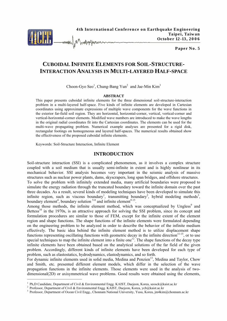
xθ is the rotation of the footing. Rigid Circular Footing : The finite element model for a quarter of the soil-structure interaction system is shown in Figure 7. Poisson ratio (ν ) and the material damping ratio ( dβ ) are assumed to be 0.25 and 0.05, respectively. Figure 8 shows the horizontal and rocking compliances obtained for a rigid circular footing on a homogeneous half-space along with the results by Wei and Veletsos18. The present results are found to be very well agreed with the reference values. Figure 9 presents the results for a rigid disk on a layered half-space. The ratio of the shear wave velocities ( 1 2/s sc c ) of the horizontal layer and the half-space is taken as 0.8, and the ratio of the soil densities ( 1 2/s sρ ρ ) is 0.85. The present results are found to be well correlated with the results by Wong and Luco5. Rigid Square Footing: The FE model used for a quarter of the SSI system is shown in Figure 10. Poisson ratio and the material damping ratio are taken as 0.33 and 0.05. Figure 11 shows the compliance functions of a square footing on a homogeneous half-space along with values obtained by other researchers6,12,16. The other results were obtained using boundary solution methods(by Luco6 and Chow16) and mapped type 3D infinite element method(by Zhao12). Figure 11 shows that the solutions by Luco overestimate the compliance functions and those by Zhao tend to underestimate. The present solutions are found to be close to Chow’s, which are in between those by the other two methods. In Chow’s paper22, it was pointed out that the static compliances( 0oa = ) for square and rectangular footings determined by Chow’s method agree more closely with the exact solutions. Figure 12 shows the compliance functions of a square footing on a layered half-space. The ratio of the shear wave

velocities ( 1 2/s sc c ) is taken on 0.8, and the ratio of th soil densities ( 1 2/s sρ ρ ) is 0.85. The comparisons with Wong and Luco7 are given for the horizontal, vertical and rocking compliance functions. The overall trends of the present solutions agree very well with the reference values, but present results are slightly lower than those by Wong and Luco as in a square footing on a homogeneous medium shown in Figure 12. Rigid Rectangular Footing : A rigid rectangular footing on a horizontal soil layer with an underlying rigid rock is analyzed. The impedance function of the rectangular footing is expressed as

o o( ) = ( + i )(1 2 )staz z dK a K K a C iβ+ , where sta

zK is the vertical static stiffness. HIE and HCIE are used for the horizontal exterior region of the soil layer, while the boundary condition along the interface with the bed rock is taken as fixed. Two cases with different depth ratios( 4h B= and 6B ) are considered. Figure 13 shows the results for the rectangular footings (L/B=2.0, ν=0.33, dβ =0.05) along with the results by Chow17. The present results are observed to be in good agreement with the reference values.

CONCLUSIONS

This paper presents cuboidal dynamic infinite elements for soil-structure interaction analysis in a multi-layered soil medium. Five kinds of cuboidal infinite elements are developed in Cartesian coordinates to model the exterior soil region. The shape functions of the infinite elements contain multiple wave components. Modified wave numbers are introduced to the shape functions in Cartesian coordinates to make the wave lengths in the original radial coordinates fit to the Cartesian coordinates. To verify the effectiveness of the proposed method, the compliance and impedance functions are calculated for a rigid disk, rectangle footings on homogeneous and layered halfspaces. The present results are found to be in good agreement with those obtained by other researchers. The present infinite elements can be effectively used in the SSI analysis of structures with arbitrary geometries subjected to dynamic loads such as earthquake, water waves, blasts and machine vibrations.

REFERENCES

1. J. Lysmer and R.L. Kuhlemeyer, “Finite dynamic model for infinite media”, J. Eng. Mech. Div., ASCE V 95, 859-877(1969) 2. H. Werkle, “Dynamic finite element analysis of three dimensional soil models with transmitting element”, Earthquake Engineering and Structural Dynamics, V 14, 41-60(1986) 3. T.J. Tzong and J. Penzien, “Hybrid modeling of soil-structure interaction in layered media”, Report No. UCB/EERC-83/22, Earthquake Eng. Research Center, UC, Berkeley, CA, (1983) 4. C.H. Chen and J. Penzien, “Dynamic modeling of axisymmetric foundation”, Earthquake Engineering and Structural Dynamics, V 14, 823-840(1986) 5. J.E. Luco, “Impedance functions for a rigid foundation on a layered medium”, Nuclear Eng., V 31, 204-217(1974) 6. H.L. Wong and J.E. Luco, "Dynamic response of a rigid foundation of arbitrary shape", Earthquake Engineering and Structural Dynamics, V 4, 579-587(1976) 7. H.L. Wong and J.E. Luco, "Tables of impedance functions for square foundations on layered media", Soil Dynamics and Earthquake Engineering, V 4, No2, 64-81(1985) 8. G.S. Liou, “Analytical solutions for soil-structure interaction in layered media”, Earthquake Engineering and Structural Dynamics, V 18, 667-686(1989) 9. R.F. Ungless, “An infinite element”, M,S,A. Thesis, University of British Columbia(1973) 10. P. Bettess, “Infinite element”, Int. J. Numer. Methods Eng., V 11 54-64(1977) 11. F. Medina and J. Penzien, “Infinite element for elastodynamic”, Earthquake Engineering and Structural Dynamics., V 10, 699-709(1982) 12. C. Zhao and S. Valliappan, "A Dynamic Infinite Element for Three-Dimensional Infinite Domain Wave Problem". Int. J. Numerical Methods Eng., V 36, 2567-2580(1993) 13. S.C. Yang and C.B. Yun, "Axisymmetric Infinite Elements for Soil-Structure Interaction Analysis", Engineering Structure, V 14, 361-370(1992) 14. C.B. Yun, J.M. Kim and C.H. Hyun, "Axisymmetric infinite element for multi-layered half- space", Int. J. Num. Methods Eng. V 38, 3723-374(1995)

15. D.K. Kim and C.B. Yun "Soil-Structure Interaction Analysis based on Analytical Frequency-Dependent Infinite Element in Time Domain", Struct. Eng. Mech., V 15, 717-733(2003) 16. Y.K. Chow, “Simplified analysis of dynamic response of rigid foundations with arbitrary geometries”, Earthquake Engineering and Structural Dynamics, V 14, 643-653(1986) 17. Y.K. Chow, "Vertical vibration of three-dimensional rigid foundation on layered media", Earthquake Engineering and Structural Dynamics, V 15, 585-594(1987) 18. A.S. Veletsos, Y.T. Wei, “Lateral and rocking vibration of footings”, J. Soil Mechanics and Foundation Division, ASCE, V 97, 1227-1248(1971) 19. A.C. Eringen and E.S. Suhubi, “Elastodynamics”, Academic-Press, London(1975) 20. K.R. Park and E. Watanabe, “Development of 3 dimensional dynamic infinite elements in layered media”, Proceeding of 16th KKCNN Symposium, Gyeongju, Korea(2003)

Table 1. Mappings of the cuboidal infinite elements for quarter model x y z Remark

(1 )jx ξ+ 1

( , )N

j jj

L yη ζ=∑

1( , )

N

j jj

L zη ζ=∑ x-axis ξ -axis

HIE

1( , )

N

j jj

L xη ζ=∑ (1 )jy ξ+

1( , )

N

j jj

L zη ζ=∑ y-axis ξ -axis

VIE 1

( , )N

j jj

L xξ η=∑

1( , )

N

j jj

L yξ η=∑ jz ζ−

HCIE (1 )jx ξ+ (1 )jy η+ 1

( )N

j jj

L zζ=∑

(1 )jx ξ+ 1

( )N

j jj

L yη=∑ jz ζ− x-axis ξ -axis

VCIE

1( )

N

j jj

L xη=∑ (1 )jy ξ+ jz ζ− y-axis ξ -axis

VHCIE (1 )jx η+ (1 )jy ξ+ jz ζ− Note: N= total number of nodes per infinite element; 8 for HIE & VIE, 3 for HCIE & VCIE, 1 for VHCIE.

Table 2 Approximate wave functions in Cartesian coordinates Horizontal layer Underlying halfspace

Exact19 Approximate Exact19 Approximate

Surface waves (2) ( )mH kr ( )( )e , e y ayx ax ik yik x αα − +− + (2) ( )mH kr ( )( )e , e ,ey ay bax ax ik y zik x α µα − + −− +

Body waves (2) ( )mh kR ( ) ( )e , ex bx y byik x ik yβ β− + − + (2) ( )mh kR ( ) ( )( )e , e , ex bx z bzy byik x ik zik yβ ββ− + − +− +

Notes: α and β = geometric damping coefficients for the surface and body waves; axk and bxk = modified wave numbers; a and b = indexes denoting the surface and body waves; and

baµ =coefficient( 2 2a bk k− ) related to the surface wave in the underlying halfspace to z-direction.

HorizontallyLayered Soil

UnderlyingHalfspace

3D IE

3D IE

3D IE

STRUCTURE

Near Field Soil

Far Field Soil

3D FE

3D IE

3D IE

VHCΩ

HCΩ

VΩ

VCΩ

HΩ

HΩ

Z

XY

IΓ

fΓ

Figure 1. 3D soil-structure system Figure 2. Global configuration and infinite regions

HIEO

z HCIE

ξ

ηζ

x

HIE

y

ξ

ηζ

20-noded FEs

HIE

HIE

HCIE

VIE

ξ

η

ζVCIE

ξη

ζ

VHCIE

ξ

ηζ

O'

z y

x

20-noded FEs

(a) Horizontal layered region (b) Underlying halfspace

Figure 3. Geometric mappings

O

FEREGION

i

x

y

nλ( 1)n λ−

( )i xf k x

( 1)n λ+

2 ( )mH kr

2 / kλ π=

xλ

IEREGION

HIE

( )j yf k y

yλ HIE

j

O′

FEREGION

j

z

x

nλ

( 1)n λ−

( )j zf k z

( 1)n λ+ 2 ( )mh kR

λ

zλ

IEREGION

VIE

(a) Modified wave length in horizontal layer (b) Modified wave length in underlying halfspace

Figure 4 Wave propagations in Cartesian coordinates

XY

Z

FE

STR

HIEHIE

HCIE

YX

Z

STR

HCIE

HIE

HIE

VIE

FE

VCIE

VCIE

(a) Surface waves on the surface (b) Body waves(P) in an elastic halfspace

Figure 5. Examples of wave propagations simulated using the present infinite elements due to a vertical harmonic excitation

2B

M i te ω

H ei tω

V ei tω

h (1) (1) (1), , scν µ

(2) (2) (2), , scν µ Rigid Rock

2B, ,cν µ

V i te ω

h

(a) Rigid footing on layered halfspace (b) Rigid footing with bed rock

Figure 6. Geometric definition of various numerical examples

FEΩ

IEΩ

B

D

1, 1sc ρ

2, 2sc ρ

Figure 7. FE model for a disk footing on the surface: a quarter model

0 1 2 3ao=ωB/cs

0

0.05

0.1

0.15

0.2

0.25

Re(CHH)

Im(CHH)

Veletsos(1971)

This study

0 1 2 3

ao=ωB/cs

0

0.1

0.2

0.3

0.4

Re(CMM)

Im(CMM)

(a) Horizontal compliance (b) Rocking compliance

Figure 8. Compliance functions of a rigid disk on homogeneous half-space

0 1 2 3ao=ωB/cs1

0

0.05

0.1

0.15

0.2

Re(CHH)

Im(CHH)

Luco(1974)

This study

0 1 2 3

ao=ωB/cs1

0

0.1

0.2

0.3

0.4

Re(CMM)

Im(CMM)

(a) Horizontal compliance (b) Rocking compliance

Figure 9. Compliance functions of a rigid disk on a layered half-space (h/B=1.0)

IEΩ

h

B

1D

L

FEΩ

1, 1sc ρ

2, 2sc ρ

2D

IEΩ

IEΩ

Figure 10. FE model for a rectangular footing on the surface: a quarter model

0 1 2 3ao=ωΒ/cs

0

0.05

0.1

0.15

0.2

Re(CHH)

Im(CHH)

This studyLuco(1976)Chow(1986)Zhao(1993)

0 1 2 3

ao=ωΒ/cs

0

0.05

0.1

0.15

Re(CVV)

Im(CVV)

(a) Horizontal compliance (b) Vertical compliance

0 0.5 1 1.5 2ao=ωΒ/cs

0

0.05

0.1

0.15

0.2

0.25

Re(CMM)

Im(CMM)

(c) Rocking compliance

Figure 11. Compliance functions of a rigid square footing on a homogeneous half-space

0 1 2 3ao=ωΒ/cs1

0

0.05

0.1

Re(CVV)

Im(CVV)

0 1 2 3

ao=ωΒ/cs1

0

0.05

0.1

0.15

0.2

Re(CHH)

Im(CHH)

Luco(1985)

This study

(a) Horizontal compliance (b) Vertical compliance

0 0.5 1 1.5 2ao=ωΒ/cs1

0

0.05

0.1

0.15

0.2

Re(CMM)

Im(CMM)

(c) Rocking compliance

Figure 12. Compliance functions of a rigid square footing on a layered half-space (h/B=1.0)

0 1 2 3ao=ωB/cs

0

0.5

1KVV

CVV

This study

Chow(1987)

0 1 2 3

ao=ωB/cs

0

0.5

1KVV

CVV

(a) Vertical impedance (h/B=4.0) (b) Vertical impedance ( h/B=6.0)

Figure 13. Vertical impedances of rectangular footings on a layer with a bed rock