reliability assessment of self centering steel...
TRANSCRIPT
4th International Conference on Earthquake EngineeringTaipei, Taiwan
October 12-13, 2006
Paper No. 102
RELIABILITY ASSESSMENT OF SELF-CENTERING STEELMOMENT FRAME SYSTEMS
Mark Dobossy1, Erik VanMarcke2, Maria Garlock3
ABSTRACT
Researchers from various institutions have recently developed innovative steel moment frame systemsfor earthquake-resistant design that, following a major earthquake, have the potential to reduce or elim-inate structural damage and return to its original vertical position (i.e. self-center). As the developmentof these steel moment frames with self-centering behavior progresses, it will be necessary to spec-ify design parameters and a workable design method. This will require a good understanding of thesensitivity of the structure to changes in these parameters as well as the reliability of structures builtbased on the proposed method. This research investigates a risk assessment methodology (using MonteCarlo simulation) of the seismic response of self-centering steel moment frame prototype buildings.First, we perform a series of conditional seismic reliability assessments of the structure. Syntheticallygenerated earthquakes with magnitudes and distances within narrow ranges that are consistent withground-motion attenuation curves for a specified return period a specific building site are generatedand applied to the structure, and peak relative rotations between the beam and column are recorded.This data is then used to generate demand curves (with respect to relative rotation) for the structure.From these, one can assess the risk of a particular design at a specific site having significant structuraldamage. Next, a study is performed to determine the capacity of gap relative rotation in relation to limitstate attainment. The results of both studies are then combined to determine the overall reliability of thestructure which be used to develop a reliability-based seismic design procedure for these self-centeringsteel moment frames.
Keywords: self-centering, moment frames, reliability, performance-based design
INTRODUCTION
Innovative self-centering steel moment resisting frame (SC-MRF) systems for earthquake-resistant de-sign have recently been developed. Following a major earthquake, this system has the potential to reduceor eliminate structural damage and return to its original vertical position (i.e. self-center). In a SC-MRF,post-tensioned strands (or bars) run parallel to the beam and compress the beam against the column face.When the moment in the connection overcomes the moment resisted by the post-tensioned strands, a
1Graduate Student, Dept. of Civil and Environmental Engineering, Princeton University, Princeton, NJ 08544,[email protected]
2Professor, Dept. of Civil and Environmental Engineering, Princeton University, Princeton, NJ 08544,[email protected]
3Assistant Professor, Dept. of Civil and Environmental Engineering, Princeton University, Princeton, NJ 08544,[email protected]

relative rotation develops between the beam and column (θr). More details on this system can be foundin Ricles et al. (2001); Garlock et al. (2005); Rojas et al. (2005); Christopoulos et al. (2002a).
This paper investigates a reliability assessment procedure for the seismic response of SC-MRFs. Thismethodology involves calculating the seismic demands on the SC-MRF and the structural capacity re-lated to a specific limit state. In this paper, the limit state of strand yielding is used as a measure ofcapacity to illustrate the reliability assessment procedure. Other limit states can be used in mannerssimilar to that shown here.
θr, as shown in Figure 1, is selected as the measure of demand for this study since in a SC-MRF, θr canbe related to many limit states such as strand yielding, beam buckling and energy dissipation device limitstates. Two methods are proposed for developing the seismic demands on the prototype structure: a sitecharacteristic method and a scenario method where magnitudes and distances of earthquakes are limitedto a narrow ranges. Both methods use Monte Carlo simulations with the distance to and the magnitudeof the seismic event as random variables. The prototype SC-MRF is subjected to a large number ofearthquakes using randomly generated ground motions consistent with the site or scenario. At the end ofeach non-linear analysis, the peak θr is recorded.
contact surface and center of rotation
d2
M
P
V
θr
∆gap
Figure 1: SC-MRF Connection Detail.
Using the probabilistic demand and capacity curves generated through the simulations, the combinedprobability of the demand exceeding the capacity is calculated for every floor of the prototype frame.Such a method can be used to develop a reliability performance-based design approach for SC-MRFsystems.
STRUCTURAL MODEL
The two primary methods of modeling SC-MRF systems involve the use of explicit gap elements, and theuse, at each connection, of rotational springs that model the connection moment-rotation behavior. Ananalysis was performed by the authors, to determine the advantages and disadvantages of each method(Dobossy et al., 2006). It was found that while the rotational spring model has some limitations, owingto its computational efficiency, the rotational spring model is the best method for a study involvingthousands of simulations such as the one at hand. Thus, the rotational spring model was chosen for thisstudy.
The rotational spring model is a simplified approach to modeling SC-MRF systems where a rotationalspring with a moment-rotation behavior representative of the behavior seen at a SC-MRF connectionis inserted between the beam and column (Christopoulos et al., 2002a; Tsai et al., 2005; Priestley etal., 1999). A schematic of a typical inner column connection model is shown in Figure 2. In order toproperly simulate the depth of the columns, slaved nodes are used to push the connection out from the
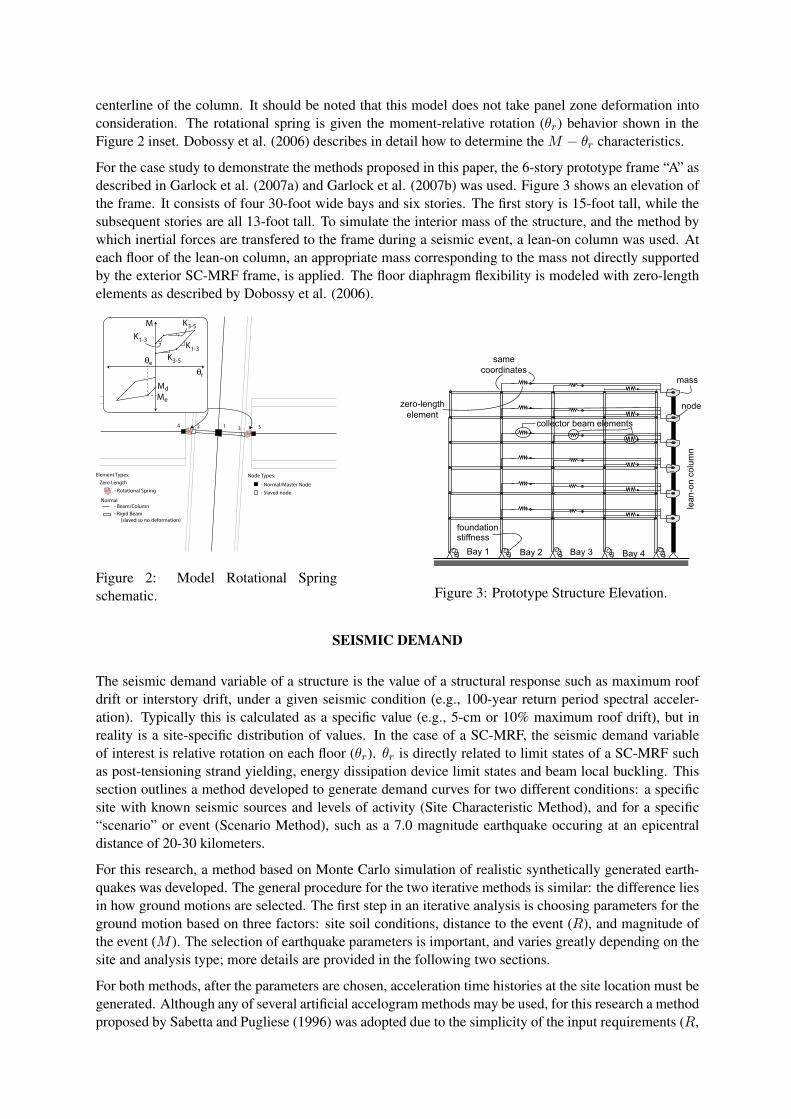
centerline of the column. It should be noted that this model does not take panel zone deformation intoconsideration. The rotational spring is given the moment-relative rotation (θr) behavior shown in theFigure 2 inset. Dobossy et al. (2006) describes in detail how to determine the M − θr characteristics.
For the case study to demonstrate the methods proposed in this paper, the 6-story prototype frame “A” asdescribed in Garlock et al. (2007a) and Garlock et al. (2007b) was used. Figure 3 shows an elevation ofthe frame. It consists of four 30-foot wide bays and six stories. The first story is 15-foot tall, while thesubsequent stories are all 13-foot tall. To simulate the interior mass of the structure, and the method bywhich inertial forces are transfered to the frame during a seismic event, a lean-on column was used. Ateach floor of the lean-on column, an appropriate mass corresponding to the mass not directly supportedby the exterior SC-MRF frame, is applied. The floor diaphragm flexibility is modeled with zero-lengthelements as described by Dobossy et al. (2006).
Element Types:
Zero Length
- Rotational Spring
- Beam/Column
- Rigid Beam
(slaved so no deformation)
Normal
Node Types:
- Normal/Master Node
- Slaved node
12 34 5
θr
θe
M
K1-3
K3-5
K3-5
K1-3
Md
Me
Figure 2: Model Rotational Springschematic.
node
mass
foundation
stiffness
lea
n-o
n c
olu
mn
Bay 1 Bay 2 Bay 3 Bay 4
collector beam elements
same
coordinates
zero-length
element
Figure 3: Prototype Structure Elevation.
SEISMIC DEMAND
The seismic demand variable of a structure is the value of a structural response such as maximum roofdrift or interstory drift, under a given seismic condition (e.g., 100-year return period spectral acceler-ation). Typically this is calculated as a specific value (e.g., 5-cm or 10% maximum roof drift), but inreality is a site-specific distribution of values. In the case of a SC-MRF, the seismic demand variableof interest is relative rotation on each floor (θr). θr is directly related to limit states of a SC-MRF suchas post-tensioning strand yielding, energy dissipation device limit states and beam local buckling. Thissection outlines a method developed to generate demand curves for two different conditions: a specificsite with known seismic sources and levels of activity (Site Characteristic Method), and for a specific“scenario” or event (Scenario Method), such as a 7.0 magnitude earthquake occuring at an epicentraldistance of 20-30 kilometers.
For this research, a method based on Monte Carlo simulation of realistic synthetically generated earth-quakes was developed. The general procedure for the two iterative methods is similar: the difference liesin how ground motions are selected. The first step in an iterative analysis is choosing parameters for theground motion based on three factors: site soil conditions, distance to the event (R), and magnitude ofthe event (M ). The selection of earthquake parameters is important, and varies greatly depending on thesite and analysis type; more details are provided in the following two sections.
For both methods, after the parameters are chosen, acceleration time histories at the site location must begenerated. Although any of several artificial accelogram methods may be used, for this research a methodproposed by Sabetta and Pugliese (1996) was adopted due to the simplicity of the input requirements (R,
M and soil depth) and the realistic nonstationary accelograms it generates. However, the attenuationrelationships developed by Sabetta and Pugliese (1996) were based on limited seismic data (magnitude4.4 to 6.8) from Italian quakes. To be applicable to a hypothetical site located in southern California,the attenuation (mainly of Arias Intensity) was updated using the empirical relationship developed byTravasarou et al. (2003).
Each time history of the acceleration is then applied at the base of the structure. In this research, theOpenSees software was used for the time-history analysis of the structural response (McKenna & Fenves,2006). At each connection, the envelope of maximum and minimum θr is recorded for each groundmotion. Many simulated ground motions for the site and its seismic setting are generated. After a largenumber of simulations are performed, a distribution is fitted to the data at each connection, resulting in ademand curve for the connection relative rotation.
Site Characteristic Method
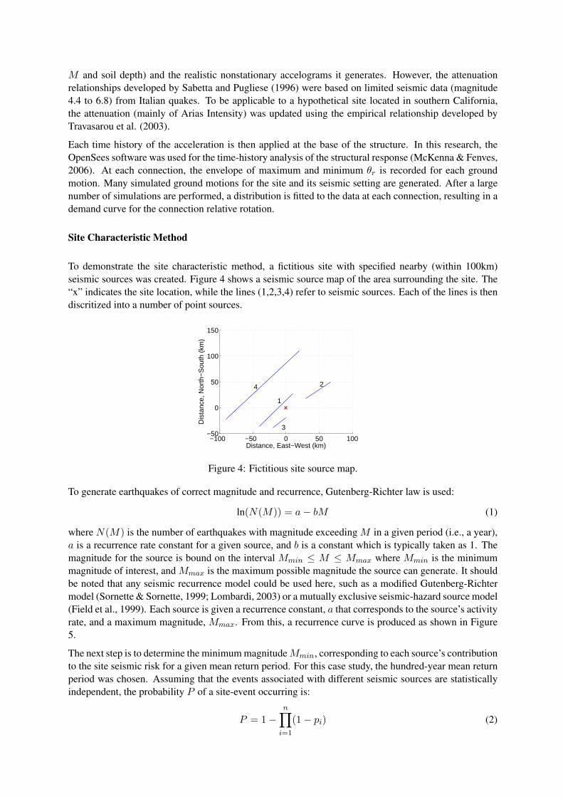
To demonstrate the site characteristic method, a fictitious site with specified nearby (within 100km)seismic sources was created. Figure 4 shows a seismic source map of the area surrounding the site. The“x” indicates the site location, while the lines (1,2,3,4) refer to seismic sources. Each of the lines is thendiscritized into a number of point sources.
−100 −50 0 50 100−50
0
50
100
150
Distance, East−West (km)
Dis
tanc
e, N
orth
−S
outh
(km
)
1
2
3
4
Figure 4: Fictitious site source map.
To generate earthquakes of correct magnitude and recurrence, Gutenberg-Richter law is used:
ln(N(M)) = a− bM (1)
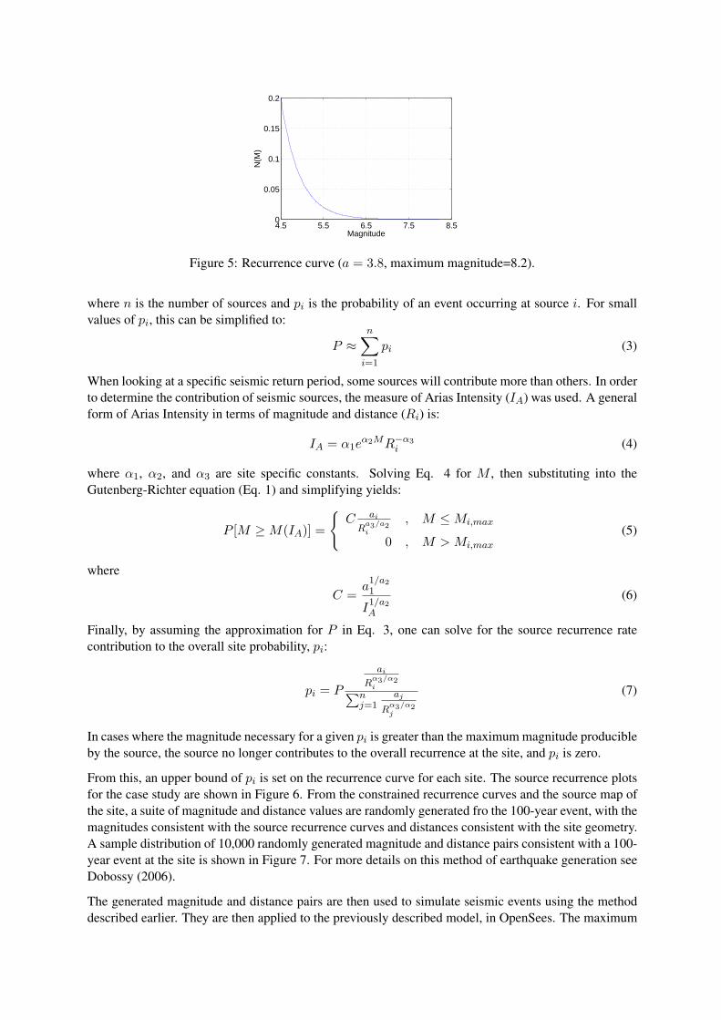
where N(M) is the number of earthquakes with magnitude exceeding M in a given period (i.e., a year),a is a recurrence rate constant for a given source, and b is a constant which is typically taken as 1. Themagnitude for the source is bound on the interval Mmin ≤ M ≤ Mmax where Mmin is the minimummagnitude of interest, and Mmax is the maximum possible magnitude the source can generate. It shouldbe noted that any seismic recurrence model could be used here, such as a modified Gutenberg-Richtermodel (Sornette & Sornette, 1999; Lombardi, 2003) or a mutually exclusive seismic-hazard source model(Field et al., 1999). Each source is given a recurrence constant, a that corresponds to the source’s activityrate, and a maximum magnitude, Mmax. From this, a recurrence curve is produced as shown in Figure5.
The next step is to determine the minimum magnitude Mmin, corresponding to each source’s contributionto the site seismic risk for a given mean return period. For this case study, the hundred-year mean returnperiod was chosen. Assuming that the events associated with different seismic sources are statisticallyindependent, the probability P of a site-event occurring is:
P = 1−n∏
i=1
(1− pi) (2)
4.5 5.5 6.5 7.5 8.50
0.05
0.1
0.15
0.2
Magnitude
N(M
)Figure 5: Recurrence curve (a = 3.8, maximum magnitude=8.2).
where n is the number of sources and pi is the probability of an event occurring at source i. For smallvalues of pi, this can be simplified to:
P ≈n∑
i=1
pi (3)
When looking at a specific seismic return period, some sources will contribute more than others. In orderto determine the contribution of seismic sources, the measure of Arias Intensity (IA) was used. A generalform of Arias Intensity in terms of magnitude and distance (Ri) is:
IA = α1eα2MR−α3
i (4)
where α1, α2, and α3 are site specific constants. Solving Eq. 4 for M , then substituting into theGutenberg-Richter equation (Eq. 1) and simplifying yields:
P [M ≥ M(IA)] =
{C ai
Ra3/a2i
, M ≤ Mi,max
0 , M > Mi,max
(5)
where
C =a
1/a2
1
I1/a2
A
(6)
Finally, by assuming the approximation for P in Eq. 3, one can solve for the source recurrence ratecontribution to the overall site probability, pi:
pi = P
ai
Rα3/α2i∑n
j=1aj
Rα3/α2j
(7)
In cases where the magnitude necessary for a given pi is greater than the maximum magnitude producibleby the source, the source no longer contributes to the overall recurrence at the site, and pi is zero.
From this, an upper bound of pi is set on the recurrence curve for each site. The source recurrence plotsfor the case study are shown in Figure 6. From the constrained recurrence curves and the source map ofthe site, a suite of magnitude and distance values are randomly generated fro the 100-year event, with themagnitudes consistent with the source recurrence curves and distances consistent with the site geometry.A sample distribution of 10,000 randomly generated magnitude and distance pairs consistent with a 100-year event at the site is shown in Figure 7. For more details on this method of earthquake generation seeDobossy (2006).
The generated magnitude and distance pairs are then used to simulate seismic events using the methoddescribed earlier. They are then applied to the previously described model, in OpenSees. The maximum

6.5 7 7.5 8 8.5 9 9.50
0.005
0.01
0.015
0.02
0.025
0.03
0.035
Magnitude
Rec
urra
nce
Source 1
Source 3
Source 2 Source 4
Figure 6: Recurrence curves for case studysources.
0 50 1006.5
7
7.5
8
8.5
9
9.5
Distance (km)
Mag
nitu
de
Figure 7: Seismic event moment and distancedistribution.
and minimum rotation of a connection at an interior bay and a connection at an exterior bay are recordedfor each ground motion.
A distribution is fitted to the recorded data. It was found that a lognormal distribution fit the rotationdata well. Figures 8 and 9 show the resulting data and distribution fit for the probability density, andprobability curve for an interior connection on the second floor. Similar curves are generated for allfloors and connection types. The data and probability of interest is the tail of the distribution, rotationsgreater than 0.025 radians. As can be seen in Figure 9, the lognormal distribution fit correlates well tothe tail of the distribution.
0 0.05 0.1 0.150
10
20
30
40
50
Rotation (rad)
Den
sity
Rotation Data
Lognormal Fit
Figure 8: Site characteristic method PDF dataand fit.
0 0.05 0.1 0.15
0.00010.001 0.01
0.1 0.25
0.75 0.9
0.99 0.999 0.9999
Rotation (rad)
Pro
babi
lity
Rotation Data
Lognormal Fit
Figure 9: Site characteristic methodexceedance-probability curve data andfit.
Scenario (bin) Method
In many cases, the detailed seismic hazard information necessary to apply the “site characteristic method”may not be available. In these cases, a different approach must be taken to assess the seismic demandon the structure. One such approach is a scenario based approach, where one or more ranges of eventmagnitudes and distances are studied. For example one might ask, what is the structural demand for theprototype structure, given an earthquake of magnitude 7.0-7.5 at a distance of 20-30km. This can alsobe thought of as looking at a specific magnitude and distance bin. In this way, one can study specifictypes of events which a structure may see during its service life. In order to demonstrate generation of ademand curve, the forementioned example will be used.
First, a number of random magnitude and distance pairs are chosen, uniformly distributed over the mag-

nitude and distance range of interest. Figure 10 shows the 10,000 pairs that were used for this case study.As with the “site characteristic method”, these magnitude and distance pairs are then used to generatesynthetic earthquakes applied to the structural model in OpenSees.
0 10 20 30 40 50 606.5
7
7.5
8
8.5
9
9.5
Distance (km)
Mag
nitu
de
(a) “Bins” of scenarios.
20 22 24 26 28 307
7.1
7.2
7.3
7.4
7.5
Distance (km)
Mag
nitu
de
(b) Distribution of 10,000 seismic events in bin se-lected
Figure 10: Scenario method seismic event distribution.
Next, a distribution is fitted to the data. When ranges of magnitude and distance are relatively narrow, theWeibull distribution typically fits well. Figures 11 and 12 show the probability density and cumulativeprobability curves for the data produced in the example, along with the Weibull fit. As with the sitecharacteristic method, the fit correlates well to the tail of the distribution which is the area of greatestinterest.
0 0.005 0.01 0.015 0.020
20
40
60
80
100
120
Connection Rotation (rad)
Den
sity
Rotation Data
Weibull Fit
Figure 11: Scenario method PDF data and fit.
0 0.005 0.01 0.015 0.02
0.00010.001 0.01
0.1 0.25 0.5 0.75 0.9
0.99 0.999 0.9999
Data
Pro
babi
lity
Simulation Data
Weibull Fit
Figure 12: Scenario method probability curvedata and fit.
CAPACITY
To determine the reliability of a structure under seismic loading, one needs to know the demand placedon the structure in relation to the structure’s capacity. Capacity is the point at which a given structuralresponse will cause some limit state to be reached in the structure. In some cases, the capacity of a givenstructural response may be a known value, however in many cases, uncertainty is involved. The responselimit, or capacity, will be a single point for situations lacking uncertainty, and will be characterized by aprobability distribution otherwise.
For the case study, the limit state of interest is post-tensioning strand yielding, and the measured responseis the gap rotation whose demand was determined in the previous section. As floors of a SC-MRF arepushed laterally, in a seismic event, gap opening at the connections causes an expansion of the floorsystem, as shown in Figure 13. As the floor expands, the post-tensioning strands are stretched. A closed

form solution was derived which shows the average floor gap relative rotation at which strand yieldingtakes place, θr,s:
θr,s =Ns(ty − to)
2d2· kb + ks
kbks(8)
where Ns is the number of strands, ty is the force in one strand when yielding takes place, to is theinitial (average) post-tensioning force per strand, d2 is the distance from the center of rotation to thebeam centerline (Figure 1), kb is the axial stiffness of the beam and ks is the axial stiffness of the strands(Garlock et al., 2007a).
(a)
(b)
(c)
(d)
θr (typical)∆gap 2∆gap−∆gap
−2∆gap
collector beams
fcb
Figure 13: Expanding nature of SC-MRF floors.
The two main sources of uncertainty for strand yielding capacity are the yield force, ty (material uncer-tainty) and the original post-tensioning force, to (construction uncertainty). Current data on steel yieldstrength variability shows that steel yield stress for 50ksi steel is typically normally distributed with amean of 50.4ksi, and a standard deviation of 4.53ksi (State, 2000). No data was available for very-high-strength steel used for post-tensioning strands, so the values were extrapolated from the FEMA reportfor this example. The nominal ultimate stress for the strands is 270ksi. It is assumed that the yield stressis equal to 90% of the ultimate stress. Thus, the distribution of strand yield stress was assumed to benormally distributed, with a mean of 244.9ksi and standard deviation of 22.01ksi. No data was found forthe uncertainty in post-tensioning at a construction site, so for this example it was assumed that givena target post-tensioning force, to, the distribution of the post-tensioning force was normal with mean toand standard deviation 0.05to. In this simple example, using the stiffness, post-tensioning, and geometryvalues for the second floor, yields a normal distribution with a mean µ of 0.0478 radians and a standarddeviation σ of 0.0085 radians, as shown in Figure 14
0 0.02 0.04 0.06 0.08 0.10
0.2
0.4
0.6
0.8
1
θr
P[S
tran
d Y
ield
ing
| θr]
Figure 14: CDF of tensioning strand yielding in terms of average floor joint rotation.
OVERALL RELIABILITY
Once the capacity and demand distributions have been determined, determining the probability of limitstate attainment for the given demand parameters (i.e., corresponding to the one-hundred year earthquake
at the building site) is done by convolving the distributions of capacity and demand. The probability thatthe limit-state capacity is less than the demand is the “probability of failure”:
P[Cap < Dem] =∑
all i
P[Cap < Demi] · P[Demi] (9)
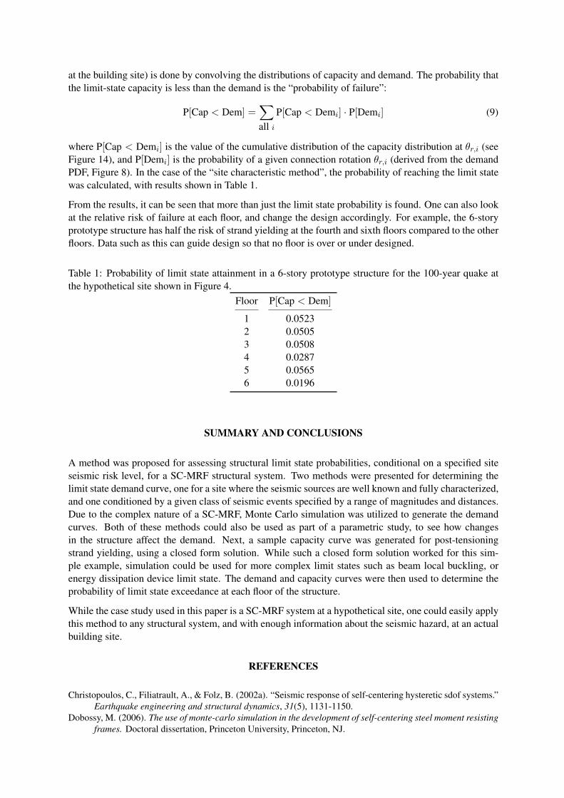
where P[Cap < Demi] is the value of the cumulative distribution of the capacity distribution at θr,i (seeFigure 14), and P[Demi] is the probability of a given connection rotation θr,i (derived from the demandPDF, Figure 8). In the case of the “site characteristic method”, the probability of reaching the limit statewas calculated, with results shown in Table 1.
From the results, it can be seen that more than just the limit state probability is found. One can also lookat the relative risk of failure at each floor, and change the design accordingly. For example, the 6-storyprototype structure has half the risk of strand yielding at the fourth and sixth floors compared to the otherfloors. Data such as this can guide design so that no floor is over or under designed.
Table 1: Probability of limit state attainment in a 6-story prototype structure for the 100-year quake atthe hypothetical site shown in Figure 4.
Floor P[Cap < Dem]
1 0.05232 0.05053 0.05084 0.02875 0.05656 0.0196
SUMMARY AND CONCLUSIONS
A method was proposed for assessing structural limit state probabilities, conditional on a specified siteseismic risk level, for a SC-MRF structural system. Two methods were presented for determining thelimit state demand curve, one for a site where the seismic sources are well known and fully characterized,and one conditioned by a given class of seismic events specified by a range of magnitudes and distances.Due to the complex nature of a SC-MRF, Monte Carlo simulation was utilized to generate the demandcurves. Both of these methods could also be used as part of a parametric study, to see how changesin the structure affect the demand. Next, a sample capacity curve was generated for post-tensioningstrand yielding, using a closed form solution. While such a closed form solution worked for this sim-ple example, simulation could be used for more complex limit states such as beam local buckling, orenergy dissipation device limit state. The demand and capacity curves were then used to determine theprobability of limit state exceedance at each floor of the structure.
While the case study used in this paper is a SC-MRF system at a hypothetical site, one could easily applythis method to any structural system, and with enough information about the seismic hazard, at an actualbuilding site.
REFERENCES
Christopoulos, C., Filiatrault, A., & Folz, B. (2002a). “Seismic response of self-centering hysteretic sdof systems.”Earthquake engineering and structural dynamics, 31(5), 1131-1150.
Dobossy, M. (2006). The use of monte-carlo simulation in the development of self-centering steel moment resistingframes. Doctoral dissertation, Princeton University, Princeton, NJ.
Dobossy, M., Garlock, M., & VanMarcke, E. (2006). Comparison of two self-centering steel moment framemodeling techniques: explicit gap models, and non-linear rotational spring models. Proceedings of the 4thInternational Conference on Earthquake Engineering. Taipei, Taiwan.
Field, E., Jackson, D., & Dolan, J. (1999, June). “A mutually consistent seismic-hazard source model for southerncalifornia.” Bulletin of the Seismological Society of America, 89(3), 559-578.
Garlock, M., Ricles, J., & Sause, R. (2005). “Experimental studies on full-scale post-tensioned steel connections.”Journal of Structural Engineering, 131(3), 438-448.
Garlock, M., Ricles, J., & Sause, R. (2007b). “Analytical modeling and seismic response of post-tensioned steelframes.” Journal of Structural Engineering. (submitted for publication)
Garlock, M., Sause, R., & Ricles, J. (2007a). “Behavior and design of post-tensioned steel frames.” Journal ofStructural Engineering. (submitted for publication)
Lombardi, A. m. (2003, October). “The maximum likelihood estimator of b-value for mainshocks.” Bulletin ofthe Seismological Society of America, 93(5), 2082-2088.
McKenna, F., & Fenves, G. L. (2006). Opensees 1.7.0. Computer Software. UC Berkeley, Berkeley, CA.Priestley, M. J. N., Sritharan, S., Conley, J., & Pampanin, S. (1999). “Preliminary results and conclusions from the
presss five-story precast concrete test building.” PCI Journal, 44(6), 42-67.Ricles, J., Sause, R., Garlock, M., & Zhao, C. (2001). “Posttensioned seismic-resistant connections for steel
frames.” Journal of Structural Engineering, 127(2), 113-121.Rojas, P., Ricles, J., & Sause r. (2005). “Seismic performance of post-tensioned steel moment resisiting frames
with friction devices.” Journal of Structural Engineering, 131(4).Sabetta, F., & Pugliese, A. (1996, April). “Estimation of response spectra and simulation of nonstationary earth-
quake ground motions.” Bulletin of the Seismological Society of America, 86(2), 337-352.Sornette, D., & Sornette, A. (1999, August). “General theory of the modified gutenberg-richter law for large
seismic moments.” Bulletin of the Seismological Society of America, 89(4), 1121-1130.State of the art report on base metals and fracture. (2000). Federal Emergency Management Agency, Report
Number FEMA-355a, Washington, D.C.Travasarou, T., Bray, J., & Abrahamson, N. (2003). “Emperical attenuation relationship for arias intensity.”
Earthquake Engineering and Structural Dynamics, 32, 1133-1155.Tsai, K.-C., Chou, C.-C., & Jhuang, S.-J. (2005). Seismic response of structural systems using self-centering
connections. US-Taiwan Workship on Self-Centering Structural Systems.