Currency Crises and Foreign Credit in Emerging Markets:

Credit Crunch or Demand Effect?

Galina Hale∗

Yale University

Carlos Arteta

Board of Governors of the Federal Reserve System

June 2006

Abstract

Currency crises of the past decade highlighted the importance of balance–sheet effects of largedevaluations. In credit constrained markets such effects would lead to further decline in credit.Controlling for a host of fundamentals, we find about a decline in foreign credit to emergingmarket private firms of about 30% following large depreciations that lasts between four months(for the financial firms) and two years (for non–financial non–exporting firms). We identify theeffects of large depreciations on demand and supply of credit and find that both demand andsupply decline after crises. However, once we account for the effects of sovereign debt crises,which mostly reduce demand for credit, we find that only decline in supply is significant in theaftermath of currency crisis: the market value of the debt falls by about 13% in the first sixmonths after a large depreciation, which translates into about 4% decline in credit due to acredit crunch.

JEL classification: F34, F32, G32

Key words: currency crises, credit rationing, balance–sheet effects, credit constraints, original sin

∗Corresponding author. Contact: Department of Economics, Yale University, PO Box 208268, New Haven CT06520-8268, galina.hale@yale.edu. We are grateful to Emily Breza, Rachel Carter, Yvonne Chen and Damian Rozofor outstanding research assistance. Anusha Chari, Jose Scheinkman, Martin Schneider and the participants of theSCCIE conference on ”Firms in Emerging Markets” provided most helpful comments. All errors are ours. The viewsin this paper are solely the responsibility of the authors and should not be interpreted as reflecting the views of theBoard of Governors of the Federal Reserve System or any other person associated with the Federal Reserve System.

1

1 Introduction

Recent financial crises in emerging markets brought to light currency–related balance–sheet prob-

lems. The literature on the balance–sheet effects has shown that these effects can lead to a decline

in investment.1 A popular view seems to be that this decline in investment is driven by a credit

crunch. This credit crunch could come from the decline in the domestic banking sector in the

aftermath of crises, but could also be driven by the unwillingness of foreigners to provide credit. In

this paper, we focus on the credit provided to emerging markets’ private firms by foreign creditors.2

To our knowledge, there is no systematic evidence on the effects of currency crises on the demand

and supply of foreign credit to emerging market firms. This paper aims to provide such an analysis.

The so–called “original sin” literature argues that most emerging market borrowers cannot borrow

abroad in their own currency;3 as a result, they may accumulate large foreign–currency liabilities.

If the asset side of these borrowers’ balance sheets is denominated primarily in local currency,

large depreciation of a local currency leads to a large reduction in a company’s net worth and

potentially to solvency problems. Thus, according to standard credit rationing argument (Stiglitz

and Weiss, 1981; Calomiris and Hubbard, 1990; Mason, 1998), it is natural to expect that foreign

lenders will reduce the supply of credit to these borrowers.

There is a number of reasons to believe that the firms will also lower their demand for credit in gen-

eral and foreign credit in particular. First, most developing countries that experience financial crises

also suffer from serious contractions in aggregate demand (Gupta, Mishra, and Sahay, 2003; Hutchi-

son and Noy, 2002), which would increase firms’ inventory and reduce their demand for credit. This

decline in aggregate demand will mostly affect the firms that sell their product domestically. Ex-

porting firms, on the other hand, will experience an increase in their foreign currency revenues

relative to their predominantly domestic currency denominated operating costs.4 Thus, their earn-

1See, for example, Aghion, Bacchetta, and Banerjee (2001), Aghion, Bacchetta, and Banerjee (forthcoming),Cespedes, Chang, and Velasco (2003).

2We focus on emerging markets because the exchange rate movements appear to be more destabilizing in developingcountries than in industrial countries (Ahmed, Gust, Kamin, and Huntley, 2002).

3This point was first raised by Eichengreen, Hausmann, and Panizza (2002).4In fact, Bris and Koskinen (2002) in their model show that this effect could be a reason for competitive devalu-

ations.

2

ings will go up and they will be inclined to demand less credit.5 Finally, all firms, especially those

selling domestically, might decide to reduce the currency mismatch in their balance sheets and

increase their borrowing in domestic currency. Since they are unable to do that on foreign capital

markets, they will increase demand for domestic funds and reduce their demand for foreign credit.

This last development, however, should increase demand for foreign credit by financial sector firms

and may cancel out in the aggregate.

Using firm–level data on foreign bond issuance and foreign syndicated bank loan contracts, we group

the firms into financial and non–financial exporting and non–exporting sectors.6 For each sector,

we calculate the total amount that they borrowed on the bond market or from bank syndicates in

each month. We do this for 34 emerging markets between 1981 and 2004. We then analyze how

this aggregate measure of credit is affected by large currency depreciations. We also construct a

number of indicators that describe various aspects of each country’s economy as well as factors

that affect world supply of capital to emerging markets, which we use as control variables. Since

foreign credit to the country could be conditional on the country having agreement with the IMF,

we include this indicator in our list of control variables. In addition, we control for the systemic

“sudden stops” in foreign credit to the country (Calvo, Izquierdo, and Talvi, 2006), which helps us

control for reverse causality.

Using fixed–effect panel data regressions, we find that there is indeed a significant decline in credit

to emerging market firms (measured either in US dollars or in local currency) in the aftermath

of large currency depreciations. Controlling for a host of fundamentals and for the effects of debt

crises, we find that credit falls by about 30%, compared to the country mean for total private sector

borrowing, in the first year after a large depreciation, and about 15% decline in the second year.

As we expected, this decline in the foreign credit is most persistent for the non–exporting firms.

For financial firms the decline in credit seems to subside after four month, while for the exporters

it lasts about 8 months on average. We find some reduction in credit up to three months before

the large depreciation; however, it is not significant in most specifications.

5Real depreciation is more important than nominal depreciation for this effect. However, as Burstein, Eichenbaumand Rebelo (2002; 2004) show, prices take awhile to catch up with exchange rates when depreciations are large;therefore, real and nominal depreciations go hand in hand.

6We exclude from our analysis all the firms that are foreign–owned.

3

By separating demand factors from supply factors, and using a proxy for the price of credit, we

are able to identify separately the demand and the supply of credit and see whether the decline

in credit that we document comes from the demand or the supply side. Because we do not have

good exclusion restrictions for the supply equation, we assume that supply of credit for each firm

is perfectly elastic at a given price. We then estimate the demand equation without imposing

restrictions on its slope with respect to our measure of price. At first it appears as though most

of the decline in credit is due to the reduction in demand. However, once we control for sovereign

debt crises, which mostly reduce demand for credit (Arteta and Hale, 2006), we find that only

the reduction in the supply of credit due to large currency depreciations remains significant. This

reduction is limited to the first 6 months after a large depreciation and is equal to 13% decline in

the market value of bonds, which translated, given our estimate of the demand elasticity, to only

about 4% decline in credit.

Thus, we find systematic evidence of foreign credit crunch in the aftermath of large depreciations

that lasts about half a year after the event. This foreign credit crunch is important as it extends to

the entire private sector of the economy, thus limiting the overall credit availability in the country.

In that, our findings are consistent with the evidence presented in Desai, Foley, and Forbes (2004),

which compares access to credit for multinational and domestic firms, and in Blalock, Gertler, and

Levine (2004), which shows the evidence of credit crunch after crisis in Indonesia. Our results also

support the view that investment declines after currency crises and help explain this decline by

providing evidence of the credit crunch.

The remainder of the paper is organized as follows. Part two describes empirical approach of the

paper and the data. Part three presents the results of the empirical analysis. Part four concludes.

2 Empirical approach and data sources

We begin by analyzing the reduced–form specification, which excludes the cost of credit. This

allows us to use a much longer time period and address the differences in the effects of currency

crises on the borrowing of firms from different sectors. As we will discuss later, estimating the

demand and supply effect requires a proxy for the cost of credit that limits our sample size and

4

does not vary by sector.

2.1 Reduced form specification

In order to test for a decline in credit in the aftermath of a large currency depreciation, we estimate

the following reduced–form equation, using regressions with fixed effects:

qit = αi + αt + β0 dit +K∑

τ=1

γτ zτit + X′itη + εit, (1)

where qit is a measure of credit, αi is a set of country fixed effects absorbing the effect of initial

conditions, αt is a set of year fixed effects absorbing the effect of common trend, dit is an indicator

of a devaluation/depreciation month, zτit is an indicator that depreciation occurred more than

τ − 1 but less than τ years ago (we set K = 3), Xit is a set of all control variables, and εit is a

set of robust errors clustered on country. Specific definitions of all these variables are below. Data

sources are described in detail in Table 9.

To test whether there is an immediate dampening of the effect after the depreciation, we replace

in the above regression z1it’s with the mςit’s which indicate that the depreciation occurred exactly

ς months ago. We include up to 11 months in the regressions, since further effects are captured by

the zτit’s, τ = 2, 3. To see if the expectations of devaluation in currency crises cases play a role, we

include 12 monthly leads in the regression as well.

2.2 Demand and supply

We use a triangular identification technique in order to identify demand and supply, i.e. we assume

that the supply of credit for each country is perfectly elastic, due to competition between investors.

We make this assumption given that there are no convincing exclusion restrictions from the supply

equation. On the other hand, we consider variables that are not likely to affect the demand for

credit but affect the supply of credit, as described below.

5

We estimate the following system using three–stage least squares:

pit = αi + βs0 dit +

K∑τ=1

γsτ zτit + Xd′

it ηs + Xs′itκ

s + εsit, (2)

qit = αt + λpit + βd0 dit +

K∑τ=1

γdτ zτit + Xd′

it ηd + εdit, (3)

where pit is a measure of the cost of credit, Xs′it is a set of control variables excluded from the

demand (or amount) equation, Xd′it is a set of controls that affect both demand and supply of

credit.

We do not impose restrictions on λ, but rather test whether it has the correct sign and yields a

downward–sloping demand.

2.3 Definition of a large depreciation event: dit

As Krugman (2001) points out, small amounts of currency depreciation do not lead to changes

in firms’ behavior. We therefore focus on episodes of large depreciations, which we define as a

monthly decline in the real value of the currency of over 25%.7 The number is chosen by analyzing

the empirical distribution of the changes in real exchange rate vis-a-vis US dollar in our sample

and leads to the definition of the ‘event’ that occurs 69 times, or in about 0.88% of our country–

month observations for which the exchange rate and the inflation data are available. We check that

our results are robust to this definition of “large depreciation episodes”. Table 1 presents the list

of the large depreciation event as defined by our methodology in our data. As one can see, our

depreciation event variable captures all the well–known currency crises.8

7We choose 25% as a starting point, since Dornbusch (2001) suggests this size depreciation as a critical value, wetest that the results are robust to other definitions. Desai, Foley, and Forbes (2004) use a 25% threshold as well,however, they look at annual depreciation rates. We do not use standard deviations measure due to difficulties inestimating the variance of the exchange rates that is not constant over time. We do not use the index proposed byEichengreen, Rose, and Wyplosz (1996), because we are only interested in the effects of real exchange rate changesrather than in the effects of speculative attacks. In particular, we do not include cases of failed attacks. We do controlfor reserves and interest rates; however, they are not part of our ‘event’ definition.

8For the most part of the paper, we do not make a distinction between devaluations, currency crises and largedepreciation events during floating exchange rate regimes. We address this issue in the robustness tests.

6

2.4 Credit to exporting and non–exporting sectors: qit

From the Bondware and Loanware data sets, we gather all foreign bond issues and foreign syndi-

cated loan contracts obtained by emerging market firms between January 1981 and August 2004.9

Importantly, these do not include trade credit. For bonds issued through off-shore centers, we

traced the true nationality of the borrower by the location of their headquarters. We exclude all

the firms that are owned by the government or by multinational or foreign companies.10 For each

firm in these data sets, we code whether or not it is in the financial sector, and for non–financials,

whether or not it is in the exporting sector, using the export structure of a country and the bor-

rower’s industry of activity at a 4-digit SIC level.11 We then aggregate the amounts (measured in

US dollars) of bond issues and of loans for each sector–country–month. We drop from our analysis

countries for which the total amount of bonds and loans for both sectors was non–zero in fewer than

24 months out of 264 months in our data sample. This ensures that we have enough identifying

observations for each country, and leaves us with the 34 countries listed in Table 1. Figure 1 and

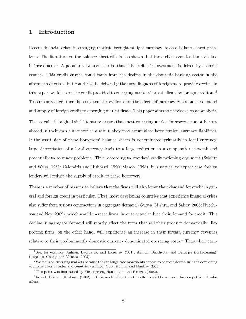
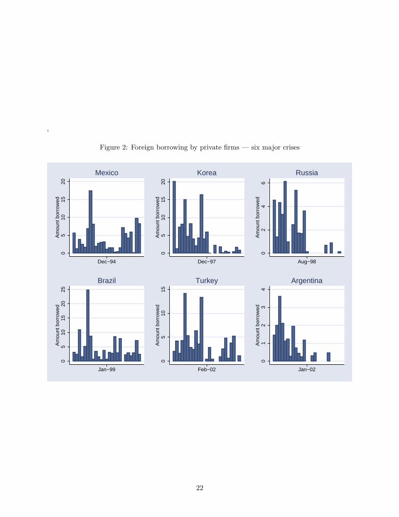
Table 2 summarize the amount borrowed by each sector in our sample.

We divide each amount by the US CPI to obtain the amount of credit for each sector–country–

month in real dollars. We then construct our dependent variables as a percentage deviation from

the country–specific average for each of the sectors.12 We do not exclude crisis periods from our

means, which biases the means downwards; therefore, the effects we find can be in practice larger.

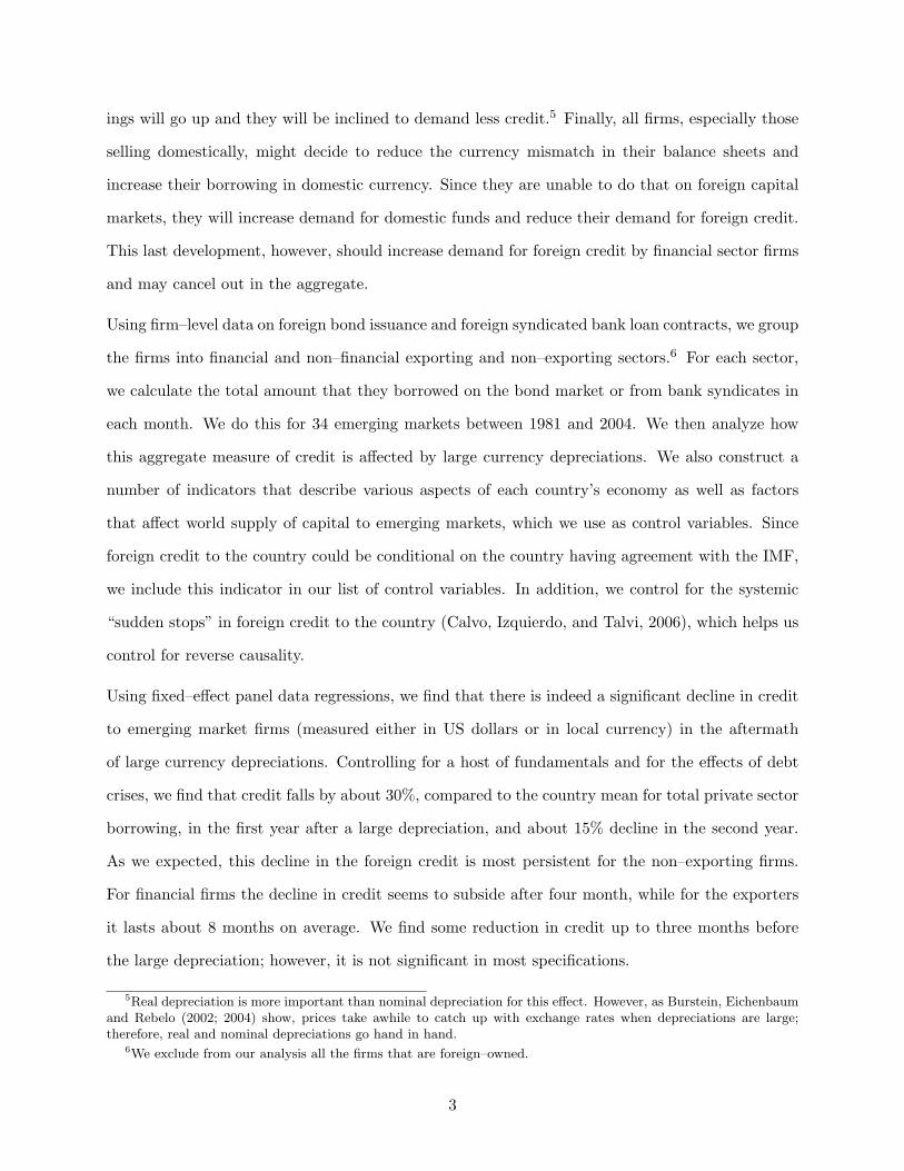
Figure 2 illustrates the dynamics of the credit for the six major currency crises of the 1990s.

2.5 Cost of credit: pit

In order to estimate demand and supply equations separately, we need a measure of a cost of

credit. Unfortunately, Loanware and Bondware do not provide sufficient information on the pricing

9Bond data start in March 1991, due to the fact that the bond market for emerging markets basically did notexist in the 1980s.

10Desai, Foley, and Forbes (2004) find that multinationals expand their activities and credit as a result of currencydepreciation.

11Table 3 presents sample industries in exporting and non–exporting sectors.12We use percentage deviations from the country–specific sample means for all continuous variables. Differences in

means are captured by country fixed effects, while common trends are captured by year fixed effects.

7

of credit. They include spreads only on a small subset of loan contracts and bond issues and

these spreads are only primary — there is no information on secondary market pricing of credit. In

addition, the pricing of each individual loan or bond issue might be driven by specific characteristics

of the firms borrowing in a particular month.

Secondary price data are available only for a small subset of the bonds and is also quite sparse. For

this reason, we resort to the JP Morgan country–specific EMBI Global Market Values Index. For

the cases when a country–specific index is not available, we use the region–specific index.13 We use

percentage deviations of the index from country–specific 10-year averages. This index represents

the price of country bonds on the secondary market; as such, it is inversely related to the cost of

credit. Thus, we expect the demand curve to have a positive slope with respect to this measure.

The EMBI Global indexes only go as far back as January 1994; therefore, our analysis of demand

and supply is limited to the 1994-2004 time period. However, we still capture the effects of currency

depreciation episodes that occurred up to two years prior to January 1994.

2.6 Demand and supply controls: Xdit

The control variables are indexes that describe different dimensions of the economy.14 In each case,

the variables are used as percentage deviation from their 25-year country–specific average from

1980 to 2004 on a monthly basis. All the indexes described below are lagged by one month.15

Since many of the variables we would like to control for are highly correlated, we construct the

indexes using the method of principal components. Because a principal component is a linear

combination of the variables that enter it, in cases when some variables are missing, other weights

can be re–scaled to compensate for missing variables. In this way, some of the gaps in the data

may be filled, which in our case of many missing observations is a main advantage of using these

indexes.

13We use the Africa index for Ghana; the Middle East index for Bahrain, Qatar, Saudi Arabia and United ArabEmirates; the Asia index for Hong Kong, India, Singapore and Taiwan; the ”Non-Latin” index for Czech Republic,Romania and Slovakia.

14We draw on the broad empirical literature on emerging market spreads to select our variables (Eichengreen, Hale,and Mody, 2001; Eichengreen and Mody, 2000b; Eichengreen and Mody, 2000a; Gelos, Sahay, and Sandleris, 2004;Kaminsky, Lizondo, and Reinhart, 1998; Mody, Taylor, and Kim, 2001).

15This turns out not to make much difference in our estimates compared to the case when they are not lagged.

8

We group the variables in the following categories, summarized in Table 4. For each of these

indexes, we use only the first principal component in our estimation.

• International competitiveness. A country’s international competitiveness affects the prof-

itability of firms in both the export and in import substitution sectors and therefore their

demand for credit. It also reflects a country’s ability to bring in enough foreign currency

to service its foreign debt and thus will affect foreign investors’ interest in the country. The

following variables are used to construct the index: terms of trade, change in current account,

change in real exchange rate,16 index of the market prices of the country’s export commodi-

ties,17 and volatility of export revenues. This index is scaled by a measure of trade openness

— the ratio of trade volume (sum of exports and imports) to GDP.

• Investment climate and monetary stability. This index accounts for the short–run

macroeconomic situation in the country. It reflects demand for investment, the availability

of domestic funds, and foreign investors’ interest in the country. This index is constructed

using the following variables: ratio of debt service to exports, ratio of investment to GDP,

real interest rate, ratio of lending interest rate to deposit interest rate, inflation rate, ratio of

domestic credit to GDP, and change in the domestic stock market index.

• Financial development. The level of development of the financial market affects domestic

funding opportunities for firms and, therefore, their demand for foreign credit. This index is

based on the ratio of stock market capitalization to GDP, the ratio of commercial bank assets

to GDP, and the degree of financial account openness, which reflects how easy it is for firms

to access foreign capital directly.

• Long–run macroeconomic prospects. The economy’s growth prospects affect the invest-

ment demand of firms. This index is based on the ratio of total foreign debt to GDP, the

16Nominal exchange rates were obtained from various data sources. For countries that changed the denominationof their currency, continuous series were constructed to reflect true changes in currency values.

17Many emerging markets rely heavily on the export of a small number of commodities. We identify up to five ofthese commodities (or commodity groups) for each country and merge these data with monthly commodity pricesfrom the Global Financial Data and the International Financial Statistics. For each commodity, we calculate monthlypercentage deviations from its 25-year average (1980-2004). For each country and each month, we construct the indexas a simple average of relevant deviations of commodity prices. If a country is exporting a variety of manufacturedgoods and does not rely on commodity exports, this index is set to zero.

9

growth rate of real GDP, the growth rate of nominal GDP measured in US dollars, and the

unemployment rate.

In addition to the indexes we include indicators for the sovereign debt crises as defined by Arteta

and Hale (2006), since sovereign debt crises are found to affect both demand and supply of credit.

2.7 Supply controls: Xsit

The following variables are included in the reduced form equation and in the supply (price) equation.

We believe that they do not directly affect the demand for foreign funds by emerging market private

borrowers.

Global supply of capital. This index reflects the availability of capital in general, changes in

investors’ risk attitude, and their willingness to provide capital to emerging markets. This index is

constructed on the basis of an investor confidence index, the growth rate of the US stock market in-

dex, the US Treasury rate, the volume of gross international capital outflows from OECD countries,

and Merrill Lynch High Yield Spreads. All variables are presented as percentage deviations from

their 25–year average. Two principal components are retained and capture 65% of the variance.

This index is not country–specific and therefore does not affect an individual country’s changes in

its demand for credit.

We include two more variables: a dummy variable indicating whether the country has an IMF

agreement in place, and a dummy variable indicating whether the country experience an influence

of a “systemic sudden stop” in capital inflows in a given month.

Some creditors are not able or willing to lend to the countries that do not have an IMF agreement

in place; therefore, the supply of credit to these countries can be adversely affected, especially in

the aftermath of sovereign default. We set this variable equal to one if either a stand–by or an

extended funds facility is in place for each month for a given country. Since the IMF funding is

extended to sovereigns, they might affect sovereign demand for funds from commercial creditors,

but are not likely to directly affect private demand for foreign credit.

Calvo (1998) argues that capital flows to a country could dry up for reasons not completely in

10

control of the country. If an exogenous “sudden stop” in capital flows occurs, it is likely to cause

both currency depreciation and a decline in foreign credit, thus potentially creating a spurious

relationship between currency depreciation and supply of credit. Thus, we want to control for

these sudden stops. Since these sudden stops would not necessarily occur in all countries, and

therefore they would not be captured by our measure of the global supply of capital. Thus, we

include an indicator that is equal to one in each month a given country was affected by a systemic

sudden stop in capital inflows, according to Calvo, Izquierdo, and Talvi (2006). Where this variable

is missing, we supplement it with the annual sudden stop indicator from Frankel and Cavallo (2004).

3 Empirical findings

We first analyze whether there is a reduction in credit due to large currency depreciations and then

analyze demand and supply effects separately. We first focus on the long run — including our main

explanatory variable for up to two years. We then repeat the analysis with monthly indicators of

the event. The coefficients in the regressions are easy to interpret: Since the dependent variable

(amount of credit) is defined as a percentage deviation from the mean, the coefficients on binary

variables indicate the percentage change (relative to the mean) of the dependent variable if the

indicator value switches from 0 to 1.

3.1 Reduced form

The results for the reduced form analysis that tests for a decline in credit in the aftermath of a

currency depreciation are presented in Tables 5 through 7.

In Table 5, the dependent variable is the percentage deviation in the foreign credit received by

the entire private sector. The first three columns present the results that are obtained without

including any of the control variables described in the previous section. We can see that, if we do

not control for fundamentals, the decline in credit after large currency depreciation events is large

— over 30% in the first two years after the even. This effect remains even if we control for country

and year fixed effects.

11

The last three columns include additional control variables (fundamentals). We can see that the

effect of depreciation is now smaller (i.e., some decline we observed in first three columns is due

to worsening fundamentals); however, it remains significant. The magnitude of the decline is now

between 25% and 30% in the first year, and just over 20% in the second year after depreciation.18

The second year effect declines further if we control for the effects of sovereign debt re–negotiations

and rescheduling as defined in Arteta and Hale (2006): in column (6) it is 16%, which is still rather

large.

Table 6 repeats this analysis for the percentage deviation in the credit obtained by the private

sector measured in local currency, rather than in US dollars, as in Table 5. Since most firms’ costs

are denominated in local currency, it would be natural to expect a decline in demand for foreign

currency credit after a large depreciation of the currency. Since most borrowing occurs in the

foreign currency, we translate borrowing into local currency using the average exchange rate for

each month, and then correct the measure by the local CPI.19 The effects we find are very similar

to the ones obtained with the credit measured in dollars. Thus, we are confident that we find an

actual decline in credit rather than a mere accounting readjustment due to changes in the currency

values. Since the local currency measure is very noisy, we proceed with US dollar measures.

In Table 7 we present the results of our analysis by sector, using the specification of column (6)

in Table 5. The dependent variable in each regression is the percentage change in the amount of

credit extended to each sector. We find that financial sector experiences a large decline in credit in

the month of the crisis, but that the effect of depreciation is less persistent than for non–financial

sector (compare columns (1) and (2)). Among non–financial firms, we find that the effect is more

persistent for the non–exporting firms. In fact, the non–exporting sector is the only sector for which

the effect lasts more than a year.

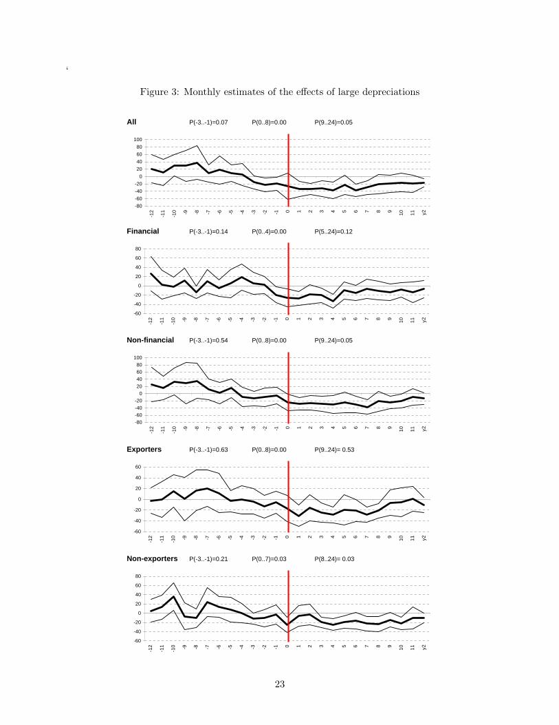
In order to analyze how fast the effect of depreciations wears out, we re–estimate regressions in

Table 7 with monthly rather than annual dummy variables for the lagged effects of depreciations.

We also include up to 12 months leads to control for simultaneity and expected currency crises.

18One must note that the differences in coefficients across specifications are not statistically significant.19Prices tend to adjust quite slowly after large depreciation events (Burstein, Eichenbaum, and Rebelo, 2002;

Burstein, Eichenbaum, and Rebelo, 2004), thus our “real local currency” measure of credit is quite different from theone measured in dollars.

12

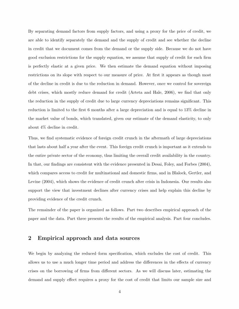
The estimates and their confidence intervals are presented on Figure 3. We can see that for the

private sector as a whole, the decline in credit seems to last for two years, which is confirmed by

the F–test, presented above the graph. However, as we have established in Table 7, this effect is

driven entirely by non–exporting firms. The financial sector seems to recover its access to credit 4

months after the depreciation, and exporting firms 8 months after the depreciation. These results

are expected — financial firms are more likely to have closer ties with their lenders in general and

therefore be less credit constrained, while exporters are less likely to experience the balance–sheet

effects of depreciation that firms selling domestically would experience.

Note that for the private sector as a whole, the decline in credit appears to start about 3 months

before the actual depreciation. This can represent some simultaneity effect of capital flow reversals,

that would lead to both decline in credit and currency depreciation. However, since we do control

for the sudden stops and given that for each sector this decline is not significant, it is more likely

that some depreciation events were expected, as would be in the case of the collapse of a fixed

exchange rate regime as in Argentina in 2001.20

3.2 Demand and supply effects

We now turn to demand and supply effects. Since we discovered that there is some decline in

credit in the three months prior to currency depreciation, we include an indicator for three months

before the event. In addition, we split the effects of the first year into two half–year indicators, in

order to analyze how fast the effects subside. The results are presented in Table 8. The number of

observations is smaller due to the fact that price data only go back to 1994.

First we note, reassuringly, that the coefficient on the price in the demand equation (labeled

”Amount”) is positive and significant. Since the price is measure as a market value of the debt,

it is the inverse of the cost of credit, and therefore we would expect the demand for credit to

positively depend on the market value of debt. Our estimated elasticity of demand suggests that

a 10% increase in the market value of the debt would increase the demand for credit by 3% on

average.

20We will allow for the leads in our analysis of demand and supply effect and will see that there is no significantdecline in the supply of credit prior to currency depreciation.

13

In Model 1, presented in columns (1) and (2), the supply equation does not include the controls

for fundamentals. As column (1) shows, we observe a large decline in the market value of the debt

that persists for a full year. However, once we control for fundamentals (Model 2, column(3)), we

find that a reduction in the supply of credit was largely due to the decline in fundamentals. The

leftover effect only lasts six months and is now much smaller.

In both Model 1 and 2, we observe a dramatic decline in the demand for credit, on the order

45% in the first six months after a currency depreciation. However, once we include the indicators

for sovereign debt crises (Model 3), we find that the decline in demand, while still sizable (the

magnitude is about 20%), is no longer statistically significant. We still find a decline in supply

during first six months after depreciation, of almost 13%. While this represents a rather sizable

decline in the value of debt, it only translates in to a 4% decline in credit, given our estimated

demand elasticity.

Even though the estimated effects of currency depreciation on the demand for credit are not sta-

tistically significant, we know that demand has to contribute to the total decline in credit, given

the results of our reduced form analysis. However, since the estimates are very noisy (possibly due

to a much smaller sample size), we cannot make definitive statements regarding the size of these

effects.

Thus, we can conclude from this section that we indeed observe a credit crunch in the aftermath

of currency crises, or large depreciation episodes in general, which is consistent with the view that

balance sheets worsen due to currency depreciation. This finding provides a potential explanation

for the decline in investment associated with currency crises.

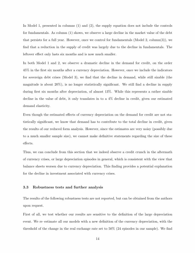
3.3 Robustness tests and further analysis

The results of the following robustness tests are not reported, but can be obtained from the authors

upon request.

First of all, we test whether our results are sensitive to the definition of the large depreciation

event. We re–estimate all our models with a new definition of the currency depreciation, with the

threshold of the change in the real exchange rate set to 50% (24 episodes in our sample). We find

14

that, while the effects of these larger currency depreciation events are larger (40% decline in the

reduced form) and and more persistent (credit crunch of 10-12% lasts about 2 years), the basic

message of the paper remains unchanged.

We re–estimate our model replacing the large depreciation indicators with a continuous variable

that measures percentage change in the nominal exchange rate in each month. We find no significant

effects of this variable, whether contemporaneous or lagged, in a robust form specification, which

suggests that our results are indeed driven by large depreciations. We do find a negative coefficient

on a 1-month lagged change in real exchange rate, which is significant at 8% level. This finding is

consistent with our results on the credit crunch.

We re–estimate our model separating depreciation episodes that were devaluations or switches from

pre–announced peg to floating regime from those which were depreciations under float. We find

that the decline in credit occurs in both cases, but is larger in case of a regime switch.

To see whether our results are driven entirely by the 1980s, we re–estimate the regressions in Table

5 splitting the sample into 1980-1989 the 1990-2004 time periods. We find that the decline in credit

in the 1980s (31 episodes of currency depreciation) was about 16% and only lasted one year, while

the decline in the 1990s (38 episodes) was about 36% in the first year and 20% in the second year.21

We re–estimated our model adding 12 month fixed effects to control for any possible seasonality.

While we find that credit in months of January and February tends to be lower, this effect does

not change our results at all.

When the political situation in a country is unstable, it introduces uncertainty and leads to a decline

in firms’ investment and their demand for credit; furthermore, it may lead to foreign investors’

concerns about their ability to collect their assets in the future. We used the measure of political risk

from the International Country Risk Guide (ICRG). While this index does enter significantly with

the correct sign in most regressions, it does not affect our qualitative or quantitative conclusions.

It does limit our simple size and therefore reduces the significance level of some coefficients.

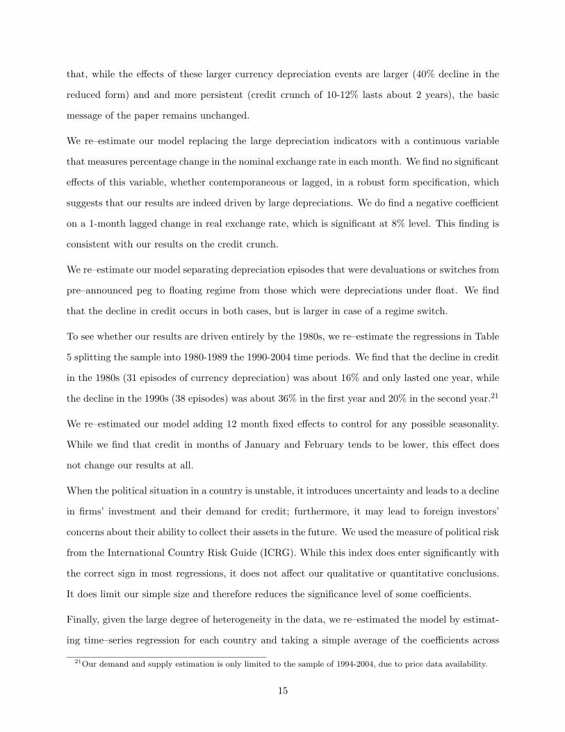
Finally, given the large degree of heterogeneity in the data, we re–estimated the model by estimat-

ing time–series regression for each country and taking a simple average of the coefficients across

21Our demand and supply estimation is only limited to the sample of 1994-2004, due to price data availability.

15

countries. The coefficients of interest obtained in this manner are very close to those we estimate

in our fixed effects specifications, thus confirming that the effects we find are indeed systematic and

robust.

4 Conclusion

We analyze a data set built on the firm–level data in order to examine the effects of large currency

depreciations on the foreign credit to the private sector. Controlling for fundamentals and the

effects of sovereign debt crises, we find that foreign credit to the private sector declines by about

30% overall and that non–financial non–exporting sector firms are hit the most, in the sense that

the decline of credit to this sector is very persistent.

We find that both demand and supply take a hit after the large depreciations. However, only the

decline in supply is statistically significant, and only in first six months after currency depreciation.

These results and the results of the reduced form analysis are consistent with the view that currency

crises lead to the balance sheet effects that in turn can worsen credit rationing.

These results are in contrast to the findings in Arteta and Hale (2006), which shows that a decline

in credit to private sector as a result of sovereign debt crisis is mostly due to a decline in demand

for credit (results that we confirm but not emphasize in this paper).

16

References

Aghion, P., P. Bacchetta, and A. Banerjee (2001): “Currency crises and monetary policy

in an economy with credit constraints,” European Economic Review, 45(7), 1121–1150.

(forthcoming): “A Corporate Balance-Sheet Approach to Currency Crises,” Journal of

Economic Theory, 45(7), 1121–1150.

Ahmed, S., C. J. Gust, S. B. Kamin, and J. Huntley (2002): “Are depreciations as con-

tractionary as devaluations? A comparison of selected emerging and industrial economies,”

International Finance Discussion Papers 737, Board of Governors of the Federal Reserve System

(U.S.).

Arteta, C., and G. Hale (2006): “Are Private Borrowers Hurt by Sovereign Debt Reschedul-

ing?,” mimeo, Yale University.

Blalock, G., P. J. Gertler, and D. I. Levine (2004): “Investment Following a Financial

Crisis: Does Foreign Ownership Matter?,” Paper presented at SCCIE workshop on “Firms in

Emerging Markets” May 20, 2005.

Bris, A., and Y. Koskinen (2002): “Corporate Leverage and Currency Crises,” Journal of

Financial Economics, 63(2), 275–331.

Burstein, A. T., M. Eichenbaum, and S. T. Rebelo (2002): “Why Are Rates of Inflation So

Low After Large Devaluations?,” NBER Working Paper No. W8748.

Burstein, A. T., M. Eichenbaum, and S. T. Rebelo (2004): “Large Devaluations and the

Real Exchange Rate,” NBER Working Paper No. W10986.

Calomiris, C. W., and R. G. Hubbard (1990): “Firm Heterogeneity, International Finance,

and ‘Credit Rationing’,” The Economic Journal, 100(399), 90–104.

Calvo, G. (1998): “Capital Flows and Capital Market Crises: The Simple Economics of Sudden

Stops,” Journal of Applied Economics, 1, 35–54.

17

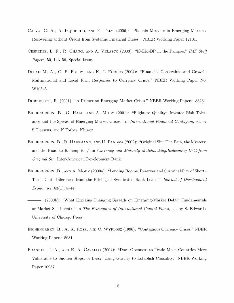
Calvo, G. A., A. Izquierdo, and E. Talvi (2006): “Phoenix Miracles in Emerging Markets:

Recovering without Credit from Systemic Financial Crises,” NBER Working Paper 12101.

Cespedes, L. F., R. Chang, and A. Velasco (2003): “IS-LM-BP in the Pampas,” IMF Staff

Papers, 50, 143–56, Special Issue.

Desai, M. A., C. F. Foley, and K. J. Forbes (2004): “Financial Constraints and Growth:

Multinational and Local Firm Responses to Currency Crises,” NBER Working Paper No.

W10545.

Dornbusch, R. (2001): “A Primer on Emerging Market Crises,” NBER Working Papers: 8326.

Eichengreen, B., G. Hale, and A. Mody (2001): “Flight to Quality: Investor Risk Toler-

ance and the Spread of Emerging Market Crises,” in International Financial Contagion, ed. by

S.Classens, and K.Forbes. Kluwer.

Eichengreen, B., R. Hausmann, and U. Panizza (2002): “Original Sin: The Pain, the Mystery,

and the Road to Redemption,” in Currency and Maturity Matchmaking:Redeeming Debt from

Original Sin. Inter-American Development Bank.

Eichengreen, B., and A. Mody (2000a): “Lending Booms, Reserves and Sustainability of Short–

Term Debt: Inferences from the Pricing of Syndicated Bank Loans,” Journal of Development

Economics, 63(1), 5–44.

(2000b): “What Explains Changing Spreads on Emerging-Market Debt? Fundamentals

or Market Sentiment?,” in The Economics of International Capital Flows, ed. by S. Edwards.

University of Chicago Press.

Eichengreen, B., A. K. Rose, and C. Wyplosz (1996): “Contagious Currency Crises,” NBER

Working Papers: 5681.

Frankel, J. A., and E. A. Cavallo (2004): “Does Openness to Trade Make Countries More

Vulnerable to Sudden Stops, or Less? Using Gravity to Establish Causality,” NBER Working

Paper 10957.

18

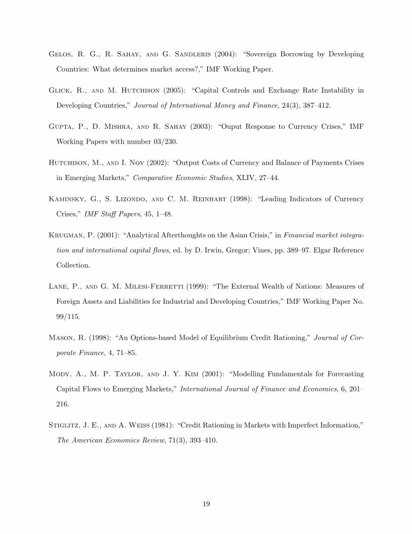
Gelos, R. G., R. Sahay, and G. Sandleris (2004): “Sovereign Borrowing by Developing

Countries: What determines market access?,” IMF Working Paper.

Glick, R., and M. Hutchison (2005): “Capital Controls and Exchange Rate Instability in

Developing Countries,” Journal of International Money and Finance, 24(3), 387–412.

Gupta, P., D. Mishra, and R. Sahay (2003): “Ouput Response to Currency Crises,” IMF

Working Papers with number 03/230.

Hutchison, M., and I. Noy (2002): “Output Costs of Currency and Balance of Payments Crises

in Emerging Markets,” Comparative Economic Studies, XLIV, 27–44.

Kaminsky, G., S. Lizondo, and C. M. Reinhart (1998): “Leading Indicators of Currency

Crises,” IMF Staff Papers, 45, 1–48.

Krugman, P. (2001): “Analytical Afterthoughts on the Asian Crisis,” in Financial market integra-

tion and international capital flows, ed. by D. Irwin, Gregor; Vines, pp. 389–97. Elgar Reference

Collection.

Lane, P., and G. M. Milesi-Ferretti (1999): “The External Wealth of Nations: Measures of

Foreign Assets and Liabilities for Industrial and Developing Countries,” IMF Working Paper No.

99/115.

Mason, R. (1998): “An Options-based Model of Equilibrium Credit Rationing,” Journal of Cor-

porate Finance, 4, 71–85.

Mody, A., M. P. Taylor, and J. Y. Kim (2001): “Modelling Fundamentals for Forecasting

Capital Flows to Emerging Markets,” International Journal of Finance and Economics, 6, 201–

216.

Stiglitz, J. E., and A. Weiss (1981): “Credit Rationing in Markets with Imperfect Information,”

The American Economics Review, 71(3), 393–410.

19

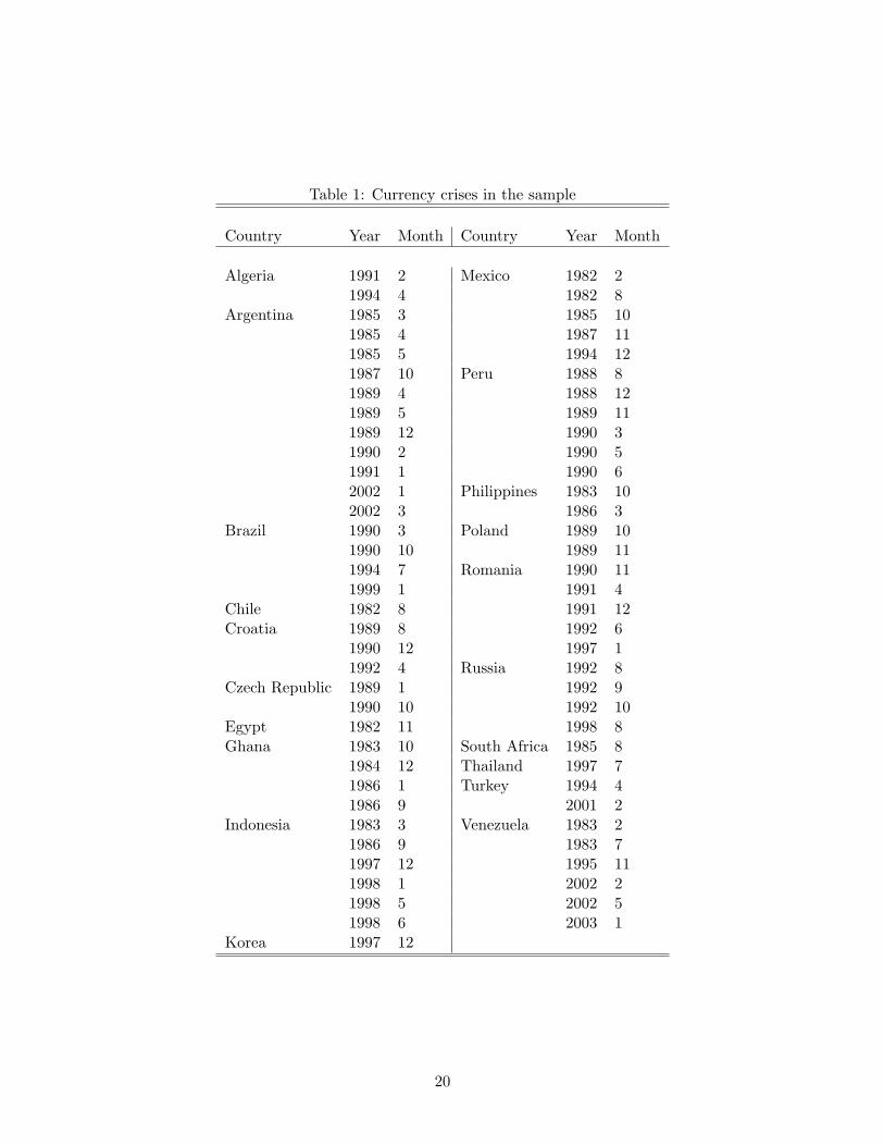
Table 1: Currency crises in the sample

Country Year Month Country Year Month

Algeria 1991 2 Mexico 1982 21994 4 1982 8

Argentina 1985 3 1985 101985 4 1987 111985 5 1994 121987 10 Peru 1988 81989 4 1988 121989 5 1989 111989 12 1990 31990 2 1990 51991 1 1990 62002 1 Philippines 1983 102002 3 1986 3

Brazil 1990 3 Poland 1989 101990 10 1989 111994 7 Romania 1990 111999 1 1991 4

Chile 1982 8 1991 12Croatia 1989 8 1992 6

1990 12 1997 11992 4 Russia 1992 8

Czech Republic 1989 1 1992 91990 10 1992 10

Egypt 1982 11 1998 8Ghana 1983 10 South Africa 1985 8

1984 12 Thailand 1997 71986 1 Turkey 1994 41986 9 2001 2

Indonesia 1983 3 Venezuela 1983 21986 9 1983 71997 12 1995 111998 1 2002 21998 5 2002 51998 6 2003 1

Korea 1997 12

20

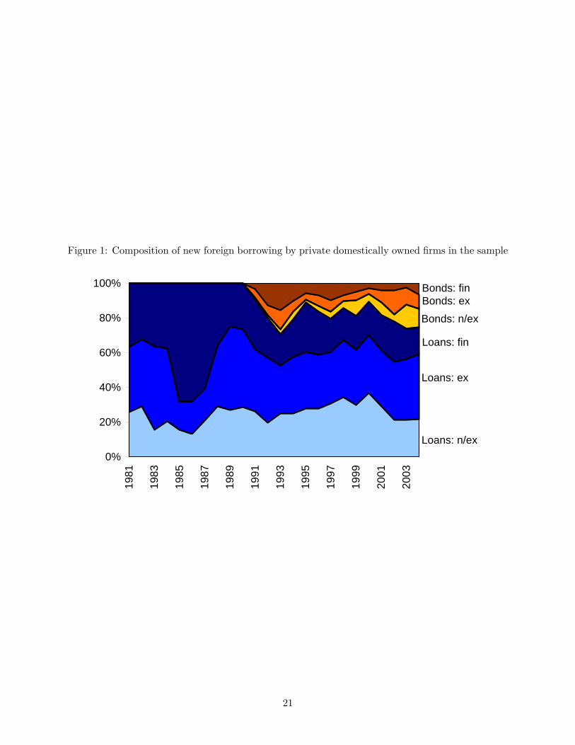
Figure 1: Composition of new foreign borrowing by private domestically owned firms in the sampleComposition of foreign borrowing by private domestically owned firms (in the sample)

0%

20%

40%

60%

80%

100%

1981

1983

1985

1987

1989

1991

1993

1995

1997

1999

2001

2003

Loans: n/ex

Loans: ex

Loans: fin

Bonds: n/exBonds: exBonds: fin

21

‘

Figure 2: Foreign borrowing by private firms — six major crises

05

1015

20A

mou

nt b

orro

wed

Dec−94

Mexico0

510

1520

Am

ount

bor

row

ed

Dec−97

Korea

02

46

Am

ount

bor

row

edAug−98

Russia

05

1015

2025

Am

ount

bor

row

ed

Jan−99

Brazil

05

1015

Am

ount

bor

row

ed

Feb−02

Turkey

01

23

4A

mou

nt b

orro

wed

Jan−02

Argentina

22

‘

Figure 3: Monthly estimates of the effects of large depreciations

All P(-3..-1)=0.07 P(0..8)=0.00 P(9..24)=0.05

Financial P(-3..-1)=0.14 P(0..4)=0.00 P(5..24)=0.12

Non-financial P(-3..-1)=0.54 P(0..8)=0.00 P(9..24)=0.05

Exporters P(-3..-1)=0.63 P(0..8)=0.00 P(9..24)= 0.53

Non-exporters P(-3..-1)=0.21 P(0..7)=0.03 P(8..24)= 0.03

-80-60-40-20

020406080

100

-12

-11

-10 -9 -8 -7 -6 -5 -4 -3 -2 -1 0 1 2 3 4 5 6 7 8 9 10 11 y2

-60

-40

-20

0

20

40

60

80

-12

-11

-10 -9 -8 -7 -6 -5 -4 -3 -2 -1 0 1 2 3 4 5 6 7 8 9 10 11 y2

-80-60-40-20

020406080

100

-12

-11

-10 -9 -8 -7 -6 -5 -4 -3 -2 -1 0 1 2 3 4 5 6 7 8 9 10 11 y2

-60

-40

-20

0

20

40

60

-12

-11

-10 -9 -8 -7 -6 -5 -4 -3 -2 -1 0 1 2 3 4 5 6 7 8 9 10 11 y2

-60

-40

-20

0

20

40

60

80

-12

-11

-10 -9 -8 -7 -6 -5 -4 -3 -2 -1 0 1 2 3 4 5 6 7 8 9 10 11 y2

23

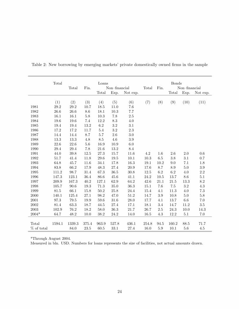
Table 2: New borrowing by emerging markets’ private domestically owned firms in the sample

Total Loans BondsTotal Fin. Non–financial Total Fin. Non–financial

Total Exp. Not exp. Total Exp. Not exp.

(1) (2) (3) (4) (5) (6) (7) (8) (9) (10) (11)1981 29.2 29.2 10.7 18.5 11.0 7.61982 26.6 26.6 8.6 18.1 10.3 7.71983 16.1 16.1 5.8 10.3 7.8 2.51984 19.6 19.6 7.4 12.2 8.3 4.01985 19.4 19.4 13.2 6.2 3.2 3.11986 17.2 17.2 11.7 5.4 3.2 2.31987 14.4 14.4 8.7 5.7 2.6 3.01988 13.3 13.3 4.8 8.5 4.6 3.91989 22.6 22.6 5.6 16.9 10.9 6.01990 29.4 29.4 7.8 21.6 13.2 8.41991 44.0 39.8 12.5 27.3 15.7 11.6 4.2 1.6 2.6 2.0 0.61992 51.7 41.4 11.8 29.6 19.5 10.1 10.3 6.5 3.8 3.1 0.71993 64.8 45.7 11.6 34.1 17.8 16.3 19.1 10.2 9.0 7.1 1.81994 83.8 66.2 17.9 48.3 27.4 20.9 17.6 8.7 8.9 5.0 3.91995 111.2 98.7 31.4 67.3 36.5 30.8 12.5 6.2 6.2 4.0 2.21996 147.3 123.1 36.4 86.6 45.6 41.1 24.2 10.5 13.7 8.6 5.11997 209.9 167.3 40.2 127.1 62.9 64.2 42.6 21.1 21.5 13.3 8.21998 105.7 90.6 19.3 71.3 35.0 36.3 15.1 7.6 7.5 3.2 4.31999 81.5 66.1 15.8 50.2 25.8 24.4 15.4 4.1 11.3 4.0 7.32000 140.1 125.4 27.1 98.2 47.0 51.2 14.7 3.9 10.8 5.0 5.82001 97.3 79.5 19.9 59.6 31.6 28.0 17.7 4.1 13.7 6.6 7.02002 81.4 63.3 18.7 44.5 27.4 17.1 18.1 3.4 14.7 11.2 3.52003 102.9 76.2 18.2 58.0 36.3 21.7 26.7 2.5 24.3 10.0 14.32004* 64.7 48.2 10.0 38.2 24.2 14.0 16.5 4.3 12.2 5.1 7.0

Total 1594.1 1339.3 375.4 963.9 527.8 436.1 254.8 94.5 160.2 88.5 71.7% of total 84.0 23.5 60.5 33.1 27.4 16.0 5.9 10.1 5.6 4.5

*Through August 2004.Measured in bln. USD. Numbers for loans represents the size of facilities, not actual amounts drawn.

24

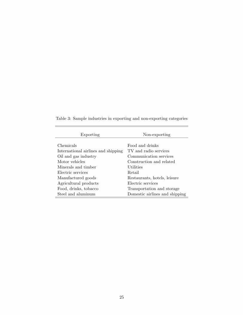
Table 3: Sample industries in exporting and non-exporting categories

Exporting Non-exporting

Chemicals Food and drinksInternational airlines and shipping TV and radio servicesOil and gas industry Communication servicesMotor vehicles Construction and relatedMinerals and timber UtilitiesElectric services RetailManufactured goods Restaurants, hotels, leisureAgricultural products Electric servicesFood, drinks, tobacco Transportation and storageSteel and aluminum Domestic airlines and shipping

25

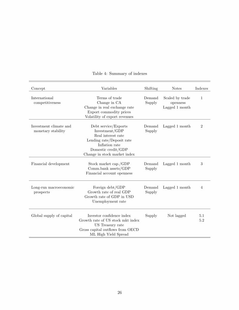
Table 4: Summary of indexes

Concept Variables Shifting Notes Indexes

International Terms of trade Demand Scaled by trade 1competitiveness Change in CA Supply openness

Change in real exchange rate Lagged 1 monthExport commodity prices

Volatility of export revenues

Investment climate and Debt service/Exports Demand Lagged 1 month 2monetary stability Investment/GDP Supply

Real interest rateLending rate/Deposit rate

Inflation rateDomestic credit/GDP

Change in stock market index

Financial development Stock market cap./GDP Demand Lagged 1 month 3Comm.bank assets/GDP Supply

Financial account openness

Long-run macroeconomic Foreign debt/GDP Demand Lagged 1 month 4prospects Growth rate of real GDP Supply

Growth rate of GDP in USDUnemployment rate

Global supply of capital Investor confidence index Supply Not lagged 5.1Growth rate of US stock mkt index 5.2

US Treasury rateGross capital outflows from OECD

ML High Yield Spread

26

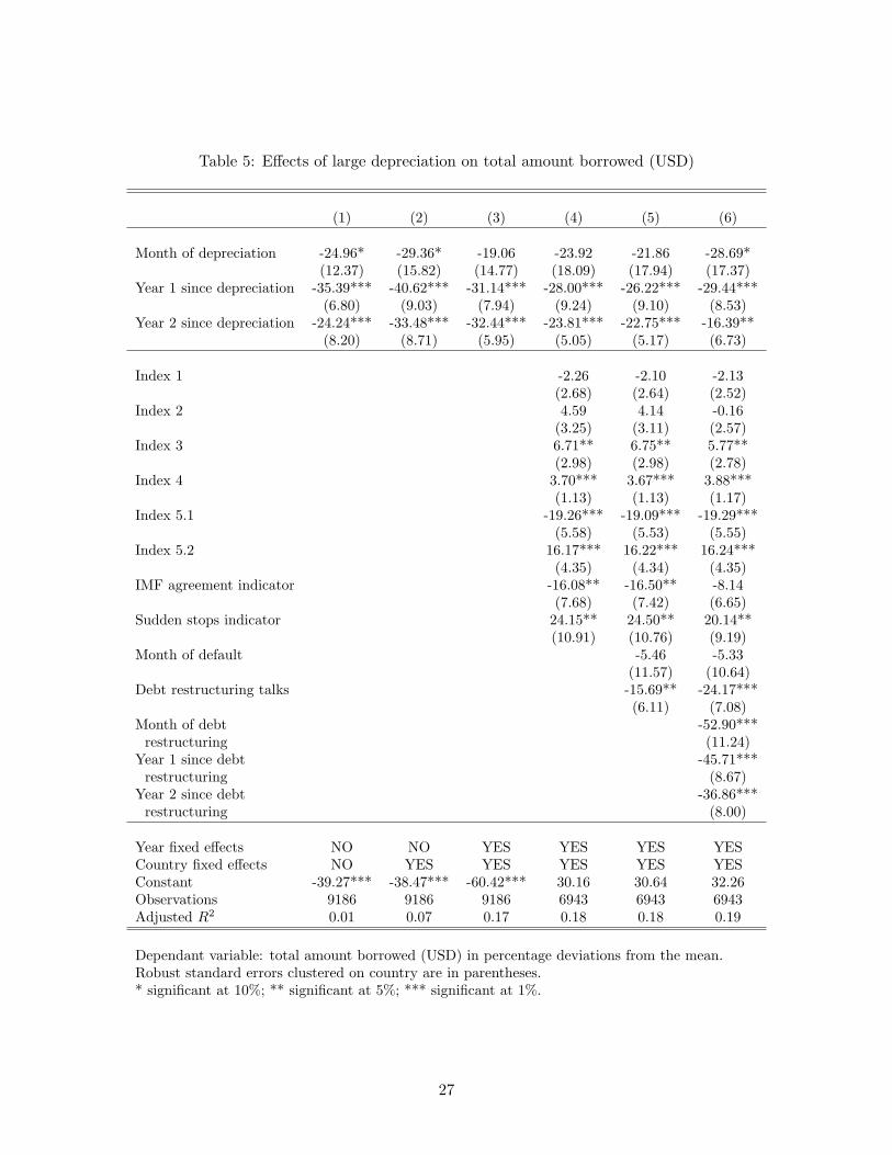
Table 5: Effects of large depreciation on total amount borrowed (USD)

(1) (2) (3) (4) (5) (6)

Month of depreciation -24.96* -29.36* -19.06 -23.92 -21.86 -28.69*(12.37) (15.82) (14.77) (18.09) (17.94) (17.37)

Year 1 since depreciation -35.39*** -40.62*** -31.14*** -28.00*** -26.22*** -29.44***(6.80) (9.03) (7.94) (9.24) (9.10) (8.53)

Year 2 since depreciation -24.24*** -33.48*** -32.44*** -23.81*** -22.75*** -16.39**(8.20) (8.71) (5.95) (5.05) (5.17) (6.73)

Index 1 -2.26 -2.10 -2.13(2.68) (2.64) (2.52)

Index 2 4.59 4.14 -0.16(3.25) (3.11) (2.57)

Index 3 6.71** 6.75** 5.77**(2.98) (2.98) (2.78)

Index 4 3.70*** 3.67*** 3.88***(1.13) (1.13) (1.17)

Index 5.1 -19.26*** -19.09*** -19.29***(5.58) (5.53) (5.55)

Index 5.2 16.17*** 16.22*** 16.24***(4.35) (4.34) (4.35)

IMF agreement indicator -16.08** -16.50** -8.14(7.68) (7.42) (6.65)

Sudden stops indicator 24.15** 24.50** 20.14**(10.91) (10.76) (9.19)

Month of default -5.46 -5.33(11.57) (10.64)

Debt restructuring talks -15.69** -24.17***(6.11) (7.08)

Month of debt -52.90***restructuring (11.24)

Year 1 since debt -45.71***restructuring (8.67)

Year 2 since debt -36.86***restructuring (8.00)

Year fixed effects NO NO YES YES YES YESCountry fixed effects NO YES YES YES YES YESConstant -39.27*** -38.47*** -60.42*** 30.16 30.64 32.26Observations 9186 9186 9186 6943 6943 6943Adjusted R2 0.01 0.07 0.17 0.18 0.18 0.19

Dependant variable: total amount borrowed (USD) in percentage deviations from the mean.Robust standard errors clustered on country are in parentheses.* significant at 10%; ** significant at 5%; *** significant at 1%.

27

Table 6: Effects of large depreciation on total amount borrowed (local currency)

(1) (2) (3) (4) (5) (6)

Month of depreciation -52.10*** -65.80*** -36.25** -26.73* -26.75* -33.11**(11.93) (17.25) (15.88) (15.89) (15.22) (14.71)

Year 1 since depreciation -54.40*** -65.39*** -36.37*** -23.73* -21.94* -25.00*(8.65) (13.07) (12.65) (13.03) (13.10) (12.96)

Year 2 since depreciation -45.67*** -59.63*** -41.01*** -25.56* -24.74* -17.59(8.85) (11.24) (12.08) (13.19) (13.19) (15.92)

Index 1 1.71 1.78 1.86(3.18) (3.13) (2.83)

Index 2 7.17* 6.85* 2.61(3.74) (3.70) (3.39)

Index 3 4.20 4.24 3.23(3.40) (3.40) (3.34)

Index 4 4.93*** 4.92*** 5.00***(1.53) (1.50) (1.62)

Index 5.1 -26.92*** -26.92*** -27.33***(9.35) (9.37) (9.47)

Index 5.2 23.36*** 23.31*** 23.28***(6.61) (6.61) (6.66)

IMF agreement indicator -20.42** -20.71** -12.35(8.85) (8.66) (7.94)

Sudden stops indicator 22.81 23.42 18.97(14.98) (14.84) (13.28)

Month of default 29.10 30.81(26.93) (26.30)

Debt rescheduling talks -15.58** -23.88***(7.74) (8.01)

Month of debt -50.44***rescheduling (13.10)

Year 1 since debt -45.30***rescheduling (12.00)

Year 2 since debt -50.59***rescheduling (10.67)

Year fixed effects NO NO YES YES YES YESCountry fixed effects NO YES YES YES YES YESConstant -16.50*** -14.77*** -68.88*** 46.73 46.32 47.93Observations 7759 7759 7759 6536 6536 6536Adjusted R2 0.01 0.04 0.11 0.12 0.12 0.13

Dependant variable: total amount borrowed (local cur.) in percentage deviations from the mean.Robust standard errors clustered on country are in parentheses.* significant at 10%; ** significant at 5%; *** significant at 1%.

28

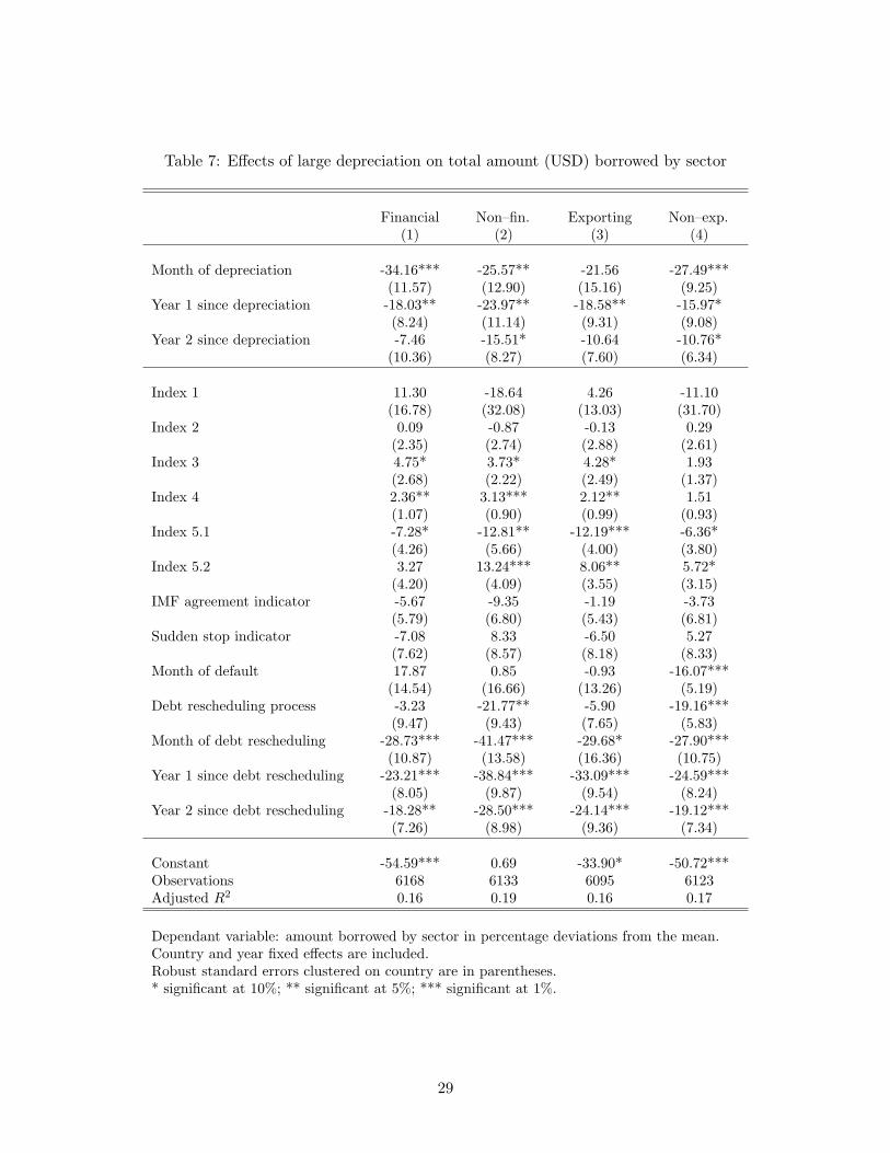
Table 7: Effects of large depreciation on total amount (USD) borrowed by sector

Financial Non–fin. Exporting Non–exp.(1) (2) (3) (4)

Month of depreciation -34.16*** -25.57** -21.56 -27.49***(11.57) (12.90) (15.16) (9.25)

Year 1 since depreciation -18.03** -23.97** -18.58** -15.97*(8.24) (11.14) (9.31) (9.08)

Year 2 since depreciation -7.46 -15.51* -10.64 -10.76*(10.36) (8.27) (7.60) (6.34)

Index 1 11.30 -18.64 4.26 -11.10(16.78) (32.08) (13.03) (31.70)

Index 2 0.09 -0.87 -0.13 0.29(2.35) (2.74) (2.88) (2.61)

Index 3 4.75* 3.73* 4.28* 1.93(2.68) (2.22) (2.49) (1.37)

Index 4 2.36** 3.13*** 2.12** 1.51(1.07) (0.90) (0.99) (0.93)

Index 5.1 -7.28* -12.81** -12.19*** -6.36*(4.26) (5.66) (4.00) (3.80)

Index 5.2 3.27 13.24*** 8.06** 5.72*(4.20) (4.09) (3.55) (3.15)

IMF agreement indicator -5.67 -9.35 -1.19 -3.73(5.79) (6.80) (5.43) (6.81)

Sudden stop indicator -7.08 8.33 -6.50 5.27(7.62) (8.57) (8.18) (8.33)

Month of default 17.87 0.85 -0.93 -16.07***(14.54) (16.66) (13.26) (5.19)

Debt rescheduling process -3.23 -21.77** -5.90 -19.16***(9.47) (9.43) (7.65) (5.83)

Month of debt rescheduling -28.73*** -41.47*** -29.68* -27.90***(10.87) (13.58) (16.36) (10.75)

Year 1 since debt rescheduling -23.21*** -38.84*** -33.09*** -24.59***(8.05) (9.87) (9.54) (8.24)

Year 2 since debt rescheduling -18.28** -28.50*** -24.14*** -19.12***(7.26) (8.98) (9.36) (7.34)

Constant -54.59*** 0.69 -33.90* -50.72***Observations 6168 6133 6095 6123Adjusted R2 0.16 0.19 0.16 0.17

Dependant variable: amount borrowed by sector in percentage deviations from the mean.Country and year fixed effects are included.Robust standard errors clustered on country are in parentheses.* significant at 10%; ** significant at 5%; *** significant at 1%.

29

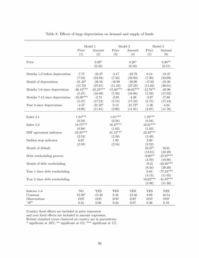
Table 8: Effects of large depreciation on demand and supply of funds

Model 1 Model 2 Model 3Price Amount Price Amount Price Amount(1) (2) (3) (4) (5) (6)

Price 0.29* 0.28* 0.30**(0.16) (0.16) (0.15)

Months 1-3 before depreciation -7.77 -23.27 -4.17 -23.79 0.14 -18.27(7.52) (23.94) (7.34) (23.93) (7.30) (23.69)

Month of depreciation -21.42* -28.58 -16.99 -28.90 -17.83 -21.93(11.72) (37.61) (11.43) (37.59) (11.62) (38.01)

Months 1-6 since depreciation -26.13*** -45.23*** -15.83*** -46.62*** -12.76** -20.98(5.47) (16.89) (5.56) (16.88) (5.59) (17.02)

Months 7-12 since depreciation -16.38*** -2.74 -3.95 -4.39 -2.97 17.88(5.47) (17.52) (5.74) (17.52) (5.72) (17.44)

Year 2 since depreciation -4.57 -21.52* 0.13 -21.72* -1.36 -4.84(3.90) (11.81) (3.90) (11.81) (3.87) (11.76)

Index 5.1 1.84*** 1.61*** 1.70***(0.59) (0.58) (0.58)

Index 5.2 18.75*** 16.27*** 16.61***(0.98) (1.02) (1.03)

IMF agreement indicator 22.45*** 21.12*** 22.33***(2.52) (2.50) (2.49)

Sudden stop indicator 0.67 1.93 2.00(2.59) (2.54) (2.52)

Month of default 23.37* 16.61(13.01) (42.49)

Debt rescheduling process -9.60** -47.87***(3.79) (10.98)

Month of debt rescheduling -9.21 -82.05***(9.34) (29.49)

Year 1 since debt rescheduling 6.04 -77.24***(4.15) (11.05)

Year 2 since debt rescheduling 18.62*** -41.97***(3.38) (11.38)

Indexes 1-4 NO YES YES YES YES YESConstant 12.29* -15.46 8.48 -13.40 8.89 16.54Observations 2197 2197 2197 2197 2197 2197“R2” 0.31 0.06 0.34 0.07 0.36 0.10

Country fixed effects are included in price regressionand year fixed effects are included in amount regression.Robust standard errors clustered on country are in parentheses.* significant at 10%; ** significant at 5%; *** significant at 1%.

30

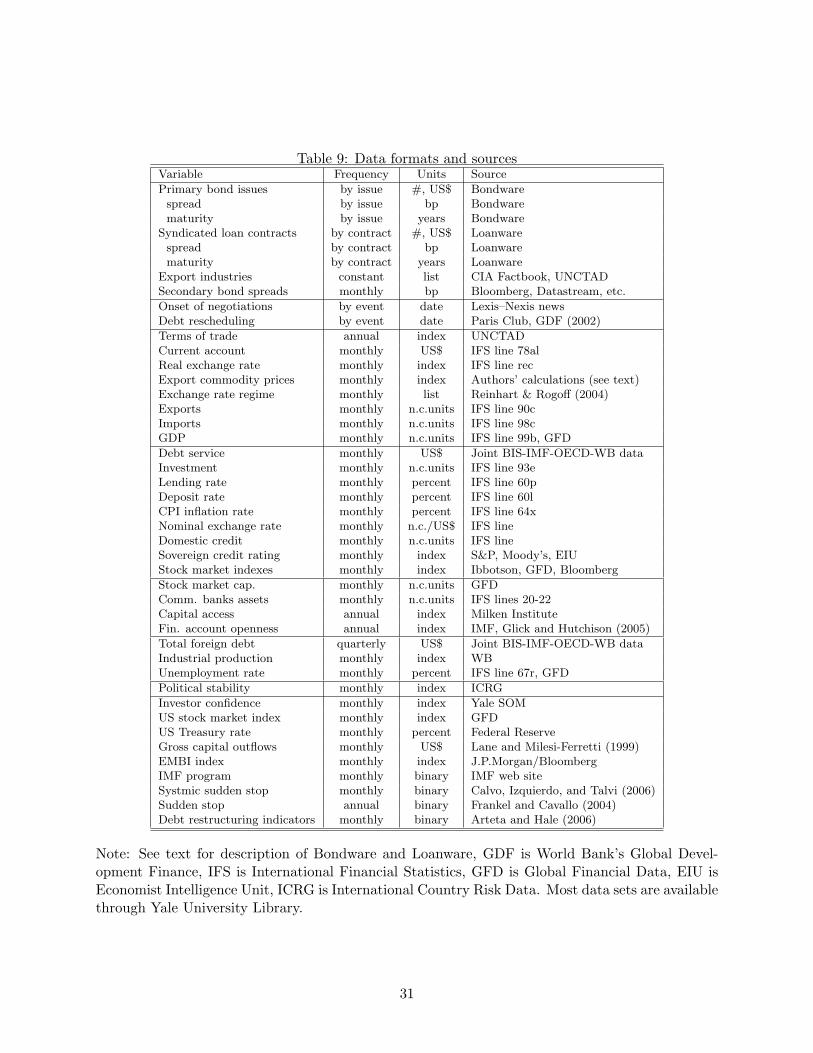
Table 9: Data formats and sourcesVariable Frequency Units Source

Primary bond issues by issue #, US$ Bondwarespread by issue bp Bondwarematurity by issue years Bondware

Syndicated loan contracts by contract #, US$ Loanwarespread by contract bp Loanwarematurity by contract years Loanware

Export industries constant list CIA Factbook, UNCTADSecondary bond spreads monthly bp Bloomberg, Datastream, etc.

Onset of negotiations by event date Lexis–Nexis newsDebt rescheduling by event date Paris Club, GDF (2002)

Terms of trade annual index UNCTADCurrent account monthly US$ IFS line 78alReal exchange rate monthly index IFS line recExport commodity prices monthly index Authors’ calculations (see text)Exchange rate regime monthly list Reinhart & Rogoff (2004)Exports monthly n.c.units IFS line 90cImports monthly n.c.units IFS line 98cGDP monthly n.c.units IFS line 99b, GFD

Debt service monthly US$ Joint BIS-IMF-OECD-WB dataInvestment monthly n.c.units IFS line 93eLending rate monthly percent IFS line 60pDeposit rate monthly percent IFS line 60lCPI inflation rate monthly percent IFS line 64xNominal exchange rate monthly n.c./US$ IFS lineDomestic credit monthly n.c.units IFS lineSovereign credit rating monthly index S&P, Moody’s, EIUStock market indexes monthly index Ibbotson, GFD, Bloomberg

Stock market cap. monthly n.c.units GFDComm. banks assets monthly n.c.units IFS lines 20-22Capital access annual index Milken InstituteFin. account openness annual index IMF, Glick and Hutchison (2005)

Total foreign debt quarterly US$ Joint BIS-IMF-OECD-WB dataIndustrial production monthly index WBUnemployment rate monthly percent IFS line 67r, GFD

Political stability monthly index ICRG

Investor confidence monthly index Yale SOMUS stock market index monthly index GFDUS Treasury rate monthly percent Federal ReserveGross capital outflows monthly US$ Lane and Milesi-Ferretti (1999)EMBI index monthly index J.P.Morgan/BloombergIMF program monthly binary IMF web siteSystmic sudden stop monthly binary Calvo, Izquierdo, and Talvi (2006)Sudden stop annual binary Frankel and Cavallo (2004)Debt restructuring indicators monthly binary Arteta and Hale (2006)

Note: See text for description of Bondware and Loanware, GDF is World Bank’s Global Devel-opment Finance, IFS is International Financial Statistics, GFD is Global Financial Data, EIU isEconomist Intelligence Unit, ICRG is International Country Risk Data. Most data sets are availablethrough Yale University Library.

31