current topics in cost allocation and custom api ... words: cost allocation, ibm cognos tm1, php,...
TRANSCRIPT

University of Economics in Prague
Faculty of Informatics and Statistics
Department of Information Technology
Study program: Applied Informatics
Specialization: Information Systems and Technology
Current topics in cost allocation
and custom API development
in IBM Cognos TM1
Diploma thesis
Student : Bc. Peter Fedoročko Supervizor : doc. Ing. Jan Pour, CSc.
Objector : Ing. Ondřej Bothe
2012

Enouncement
I honestly declare that I have prepared my bachelor thesis by myself and that I have adduced all
resources and literature I used.
Prague, 12.11.2012 ......................................................
Bc. Peter Fedoročko

Acknowledgement
I would like to thank my supervisor, doc. Ing. Jan Pour, CSc., for his continual support and advice
throughout this work and my colleagues from IBM for many helpful reflections.

Abstrakt
Diplomová práca sa orientuje na súčasné trendy prístupu k nákladovej alokácii v nástroji IBM Cognos
TM1. Koncept, ktorý bol po prvýkrát rozpracovaný v mojej bakalárskej práci, začal v poslednom čase
narážať na obmedzenia, spôsobené zvyšujúcimi sa nárokmi na analytické nástroje a informácie, ktoré
poskytujú. Cieľom práce je preto analyzovať príčiny vznikajúcich slabín, navrhnúť a implementovať
optimalizované riešenie spĺňajúce súčasné požiadavky. Vzhľadom na kvantitatívne zhodnotenie
dosiahnutých výsledkov je práca rozšírená o analýzu rámcov a štandardov určených na porovnávanie
OLAP nástrojov a ich syntézu do vlastného komplexného modelu. Model sa špecializuje na meranie
viacerých OLAP aplikácií cez 4 základné perspektívy obsahujúce výkon, vývoj, použiteľnosť a finančné
benefity. Dosiahnuté výsledky potvrdzujú, že inovovaný model je rýchlejší, bohatší na informácie,
jednoduchší na použitie a vhodný pre organizácie so štrukturovaným a algoritmickým prístupom k
nákladovej alokácií. Druhá časť práce sa zameriava na rozšírenie prezentačnej vrstvy aplikácie do
webového rozhrania a vývoj typizovaných vizualizácií pre najrozšírenejšie analytické úlohy. Vzhľadom
na absenciu pokročilého aplikačného rozhrania nástroja IBM Cognos TM1 je práca rozšírená o
teoretickú analýzu súčasných trendov pri vývoji API a následným návrhom konceptu, umožňujúcim
komunikáciu a predávanie dát medzi aplikáciou a TM1 serverov. V záverečnej časti práce je koncept
zhmotnený do univerzálnej knižnice vyvinutej v jazyku PHP a aplikovaný na aktualizovaný model
alokátora. Využitím knižnice sú následne vyvinuté dve vzorové koncepty rozhraní pre ovládanie a
prácu s modelom. Získané poznatky môžu slúžiť ako podklad pre vývoj ďalších komponentov
komunikujúcich s TM1 v najrozšírenejšej palete projektov alebo ako teoretický základ pri tvorbe API
vo všeobecnosti.
Kľúčové slová: cost allocation, IBM Cognos TM1, PHP, TM1 API, Raphael
Abstract
Thesis is devoted to current trends in approaching cost allocation developed in IBM Cognos TM1
software. Concept, which was originally elaborated in my bachelor thesis, has recently experienced
restrictions caused by increasing requirements on analytical tools and information they provide. Goal
of the thesis is therefore to analyse causalities of emerging weaknesses, design and develop
optimalized and reengineered solution answering current demands. Reqarding the quantitative
evaluation of attained results, the thesis is extended with analysis of frameworks and standards
dedicated to benchmarking of OLAP tools and their synthesis into own complex model. Proposed
model specializes on measuring multiple OLAP applications across four main perspectives including
performance, development, usability and financial benefits. Attained results prove, that
reengineered model is faster, data richer, easier to use and appropriate for any organization with
structured and algorithmic approach to cost allocation. Second half of the thesis focuses on
extending the presentation layer to web browser, designing and developing of custom visualizations
for most usual analytic tasks. Considering the absence of advanced application interface in IBM
Cognos TM1, the thesis also includes theoretical analysis of current trends in API development and
design of concept allowing communication and data transportation between applications and TM1
server. In the concluding section of the thesis, proposed concept is materialized into universal library
developed in PHP and applied to novel allocation model. Leveraging the library, two exemplary
interfaces for allocator operation and data consumption are implemented. Gained knowledge can
serve as basis for development of additional components communicationg with TM1 in variety of
projects or theoretical framework for API implementation in general.
Key words: cost allocation, IBM Cognos TM1, PHP, TM1 API, Raphael

Content
1. Introduction .................................................................................................................................................... 9
1.1. Reason and scope of the thesis.................................................................................................................. 9
1.2. Thesis Goals ............................................................................................................................................. 10
1.3. Thesis structure ........................................................................................................................................ 10
1.4. Applied methodologies ............................................................................................................................ 10
1.5. Thesis contributions ................................................................................................................................. 11
1.6. Assumptions and restrictions ................................................................................................................... 12
2. Characteristics of the current state .............................................................................................................. 13
2.1. Cost allocation implementations ............................................................................................................. 13
2.2. OLAP models benchmarking .................................................................................................................... 14
2.3. Software integration ................................................................................................................................ 15
2.4. Data visualization techniques .................................................................................................................. 15
3. Characteristics of current cost allocation principles .................................................................................... 17
3.1. Cost allocation theory and general principles .......................................................................................... 17
3.2. Cost allocation implementation environment ......................................................................................... 19
3.3. Standard Waterfall Cost Allocator ........................................................................................................... 20
3.4. Standard allocator issues ......................................................................................................................... 23
3.4.1. Speed of calculation ............................................................................................................................ 23
3.4.2. Volume of data .................................................................................................................................... 25
3.4.3. Tracing of cost flow ............................................................................................................................. 25
3.4.4. Interpretation of results ...................................................................................................................... 26
3.4.5. Complexity of rules and processes ...................................................................................................... 27
3.5. Analysis of existing issues and reengineering hypothesis ........................................................................ 27
3.6. OnDemand Allocator solution design ...................................................................................................... 32
3.6.1. Source Structure .................................................................................................................................. 32
3.6.2. Target structure ................................................................................................................................... 33
3.7. onDemand Allocator solution implementation ....................................................................................... 41
3.7.1. Source Structure .................................................................................................................................. 42
3.7.2. Trace Cube ........................................................................................................................................... 43
3.7.3. Advanced trace visualization ............................................................................................................... 44
3.7.4. Processes ............................................................................................................................................. 45
3.8. Standard vs. onDemand solution benchmarking ..................................................................................... 48
3.8.1. Benchmarking metrics definition ........................................................................................................ 48
3.8.2. Defined goals ....................................................................................................................................... 54

3.8.3. Benchmarking Results ......................................................................................................................... 54
4. Custom TM1 API and Advanced Visualization .............................................................................................. 61
4.1. Custom TM1 API....................................................................................................................................... 62
4.1.1. Request processing .............................................................................................................................. 63
4.1.2. Response composing ........................................................................................................................... 68
4.1.3. Request invocating .............................................................................................................................. 70
4.1.4. Response processing ........................................................................................................................... 71
4.2. onDemand allocator API .......................................................................................................................... 72
4.2.1. Selection object ................................................................................................................................... 73
4.2.2. Trace object ......................................................................................................................................... 73
4.3. onDemand allocator alternative visualizations ........................................................................................ 76
4.3.1. Comparison tree visualization ............................................................................................................. 81
4.3.2. Ad-hoc Drill visualization ..................................................................................................................... 84
5. Conclusion .................................................................................................................................................... 88
6. Terminology ................................................................................................................................................. 90
7. Resources ..................................................................................................................................................... 91
8. List of visualizations ...................................................................................................................................... 96
9. List of tables ................................................................................................................................................. 97
10. Appendix A ............................................................................................................................................... 98
10.1. Code Snippets ...................................................................................................................................... 98
10.1.1. Code Snippet A – Main Allocation ....................................................................................................... 98
10.1.2. Code Snippet B – Tracing Cube ............................................................................................................ 99
10.1.3. Code Snippet C – Advanced Tracing .................................................................................................. 100
10.1.4. Code Snippet D – Trace Delete Process ............................................................................................. 101
10.1.5. Code Snippet E – Start Drill Process .................................................................................................. 102
10.1.6. Code Snippet F – Allocation Process .................................................................................................. 102
10.1.7. Code Snippet G – Crawl Element Process .......................................................................................... 103
10.1.8. Code Snippet H – Crawl Value Process .............................................................................................. 105
11. Apendix B ............................................................................................................................................... 108
11.1. Benchmarking Results ....................................................................................................................... 108
11.1.1. Hardware Performance – CPU ........................................................................................................... 108
11.1.2. Algorithm Performance – Full Load ................................................................................................... 109
11.1.3. Algorithm Performance – Ad-hoc ...................................................................................................... 110
11.1.4. Model Complexity ............................................................................................................................. 111
12. Appendix C ............................................................................................................................................. 112
12.1. Code Snippets .................................................................................................................................... 112
12.1.1. Code Snippet I – executeProcess function / api.php ......................................................................... 112

12.1.2. Code Snippet J – driver.php class ...................................................................................................... 112
12.1.3. Code Snippet K – getData function / api.php .................................................................................... 114
12.1.4. Code Snippet L – AJAX GET method .................................................................................................. 114
12.1.5. Code Snippet M – AJAX POST method ............................................................................................... 114
12.1.6. Code Snippet N - Selection object ..................................................................................................... 115
12.1.7. Code Snippet O – Trace object .......................................................................................................... 116
13. Appendix D ............................................................................................................................................. 118
13.1. Code Snippets .................................................................................................................................... 118
13.1.1. Code Snippet P – Invoke allocation ................................................................................................... 118
13.1.2. Code Snippet Q –Comparison tree processing on received data ...................................................... 120
13.1.3. Code Snippet R – Invoke drill function .............................................................................................. 121
13.1.4. Code Snippet S – Change visibility function ....................................................................................... 121
13.1.5. Code snippet T – Hovering functions ................................................................................................. 122
13.1.6. Code snippet U – Recolor all levels functions .................................................................................... 123
13.1.7. Code snippet V – Bounce interferring nodes ..................................................................................... 123
13.1.8. Code snippet X – Drill-down ad-hoc processing of received data ..................................................... 124
13.1.9. Code snippet Y – Focus node function .............................................................................................. 125
13.1.10. Code snippet Z – Offset node function ............................................................................................... 126
9
1. Introduction
1.1. Reason and scope of the thesis
As the whole enterprise software industry continuously shifts toward new trends and technologies, it
simultaneously challenges existing solutions to conform to increasing requirements and novel
standards. What used to be fast, accurate and business needs sufficient two to three years ago is
now slow, vague and far behind current business demands. The same destiny has been reaching
standard cost allocation engine I introduced in my bachelor thesis. Despite its multiple
implementations in the fore-passed period, increasing number of voices from customers and
business partners with taunt tone objecting performance and usability of the solution has emerged.
Moreover, during the search for a proper cure, integration issues and API absence of software used
for allocator implementation arose, what significantly decreased recovery possibilities and allocator’s
future competitive edge. Because of the belief that the designed general API could solve not only
current visualization issues however can be ground-breaking for various implementations, serial of
articles probing the community interest has been published. Their readability and received feedback
confirmed that the topic is advisable to solve and can have a high added value.
Both mentioned reasons represented initial impulse of interest and led to the yearlong research and
experimentation. This research is documented in the thesis and addresses two main subjects. With
intention to put the allocation solution back to game, my work focuses on existing cost allocation
solution analysis and its reengineering with novel approach. The novel approach is however
presented with accent on solution independency and versatility and therefore suitable for
organizations with existing standard allocation concept as well as for units in early stage of
deployment. Moreover, the versatility of presented findings makes the solution applicable to wide
audience of public and private organizations meeting the condition of extensive but algorithmic
approach to allocation methodology. Secondly, the topic is extended with analysis of current
practices and possibilities in API development, design of general interface for employed IBM Cognos
TM1 software and application of these practices to reengineered allocation solution. The scope is
valuable not only for organizations aiming to leverage wider visualization capabilities of novel
allocator however for everyone with intention to integrate and invoke communication with TM1
from outside the native environment.

10
1.2. Thesis Goals
Presented scope has determined core goals of the thesis to be design of reengineered allocation
methodology and development of general custom TM1 application programming interface. In
order to fulfil these missions, set of partial goals need to be solved. The fractional objectives include:
Identification of key standard allocator weaknesses and their analysis
Validation of collected reengineering hypothesis and their implementation
Development of general and complex framework for benchmarking OLAP models
Analysis of current best practices in API development and its design for TM1
Analysis of alternative forms of allocation visualization and their implementation
1.3. Thesis structure
Thesis is divided into two core building blocks aligned with two main objectives. While the first part
focuses on design of reengineered allocation methodology, the second half of the thesis addresses
development of general custom TM1 application programming interface. Furthermore, the section of
allocation methodology reengineering is divided into three blocks targeting gradually its fractional
objectives. The analysis of standard allocator weaknesses is followed by validation of collected
reengineering hypothesis. Eventually, the development of general benchmarking framework is
discussed. The application programming interface part is separated into two sections discussing the
development of TM1 API and subsequently its application to reengineered allocator in order to build
alternative visualizations.
1.4. Applied methodologies
Various methodologies were applied in fractional blocks throughout the thesis with intention to fulfil
their goals. For the purpose of standard allocator weaknesses identification, numerous interviews
with customers and involved business partners have been conducted. Interviews focused on
collecting current objections which were subsequently quantitatively evaluated to determine their
effects and translated into initial hypothesis, anticipating the existence of improved solution.
Additionally, techniques used by strategic consulting firms were applied to examine and validate
11
reengineering premises. It required particular hypotheses to be subjected to data driven analyses
and empirical experiments in order to confirm their veracity. On the other hand, the development of
benchmarking framework was based on analyses of existing methodologies for evaluating both OLAP
and enterprise software in general. Whereas there does not exist complex framework for
benchmarking different models within single engine, the particular methodologies were reduced and
selected metrics composed into conforming structure. Similarly, the custom TM1 API design emerged
from analyses of current best practices and techniques used for interfaces development while
individual recommendations were subjected to numerous experiments testing the capabilities of
available software components and their functionality. Eventually, the various advanced visualization
have been developed and empirically tested on potential users to identify the most appropriate and
suitable forms.
1.5. Thesis contributions
Thesis provides valuable source of information for various groups of readers. Organizations
considering deployment of cost allocation solution or units searching improvements in their current
implementation can utilize and find the instigations for novel and alternative approach to allocation
with improved performance and usability results. In addition, different visualization forms and their
determination for specific purposes are suggested, which can be used to improve practicability and
readability of allocation tasks and results. On the other hand, TM1 and OLAP developers in general,
can find thesis useful for its complex benchmarking framework consolidating various standards and
allowing evaluation and comparison of different OLAP models and implementations. For developers
interested in communicating with TM1 from outside native environment, thesis provides theoretical
basis and practical guide for developing their own API. However, thanks to the universal approach to
proposed interface, majority of concepts can be also leveraged by general audience seeking options
for opening their solution to other systems. Except to major contributions, thesis as whole can serve
well as introduction to cost allocation problematic and review of options for its technical
implementation.

12
1.6. Assumptions and restrictions
Because of the theoretical introduction to cost allocation methodology in my previous thesis, current
work does not repeat in detail core concepts and focuses more on technical aspects and options of
allocation deployment. Furthermore, reengineering assumptions emerging from the standard
allocator analysis are restricted to single condition of the same data input as the original version.
Thesis also expects that reader is familiar with the OLAP technology and core concepts of IBM
Cognos TM1 software necessary for understanding the allocator’s implementation part. Similarly, the
knowledge of software integration and API principles is required. On the other hand, the elaborated
solutions were restricted to use of IBM Cognos TM1 and open source technologies. Additionally, the
hardware used for evaluating and comparing developed models allowed only smaller models to be
benchmarked.

13
2. Characteristics of the current state
2.1. Cost allocation implementations
Regarding the uniqueness of every institution and its business processes in current era, the
controlling and financial community is marked with the absence of a unified opinion about
methodology and even technology used when solving more demanding costing and budgeting tasks.
This perception can be confirmed by numerous publications suggesting various software approaches
especially to extremely peculiar cost allocation. Numerous authors (KELLER, 2005, p. 25; LEESE, 2009,
p. 56) and even institutions (U.S. DEPARTMENT OF EDUCATION, 2009, p. 17; VOLLMERHAUSE, 2009,
p. 15) propose solutions leveraging table calculator’s capabilities such as functions and Macros in
Microsoft Excel. In addition to custom developed applications, an array of software vendors offering
proprietary solutions based on relational databases have emerged (ACORN SYSTEMS, 2012;
CUBEBILLING, 2012; TAGETIK, 2012). Eventually cost allocation has become inseparable component
of many huge enterprise suits (SAGE PFW, 2009, ORACLE, 2009, p. 4; SALMON, 2011, p. 497).
However, there are many authors pointing to the disadvantages of spreadsheet technology with
major objections focusing on security weaknesses, integrity issues and lack of control (FEST, 2007, p.
1; BARNES, 2006, p. 1; NOORVEE, 2007, p. 69). Furthermore others (BOTHE, 2007, p. 8; MARTIN,
2008, p. 30) declare, that heterogeneousness and convertibility of organization’s environment and
conditions cause frequent adjustments to the allocation mechanism, which could be hard to follow
and simulate in generic software solutions (black-boxes). Therefore in my bachelor thesis
(FEDOROČKO, 2010a, p. 29) I elaborated a notion of implementing cost allocation in
multidimensional OLAP technology. The idea is supported by three crucial facts. OLAP
multidimensional cube space conforms well to cost allocation principle defined as matrix of objects
and their relations (POPESKO, 2009, p. 55; FIBÍROVÁ, 2007, p. 129). Secondly, the OLAP technologies
are in particular designed for business end-users and therefore allow agile adjustments to the
allocation model without professional intervention (BOTHE, 2007, p. 7; MUNDY, 2002, p. 22).
Eventually, the OLAP in-memory technologies achieve great performance results necessary for
complicated calculations over data with high granularity (ZANAJ, 2012, p. 5; MUNDAY, 2002, p. 22).
According Gartner’s 2011 Magic Quadrant for Corporate Performance Management Suits, IBM
Cognos TM1 was evaluated as one of the three leading OLAP solutions (GARTNER, 2010, p. 2). Based
on this strong position and my personal proficiency with the software, it was selected as
implementation environment for cost allocation solution.

14
Despite mentioned efforts have led to multiple implementations during last two years, some issues
and recommendations have occurred from early discussions with customers (BOTHE, 2010) and
involved business partners (BOTHE, 2011). Arguments further analyzed in this thesis have focused
mainly on performance improvements and user experience perspective. However as many sources
declare (GARTNER, 2011, p. 7; OKTAY, 2007, p. 227), these topics are caused by continuous increase
in requirements and apply to majority of Business Intelligence and enterprise software products in
general.
Discussed issues and new capabilities of chosen software allowed reengineering existed solution
from bachelor thesis and modifying it to meet the needs of accumulated requirements. This work
focuses on the analysis of collected problems as well as design and proposes implementation steps
for new solution.
2.2. OLAP models benchmarking
Currently, there does not exist complex framework for benchmarking two different implementations
of OLAP models. In 1998 OLAP Council contributed to the development of an analytical processing
benchmark called APB-1, which defines set of metrics used for comparing various OLAP software
(OLAP COUNCIL, 1998, p. 3). Despite framework focuses on software benchmarking, particular
metrics can be also used to distinguish performance of different models within single engine. The
core performance metrics of APB-1 are time to perform batch operations and number of queries
executed. Another source for benchmarking provides international norm ISO/IEC 25000:2005 which
within its Software Product Quality Requrements and Evaluation (SQuaRE) framework defines six
metrics for evaluating software quality (ISO/IEC 25000, 2005, p. 10). These metrics go beyond
traditional performance issues and embrace factors such as usability, maintainability and
functionality, what makes them ideal for applying to concurrent OLAP models. Whereas the usability
and user experience have been strong arguments against traditional model, it is necessary to place
even bigger importance on its benchmarking. This topic is fortunately heavily discussed in enterprise
as well as end-user software environment. Comprehensive overview of methods for evaluating
software usability provides Fitzpatrick (1998, p. 5). In his work three different frameworks by
acknowledged authors are introduced, researched and substantiated into composite list including
factors such as observation, questionnaire, interview or empirical methods. Similar overview
encompassing even broader palette of frameworks is introduced by Seffan. (2006, p. 161) Here
15
different standards or models within the Human-Computer Interaction (HCI) and the Software
Engineering (SE) communities have been researched.
2.3. Software integration
Software integration and interoperability via Application Programming Interfaces (API) as well as the
emergence of web services computing model for connecting disparate systems is a hot topic and
inseparable component of every software package these days (SPOFFORD, 2006, p. 46). Despite that,
IBM Cognos TM1 still does not provide standard interface for accessing objects from outside the
native environment. Although simple TM1 API does exist, it is restricted to basic components
invokation and does not provide capabilities for developing complex applications on top of existing
models (IBM, 2011, p. 47). Several third party vendors (CARPEDATUM, 2012) and developers
(GYANWALI, 2007) have expressed efforts to offer customized solutions, however these are either
dependent on provider’s services or do not allow easily executable input and output commands. The
absence can be solved, as suggested by numerous web communities, by implementing own
interface. These communities propose well documented general suggestions (ALARCON, 2011) and
best practices (MULLOY, 2012) explaining how to develop proprietary REST API by using different
server side scripting languages. The result is a set of unique URLs enabling access to required data.
This URL when requested with set of mandatory parameters returns XML or JSON formatted
response. However, in order to invoke internal TM1 data processing via REST request, the standalone
executable utility which is part of TM1 has to be leveraged. This is well documented in various
sources (IBM, 2011b; FEDOROČKO 2012a). The guidelines for turning TM1 data into XML format are
included in standard documentation (SLEIGH, 2010, p.4), while JSON formatted output is result of
various experimentations firstly described in my blog post (FEDOROČKO, 2012b).
2.4. Data visualization techniques
Rich source for client-centric OLAP visualization techniques can be found in Hsiao research (2011, p.
75). Research proposes architectural foundations for building interactive visualizations in web
browser using native scripting languages. Particular visualization methods are heavily discussed in
numerous articles and academic researches (MANSMANN, 2007, p. 2; SCHUTZ, 2011, p. 8). Bordley
in his work (2002, p. 140) introduced concept of leveraging tree and donut scheme as supplements

16
for table space information presentation. Tree layout is ideal for visualizing problem structure,
strength of relations and values of nodes. Mansmann (2007, p. 3) also suggests leveraging color
pallet to distinguish quantitative information related to nodes instead of their radiuses. Addition they
declare tree structure to be especially suitable for non-technical audience. Despite Bordley proposed
using Microsoft Excel for visualizations (2002, p. 139), several authors suggest focusing on web-based
interface when considering application requirements (HSIAO, 2011, p. 77; MEKTEROVIĆ, 2005, p. 2).
This has been supported by various sources declaring following advantages. The web front-end
languages and frameworks provide agile approaches to requesting and processing data via REST APIs
(LENGSTORF, 2010, p. 78). Additionally, popularity of Web 2.0 applications initialized development of
technologies and frameworks for rich and dynamic data presentation. Several authors and
developers have introduced libraries (BARANOVSKIY, 2012) and guidelines (SHARP, 2010, p. 279) for
creating and manipulating advanced graphic objects in web browser.

17
3. Characteristics of current cost allocation principles
3.1. Cost allocation theory and general principles
Popesko (2009, p. 55) in his publication defines allocation as: “Assignation of cost, margin, revenue,
price or any other value to product, service, activity, operation or any other natural unit. “ Similarly,
Fibírová (2007, p. 129) equals it to: “Recalculation of quantitative value to naturally expressed unit of
performance, product, service, work or operation affiliated with creation of this performance.” From
international sources, Hansen (2009, p. 219) refers to allocation as: “Division of pool of costs and
their assignment to various subunits”. Drury (2008, p. 48) on the other hand liken it to: “The process
of assigning cost when a direct measure does not exist for the quantity of resources consumed by a
particular cost object.”
However, cost allocation topic is not discussed only at academic soil but has many applications in
private as well as public sector. Despite, every organization tailors definition to its particular needs,
mutual features are drew and can be identified across all of them. Taking in consideration these
features and predominantly practical and implementation notion of the thesis over pure theoretical
disputation on the topic of corporate finance, I will further restrict cost allocation definition to:
“Recalculation of quantity from source unit to target unit based on their quantitative relation”. Even
though incomprehension-free construction at the first sight, it is necessary to explain some terms,
provide examples used for actual implementation and offer alternatives which could be integrated
into the mechanism without any impacts on prime behaviour. Terms are concluded in the following
table (Table 1).
Table 1 Core terms definition (Source: author)
Term Definition Used Value Alternative Value
Quantity Subject of allocation which will be transferred among
units based on their relations.
Cost Price, Margin, Revenue, Profit,
Material, Time
Unit Part of an organization which has assigned quantitative
metric and clear relation to other units.
Cost Center Employee, Product, Customer,
Partner, Supplier
Relation Link which is relevant to this relation and has
quantitative representation. Synonyms are key, driver.
Drivers Alternative drivers

18
While terms quantity and unit are strictly defined, relation is not restricted to obvious link, however
has deeper meaning in its quantitative valuation. The quantity usually referred as driver or key
includes several components. Except most obvious one, assigning part of source quantity to be
allocated to target object, final driver has to consider also internal rules determined by hierarchical
structure of units. These rules govern correct advancement in allocation execution and prevent not
authorized relations to be alleged. Based on the liberty of relations, three main types of cost
allocation can be identified (FEDOROČKO, 2010a, p. 27). Further disputation about the concept can
be found in my previous thesis or numerous books (HANSEN, 2009, p. 223; DRURY, 2008, p. 58) and
articles (LEESE, 2009, p. 55; BOTHE, 2009), where also deeper alignment with managerial accounting
practices is offered. Three types of allocation include:
Simple – In simple allocation units can strictly feature as provides (sources) or receivers (targets) of
quantity. There are no hidden rules and restrictions within the keys. Every relation is unidirectional
and noncyclical. This enables cost allocation to be executed in single step. While it is easy to
implement, the biggest disadvantage lays in poor alignment with complicated internal relations and
rules for governing the allocation (FEDOROČKO, 2010b, p. 4).
Waterfall – In different sources can be found also under terms cascade (Bothe, 2009) or Step-down
(LEESE, 2009, p. 55). In waterfall allocation, units can feature as both providers and simultaneously
receivers of quantity, while the condition of consecutiveness among units or unit groups has to be
maintained. This creates cascade of steps which has to be executed in order to gain final results. The
unidirectional fashion of relations however guarantee that entire value from provides will be
transferred to designed targets within single cycle. Feedbacks praise this method for better
conjunction with organizational environment and managerial accounting practices. On the other
hand, fully developed concept can reached significantly higher complexity that simple type
(FEDOROČKO, 2010b, p. 5).
Reciprocal – Is considered to be the most precise and advanced concept at all. Reciprocal allocation
attempts to simulate interval relations in the most scientific and exact way. It resembles waterfall
allocation while omits condition of consecutiveness. This creates bidirectional relations which have
to be executed in loops. Despite accurate results, reciprocal allocation is under critique for numerous
reasons. Firstly, opponents target to its implementation severity and requirements for looping
capabilities. Additionally, some raise objections that its alignment with internal relations goes at the
expenses of readability and easy orientation. Eventually, bidirectional relations bring possibility of
circular references what requires its proper handling and maintenance.
19
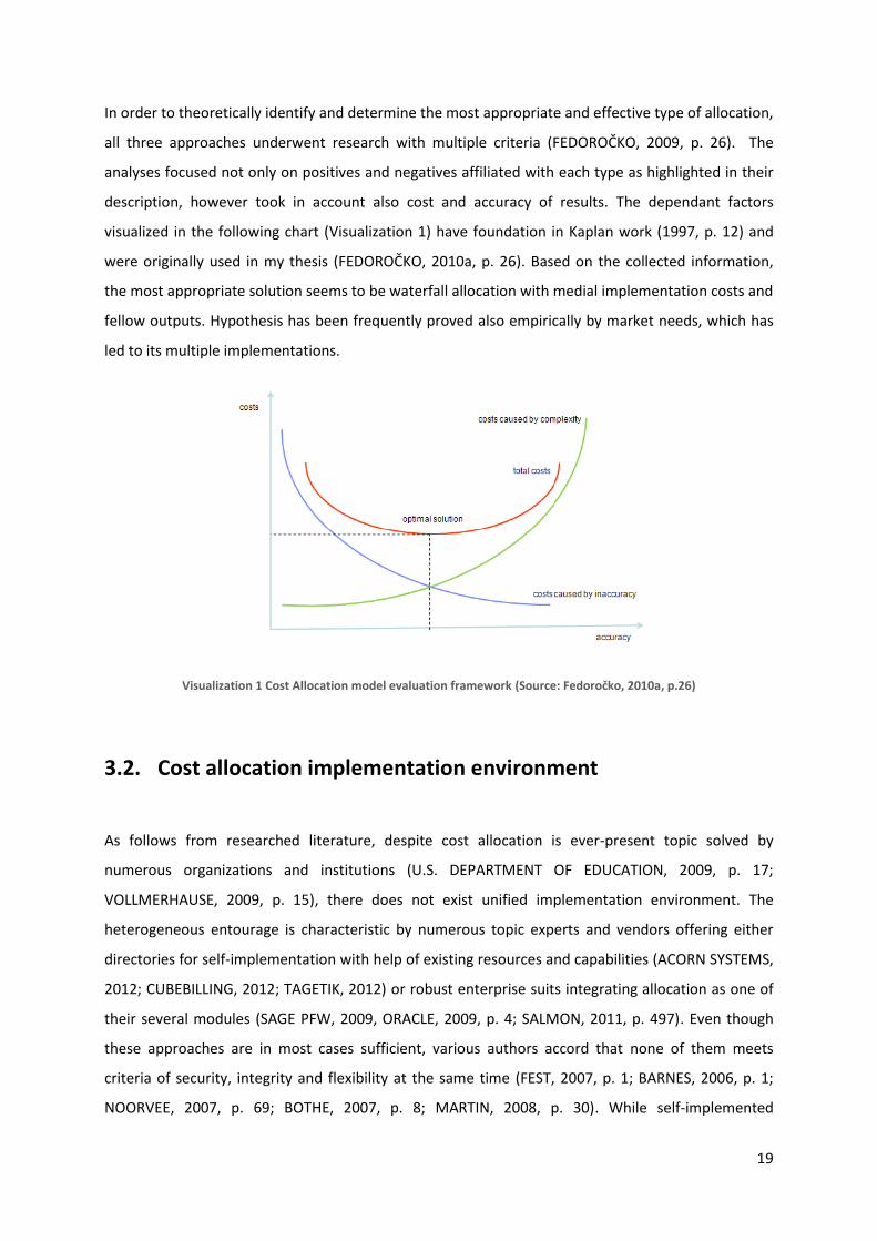
In order to theoretically identify and determine the most appropriate and effective type of allocation,
all three approaches underwent research with multiple criteria (FEDOROČKO, 2009, p. 26). The
analyses focused not only on positives and negatives affiliated with each type as highlighted in their
description, however took in account also cost and accuracy of results. The dependant factors
visualized in the following chart (Visualization 1) have foundation in Kaplan work (1997, p. 12) and
were originally used in my thesis (FEDOROČKO, 2010a, p. 26). Based on the collected information,
the most appropriate solution seems to be waterfall allocation with medial implementation costs and
fellow outputs. Hypothesis has been frequently proved also empirically by market needs, which has
led to its multiple implementations.
Visualization 1 Cost Allocation model evaluation framework (Source: Fedoročko, 2010a, p.26)
3.2. Cost allocation implementation environment
As follows from researched literature, despite cost allocation is ever-present topic solved by
numerous organizations and institutions (U.S. DEPARTMENT OF EDUCATION, 2009, p. 17;
VOLLMERHAUSE, 2009, p. 15), there does not exist unified implementation environment. The
heterogeneous entourage is characteristic by numerous topic experts and vendors offering either
directories for self-implementation with help of existing resources and capabilities (ACORN SYSTEMS,
2012; CUBEBILLING, 2012; TAGETIK, 2012) or robust enterprise suits integrating allocation as one of
their several modules (SAGE PFW, 2009, ORACLE, 2009, p. 4; SALMON, 2011, p. 497). Even though
these approaches are in most cases sufficient, various authors accord that none of them meets
criteria of security, integrity and flexibility at the same time (FEST, 2007, p. 1; BARNES, 2006, p. 1;
NOORVEE, 2007, p. 69; BOTHE, 2007, p. 8; MARTIN, 2008, p. 30). While self-implemented

20
applications by help of table calculators are unfitting for solutions leveraging and orchestrating
sensitive data from diverse sources, allocators in form of software modules are hard to flexibly and
independently curve according continuously altering conditions in current turbulent environment.
Based on the strong knowledge of cost allocation condensed in the previous paragraph and
capabilities of online analytical processing technology, the notion of its implementation in selected
OLAP software has been elaborated in my thesis (FEDOROČKO, 2010, p. 29), what I strongly believed
would eliminate obstacles affiliated with approaches currently used. In order to understand possible
impacts OLAP technology can have on highlighted arguments, it is necessary to firstly analyse its
characteristics. Online analytical processing has been firstly introduced by Edgar Codd in 1993 as a
supplement to relational data storages with huge emphasis on analytical tasks, performance
improvements, efficiency and user-friendly queries (GOIL, 1997, p. 53). Codd also listed 12 basic
characteristics of OLAP technologies. Factors relevant for cost allocation include: multidimensionality,
accessibility, stable access and performance, client-server architecture, operation on dimension or
intuitive manipulation of data. Summary of all rules provides i.e. Achor (200, p. 64) in his article on
OLAP tools. Taking in consideration these characteristics, it is obvious that multidimensional
specification conforms well with provided definition of cost allocation as matrix of relations.
Secondly, the client-server architecture removes obstacles affiliated with data integrity and security
over larger implementations while maintains required performance. Eventually the basic operations
on dimensions as well as intuitive manipulation of data and user friendly queries position OLAP
above general allocation modules in terms of flexibility and independent adjustments.
3.3. Standard Waterfall Cost Allocator
Based on the collected knowledge and identified proper technology, basics for cost allocation
deployment in OLAP environment has been firstly introduced in my thesis (FEDOROČKO, 2010, p. 29).
Despite thesis primarily focused on examination of reciprocal capabilities with available set of
functionality, it also encompasses intimate explanation of its core behaviour generic for all forms. For
the better understanding of issues affiliated with current standard implementation of waterfall
allocation and subsequent reengineering options, several necessary concepts need to be illustrated
prior to its analysis.
Taking in consideration allocation principle as map of relations it can leverage matrices within OLAP
multidimensional environment. However, in order to conform with internal rules and guidelines for
21
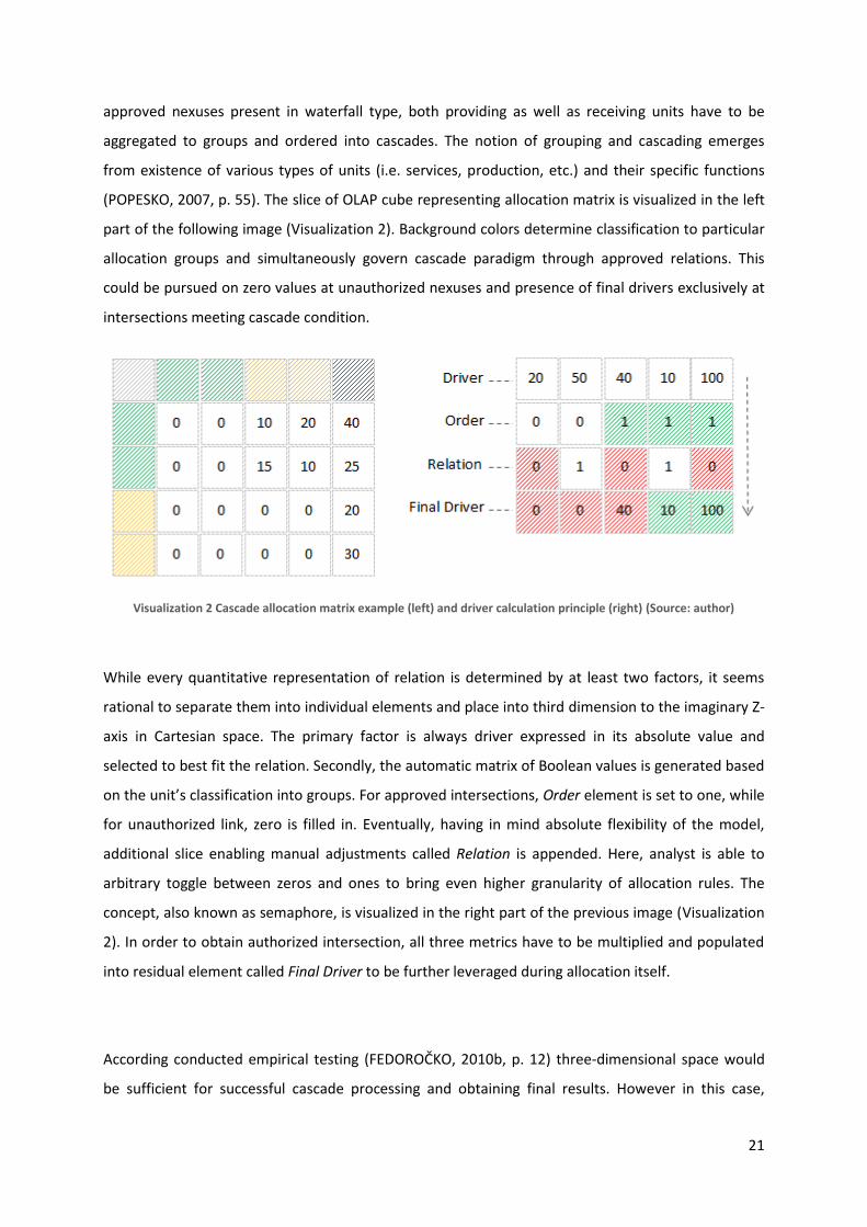
approved nexuses present in waterfall type, both providing as well as receiving units have to be
aggregated to groups and ordered into cascades. The notion of grouping and cascading emerges
from existence of various types of units (i.e. services, production, etc.) and their specific functions
(POPESKO, 2007, p. 55). The slice of OLAP cube representing allocation matrix is visualized in the left
part of the following image (Visualization 2). Background colors determine classification to particular
allocation groups and simultaneously govern cascade paradigm through approved relations. This
could be pursued on zero values at unauthorized nexuses and presence of final drivers exclusively at
intersections meeting cascade condition.
Visualization 2 Cascade allocation matrix example (left) and driver calculation principle (right) (Source: author)
While every quantitative representation of relation is determined by at least two factors, it seems
rational to separate them into individual elements and place into third dimension to the imaginary Z-
axis in Cartesian space. The primary factor is always driver expressed in its absolute value and
selected to best fit the relation. Secondly, the automatic matrix of Boolean values is generated based
on the unit’s classification into groups. For approved intersections, Order element is set to one, while
for unauthorized link, zero is filled in. Eventually, having in mind absolute flexibility of the model,
additional slice enabling manual adjustments called Relation is appended. Here, analyst is able to
arbitrary toggle between zeros and ones to bring even higher granularity of allocation rules. The
concept, also known as semaphore, is visualized in the right part of the previous image (Visualization
2). In order to obtain authorized intersection, all three metrics have to be multiplied and populated
into residual element called Final Driver to be further leveraged during allocation itself.
According conducted empirical testing (FEDOROČKO, 2010b, p. 12) three-dimensional space would
be sufficient for successful cascade processing and obtaining final results. However in this case,
22
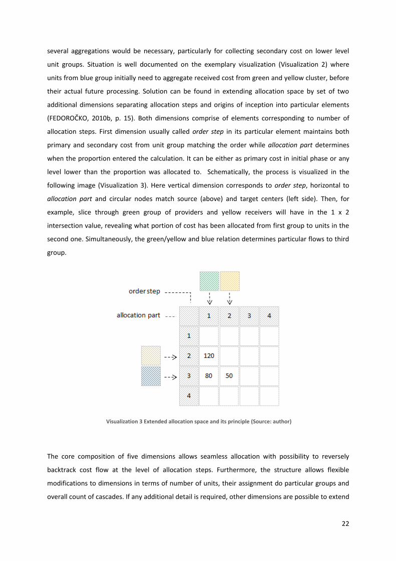
several aggregations would be necessary, particularly for collecting secondary cost on lower level
unit groups. Situation is well documented on the exemplary visualization (Visualization 2) where
units from blue group initially need to aggregate received cost from green and yellow cluster, before
their actual future processing. Solution can be found in extending allocation space by set of two
additional dimensions separating allocation steps and origins of inception into particular elements
(FEDOROČKO, 2010b, p. 15). Both dimensions comprise of elements corresponding to number of
allocation steps. First dimension usually called order step in its particular element maintains both
primary and secondary cost from unit group matching the order while allocation part determines
when the proportion entered the calculation. It can be either as primary cost in initial phase or any
level lower than the proportion was allocated to. Schematically, the process is visualized in the
following image (Visualization 3). Here vertical dimension corresponds to order step, horizontal to
allocation part and circular nodes match source (above) and target centers (left side). Then, for
example, slice through green group of providers and yellow receivers will have in the 1 x 2
intersection value, revealing what portion of cost has been allocated from first group to units in the
second one. Simultaneously, the green/yellow and blue relation determines particular flows to third
group.
Visualization 3 Extended allocation space and its principle (Source: author)
The core composition of five dimensions allows seamless allocation with possibility to reversely
backtrack cost flow at the level of allocation steps. Furthermore, the structure allows flexible
modifications to dimensions in terms of number of units, their assignment do particular groups and
overall count of cascades. If any additional detail is required, other dimensions are possible to extend
23
the model without impact on allocation logic. Based on the core, the implementation is also open to
further enhancement in terms of modules which are able to be plugged in via internal processes and
can server some specific logic. The standard examples are maintenance cubes handling driver,
relation and order mapping (FEDOROČKO, 2010b, p. 7) or cubes for extended tracing capabilities.
Whereas this concept has established and proved its viability many times during last two years, it will
be further in the text referred as standard allocator. Despite its popularity, several issues have been
consecutively identified. Following paragraphs aim to address these issues, analyse their effects and
propose alternative solutions.
3.4. Standard allocator issues
Since inception of standard allocator and during its implementations, some major and minor issues
have emerged from early discussions with customers (BOTHE, 2010) and business partners (BOTHE,
2011). These issues have not anyhow mitigated its value or restricted specified functionality and
flexibility, but rather have been results of natural advancements and increased standards for analytic
tools (GARTNER, 2011, p. 7). Main objections collected so far read:
Speed of calculation
Volume of data
Tracing of cost flow
Interpretation of results
Complexity of rules and processes
The roots, effects and possible solutions to five arguments are presented in the following sections.
3.4.1. Speed of calculation Standard cost allocation operates in the bulk mode when all possible combinations of data
representing cost flows are pre-calculated before user is able to observe final results. This requires
enormous amount of calculations to be executed, which can be expressed by following formula.
Calculation in case of allocation requires atomic operation of multiplication cost on source center by
driver assigned to the relation with target one. Formula assumes that number of cost centers in each
step is equal and all drivers are nonzero, so the maximum possible number of calculations will be
executed.

24
∑
[ (
)]
Table 2 Approximate number of calculations equation‘s variable definition (Source: author)
Variable Explanation
s Current allocation step
S Total number of allocation steps
C Number of cost centers
With respect to step of allocation (s), first multiplicator in equation represents number of source
centers, second number of receivers and third multiplicator number of steps of origin. Eventually, the
aggregation through all steps gives final count of operations needed to be executed. Formula can be
adjusted into the final equation with following form.
Table 3 Example of total calculations for various combinations of C and S (Source: author)
C S Ns
10 5 80
100 5 8 000
1000 5 800 000
100 10 16 500
1000 10 1 650 000
As could be seen in the previous table (Table no. 3), even small amount of input data results into
voluminous number of combinations leading to stream of time consuming operations and
consequent slower response durations. However, more important are particular increases of Ns for
relatively small enlargements of processed units. It is also necessary to highlight that production
solution of standard allocator would in addition to main matrix also allocate through other
dimensions, which can increase final count of calculations even more. This could lead in specific cases
to cubes with billions of calculations and significantly handicapped velocities.

25
3.4.2. Volume of data Volume of executed operations is also tightly linked to volume of generated data. While every value
obtained has to be stored in allocation structure and available for further processing in form of driver
or secondary cost as well as for eventual analysis, it places huge memory requirements on
infrastructure operating allocation engine. Based on the own empirical measurement, single
occupied cell demands 14B (bytes) of dedicated memory. The exemplary allocation structure with
one billion of records therefore would ask for approximately 13 GB of space.
3.4.3. Tracing of cost flow In allocation approach, cost flow is defined as string of cost centers representing in sequence how did
final quantity move among units and where did it stay before reaching target center. In case of ten
cascades, cost flows can be expressed as proposed in following table.
Table 4 Exemplary cost flows (Source: author)
Step 1 2 3 4 5 6 7 8 9 10
Cost flow 1 CC1 CC3 CC5 CC7 CC9 CC11 CC13 CC15 CC17 CC20
Cost flow 2 CC1 CC3 CC5 CC15 CC15 CC15 CC15 CC15 CC20 CC20
Cost flow 3 CC8 CC10 CC12 CC14 CC16 CC18 CC20
From the previous example, it is obvious that number of units in the string can be equal or lower
than number of cascades. It depends exclusively on fact, where did quantity enter allocation process.
In case of primary cost originating at cost center from subsequent step as one in the example of cost
flow 3, the string will be shortened to map of transfers from remaining cascades. Generally, two
conditions apply to cost flow formulation. Firstly, position of cost center within string has to
correspond to its actual placement within allocation order. In addition, quantity does not have to be
transferred in every step as visualized in the example of cost flow 2. In some cases, proportions are
allocated directly to units from distant cascades and wait there until allocation loop iterates to its
position. Taking in consideration this option, cost flow has to appropriately reflect this matter of fact
by extending the intermediate positions with quantity’s actual occurrence. In the second example,
cost center 5 prematurely allocated proportion to unit from eighth step. Therefore, all positions
between mentioned two cascades are filled with name of unit keeping the value until its further
processing.
Despite standard allocator includes two dimensions for tracking allocation steps as introduced at
page 22, the cost flow cannot by captured on the presented detail because of the aggregations of
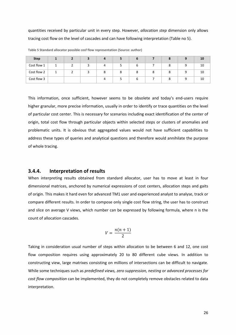
26
quantities received by particular unit in every step. However, allocation step dimension only allows
tracing cost flow on the level of cascades and can have following interpretation (Table no 5).
Table 5 Standard allocator possible cosf flow representation (Source: author)
Step 1 2 3 4 5 6 7 8 9 10
Cost flow 1 1 2 3 4 5 6 7 8 9 10
Cost flow 2 1 2 3 8 8 8 8 8 9 10
Cost flow 3 4 5 6 7 8 9 10
This information, once sufficient, however seems to be obsolete and today’s end-users require
higher granular, more precise information, usually in order to identify or trace quantities on the level
of particular cost center. This is necessary for scenarios including exact identification of the center of
origin, total cost flow through particular objects within selected steps or clusters of anomalies and
problematic units. It is obvious that aggregated values would not have sufficient capabilities to
address these types of queries and analytical questions and therefore would annihilate the purpose
of whole tracing.
3.4.4. Interpretation of results When interpreting results obtained from standard allocator, user has to move at least in four
dimensional matrices, anchored by numerical expressions of cost centers, allocation steps and gaits
of origin. This makes it hard even for advanced TM1 user and experienced analyst to analyse, track or
compare different results. In order to compose only single cost flow string, the user has to construct
and slice on average V views, which number can be expressed by following formula, where n is the
count of allocation cascades.
Taking in consideration usual number of steps within allocation to be between 6 and 12, one cost
flow composition requires using approximately 20 to 80 different cube views. In addition to
constructing view, large matrixes consisting on millions of intersections can be difficult to navigate.
While some techniques such as predefined views, zero suppression, nesting or advanced processes for
cost flow composition can be implemented, they do not completely remove obstacles related to data
interpretation.

27
3.4.5. Complexity of rules and processes Considering flexibility in number of allocation steps, standard allocator has to operate within one
modular data space in loops, where each loop represents recalculation of all source centers from
specific step identified by loop iterator. This approach however could be very prone to circular
references and data loses. In order to mitigate possible risks, allocation cycle has to be orchestrated
by set of rules, restrictions, complementary processes and subsidiary data spaces (FEDOROČKO,
2010b, p. 7). Logic behind the standard allocator therefore could not be so obvious and could
overwhelm conceptual understanding of common business user. Maintenance and business specific
requests such as additional rules, restrictions or processes within the loop can occur as impossible to
successfully implement by user’s own resources. Transparency and complexity of the solution
therefore goes at the expenses of user’s perception of control and ownership of the solution. This,
althought seen as soft metric, could be the most crucial for success of the implementation and
effectual adoption of the solution.
Current chapter introduced concept of standard allocator and analyzed the most important issues
affiliated with its design and operation. With intention to mitigate these weaknesses and propose
imporoved solution, next chapter will closely assess and evaluate hypotheses affiliated with presented
issues in order to validate the possibility of novel reengineered approach to cost allocation existence.
3.5. Analysis of existing issues and reengineering hypothesis
Previously discussed issues will serve as basis for reengineering reflection. The approach I selected to
mitigate or absolutely obliterate particular weaknesses emerges from practices used by top strategic
consulting firms firstly revealed by Rasiel (1999, p. 15). The framework consists of proper hypothesis
construction, continuous and data-rich set of analyses aiming to acknowledge and verify the
premises and final synthesis of collected information into final recommendation. Despite presented
problems are not even remotely close to complexity and extensiveness of actual issues frameworks
were developed to, it is good practice to apply them with purpose of maintaining focus on key pains,
easing the hypothesis verification and shifting to final synthesis substantiated into reengineered
solution. Whereas four issues have been proposed, I will address them with equal number of
separate premises. Hypothesis to counter the standard allocation approach are:
1. It is possible to provide on demand only results which are important for the user.
2. Visual representation of results can be more user-friendly with available resources.

28
3. It is possible to provide more detail data about cost flow while simultaneously decrease data
volumes and complexity of the solution.
4. Calculation engine can be less error prone and complex while transparency of code will be
maintained.
It is obvious that if all premises are positively answered, it is possible to develop solution which debugs
all existing issues and meets current standards and requirements demanded by standard allocator
users. The following paragraphs will focus on hypothesis analyses and verification. Eventually synthesis
of all finding will be executed and decision about existence of proper solution will be made.
1. It is possible to provide on demand only results which are important for the user.
The most significant issues such as speed of calculation, volume and complicated interpretation of
results are tightly bounded to massive and brute processing of every possible calculation. However in
practice, only few of them are subjects of user’s interest and further examination. If allocator is able
to focus its computation power to only these few flows, speed and volume would be decreased while
lucidity of results would improve. But could be all flows defined up front? In some cases, desired
relations are well defined but sometimes, analyst can decide which flows to follow only after she
observes final results or anomalies.
The current logic requires engaging all source centers to allocate and aggregate their particular cost
flows to single target value. The concept is visualized in the left part of the following image
(Visualization 4). However, if analyst is interested only in small number of cost flows (i.e. yellow one)
or finds the result corrupted and decides to subsequently look for anomalies, any other irrelevant
data and cost flows have consumed the computation power and memory unnecessarily.
Visualization 4 Reversed concept of the standard allocator (Source: author)

29
The solution can be found in reversing the whole concept as presented in the right part of the image
(Visualization 4). Here, the whole up front calculation is restricted to single final value without any
redundant cost flow processing or storing. Even after that, analyst is able to manually hand pick
desired flow, what leads to actual calculation (green one). The calculations are separated into smaller
execution steps, when definition of further proceeding has to be repeated at every level. It is obvious
that such transformation would lead to significant reductions to inevitable minimum and
simultaneously confirms the hypothesis of on demand processing. Maximal number of operations
within one level is possible to express by following formula.
Table 6 Maximal number of operations in onDemand allocator equation's variable definition (Source: author)
Variable Explanation
si Current allocation step
S Total number of allocation steps
C Number of cost centers
Having both formulas, numerical comparison of required calculations, hence, consumed data can be
conducted. Results for various dimension sizes are included in the following table (Table no. 6).
Table 7 Comparion of operations and volume for standard and reversed allocator (Source: author)
C S Ns NR
10 5 80 20
100 5 8 000 200
1000 5 800 000 2000
100 10 16 500 450
1000 10 1 650 000 4500
2. Visual representation of results can be more user-friendly with available resources.
Whereas the cost flow is composed of nodes (cost centers) and links (drivers) between these nodes,
the most nature visualization as proposed by numerous researches (BROADLEY, 2002, p. 140;
MANSMANN, 2007, p. 3) seems to be the tree structure, where the root is represented by target
center and its immediate descendants are cost centers allocating based on the relation. The reversed
allocator greatly resembles described structure, and therefore its usage would also support

30
verification of the second hypothesis. Moving and orientation on visually clear flat space of tree chart
is easier to understand than slicing across four dimensional matrix anchored by numerical
expressions of steps. In tree representation, step (level) of every center, its origin as well as provider-
receiver (child-parent) relation is clearly defined. Question remains, how can be tree chart graphically
visualized in flat table space such as view (cube slice) in IBM Cognos TM1. This can solve hierarchical
structure of dimensions in TM1. While vertical dimension would represent parent-child relation,
horizontal differentiation in each row would highlight allocation step (level). Further in the thesis, I
will further elaborate topic of advanced visualization and propose methods, how to transfer
complete presentation logic out of table-space to form tree and various other structures even more
precisely.
3. It is possible to provide more detail data about cost flow while simultaneously decrease data
volumes and complexity of the solution.
Thanks to significant reduction in number of required operations during identification of every cost
flow and removal of numerous aggregations on every cascade, it is obvious that reversal approach
can also be applied in case of more detail cost flow requirements. Heretofore speed and volume
savings can be instead of unnecessary operations used to more precise calculation of cost flow not
only at allocation step detail, but also at granularity of each transaction among particular centers.
The separation of cost flow definition to singular steps decremented number of possible transaction
within one procedure to Dd, what is value expressed by formula at page 29. Such value includes only
tenths or hundreds of necessary operations and makes it therefore viable to identify all transactions
within accepted response period. The hypothesis of more detailed data was also confirmed by
reversal allocation approach.
4. Calculation engine can be less error prone and complex while transparency of code will be
maintained.
As emerges from the analysis of first hypothesis, only data required to start reversed allocation are
final values on target centers. Obviously it still requires to somehow pre-allocate cost to the lowest
possible level, however focus purely on small set of eventual results as well as unnecessary to record
every available flow in this phase makes it possible to omit allocation step dimension tracing cost
origin. The exclusion suggests that number of required operations, before reversal allocation can be
applied, decrements to value expressed by the following formula. Variables are defined in Table 2 on
page 24.
[
]

31
Taking in consideration significant reduction in comparison to standard allocation severity, the
possibility to replace complex allocation regulas and procedures with expeditious recalculation
based-on set of rules simulating cascade iteration seems to be sufficient. In addition to this
replacement, the separation of allocation process into repeatable procedures subsequently
calculating desired values can also make the code more reusable and less complex. The reusability of
developed code however also influences its transparency and ease of use when future extensions are
about to be implemented. Taking in consideration all possible improvements and advantages, the
last hypothesis can also be considered as verified.
Conducted analyses proved and agreed that there does exist possible solution to all presented
arguments. By the synthesis of all findings, it is obvious that all verifications share mutual feature of
applying reversal approach. While the most significant feature obtained from reengineered reversal
solution would be elimination of brute up front pre-calculation and introduction of ability to
manually control which data are calculated, I decided to name this approach onDemand allocator.
Following chapters introduce in detail design and subsequently implementation steps of
reengineered solution.

32
3.6. OnDemand Allocator solution design
In the following section, steps required for designing onDemand allocator in general are introduced.
Particular paragraphs will gradually propose how to approach and modify source structure, design the
front-end table space in order to most accurately resemble unbound tree-like structure and draft
processes and procedures allowing separate cascading as well as repeatable usage on each level. Every
section will be supplemented with schematic visualization supporting the core concepts and making it
easier to understand as well as reference during explanation of implementation in OLAP software.
3.6.1. Source Structure Building on the knowledge of standard allocator, the only data required for onDemand solution is
expedious pre-allocation of primary cost to target centers. In the cost allocation methodology I
(FEDOROČKO, 2010b, p. 7) described how to implement set of cubes and rules to obtain these
results. Therefore, for the onDemand solution I will use this resulting structure as the starting point
of implementation. The structure is depicted at the following image (Visualization 5) and includes
sum of intermediate allocation results as well as consolidation of secondary cost received by every
target center. The cube is sliced through allocation result metric, however for easier relative
interpretation also slice throught final driver will be used.
Visualization 5 Source structure for onDemand allocator (Source: author)

33
3.6.2. Target structure One of the prerequisite from hypothesis analyses was better readability of allocation results and
relations among linked centers. Therefore the target structure of onDemand allocator will be
implemented in the flat tablespace with single main dimension holding unique traces of cost flow
among centers and additional metric dimension keeping inter-results and required parameters. The
structure is depicted at the following picture (Visualization 6).
Visualization 6 Overview of target front-end structure (Source: author)
3.6.2.1. Vertical dimension
In order to keep all possible cost flows among centers represented by elements within single
dimension, the advanced encoding mechanism ensuring uniqueness of all records has to be
introduced. In addition to uniqueness of all records, the backward decoding of the trace which
enables further manipulation, reporting and visualization is also required. Therefore, the most
appropriate way appears to be concatenation of cost center codes into single string of characters.
Here the assumption of equal length of all codes is introduced in order to simplify decoding and
parsing the final string into initial values. This can be easily fulfilled for example by appending stream
of zeros at the beginning of all codes. Besides the length condition, additional two rules for
composing trace strings have to be maintained.

34
Firstly, the cost flow is encoded in trace string from backwards. It means that source center is
always appended at the end of the parent. This is because of the bottom-up characteristics
of back-tracking cost flow as well as the drill-down requirement in tree-like structure.
Every code is preceded by numerical representation of level in which the cost center is
assigned. Information is necessary for further assignment into presentation structure as well
as advanced visualization which will be discussed further in the thesis. For parsing purposes,
the level is preceded by dot (.) character and separated from cost center code by colon (:).
The example of trace codes and their decomposition into tree-like structure is presented in the
following picture (Visualization 7).
Visualization 7 Trace code examples on horizontal dimension (Source: author)
3.6.2.2. Horizontal dimension
Horizontal dimension keeps set of parameters and metrics for onDemand allocation manipulation
and results visualization. The two most important Boolean (yes/no) parameters implemented are
Solve and Drill. While Drill allows analyst to select which nodes to drill (allocate one level down) by
switching from default no value to yes, Solve parameter indicates whether particular node is possible
to be drilled or the current cost flow reached the primary cost and has nothing left to reveal.

35
Besides parameters, dimension keeps set of hidden auxiliary results and final metric which shows the
value allocated by the particular trace equal to the string code in the corresponding row. The logic
behind the calculation will be discussed further in the text.
The last part of the dimension is dedicated for readable presentation of the trace code and is
composed of elements representing each level in the allocation. Thanks to simple parsing rule, the
complicated unique trace code can be decoded and deployed into particular cells to form tree-like
visualization.
3.6.2.3. Root node selection
Despite numerous advantages of onDemand allocator, the mechanism is only able to trace single
target cost center at the time. This requires from the solution to allow the analyst setting the desired
center and mutually embed it as root node in the tree-like structure. Option will be implemented via
single cell cube providing drop-down list of all available target centers from the specific cost center
subsets.
3.6.2.4. Drill algorithm
Following paragraph explains core algorithm used by TM1 onDemand allocation engine to drill
selected node one level down. The term “drill” will be farther in this text used to refer to algorithmic
operation which receives on input node and its value, decomposes and outputs list of direct source
nodes and their values. Moreover it is important to highlight that despite output will be positioned
bellow input node in the tree-like structure, it is correct to refer to it as direct source, while
onDemand allocator uses bottom-up approach and by drilling down, the source of origin is actually
being identified. Secondly, the term direct is in this context used for direct relation between source
and target and is not restricted only to centers directly from previous allocation step. Therefore drill
from fifth step can immediately point to cost center within first group, when immediate relation
represented by driver can be found. Despite algorithm may seem complicated, only information truly
needed is target node and value from source structure as well as matrix of drivers used for
decomposition and output generation. The process solitarily is complete inversion to standard
allocation algorithm (FEDOROČKO, 2010b, p. 12). While in standard allocation, cost from source
centers are multiplied by relative drivers and then aggregated to target centers, in onDemand
previously aggregated values from standard structure have to be decomposed by multiplying with
exactly same drivers. For better understanding, the algorithm will be presented on the following
example (Visualization 8).
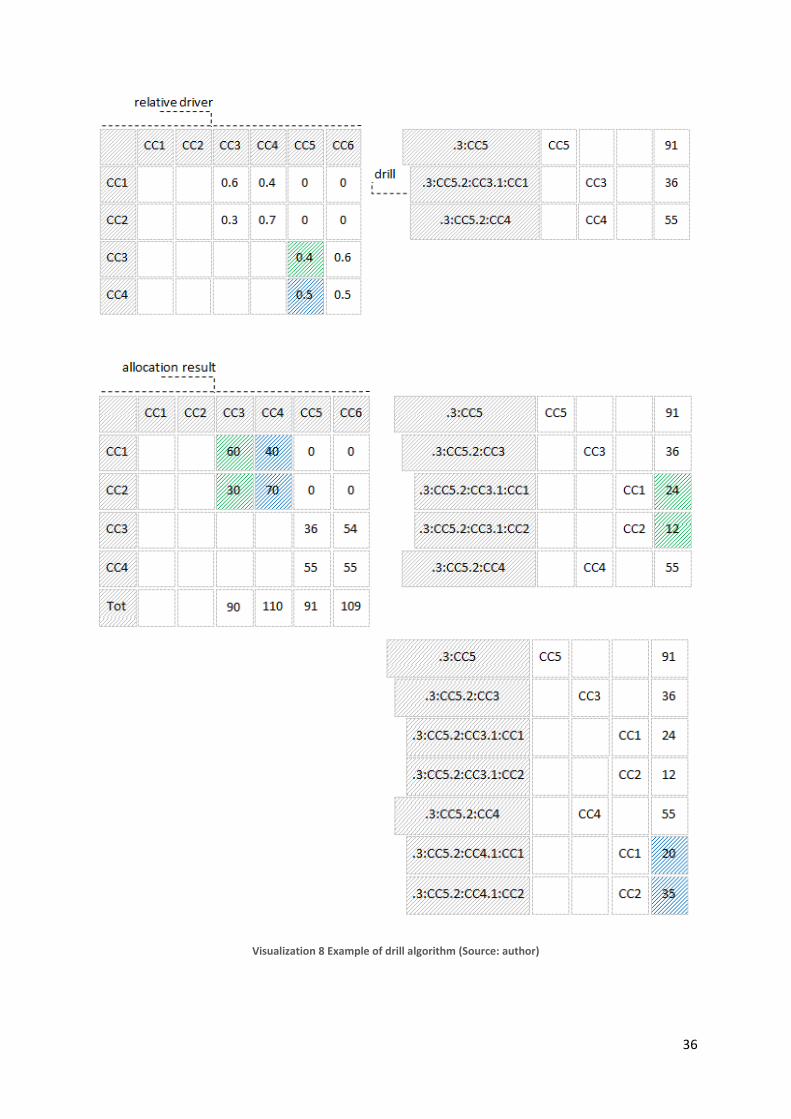
36
Visualization 8 Example of drill algorithm (Source: author)

37
Second structure of the standard allocation view sliced through allocation results in the visualization
8 suggests existing problem with inter-step aggregation. Cost centers CC1 and CC2 allocate
separately to cost center CC3 (60 units and 30 units), these are however sequentially consolidated
and allocated further to cost center CC5 as single value. When analyst is asked to provide
information about cost flow to fifth cost center, she is able to identify 36 units arrived from cost
center CC3, however any further composition is lost due to the inter-step aggregation. OnDemand
algorithm solves the problem by inverting the operations. For the purpose of explanation, allocator is
in the state depicted on first structure in right column. Analyst asks to drill second row in order to
find sources for the trace represented by the element code and marks it as drillable. While the value
36 is calculated by multiplying aggregated value 90 with driver on cost centers CC3 and CC5
intersection, the decomposition will be carried out by the same operation for every part of
aggregation. All parts of the aggregation can be found in the column under CC3 element in the
allocation result slice. Algorithm searches through the whole column of the target element and looks
for values different from zero. When such a source cost center is found, following two operations are
executed:
1. New record with unique trace code in vertical dimension is created by merging parent code with
source center name prefixed by its level in agreed notation. The record is then integrated into
existing hierarchy under its parent trace.
2. Amount for the new record is calculated by multiplying corresponding source center value and
target driver found on cost centers CC3 and CC5 intersection. Result is stored in the tablespace.
As presented in the example, it is obvious that algorithm runs into two non-zero values (highlighted
by green pattern) while searching appropriate column. Subsequently two new records will be
established in the onDemand table space and final results will be calculated. For cost center CC1
branch, the right portion is 24 units (60*0,4) while cost center CC2 represents 12 units (30*12). Same
sequence of operations can be used for drilling cost center CC4 in the third structure. Responsive
values are highlighted by the blue pattern.
From the previous description, whole algorithm can be summarized in following three steps:
1. Store driver value to the variable.
2. Search all columns under target center element for non-zero values.
3. If non-zero value is identified, create new record and multiply corresponding amount by
driver’s variable.
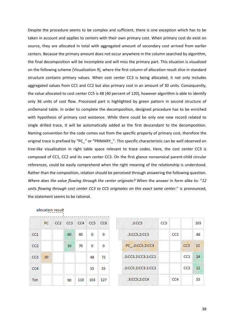
38
Despite the procedure seems to be complex and sufficient, there is one exception which has to be
taken in account and applies to centers with their own primary cost. When primary cost do exist on
source, they are allocated in total with aggregated amount of secondary cost arrived from earlier
centers. Because the primary amount does not occur anywhere in the column searched by algorithm,
the final decomposition will be incomplete and will miss the primary part. This situation is visualized
on the following scheme (Visualization 9), where the first column of allocation result slice in standard
structure contains primary values. When cost center CC3 is being allocated, it not only includes
aggregated values from CC1 and CC2 but also primary cost in an amount of 30 units. Consequently,
the value allocated to cost center CC5 is 48 (40 percent of 120), however algorithm is able to identify
only 36 units of cost flow. Processed part is highlighted by green pattern in second structure of
onDemand table. In order to complete the decomposition, designed procedure has to be enriched
with hypothesis of primary cost existence. While there could be only one new record related to
single drilled trace, it will be automatically added as the first descendant to the decomposition.
Naming convention for the code comes out from the specific property of primary cost, therefore the
original trace is prefixed by “PC_” or “PRIMARY_”. This specific characteristic can be well observed on
tree-like visualization in right table space relevant to trace codes. Here, the cost center CC3 is
composed of CC1, CC2 and its own center CC3. On the first glance nonsensical parent-child circular
references, could be easily comprehend when the right meaning of the relationship is understood.
Rather than the composition, relation should be perceived through answering the following question.
Where does the value flowing through the center originate? When the answer in form alike to: “12
units flowing through cost center CC3 to CC5 originates on this exact same center.” is pronounced,
the statement seems to be rational.
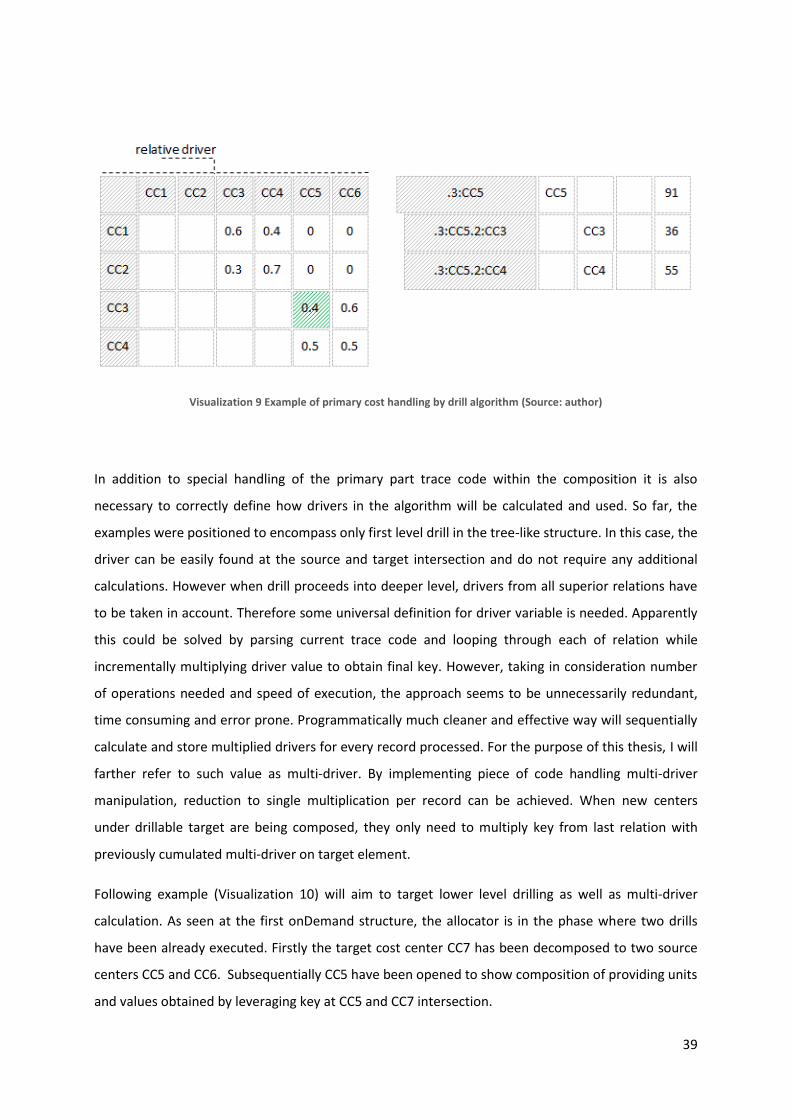
39
Visualization 9 Example of primary cost handling by drill algorithm (Source: author)
In addition to special handling of the primary part trace code within the composition it is also
necessary to correctly define how drivers in the algorithm will be calculated and used. So far, the
examples were positioned to encompass only first level drill in the tree-like structure. In this case, the
driver can be easily found at the source and target intersection and do not require any additional
calculations. However when drill proceeds into deeper level, drivers from all superior relations have
to be taken in account. Therefore some universal definition for driver variable is needed. Apparently
this could be solved by parsing current trace code and looping through each of relation while
incrementally multiplying driver value to obtain final key. However, taking in consideration number
of operations needed and speed of execution, the approach seems to be unnecessarily redundant,
time consuming and error prone. Programmatically much cleaner and effective way will sequentially
calculate and store multiplied drivers for every record processed. For the purpose of this thesis, I will
farther refer to such value as multi-driver. By implementing piece of code handling multi-driver
manipulation, reduction to single multiplication per record can be achieved. When new centers
under drillable target are being composed, they only need to multiply key from last relation with
previously cumulated multi-driver on target element.
Following example (Visualization 10) will aim to target lower level drilling as well as multi-driver
calculation. As seen at the first onDemand structure, the allocator is in the phase where two drills
have been already executed. Firstly the target cost center CC7 has been decomposed to two source
centers CC5 and CC6. Subsequentially CC5 have been opened to show composition of providing units
and values obtained by leveraging key at CC5 and CC7 intersection.

40
In order to streamline and simplify multi-driver handling, additional three columns have to be
introduced to onDemand table space.
Driver column keeps the key from actual intersection of source center being processed
and its target unit. The value will also be use in multiplication with multi-driver.
Parent multi-driver holds the sequentially cumulated percentage for the parent record.
The value is transferred from ancestor’s current multi-driver column and will also be
used in calculation of record’s own current multi-driver. This is the actual driver which is
used by algorithm to determine cost flow.
Current multi-driver is calculated by multiplying parent multi-driver with newly obtained
driver for particular record. The value will be used as parent multi-driver on lower level
of tree-like structure.
As explained in column definition, the driver actually used by algorithm is parent multi-driver. It is
also obvious that none of the columns have to by physically present in the table space and all
computing can be done through variables, however visibility of numbers can simplify validation and
debugging. For real implementation, only parent-multi-driver and current multi-driver are used in
form of actual columns.

41
Visualization 10 Example of driver calculation within trace cube
Current chapter defined objects and general algorithms required for successful implementation of
reengineered allocation model. In the following paragraphs, techniques and scripts used to develop
onDemand structure in IBM Cognos TM1 software will be presented. Additionally, server will be
extended with prepared procedures necessary for further extension with custom API.
3.7. onDemand Allocator solution implementation
Following paragraphs focus on explanation of tangible implementation in selected OLAP software
IBM Cognos TM1. The advancement in approaching particular objects corresponds with consecution
selected during concept introduction. Complete transcript of particular rules and processes can be
found attached in code snippets of Appendix A.
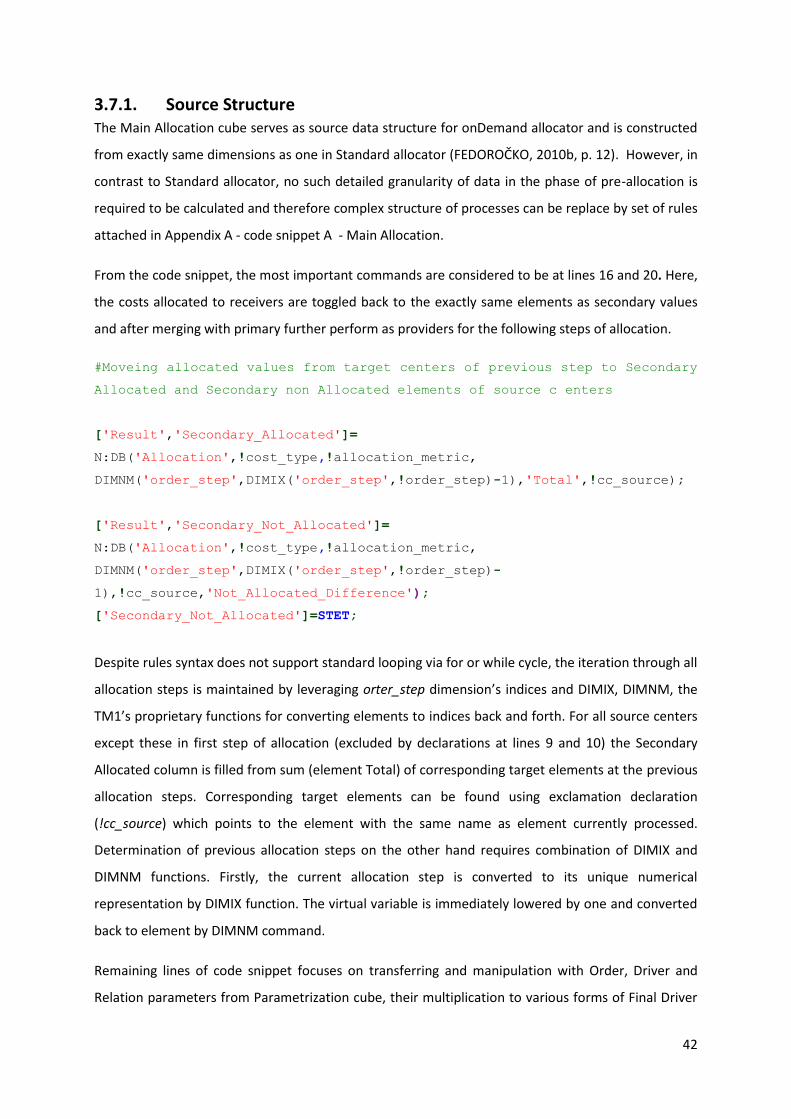
42
3.7.1. Source Structure The Main Allocation cube serves as source data structure for onDemand allocator and is constructed
from exactly same dimensions as one in Standard allocator (FEDOROČKO, 2010b, p. 12). However, in
contrast to Standard allocator, no such detailed granularity of data in the phase of pre-allocation is
required to be calculated and therefore complex structure of processes can be replace by set of rules
attached in Appendix A - code snippet A - Main Allocation.
From the code snippet, the most important commands are considered to be at lines 16 and 20. Here,
the costs allocated to receivers are toggled back to the exactly same elements as secondary values
and after merging with primary further perform as providers for the following steps of allocation.
#Moveing allocated values from target centers of previous step to Secondary
Allocated and Secondary non Allocated elements of source c enters
['Result','Secondary_Allocated']=
N:DB('Allocation',!cost_type,!allocation_metric,
DIMNM('order_step',DIMIX('order_step',!order_step)-1),'Total',!cc_source);
['Result','Secondary_Not_Allocated']=
N:DB('Allocation',!cost_type,!allocation_metric,
DIMNM('order_step',DIMIX('order_step',!order_step)-
1),!cc_source,'Not_Allocated_Difference');
['Secondary_Not_Allocated']=STET;
Despite rules syntax does not support standard looping via for or while cycle, the iteration through all
allocation steps is maintained by leveraging orter_step dimension’s indices and DIMIX, DIMNM, the
TM1’s proprietary functions for converting elements to indices back and forth. For all source centers
except these in first step of allocation (excluded by declarations at lines 9 and 10) the Secondary
Allocated column is filled from sum (element Total) of corresponding target elements at the previous
allocation steps. Corresponding target elements can be found using exclamation declaration
(!cc_source) which points to the element with the same name as element currently processed.
Determination of previous allocation steps on the other hand requires combination of DIMIX and
DIMNM functions. Firstly, the current allocation step is converted to its unique numerical
representation by DIMIX function. The virtual variable is immediately lowered by one and converted
back to element by DIMNM command.
Remaining lines of code snippet focuses on transferring and manipulation with Order, Driver and
Relation parameters from Parametrization cube, their multiplication to various forms of Final Driver

43
and subsequent allocation expressed as fold of Final Driver and Total Cost. More information about
Order, Driver and Relation parameters and semaphore technique can be found in Allocation
methodology (FEDOROČKO, 2010b, p. 14).
3.7.2. Trace Cube Trace Cube is the target structure of onDemand allocator and has been already introduced in
theoretical part. While the vertical trace dimension will be completely composed on the fly as analyst
determines in each step, the horizontal metric dimension comprises of three groups of elements:
Control elements
o Solve
o Drill
Auxiliary and final results elements
o Primary Value
o Value
o Current multi-driver
o Parent multi-driver
o Final Cost
Visualization elements
The concept of the first two groups has been already suggested in the theoretical section of
onDemand allocator. Whereas no rules are applied to these elements and their space is leveraged
purely by processes, elements will be references further in processes code snippets.
The third group of elements is designed to transform user unfriendly trace codes into tree-like
structure, where names of centers and their hierarchical position are easy to understand. The notion
of this intention could be easily comprehended for example from visualization 7 at page 34. It is
obvious, that number of elements will depend on number of possible hierarchical levels and it
simultaneously depends on number of allocation steps. Naming convention for elements was
selected to reflect the level of tree-like structure and therefore comprises of integers suffixed by
capital L. Despite, allocation steps is a variable metric, I decided to hard-code nine levels into metric
dimension for demonstration purposes. However, it could be easily replaced by process populating
trace metric dimension based on number of allocation steps.
Population of particular cells with names parsed from trace code is handled by command from code
snippet B – Tracing. The single prerequisite for the command to work universally is the equal length

44
of every cost center name including primary prefix. Therefore every part of the trace code in the
sample is exactly seven characters long and comprises of three characters long prefix of level
separated by dot and colon and four character long names. The code itself compares length of each
trace code with level and if equals, the proper part of trace code is inserted. For example, if trace
code is 21 characters long, then the name ought to be placed into the third level.
#Calculating Final Cost as Driver and Value multiplication
['Cost']=N:['Secondary_Driver_Parent']*['Value'];
#Every part of the !trace element identifying one cost center is exactly 7
characters long (including PRIMARY)#If the length of the !trace divided by
7 is same as column representing level, then last 7 characters (cost center
name) are inserted into proper cell
[]=S:IF(STR(LONG(!trace)/7,1,0) @=
SUBST(!trace_metric,LONG(!trace_metric),1),SUBST(!trace,LONG(!trace)-
3,4),CONTINUE);
3.7.3. Advanced trace visualization Visualization and presentation form of the solution is one of the most crucial factors when deciding
about success of the whole project. It is particularly customer need which has driven me to develop
custom TM1 API in order to be able to design advanced visualizations. However, with regard to these
needs and to table space restrictions TM1 provides, it is possible to simulate some of the advanced
presentations directly in cube slices. Especially for these purposes, the addition Tracing cube has
been introduced. It is necessary to highlight that the cube itself does not anyhow calculate or
contribute to onDemand allocation process and its single purpose is to transform existing trace codes
and hierarchies into more readable outputs while leveraging level structure added previously into
trace_metrics dimension. The two additional outputs are
Complete cost flow at cost center level
Complete cost flow at step level
In this context, term complete can be understood as extended trace code where information about
position of the allocated value at every level is maintained. Set of rules required for advanced
presentation is attached in code snippet C – Advanced Tracing.

45
3.7.4. Processes Processes of onDemand engine can be divided into three subject oriented groups
Initialization processes
Allocation processes
API processes
3.7.4.1. Initialization processes
Initialization processes focus on solution maintenance and are designed to automatically set up
allocator to its original state. While the only change during every analysis is incremental growth of
trace dimension, procedures have to firstly remove all elements and subsequently, according
selected target center, insert root element to the tree-like structure. Codes of both sub-processes are
attached in code snippets D and E.
3.7.4.2. Allocation processes
Allocation process has to be run every time analyst requires drilling selected nodes. The term drill in
the context of onDemand allocator was already introduced in theoretical section at page 35 and
therefore the focus in this part will be placed exclusively on its algorithmic representation. While the
analyst is able to identify multiple nodes to be drilled between allocation circles, procedure has to
loop through all existing nodes in the trace dimension and searches for occurrences, where both Drill
and Solve parameters are assigned Boolean 1. When such a node is found, the following operations
have to be executed:
Add new elements under drilled node in trace dimension.
Search and calculate auxiliary parameters and final results for every new element.
While the logic focuses on two different TM1 objects and separates them into two standalone blocks,
the implemented sub-processes will also follow this notion. Therefore, the dimension handling will
be implemented in crawlElement process, while value manipulation will be supported in crawlValue
procedure. The code for root allocation process executing both process is attached in code snippet F.
Whereas all non –target centers are potential sources for drilled node, the procedure receives their
subset on input and further searches in pre-allocated values of Allocation cube to filter relevant
candidates.
The traceElement code transciption can be found attached in code snippet G. The lines with required
attention are listed in the table below (Table 8). Before proceeding to the code, it is also necessary to

46
highlight, that in order to keep implemented processes as simple as possible, the cost type dimension
have been skipped and explicitly set to first element in both processes. When any additional
dimensions would be desired to be added into processes, the input view as well as particular queries
would need to be adjusted appropriately.
Table 8 Query explanation of significant lines - procedure crawlElement (Source: author)
Line # Query Explanation
29 Inserting primary element as part of every drilled node
49 Receiving appropriate value from source structure
55 Condition allowing further processing only for non-zero values having the allocation relation
68 Constructing unique trace code
73 Adding trace code into the trace dimension
The core concept behind the crawlValue procedure is similar to previous one, however focuses on
values processing instead of elements. Therefore, the input data in form of all non-target centers
subset and their subsequential filtering is kept unchanged. The code transcript is attached in code
snippet H and explained in the following table (Table 9).
Table 9 Query explanation of significant lines - procedure crawlValue (Source: author)
Line # Query Explanation
14 Executing crawlElement procedure from within itself
18-21 Transfering and storing values and drivers from already drilled ancestor
39 Condition allowing further processing only for non-zero values having the allocation relation
59 Loading primary cost for currently processed unit
64 Loading driver for currently processed unit
68 Calculating new driver
81-85 Setting Solve parameter for non-primary units
3.7.4.3. API processes
Except core processes necessary for onDemand allocator implementation in TM1, the server has
been extended with set of auxiliary procedures which will be leveraged further when creating custom
API.
While the notion behind Application Programming Interface is possibility to execute basic input and
output operations from outside the TM1 environment (SPOFFORD, 2006, p. 46), processes focus
mainly on setting parameters and exporting demanded views. Overview of their purpose is attached

47
in table 10 while specific meaning will be referenced further in the thesis, when the different parts of
API are being developed.
Table 10 Explanation of particular API processes (Source: author)
Process Purpose explanation
Set Drill Enables remote selection of node to be drilled via trace code. Sets particular Solve parameter to one.
Set Center Enables remote selection of target center to be drilled.
Create Selection Runs process generating subset of target centers offered in target center selection.
Treace Export Exports subset of trace codes and values created in last drill in JSON format.
Selection Export Exports subset of target center for initial selection.
Reset Export Exports single line of root trace code and its value.
So far the thesis has introduced current cost allocation model in IBM Cognos TM1, analyzed its
weaknesses and problems as well as designed novel onDemand solution under the hypothesis of all
obstacles removal. Having the reengineered model implemented it is necessary to compare it to the
original structure and validate outspoken premises. The following chapter therefore presents
researched literature focusing on OLAP models benchmarking, develops own adjusted framework
and analyzes results of conducted researches and measurements.

48
3.8. Standard vs. onDemand solution benchmarking
The impulse for allocation reengineering arose from set of known issues which have been collected
from customers and partners feedback during more than two years of original model existence
(BOTHE, 2010; BOTHE, 2011). These arguments, discussed in the standard allocator issues (page 19),
are considered to be the wall stones of the entire onDemand solution and consist of:
Speed of calculation
Volume of generated data
Tracing capabilities of cost flow
Interpretation and visualization of results
Complexity of rules and processes
In order to be able to reliably prove, that newly proposed concept removes every obstacle affiliated
with standard allocator, the analysis as well as benchmarking of both models has been conducted. So
far, the introduced concept has confirmed solely the possibility to improve and particularize tracing
capabilities, however sufficiently has not yet addressed remaining objections. The following
benchmarking therefore places the biggest importance on residual factors including performance
metrics, usability and development severity.
In current section I will initially justify four perspectives that have to be taken in account when
assessing allocation models and subsequently nominate set of metrics which will be benchmarked in
every category. After the metrics definition, detailed methodology and approach to evaluation of
each metric will be presented. Quantitative and qualitative goals determining fulfilment in every
category have been set before implementing the pilot solution and will be published before I
proceed to solitary measurement and benchmarking. In conclusion, I will evaluate and compare
actual results to specified goals as well as draw final effects and consequences.
3.8.1. Benchmarking metrics definition Four perspectives taken in the account during benchmarking emerged from industry’s standards and
best practices. The basis for the framework has been found in the OLAP Council initiation APB-1
which constitutes set of measures designed to distinguish performance deviations of various OLAP
software (OLAP COUNCIL, 1998, p. 3). It is obvious that whereas both models run on the exactly same
infrastructure, some metrics will account equal results. However factors such as speed, number of
queries executed and volume of data will be significantly influenced by the preciseness of the

49
implementation. While these measures align smoothly with first two objections and are able to strictly
mirror the performance contrasts, they will be applied in the constructed framework under
performance perspective. The performance perspective is however not enough for complex
measurement of software quality what is reflected by origination of various norms and standards
offering more advanced and diverse view. The ISO/IEC 25000 introduces six key dimensions, which
focus not only on performance, however also on usability, functionality and maintainability of the
solution (ISO/IEC 25000, 2005, p. 10). These additional factors correspond well with proposed
arguments and are therefore ideal for extending developed framework. The maintainability of
software will be for benchmarking purposes further enhanced to development and maintenance
perspective. This perspective focuses on benchmarking difficultness and agility to develop particular
model as well as its further maintainability and ease of implementing extensions. On the other hand,
the ability to adopt the solution, its intuitiveness and anlyst’s overall satisfaction will be taken in
account during qualitative assessment of model’s usability. For the purpose of qiving this soft, however
important metric tangible value, the speed of analysis execution and agility to react to various tasks will
be empirically measured. Eventually, collected data will be enriched with their monetary evaluation
and materialized into single business metric expressing the financial expensivness of developing,
operating and maintaining such solution. The final framework therefore comprises of:
Performance perspective
Development and maintenance perspective
User experience perspective
Business and financial perspective
3.8.1.1. Performance perspective
Performance perspective was selected to address issues linked to speed of execution and volume of
generated data. Taking a deeper look, several important factors influenced by these measures can be
found. Firstly, speed and volume is tightly related to hardware infrastructure, where significant
savings can be made by reducing required performance. Additionally, speed of operation and time to
result for ad hoc analyses can affect number of executions per time period and therefore influence
overall quality of attained conclusions. Eventually, volume of redundant data has also impact on
executed analyses. With increasing fruitlessness, results become more difficult to read, orientate and
search in, what subsequently affects not only promptness of work however again the ability to obtain
the most accurate effects.
The only way how to precisely measure performance is by empirical experiments. Therefore both
engines need to be set up and tested at the available infrastructure while the observed values are

50
collected from logs or appropriate files. However, the single measurement of the performance will
not be sufficient and will not satisfactorily reflect contrasts in models under various setups. Firstly it
would not be enough to assuredly draw conclusions as well as on the other hand would not reveal
dependences between performance and settings needed to make further recommendation about
proper system in particular conditions. In order to observe performance characteristics as precisely
as possible, every metric has to be captured and compared for engines with variable number of cost
centers and allocation cascades.
With two performance objections in mind and expectation of significant variances in results, the
most appropriate factors available to measure can be found within set of strict metrics from APB-1
framework which is for a long time considered to be standard among OLAP vendors. Despite few of
them loose relevance when benchmarking is execute on identical system, remaining sufficiently
cover question of execution speed and volume of generated data. The selected measures include:
Average volume of generated data
Average time of execution
Time to result
Processor utilization peaks
RAM memory consumption peaks
The output of the simulations then generates performance matrix including various setups on
vertical dimension and observed factors in columns. Based on this concentration, various absolute
and relative comparisons can be executed as well as dependency between settings and appropriate
model can be deduced.
3.8.1.2. Development and Maintenance perspective
The perspective has been integrated into the benchmarking framework because of the huge impacts
architectural concept and development severity can have on numerous factors subsequently
influencing the overall viability (COSTEA, 2007, p. 98). Firstly, the magnitude of development efforts
expressed also as a size of the project can be directly mirrored to financial metrics. In addition the
software complexity, defined as the degree to which the implementation is difficult to understand,
hence develop (KEARNEY, 1986, p. 1044), also indirectly transfers into future maintenance and
upgrade expenditures. Eventually the size of the solution determines extensions and modifications
agility. Taking in consideration floating conditions and continuously altering environment in the
organizations, it is crucial for allocator to have lower possible complexity allowing rapid transition
with minimal overheads.

51
Extensive research proved that there does not exist specific metrics for assessing severity of OLAP
model. However, the complexity of general software is heavily discussed topic with long history of
research (KEARNEY, 1986, p. 1044; MISRA, 2008, p. 1691). Taking in consideration numerous
similarities between object oriented and OLAP programming it is obvious that these factors could be
transferred and applied also to OLAP engines. Mentioned parallels would link objects to cubes, their
attributes to dimensions and methods to ETL processes. Several authors propose variety of equations
which can be extracted and concluded into framework best fitting specific environment
characteristics. In order to keep metric simple to comprehend, frugal to calculate and easy to
compare, I decided to materialize model complexity into single variable. Despite it may seem
insufficient, variable covers almost all aspects determining magnitude of expended efforts.
Since OLAP cubes are considered to be main building blogs of every model, the overall complexity
(Mcom) will be calculated as sum of their fragmental complexities (Ccom).
∑
This singular value can be further decomposed into complicacy of its rules and processes. While
development severity of rules depends directly on number of dimensions treated, the multiplications
between lines of code and dimensions count can be used. Additionally cubes are operated by set of
input and output processes, those complexities can be expresses by number of generated or
manually embedded lines of code multiplied by dimensionality of its input cube.
∑
Final complexities are presented in the following paragraph and include their absolute values as well
as relative comparisons.
3.8.1.3. User Experience Perspective
Ways how software is visually designed and appealing to end user plays important role in its overall
quality. This applies even more when its purpose is to analyze data and present challenging relations.
Seffah (2006, p. 160) declares, that usable interface accounts for several observable benefits. They
range from performance improvement and productivity through security and overall popularity to
commercial viability. This is however proved not only empirically, but numerous norms and
standards such as ISO/IEC 9126-1 (2001) or IEEE 1061 (1998) standard (Software Quality Metrics

52
Methodology), include usability attribute in their roots for evaluating software quality (SEFFAH, 2006,
p. 161). Third justification of user experience perspective in designed framework refers to the
outspoken objection pointing to the poor presentation capabilities in standard allocator. Purpose of
the perspective therefore lays on validating hypothesis of improved readability by implemented
alternative.
Seffah (2006, p. 161) and Fitzpatrick (1998, p. 5) developed set of tactics how to measure software
usability based on acknowledged and previously successful methods. Both composites derive from
industrial standards listed above or from previously acknowledged works of authors such as Dix,
Nillsen and Preece. These proven frameworks propose wide variety of techniques ranging from
simple ones such as interviews and questionnaires to complex observations with presence of
psychologists and expert groups. Taking in consideration attainable range of possibilities I decided to
guide my selection based on the availability of resources and actual goals I intended to observe.
Goals include:
Ability to obtain desired information in the shortest possible time and with minimal errors
Possibility to read and understand presented data and relations
Independency in basic modifications and parameters setups
Significant focus on user in all these three tasks suggests, that interviews and empirical measuring
among large diverse group of participants will be appropriate for determining effects. Based on these
findings, small research was conducted in October 2012. The research was hold in Prague, Czech
Republic and included sample of participants with different experience and knowledge of the topic.
The interview comprised of theoretical part during which interviewee was introduced to the
allocation concept and familiarized with the different interfaces and empirical observation when I
assigned analytical task and measured time to resolution and number of dispensable steps.
Subsequently I asked participant for qualitative assessment of intuitiveness level and ease of use. The
findings of the research are presented in the particular section of results paragraph (p. 58).
3.8.1.4. Business and financial perspective
During the research of numerous performance evaluation methodologies, software complexity
framework or usability tests, I have met only minimal evidence of financial factors or attempts to
assign quantitative monetary effects to observed facts. However, on the other hand I feel that
especially this should be one of the goals for both implementation provider as well as potential
customer when looking for alternative solutions. Although it does not mean that entire evaluation
should be diminished to single value, the presence of this factor in software selection procedure as
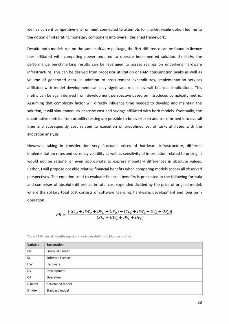
53
well as current competitive environment connected to attempts for market viable option led me to
the notion of integrating monetary component into overall designed framework.
Despite both models run on the same software package, the fisrt difference can be found in licence
fees affiliated with computing power required to operate implemented solution. Similarly, the
performance benchmarking results can be leveraged to assess savings on underlying hardware
infrastructure. This can be derived from processor utilization or RAM consumption peaks as well as
volume of generated data. In addition to procurement expenditures, implementation services
affiliated with model development can play significant role in overall financial implications. This
metric can be again derived from development perspective based on introduced complexity metric.
Assuming that complexity factor will directly influence time needed to develop and maintain the
solution, it will simultaneously describe cost and savings affiliated with both models. Eventually, the
quantitative metrics from usability testing are possible to be overtaken and transformed into overall
time and subsequently cost related to execution of predefined set of tasks affiliated with the
allocation analysis.
However, taking in consideration very fluctuant prices of hardware infrastructure, different
implementation rates and currency volatility as well as sensitivity of information related to pricing, it
would not be rational or even appropriate to express monetary differences in absolute values.
Rather, I will propose possible relative financial benefits when comparing models accoss all observed
perspectives. The equation used to evaluate financial benefits is presented in the following formula
and comprises of absolute difference in total cost expended divided by the price of original model,
where the solitary total cost consists of software licencing, hardware, development and long term
operation.
| |
Table 11 Financial benefits eqution's variables definition (Source: author)
Variable Explanation
FB Financial benefit
SL Software licences
HW Hardware
DV Development
OP Operation
D index onDemand model
S index Standard model
54
3.8.2. Defined goals Current paragraph will state partial goals as well as the overal criteria assigned to individual
perspectives in order to determine viability of onDemand allocator design and implementation.
These target values will be compared to actual results collected during following benchmarking and
experiments as well as used in the conclusion of the chapter to evaluate desired effects. Taking in
consideration disproportion of generated cost flows by the onDemand allocator in contrast to
original model, it would be sufficient if 50% decrease in speed of execution and 25% contraction in
performance consumption were achieved. Considering the development and maintenance
perspective, the implementation complexity factor is desired to drop at least by 30%, what would
significantly influence time and resources required to deploy the functional application. Additionaly,
the prevailing positive feedback from interviewed participants acompanied by 40% decline in single
average analysis time is required to declare the interface usability as sufficiently improved.
Eventually the demanded financial benefit from onDemand deployment and operation is defined to
be at minimal 30%. Taking in consideration all perspectives, the benchmarking of novel approach will
be perceived as successful and will confirm hypothesis about possible removal of existing issues and
obstacles affiliated with original model, if at least three of four perspectives outputs satisfactory
results.
3.8.3. Benchmarking Results
3.8.3.1. Performance perspective
The measurement was conducted on virtualized 64bit Windows 7 operation system with dedicated
4GB of RAM memory and Intel Core Duo with 2.8 GHz. Both servers of IBM Cognos TM1 installation
were in 10.1.0 version.
For the purpose of testing engines under various conditions, 60 measurements in total with 12
different setups have been executed. Setups were divided into two pools with five and ten allocation
steps while in every pool gradually the allocation performance over 80, 240 and eventually 480 cost
centers was tested. Despite in practice, even larger sets are common, hardware restrictions did not
allow to benchmark wider models. Additionally, in order to capture effects of different cost centers
to allocation steps assignation patterns, each model setup was run twice. Firstly, the equal
distribution of cost centers was used while during second run number of cost centers in last steps
was doubled.
55
These twelve measurements were repeated five times. First two focused on full allocation in
standards and subsequently onDemand model. Full in this particular context means processing of
each cost from every cost center and simultaneously identification of every possible cost flows to all
receivers. While for standard concept the full allocation is common practice and cannot be anyhow
restricted, in onDemand it requires gradual selection of target centers and their subsequent drilling
to the lowest possible level. Remaining three measurements targeted ad-hoc capabilities. Similarly,
ad-hoc in the allocation context refers to random selection of cost flow trace according analyst
requirement and its resolution. Whereas the standard models is not capable of ad-hoc querying and
desired traces have to be eventually located within full load sets, the examined metric will need to be
taken over from general performance results. On the other hand onDemand support of ad-hoc
exploration enabled its benchmarking which was separated into tree standalone cycles differing in
drill depth. Continuously I simulated analyst behaviour tracing cost flow to 1/3, 2/3 and 3/3 of the
actual trace length. It means that for ten steps allocation, first exploration drilled only three levels
down while during the last one, the lowest possible level was reached.
With each measurement, five observed metrics have been recorded. For hardware performance
benchmarking, Windows intrinsic Performance Monitoring Tool collected statistics about average
and maximum percentage of processor time consumed. The total run time of allocation process was
engrafted in TM1 Message log file. Additionally, overall number of generated traces could have been
manually calculated from cubes with each of dimension nested into horizontal axes. Eventually RAM
memory utilization corresponding to volume of data contained in main allocation cube was hand-
taken from particular file on file system after its storing to computer’s hard disc.
Granular records are attached in Appendix B. First table Hardware Performance – CPU documents
processor’s average and maximal utilization during six different setups of equally distributed cost
centers for both standard and onDemand concepts. Firstly, it is important to notice that while
utilization of standard model growths steadily in range of 6 to 15% with increasing size of
dimensions, the onDemand accounts erratic behaviour. Further examination of generated results
after each round revealed, that overall utilization will likely depend on average number of child
nodes opened with single drill. While in shallow hierarchies (small sets of child elements) engine
executes more less demanding crawling operations, deeper structures require increased
computation power. This hypothesis could be also confirmed from comparison of average utilizations
in five and ten step setups. It is obvious that in the ten steps setup, only half of cost centers are
assigned to particular steps when comparing to the five cascades. Therefore, also drilled hierarchies
are supposed to be more shallow and less performance demanding. The actual averages scored 53.1
% for five steps while only 42.6 % for double cascades what accounts for 19.7 % utilization decrease

56
and therefore confirms the theory. From overall performance benchmarking, standard models
consumes at a medium 54.5 % of processor time with peaks at 96.2 % while onDemand leverages
only 47.8 % and in average reaches 71.7 % of total computation power. Collected results suggest that
the reengineered model is 12.1 % more efficient and could reliably operate on machine with ¼ less
processor power then original concept.
For the purpose of actual algorithm performance benchmarking, I decided to separate and
independently compare results for full and ad-hoc models. This notion emerges from attempts to
most precisely capture two types of scenarios allocators is designed to and simultaneously even in
the bigger detail identify potential differences.
Complete documentation of Full load results is attached in Appendix B under title Algorithm
Performance – Full Load. Similarly, twelve settings were used for which I recorded number of traces
generated, speed of execution and volume of memory occupied. Although it may seem from
absolute values that onDemand allocator accounts for far worse metrics in contrast to standard
concept and loose in every category, it is important to pay close attention to statistics about number
of rows generated. While in onDemand allocator, number of calculated traces Td could be easily
deducted from dimension keeping every unique trace code, the standard allocator does not offer any
means how traces could be identified. However, it is possible to use simple equation to determine its
feasible count. Equation leverages number of allocation steps S and count of cost centers assigned to
last cascade F.
When comparing TD to Ts in general, it is obvious that significant irregularities between both models
occurred and therefore comparison in absolute values would not be relevant. Additionally, when
observing five and ten cascade clusters separately, it reveals that whereas in ten steps 8 to 25 times
more traces are generated, in the half one, the multiplicator is extremely higher (250-2000). This is
caused by two factors. Firstly, in standard concept, Ts equation returns much more possible
combinations for ten cascades. Simultaneously for the same setup, shallow dimensions in onDemand
model are able to generate fewer traces. Taking in consideration identified irregularities, much more
appropriate overview therefore offers recalculation of both metrics to single unit of trace. These
relative proportions VT and ST are captured in last two sub-tables of Algorithm Performance – Full
Load. Based on the percentages, two facts need an attention. Firstly, increased number of cost units
in last cascade plays into the hands of standard allocator. While onDemand concept is irrelevant to
number of units in last cascade, standard model accounts better relative results the higher is the
distribution in last group and therefore also more satisfying outcomes when comparing to its
57
counterpart. Secondly, taking in consideration overall performance, onDemand concept improved
averaged volume of memory required for single trace record by 22% from original 0.105 to 0.081 kB.
Even better results were obtained for speed measurement where onDemand concept decreased
time required for calculating unique cost flow by 65 % from 0.051 to 0.018 second.
Whereas onDemand allocator has been reengineered with emphasise on improved user control
during allocation process, even better results have been expected from ad-hoc benchmarking. My
intention was to measure time to result indicator, which reveals how much time it takes analyst to
find required information. The information can be searched either knowingly with purpose to
identify quantity at selected node in specific level or unconsciously by drilling suspicious nodes based
on observed anomalies. In addition to time I also recorded number of rows which need to be
generated and stored in memory during single ad-hoc query. Traditionally twelve different setups
were used, while this time every setup was subjected to three ad-hoc analyses differing in examined
depth. Ad-hoc queries were executed continuously to search for information in 1/3, 2/3 and at the
end of the trace. Whereas standard model does not support graduate definition of required data,
complete execution of allocation is needed prior to its subsequent filtration. Therefore, every record
for standard concept was taken over from full load statistics. As follows from Algorithm Performance
– Ad-hoc table documented in Appendix B, onDemand engine achieved 95.6 to 97.3 % improvement
in speed of execution while simultaneously 88.5 to 94.2 % of generated data was saved.
Based on defnied goals, it is obvious that reengineered approach met the dedicated target of 50 %
decrease in allocation speed and simultaneously consumed approximately 25 % less of computing
power.
3.8.3.2. Development & maintenance perspective
For the purpose of model complexity index calculation, several parameters from both servers had to
be collected and subsequently embedded into prepared formulas. Complete documentation of
assembled values is listed in Model Complexity table of Appendix B. It is necessary to highlight, that
few modifications were taken in account with aspect of avoiding potential distortion. Firstly, on a
cube level I excluded data preparation modules such as Driver, Relation or Parameterization while
they were indispensable components but could have had diverse implementation. Additionally, some
redundant dimensions providing extended view on data were omitted from core cubes and only
necessary one, introduced in previous chapters, have been left in. Among rules, merely these,
actually processing data were count while nested conditions were always considered as single lined.
Eventually, same applied to processes where auxiliary constructions such as loop structures or
attribute and subset handling prepared for API were also bypassed. Although the equation

58
determined onDemand concept complexity to 246, 57.8 % of development and maintenance effort
has been saved comparing to original standard model’s complexity index assessed to 584 points. As
reasoned in development and maintenance methodology, this saving has impact not only on initial
implementation phase however also on future modifications and extensibility.
When assessing the obtained results, it is possible to declare onDemand allocator to be successfully
complaing also the defined goal of the development and maintenance perspective.
3.8.3.3. Usabilityperspective
Despite intervieved participants differed significantly in age, level of achieved education, profession
and experience with cost allocation topic, very similar features have been identified in both
qualitative and quantitative parts of conducted interviews. From the qualitative dimension the
experiment focused not only on intuitiveness, comfort and overall satisfaction with user interface,
however also on speed of adoption with analytical process in particular model during time. With
intention to identify the velocity and level of advancement penetration, interviewees were
repeatedly asked to conduct the analysis and solve specific tasks. Initial results were suprising and
slightly disappointing. While not only a single temporary analyst has any problems with identifying
required values in standard allocator, majority of participants have struggled to find a proper
numbers in onDemand approach and eventually faild to provide satisfactory answers. The reson was
in most cases caused by misunderstanding the concept of tree-like structure and its reverse fashion.
However, with the additional explanation and highlighting of core onDemand concepts as well as
suggestions how to approach the analysis after the first attempt, collected data and participants
feelings have significantly changed immediately during second set of tasks. While their approach to
standard allocator has not change afterwards, the mastering of tree representation could have been
observed with every additional task. Eventually, all participants reported that despite standard model
seemed to be simplier and more intuitive at the beginning, it later turned to be ineffective,
longwinded, indecipherable, and hard to search in. On the other hand, initial confusion and aversion
to onDemand allocator quickly disappeared as participants adapted to the conpcet, its structure and
different way of perceiving data then common table space representation. Finally, interviewees
praised new approach to be easier to read, operate and manipulate while simultaneously mitigates
risk of making unnecessary errors. Moreover they confirmed that such presentation of information
and their relations makes more sense as well as noticed that data are provided in bigger detail than
these from original model, what simulatenously decrese effors put into further processing. From
quantitative perspective, participants were asked to assign single numeric grades on scale of 0 to 10,
based on their overall experience with presented interfces. The onDemand model received average
rating of 8.6, while the original approach finished with 4.5 points, what can be considered to be 91%
59
improvement in application usability. Furthermore, each of conducted analysis was accompanied by
precise measurement of time in seconds, revealing the required period for finding appropriate
information. Whereas the initial measurement finished in behalf of original approach because of the
significant distortion in onDemand model caused by numerous wrong or failed answers, the
subsequent rounds accounts for totally opposite findings. The analysis of selected trace took on
average only 3.8 seconds in tree structure, while the slicing throught particular steps of original
model consumed 12.4 seconds. Similar results have been obtained also in the last third assignment,
where onDemand times hovered around 4.2 seconds but standard approach to analysis kept the
required period unchanged.
In conclusion, the relative time savings recoreded during interviews and experiments fluctuated in
range of 60-70%, what is a result significantly overclasing the goal intended at the very beginning of
the benchmarking process.
3.8.3.4. Business and financial perspective
Althought final business metric is supposed to transform all previous perspectives into single, easily
perceived unit, it is obvious that with such a large number of unknown and variables, the predicative
value would not have a huge importance. Among the most distorting factors can be included actual
size and complexity of the solution, quality of project management and skills of implementing team
as well as the depth, frequency and difficultness of conducted analyses. Despite that, I attempted to
define set of assumptions to approximate implemented models to the reality and create exemplary
scenarios, in order to be able to come as close as possible to determination of relative financial
benefits provided by reengineered solution. Based on the conducted performance benchmarking,
the middle size model with 240 cost centers and 10 steps has been selected for software licencing
and required hardware estimation pricing. Additionally, the measured 25% decrease in performance
demand was taken in account to simulate expected savings. Considering development expenditures,
the calculated model complexities have been leveraged, while the estimated number of required
mandays has been obtained through my personal assumption of developer’s ability to solve in
average 24 complexity units per day. The costs affiliated with model operation and usage have been
extrapolated from performed interviews, expecting monthly period in conducting analysis over 24
target centers in fully-fledged middle size allocation models. Because of the volatility in exchange
rates and prices affiliated with variables used in the proposed equation, but mostly because of the
sensitivity of employed information, detailed calculations will not be published in this thesis.
However, based on my personal valuation from November 2012, the approximate savings affiliated
with exemplary onDemand model in contrast to standard allocator represented 23.9 %. Despite

60
obtained value did not completely fulfil defined goals but approached it very closely, it is possible
that some implementations in conforming conditions will reach desired level of savings.
So far, I have analysed and proposed specified framework for benchmarking two different OLAP
models built on the same software architecture. In order to touch every aspect of influence caused
by their implementation into enterprise environment, it comprises of four different perspecitves
including performance affection, development and maintenance severity, overall usability and
intuitivnes as well as consolidating financial and business implications. Within every dimension I
defined observed metrics and proposed practices and methodologies enabling viable evaluation of
their values. Before solitary benchmarking, every metric has been assigned a minimal target goal.
Based on the conducted benchmarking and research, the absolute fulfilment of almost all objectives
proved that reengineered solution successfully removes all obstcles and bottlenecks identified
durings initial analyses and moreover introduces tangible benefits affiliated with its preference over
standard methods.
61
4. Custom TM1 API and Advanced Visualization
Introduced native onDemand allocator partially solved objections of results readability and overall
usability. The tree-like structure proposed by Bordley (2002, p. 140) enables simpler interpretation
of cost flow due to flat space top down expansion and separation of particular levels to individual
cascades. Moreover, the usability improvements were recorded on analytical side where slicing and
dicing necessities of allocation cube were removed. On the other hand, the allocator operation was
limited to zero to one switching and single process execution. Despite it may seem as radical upgrade
and attainment of maximal capabilities OLAP space offers, some imperfection can still be found.
Firstly, the visual representation of results for perception and comparison purposes could be
improved by leveraging color schemas and radius scales as proposed by Mansmann (2007, p. 3). In
addition, the clarity of cost flow structure in very lager cubes can be diminished by wide gaps among
child and parent elements. The vertical structuring also makes it very difficult to compare two and
more adjacent flows. The solution can be found in more space conscious positioning of relevant
nodes. Eventually, even the simple zero to one switching and subsequent process execution doesn’t
meet standards of current applications and needs to be integrated into single command. It is obvious
that none of these arguments can be further eliminated purely by leveraging TM1 native
functionality. Despite, some issues can be mitigated by deploying allocator to MS Excel or reporting
interface, it would never solve everything at the same time.
Based on the deep research, advanced visualization can be solved by developing own and standalone
interface especially suited for tree structure representation of allocation results. Taking in
consideration web browser’s adoption as application interface, numerous languages, frameworks,
libraries for graphical visualization and animation (BARANOVSKIY, 2012; SHARP, 2010, p. 279) as well
as their conformity to integration services (LENGSTORF, 2010, p. 78), I decided to implement
allocator’s front-end using web technologies. Selected approach will also properly separate
application and presentation logic as visualized at the following image (Visualization 11). However
TM1 does not offer any convenient way how to integrate and access data from outside the set of
native interfaces. Despite introduction of simple API in version 9.5.2 (IBM, 2011a, p. 19), it is
restricted to accessing basic components and does not meet the complex requirements necessary for
communicating and operating implemented model. Clashing against this hurdle, I decided to conduct
extensive research and undergo TM1 numerous experimentations which aimed to prove the
feasibility of developing own custom API. Because of the positive outcomes, the following paragraphs
will focus on introducing architectural conception, best practices and techniques used during the

62
development. After the solitary API implementation, it will be used to design and demonstrate
different advanced visualizations analyzed in the last chapter.
Visualization 11 Separation of application and presentation logic and it’s integration (Source: author)
4.1. Custom TM1 API
Next paragraphs focus on analyses and design of core API components. API is defined as
an interface which is used for accessing an application or a service from a program. An API makes it
possible to use programs from within programs, therefore it is the foundation for modular systems
with clearly defined interfaces between separate components (MULLOY, 2012, p. 3). Whereas every
API communication is bi-directional and two separate systems are being connected, at least four
different logics need to be implemented.
The bi-directional communication means that there are two major problems which need to be solved
generally when designing APIs. How can application "request" the provider for specific data output?
How will the provider "respond"? On the other hand two separate communicating systems stand for
requestor and provider. The provider is in case of onDemand allocator represented by TM1 while
requestor will be implemented in web-based front-end interface. Overall structure of communication
cycle composed of four separate logics with techniques and ways of means can be observed on the
following visualization (Visualization 12). The logic consists of request invoking, request processing,
response formatting and response receiving, which are closely discussed in the next sections. In
order to keep the consistent understanding and alignment with the actual development steps,
particular components will be introduced gradually starting with back-end request processing in right
upper part of the visualization (Visualization 12) and continuing in the clockwise fashion to the front-
end invocation.
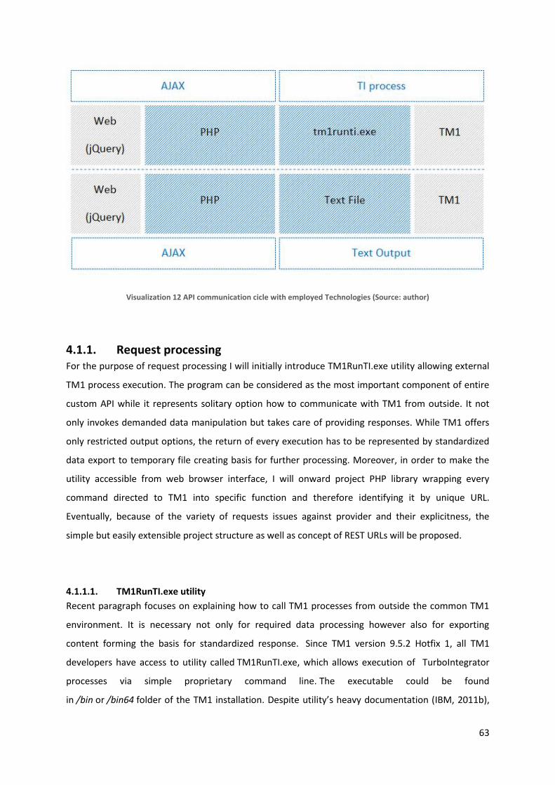
63
Visualization 12 API communication cicle with employed Technologies (Source: author)
4.1.1. Request processing For the purpose of request processing I will initially introduce TM1RunTI.exe utility allowing external
TM1 process execution. The program can be considered as the most important component of entire
custom API while it represents solitary option how to communicate with TM1 from outside. It not
only invokes demanded data manipulation but takes care of providing responses. While TM1 offers
only restricted output options, the return of every execution has to be represented by standardized
data export to temporary file creating basis for further processing. Moreover, in order to make the
utility accessible from web browser interface, I will onward project PHP library wrapping every
command directed to TM1 into specific function and therefore identifying it by unique URL.
Eventually, because of the variety of requests issues against provider and their explicitness, the
simple but easily extensible project structure as well as concept of REST URLs will be proposed.
4.1.1.1. TM1RunTI.exe utility
Recent paragraph focuses on explaining how to call TM1 processes from outside the common TM1
environment. It is necessary not only for required data processing however also for exporting
content forming the basis for standardized response. Since TM1 version 9.5.2 Hotfix 1, all TM1
developers have access to utility called TM1RunTI.exe, which allows execution of TurboIntegrator
processes via simple proprietary command line. The executable could be found
in /bin or /bin64 folder of the TM1 installation. Despite utility’s heavy documentation (IBM, 2011b),

64
none of the sources offers exemplary syntax for real life use and scenarios for different conditions.
Based on my research and experimentation, the mere examples have been firstly introduced in blog
post (FEDOROČKO, 2012a). The example of random request to run the test process with
parameter param and value p1 on demoserver as admin user necessary for custom API development
can be invoked as follows:
"Program Files\ibm\cognos\tm1\bin64\tm1runti.exe" tm1runti -process test param=p1 -adminhost
localhost -server demoserver -user admin -pwd apple
Command transcription to native Windows command line is attached in the following screenshot
(Visualization 13). Additional scenarios can be found in my extended blog post (FEDOROČKO, 2012a).
Visualization 13 TM1 TI process execution via TM1RunTI.exe utility (Source: author)
API specification however requires automatic composition and execution of such commands.
Following paragraphs therefore focus on designing PHP library and individual functions allowing
desired level of automation.
4.1.1.2. Calling TM1 processes from PHP via TM1RunTI.exe
In the previous paragraph I suggested how to call TM1 processes threating data and issuing
responses from inside TM1RunTI.exe native utility. However, this function solitarily is still not
sufficient for purposes of complex custom API. For the intention of automatic execution of processes
through web interface, it needs to be wrapped in server side code. In recent section I will therefore
focus on building general PHP function executeProcess for invoking TM1 processes through
TM1RunTI.exe utility. Whereas the function will be necessary for every request, it will be stored
in api.php file in root folder of api project code. Code snippet is attached in Appendix C –

65
executeProcess / api.php. All other specific functions built to correspond to set of possible requests
will inherit the general function and pass its own parameters. In contrast to these functions which
are available through unique identifications, executeProcess is not directly accessible for client
developers.
PHP allows executing external programs via system function with two parameters (line 27). First
parameter provides particular command similar to one issued directly to native utility (page 63),
however properly formatted according function’s documentation. For the purpose of its universality
I also replaced parameters with variables allowing function to be repeatedly re-used in different
objects and for various processes. In this way, every specific function handling particular request can
leverage its general structure and inherit it in order to simply pass its own parameters. Second
parameter message stores received response, in case of TM1RunTI.exe restricted to set of numerical
codes (0-11,99). For their better readability, I encoded these codes into error array (line 4).
system ("\"c:\\program files\\ibm\\cognos\\tm1\\bin64\\tm1runti.exe\"
tm1runti -process ".$process." ".$param." -adminhost ".$adminhost." -
server ". $server." -user ".$user." -pwd ".$password."", $message);
Usege of the function within universal library api.php can be demonstrated on function returning
data from Driver cube after invoking http://domain/api/cube/driver.php with GET method. The topic
how to rewrite URLs, structure folders and handling naming conventions will be discussed in the
following paragraph. For now, it is sufficient to possess the knowledge that while the notion of the
function is to get data from Driver cube, the code will be stored in api/cube/driver.php folder.
Visualization 14 Actual content of the requested Driver cube (Source: author)

66
Code for driver.php is attached in the Appendix C under code snippet J – driver.php. Within the file,
the universal api.php library has to be imported first by calling require function (line 4). Further
export file location, adminhost, server, user and password needs to be declared (lines 7-20). It is
important to notice that particular process name has not been determined yet. That is because the
process called within Driver cube will depend on method which called the URL.
Method can be identified by $_SERVER function with REQUEST METHOD parameter (line
22). Invoked executeRequest function (line 29) then switches through methods and calls particular
processes. When message code is different to zero, the response header is set to 500 – Internal
Server Error (line 60) and proper warning from error array is issued (line 61), otherwise data from the
file are loaded and echoed to the browser (line 65). The notion behind successful execution
comprised of formatting data, loading and responding to the requestor will be further discussed in
the following paragraphs. Prior to the request execution, the content of the temporary file is cleared
by calling clearFile function (line 26).
Following screenshot (Visualization 15) confirms successful export of the cube to the temporary
location. However, the complex API needs to include set of URLs handling various requests.
Therefore, the next section includes practices and recommendations used to structure the API
project and techniques to make URL more readable and intuitive.
Visualization 15 Output of the requested Driver object (Source: author)
4.1.1.3. TM1 REST API Project Structure and Pretty URLs
Recent section advocates API project structuring in order to maintain uniqueness and intuitiveness of
every request. While uniqueness ensures that every object from the TM1 server can be accessed

67
exclusively through unique URL, the intuitiveness takes care of their easy comprehension and
subaudition for developing client. The best practices and development style suggestions have been
taken over from Apigee Company’s collection of books on API topic. Apigee (MULLOY, 2012, p. 12)
suggests that URLs should exclusively consist of nouns declaring which object is requested and
voluntary parameters for more precise specification. Examples include:
http://domain/api/driver (get all data from Driver cube)
http://domain/api/driver/FTE (get data from Driver cube about FTE)
However one TM1 server can include both Driver dimension and cube. In order to differentiate these
object groups, I suggest extending the URL with one of the possible category name – cube, view,
dimension and subset. Examples of extended URLs include:
http://domain/api/cube/driver (get all data from Driver cube)
http://domain/api/dimension/driver (get all data from Driver dimension)
The proposed structure addresses every possible object with single specific URL. However, API needs
to allow executing various operations (Select, Insert, Update, Delete) on every object. According
Apigee (MULLOY, 2012, p. 14), these methods should never be explicitly present in URL but rather
provided in the HTTP method, such as:
GET http://domain/api/cube/driver (get all data from Driver cube)
POST http://domain/api/cube/driver/FTE/ICT/123 (insert 123 into Driver to FTE and ICT intersection)
PUT http://domain/api/cube/driver/FTE/ICT/234 (update Driver at FTE of ICT with 234)
DELETE http://domain/api/cube/driver (delete cube Driver)
The code within the specific object such as driver.php in cube folder then needs to identify incoming
method via $_SERVER[‘REQUEST_METHOD’] and implement own login for every operation. The inner
implementation for particular method has been already introduced at page 64 and is also recoreded
in code snippet J – driver.php of Appendix C.
Having in mind previous practices, I suggest using API project structure as shown at the following
scheme (Visualization 16). Yellow rectangles represent folders while blue are particular PHP files. It is
important to highlight the position of the API library api.php.
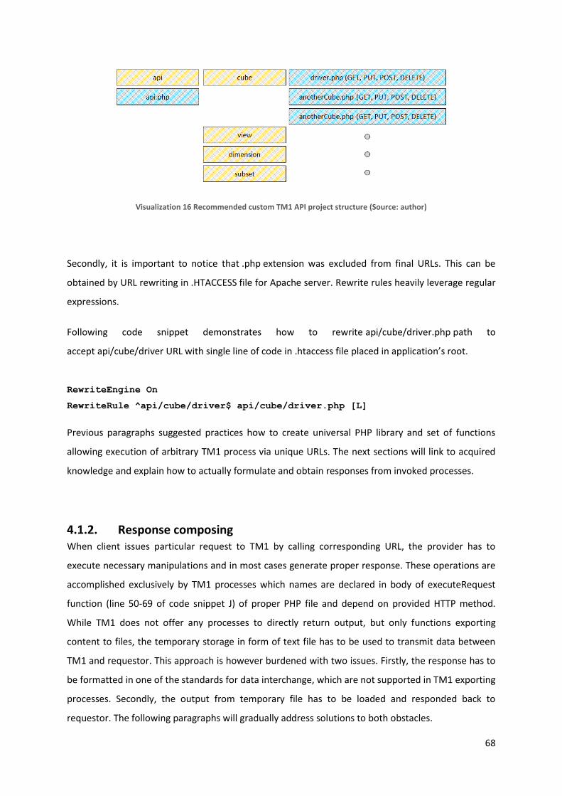
68
Visualization 16 Recommended custom TM1 API project structure (Source: author)
Secondly, it is important to notice that .php extension was excluded from final URLs. This can be
obtained by URL rewriting in .HTACCESS file for Apache server. Rewrite rules heavily leverage regular
expressions.
Following code snippet demonstrates how to rewrite api/cube/driver.php path to
accept api/cube/driver URL with single line of code in .htaccess file placed in application’s root.
RewriteEngine On
RewriteRule ^api/cube/driver$ api/cube/driver.php [L]
Previous paragraphs suggested practices how to create universal PHP library and set of functions
allowing execution of arbitrary TM1 process via unique URLs. The next sections will link to acquired
knowledge and explain how to actually formulate and obtain responses from invoked processes.
4.1.2. Response composing When client issues particular request to TM1 by calling corresponding URL, the provider has to
execute necessary manipulations and in most cases generate proper response. These operations are
accomplished exclusively by TM1 processes which names are declared in body of executeRequest
function (line 50-69 of code snippet J) of proper PHP file and depend on provided HTTP method.
While TM1 does not offer any processes to directly return output, but only functions exporting
content to files, the temporary storage in form of text file has to be used to transmit data between
TM1 and requestor. This approach is however burdened with two issues. Firstly, the response has to
be formatted in one of the standards for data interchange, which are not supported in TM1 exporting
processes. Secondly, the output from temporary file has to be loaded and responded back to
requestor. The following paragraphs will gradually address solutions to both obstacles.

69
4.1.2.1. JSON-like TM1 Text Output
Standard and most widely known system interoperability data formats are XML and JSON (MULLOY,
2012, p. 7). Despite XML longer history, JSON possesses set of benefits which led to its selection for
encoding data between PHP back-end and JavaScript front-end. JSON is easier to construct, read and
thanks to its prudent encoding also consumes less memory. In addition it is easier for PHP to encode
and for JavaScript frameworks to parse. These advantages can be perceived directly from definition
by json.org. JSON is a lightweight data-interchange format. It is easy for humans to read and write. It
is easy for machines to parse and generate (ECMA-262, 2011, p.201). As discussed in the previous
section, TM1 does not offer tools for encoding data directly to JSON and therefore some techniques
need to be applied in order to obtain required outputs. JSON is an array of objects which are
composed of pairs of names and values. Single cell from bi-dimensional cube
including Driver and Department dimensions such as ('FTE','ICT',123) can be encoded as follows:
JSON: {"Driver":"FTE","Department":"ICT","Value",123}
In the previous example "Driver":"Department" is the pair of name/value and the whole string
within {} is JSON object. When more objects are joined together and separated by comma, the array
of JSON objects is created.
When such output is requested from TM1 processes, some modifications, firstly introduced in my
blog post (FEDOROČKO, 2012a) have to be applied. Firstly, in order to block Turbo Integrator from
enveloping every variable into double quotes, the declareDatasourceASCIIQuoteCharacter local
variable in the Prolog tab has to be assigned empty value. Secondly, the TextOutput function needs
to be formatted as follows:
TextOutput('C:\...\...\file.txt','{"Driver":"'|driver|'"','"Department":"'|department|'"','"Value":'|value
|'}');
Applied formatting includes:
Single quotes enclose whole expression and separate text from variables.
Variables are enveloped with double quotes (except numerical values).
Variable and double quote have to be separated with single quote and concatenated with
pipe (|).
Labels are also enclosed with double quotes.
70
When applying previous recommendations to all TM1 processes, every request when invoked, will
output almost JSON formatted data into file with known location. The content from this file has to be
however subsequently loaded and responded back to the requestor. The function processing data
transition is introduced in the following paragraph.
4.1.2.2. Data loading
Because every request is linked to response, the universal API library processing requests has to be
extended with global function enabling response handling. The function is attached in Appendix C –
Code Snippet K and based on the received file location parameter loads (line 12), finishes formatting
(line 13 and 17) and returns data for echoing back to requestor. Function can be observed in action in
previous Code Snippet J on line 63, where it loads and echoes encoded content to browser in case of
successful exporting.
4.1.3. Request invocating So far, the back end infrastructure including API library, Apache URL rewrite rules and set of
functions handling specific requests and providing responses has been introduced. In order to close
the API cicle, it is necessary to extend this functionality with front end code invocating requests and
processing responses. Whereas the purpose of the alternative visualization is to keep the user
experience as smooth as possible, I decided to implement asynchronous communication with back
end server via AJAX techniques. AJAX is a group of interrelated web development techniques used on
the client-side to create asynchronous web applications. With Ajax, web applications can send data
to, and retrieve data from, a server asynchronously (in the background) without interfering with the
display and behavior of the existing page (GARRETT, 2005). For the purpose of making AJAX requests
simple and fast to implement, numerous frameworks have been developed. For the custom TM1 API
I decided to leverage jQuery library for its syntax thriftiness, rich pallet of functions and recent
expansion to majority of Web 2.0 applications. [SHARP, 2010, p. 12] The syntax for making
asynchronous request is defined as jQuery.ajax(url[, settings]), where settings is a set of more than
30 voluntary parameters. TM1 API will leverage type parameter for HTTP method definition, data for
posting parameter values to the server, dataType for definition of response encoding and success as
well as error for response processing. The URL parameter is mandatory and points to the unique
REST URL of object which is supposed to be requested. The example of GET request to Driver cube is
in code Snippet L – AJAX GET method while POST in snippet M – AJAX POST method of Appendix C.

71
The request settings of both functions are declared on lines 3 – 5. Remaining parameters focus on
response processing closely discussed in the fourth part of the API cycle.
4.1.4. Response processing The majority of asynchronous calls have a callback action varying from a simple notification about
success or fail of the operation to complex data sets of structured data. In jQuery $.Ajax function, the
callback is processed under success and error settings within the same function body as request was
originally invoked. It is obvious that different requests will have different implementations of
successful responses. In case of GET method, the incoming JSON encoded data are possible to be
looped with $.each functions while key and value parameters allow further manipulation within the
set and objects. Example can be found in Code Snippet L – AJAX GET method of Appendix C (line 6-
10). Post methods are designed to send data to the server and usually do not receive data structures
however just notifications. In this case no further processing is required and message can be at most
outputted to the screen as implemented in Code snippet M on lines 7 -9. On the other hand, the
occurred failures are at the back-end side marked with 500 – Internal Server Error header and
therefore fall through to error handler where their message is retrieved through XHR object and
printed to the screen (lines 10-12).
Antecedent chapter introduced techniques and practices used to implement own custom TM1 API.
This process required synchronization and integration of four different parts of communication into
the single unified circle. While the back-end provider leveraged heavily TM1 native executable
wrapped in PHP code in order to automatically execute commands, form responses and manage the
API project structure, the front-end web interface relied on existing JavaScript frameworks,
significantly reducing time and code required to implement fully asynchronous application. Despite,
some applied techniques have been well known and used for a long time, the concept as whole has
never been introduced in any researched community or publication. It is obvious that such API would
not be able to compete with fully-fledged native TM1 interface due to the fact of security threads
and development seriousness, however taking in consideration its current maturity and capabilities,
custom API seems to be valuable replacement for developers and applications seeking options for
manipulating with TM1 from outside the native environment. This argument will be proved in the
next chapter, where introduced API will be used to create alternative visualization interfaces for
onDemand allocator.
72
4.2. onDemand allocator API
Despite many improvements the onDemand allocator has brought in contrast to standard concept,
its restriction to multidimensional table-space did not allow to fully leverage the potential of its
design and capabilities. The reasoning introduced in the previous chapter leaned on poor visual
displaying, omission of the color and radius properties for highlighting significant features as well as
on faint positioning and screen space exploitation. Moreover, the control over drilling and analysis
process has been conducted via cell values switching and subsequent process execution. The
suggested cure for the lurking usability issues have been found in transferring allocator’s
presentation layer to web browser, where proper languages and advanced frameworks can be used
to remedy existing limitations. However, this transfer of the logic needs to be supported by
development of proper communication channel between existing allocator’s body and novel
unconventional interface.
Taking in consideration presented mission, current chapter focuses on leveraging knowledge,
practices and libraries developed in general introduction to custom TM1 API for the purpose of
enabling communication with onDemand allocator from web browser via its own interface. The
implementation will maintain heavily introduced concepts and structures, but extends the set of
REST URLs with ones supporting specific allocator functions. On the other side, the API will cooperate
with TM1 server hosting onDemand allocator as presented in previous chapters. It is important to
highlight that no modifications of model are required, however interface leverages set of processes
developed exclusively for the purpose of enabling API to work.
The analysis in onDemand model is conducted exclusively in Trace cube allowing observation of
allocation hierarchy and its graduate drilling by selecting required nodes and executing allocation
processes. In addition to Trace cube, the definition of target center being analyzed is set up in simple
two dimensional Selection cube. Every other cubes hosted on the server serves purely for back-end
processing and do not require any direct communication with analyst through the web browser,
hence no interface is needed for these cubes. On the other hand, the necessity of controlling the
Trace and Selection cubes, calls for implementation of two standalone back-end objects handling
their manipulations. Taking in consideration suggested practices for API project structure, the objects
have to be available under following URLs:
http://domain/api/cube/selection for Selection cube
http://domain/api/view/trace for Trace cube
73
The inner implementation of both objects will depend on type of method invoking the
communication and is further discussed in the following paragraphs.
4.2.1. Selection object Selection object is responsible for two types of actions. It has either return the list of available target
units or set the center which will be analyzed. The inner implementation is attached in the Code
Snippet N – Selection object of Appendix C. For the purpose of receiving possible cost centers for
analysis, the object has to be invoked with GET method ordering the TM1RunTI to call parameter-
free getSelection TM1 internal process encapsulating procedures for creating selection and its
subsequent exporting to defined location (line 54). The extract is coined by createSelection process,
filtering the target centers dimension to subset based on the attribute defining location of element
within the cascade. The subsequent exportSelection process then ensures proper encoding of items
into JSON format. In case of unexpected error, the object returns HTTP 500 status with proper TM1
error message attached (line 60).
On the other hand, in case of necessity to remotely set the selected cost center from web browser,
the Selection object has to be invoked via POST method, allowing additional parameter to be brought
over. The implementation firstly controls if the parameter has been set (line 69) and issues proper
notification when not. The parameter handed to TM1RunTI has to be properly formatted by
concatenating parameter name and value into single variable (line 76). Subsequently, the
postSelection process is invoked in TM1, inserting the parameter value into proper cell of Selection
cube through CellPutN TurboIntegrator function (line 77). Whereas the method does not return any
data, no loading from temporary storage file is needed and response can be replaced by default
notification about successful execution (line 89).
4.2.2. Trace object Two types of actions can also be identified regarding the Trace object. Firstly, the analyst has to be able
to remotely clear and restart allocation process while receiving the single root node representing selected
center. In addition, the possibility to tag particular node and initiate drilling from web browser needs to
be enabled. In this case, parameter storing unique identification of desired trace code is handed to TM1
prior to execution of general drill procedure. From the described portfolio of actions, it is obvious that
parameter free restart can be invoked via GET while impulse to allocate specific node will be assigned the
POST method. In contrast to Selection cube, both method implementations will return JSON formatted
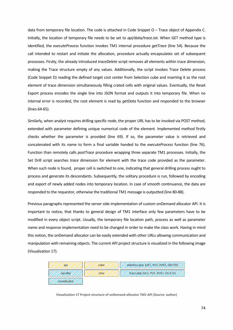
74
data from temporary file location. The code is attached in Code Snippet O – Trace object of Appendix C.
Initially, the location of temporary file needs to be set to api/data/trace.txt. When GET method type is
identified, the executeProcess function invokes TM1 internal procedure getTrace (line 54). Because the
call intended to restart and initiate the allocation, procedure actually encapsulates set of subsequent
processes. Firstly, the already introduced traceDelete script removes all elements within trace dimension,
making the Trace structure empty of any values. Additionally, the script invokes Trace Delete process
(Code Snippet D) reading the defined target cost center from Selection cube and inserting it as the root
element of trace dimension simultaneously filling crated cells with original values. Eventually, the Reset
Export process encodes the single line into JSON format and outputs it into temporary file. When no
internal error is recorded, the root element is read by getData function and responded to the browser
(lines 64-65).
Similarly, when analyst requires drilling specific node, the proper URL has to be invoked via POST method,
extended with parameter defining unique numerical code of the element. Implemented method firstly
checks whether the parameter is provided (line 69). If so, the parameter value is retrieved and
concatenated with its name to form a final variable handed to the executeProcess function (line 76).
Function than remotely calls postTrace procedure wrapping three separate TM1 processes. Initially, the
Set Drill script searches trace dimension for element with the trace code provided as the parameter.
When such node is found, proper cell is switched to one, indicating that general drilling process ought to
process and generate its descendants. Subsequently, the solitary procedure is run, followed by encoding
and export of newly added nodes into temporary location. In case of smooth continuance, the data are
responded to the requestor, otherwise the traditional TM1 message is outputted (line 80-88).
Previous paragraphs represented the server side implementation of custom onDemand allocator API. It is
important to notice, that thanks to general design of TM1 interface only few parameters have to be
modified in every object script. Usually, the temporary file location path, process as well as parameter
name and response implementation need to be changed in order to make the class work. Having in mind
this notion, the onDemand allocator can be easily extended with other URLs allowing communication and
manipulation with remaining objects. The current API project structure is visualized in the following image
(Visualization 17).
Visualization 17 Project structure of onDemand allocator TM1 API (Source: author)

75
Similar rule applies to the front-end invocation. Here, the body of jQuery $.Ajax function stays same
and various API calls differ in provided URL, parameters and callback processing. For the purpose of
better manipulation, every request will be enveloped in the standalone function ensuring easier
reuse and more transparent implementation during request synchronization. The request
synchronization is necessary in case of numerous consequent API calls. Because of the AJAX
asynchronous characteristics, subsequent code is executed immediately and do not wait for the
previous one to end. Whereas this could cause some TM1 processes to be executed in incorrect
order, the conjunctive invocations will be always synced this way. The function for requesting
allocation of particular node is attached in Code Snippet P – allocate of Appendix C. Because of the
bold similarities among all four API functions, remaining implementations will be omitted.
In order to test the functionality of implemented API and simultaneously provide useful and
empirical documentation for other developers, simple console allowing manual composition of
intended requests has been developed. The console can be reached at http://domain/api/console
location. Possible scenario of use is captured in the following screenshot (Visualization 18). While
the left pane enables manual composition of desired request comprised of type, object and its
method, the right pane is intended to append and show received response. The bottom row under
request panel dynamically constructs variables issued to jQuery Ajax function. Although, the
parameters are actually sent through data setting in function body, the bottom row represents their
alternative positioning at the end of the URL. However, because of the proper set up of rewrite rules,
the implemented object will be also capable of parsing such formatted request.
Visualization 18 Simple TM1 API test console (Source: author)
Previous paragraphs introduced practices necessary for solving presentation issues of novel
allocation approach. Set of implemented server-side objects in combination with techniques for their
76
comfortable invocation from web interface, made it possible to initiate design activities affiliated
with transformation of received data to various forms. Next paragraph closely introduces considered
concepts, their characteristics, determination to specific tasks and core implementation steps.
4.3. onDemand allocator alternative visualizations
The intention behind porting allocator’s presentation layer into web browser interface has not
emerged purely from attempts to mitigate usability obstacles linked to color distinguishing,
structuring and controlling, however contemplated to offer variety of visualization options for
specific types of tasks allocation analysts have to face. Taking in consideration defined goals, current
chapter focuses besides analysis of core components implementation also on identification of the
common use-case scenarios and their requirements. Acquired knowledge then allows designing
advanced visualizations comprised of the most suitable hierarchical structure, supplementary
information presentation and right control objects. The notion is supported with belief that only with
such level of perfection, reengineered novel approach to allocator can completely mitigate even the
last usability objection.
Based on the conducted research, interviews and experimentations, two most common analytical
tasks have been identified (COKINGS, 2006, p. 20; HORNGREN, 2006, p. 214). Firstly, the purpose of
the analysis can reside in the comparison of quantities on specific nodes in particular levels among
cost flows allocating to the single target element (HORNGREN, 2006, p. 214). In this case, analyst
drills fore-known traces in order to observe contrast in specific values. The comparison can either
focus on all or only single selected element within the allocation step. The possible scenario is
visualized in the following image (Visualization 19). Considering the hypothetical situation, where
third cascade refers to IT cost allocation, the analyst may be interested for instance how cost center
6 referring to internal project development contributed to the target center through various flows.
Possible differences in green cells may indicate how allocated costs and therefore provided services
have been utilized. Additionally, the entire cascade, comprised also of remaining centers can be
taken in account and compared altogether.

77
Visualization 19 Example of cost flow traces cmparison analysis (Source: author)
On the other hand, the analyst does not have to be aware in advance about the matter of fact which
needs to be analyzed, but attempts to find the cause of the occurred anomalies. The anomalies can
be represented by suspiciously high values or quantities significantly varying from ones recorded in
the corresponding time or version elements. In such case, the gradual ad-hoc analysis seems to be
appropriate. It comprises of subsequent selection and drilling of elements which appears to case the
observed anomaly with the highest probability. Situation can be visualized by following image
(Visualization 20). Considering the hypothetical abnormality at cost center 9, analyst subsequently
drills one level down to descendent nodes with intention to locate the source of the deviation. When
consecutively the cost center 7 appears as potential floater, it becomes the center of the analyst’s
interest and any other routes immediately loose their meaning for the current analysis. This ad-hoc
procedure is repeated until mere source of anomaly is identified.
Visualization 20 Example of drill-down ad-hoc analysis (Source: author)
In order to identify proper visualization techniques for presented approaches, numerous authors
discussing options for similar problem structures presentation have been researched (MANSMANN,
2007, p. 2; SCHUTZ, 2011, p. 8). The most appropriate concept can be found in Broadley’s (2002, p.
140) work suggesting tree and donut scheme as supplements for table space presentation of
hierarchical data. According Broadley, the tree layout is ideal for visualizing problem structure,
strength of relations and value of nodes. It is obvious that highlighted parameters are also the most
important features of allocation analysis. In addition, Mansmann (2007, p. 3) extends the concept

78
with suggestion of leveraging color pallet to distinguish quantitative information related to nodes.
Taking in consideration collected knowledge, the three dimensional design of possible views on
allocation structure has been developed (Visualization 21). Despite the model will be eventually
condensed into flat structure, it is necessary to introduced it in cubical space for better
comprehension of alignment with defined approaches. On top of the structure, in the first level lays
root node representing the target cost center selected for the analysis. In abeyance with onDemand
allocation principle, drilling one level down will reveal providers of quantity from previous allocation
step. These are placed under their ancestor connected with links to form the evolving cost flows.
Visualization 21 3D model of possible tree structure visualizations
It is obvious that observing the model from the front side and flattening it through z axis would show
particular drilled cost flows next to each other ordered in layers of allocation steps. Taking in
consideration assignments from first approach to allocation analysis, the view seems to be
appropriate for this kind of tasks. Analyst is firstly able to drill fore-known cost flows representing
subject of the interest and subsequently compare selected nodes within the single allocation step.
Whereas the view is designed to enable observation of contrasts in various nodes across single layer,
their quantitative values in each step will be represented by color hue from the attached palette.
Situation can be illustrated in the attached visualization no. 22, where initially six flows have been
drilled. Regarding its structure and utilization purpose, it will be further referred as comparison tree.
Within each layer, the node with the biggest value is highlighted with the brightest color, while

79
remaining centers are labeled with hues corresponding to their relative proportions. The
implementation of core actions and algorithms in comparison tree type of visualization will be closely
discussed in the next chapter.
Visualization 22 Front view on 3D model representing comparison tree structure (Source: author)
On the other hand, the presented structure would not be the most appropriate for the second type
of approach to allocation analysis. Whereas in this case analyst focuses less on comparison of
predefined traces, but rather on ad-hoc exploration of anomalies and suspicions flows, the view from
above the model through y axis seems to be more convenient (Visualization 22). Structure starts with
single root element in upper layer and by subsequent identification of desired nodes, analyst drills
down through the particular levels. However, as defined in the approach specification, by selecting
another component of suspicions cost flow, analyst simultaneously loose interest in remaining
unaffected nodes. Therefore, rather than consolidating particular layers and creating mass of nodes
during the drill, the view actually moves down the model and displays exclusively components from
current level. The only exception is drilled element which keeps in the visualization to create anchor
in case analyst would need to come back to higher layer. The concept was named Ad-hoc drill and is
visualized in the following Picture (Visualization 23). In the center of the visualization appears the
currently drilled node (layer X), which is connected to its gray ancestor (layer X+1) and
simultaneously to all of its descendants (layer X-1). The distance from the descendant to its parent in
the center of the visualization determines allocation level. In addition, similar color rule applies to all
nodes within the single step, distinguishing the differences in their quantitative values. The
implementation steps of the ad-hoc drill visualization technique will be discussed in more detail in
the following sections.

80
Visualization 23 View from above on 3D model representing drill-down ad-hoc structure (Source: author)
Both approaches heavily leverage basic graphic elements such as lines, circles and squares. However,
there does not exist any direct way how to draw them simply using only core JavaScript libraries.
Obviously, specific technologies such as Flash or Silverlight can be used, however I preferred not to
make the final application dependant on their presence in client’s workstation and simultaneously
mix in another languages which would require further transferring of already received data through
jQuery. The solution can be found in leveraging Raphael JavaScript library developed to simplify
usage of vector graphic in web browsers. The library is small in size, easy to use, supports SVG W3C
recommendations and works in all major browsers (BARANOVSKIY, 2012). Additionally it works
smoothly with already implemented jQuery, what significantly simplifies handing of received data
and manipulation with generated objects. The list of employed functions is recorded in the following
table (Table 12).
Table 12 List of employed Raphael functions (Source: author)
Function Affiliated action
Paper.circle(x,y,r) Draws circle with radius r in position defined by x and y coordinates.
Paper.path([pathString]) Draws a path according provided path string including start and end point coordinates.
Paper.rect(x,y,w,h, [r]) Draws a rectangle with provided width and height and voluntary rounded corners.
Moreover, presented objects can be formatted by providing additional parameters or animated by
specifying predefined actions and events. Finally, every object can be extended with numerous self-
defined variables temporarily keeping necessary information. This is a crucial condition while nodes

81
need to be data rich and intelligent in order to properly format and position within the structure and
seemly react to analyst’s actions. The attributes and data for every element are encoded and
received in incoming JSON response. Exemplary record can be represented as encoded in the
following code snippet:
{"trace":"PRIMARY.9:CC18.2:CC03","node":"CC03","nodeID":"19","level":"2","p
arentNodeID":"5","solve":"0","type":"0","value":"71.42857142857143"}
Following table (Table 12) clarifies meaning and usage of every item within the object.
Table 13 Explanation of particular values received in incoming JSON object (Source: author)
Item Meaning Usage
Trace Unique trace code of the node. Used for administrative and control purposes.
Node Name of the node (cost center). Displays cost center name.
nodeID Unique numerical identificator of
the trace code.
Used for unique identification of the node and parameter transferred
in drill request (POST method in Trace view API call) to allocator.
Level Level or allocation steps where
the node has been processed.
Used to correctly position the object within a level layers representing
node.
parentNodeID Unique numerical identificator of
the parent trace code.
Identifies parent node when drawing cost flow connectors.
Solve Boolean attribute identifying
possibility of further drilling.
Determines wheatear drill event ought to be appended to the node.
Type Boolean attribute distinguishing
primary and secondary values.
Determines how the node is supposed to be displayed.
value Actual quantitative value of the
node.
Displays the quantitative value of the node and determines what
color from the pallet has to be applied.
Having the most common approaches to allocation analysis defined as well as their means of
structuring and used techniques, the following paragraphs draw the core concepts, algorithms and
actions use in both visualizations.
4.3.1. Comparison tree visualization Comparison tree visualization is captured in the following screenshots (Visualizations no. 24 and 25).
Despite its proportion into three standalone widgets, only the middle area varies for presented
approaches. Left pane is dedicated to application operation and presentation of detailed
information. On the other hand right vertical pallet serves as ruler for gross estimation and
comparison of node values. Whereas side panels are mutual for both visualizations, they are
developed and included from the external sources. Following section firstly explains actions hidden
behind general operation console in the left pane before moving to solitary presentation window.

82
Visualization 24 Exemplary analysis in compariosn tree structure (Source: author)
Visualization 25 Exemplary analysis in compariosn tree structure (Source: author)
The select center list box in the operation pane is being populated leveraging API call returning
values from Selection cube. After the definition of desired target center, the analysis can be invoked
through allocation button, executing sequence of graduate functions, comprised of setting up the
root node, restarting the Tracing cube and drilling down the first level. Appropriate code is captured
in the code snippet P – of the Appendix D. Initially listener linked to the button reads the name of the
target center in list box, passes it to the postSelection function (line 6) and eventually temporarily

83
disables the button. Inner implementation of postSelection function ensures writing received cost
center name into the appropriate TM1 cube (line 19). Because of the asynchronous fashion of AJAX
functions, the following application restart needs to be invoked even from its callback section (line
27). In case of the successful restart, the received root element is placed into the presentation
widget (line 53), enriched with necessary attributes and immediately drilled via postTrace function
with default parameter (line 60). Returned set of elements represents first descendants of root node
further processed, positioned and formatted based on the specific type of visualization. The inner
implementation for comparison tree visualization is captured in the code snippet Q of Appendix D. In
case of successful response admission, the appropriate random position based on the node level
information is generated (lines 4-7). Having the placement parameters defined, they are handed to
createNode function, establishing the new instance of circle object, filling it with necessary
parameter, appending to screen and returning into variable.
Furthermore, visualized cost centers need to support core mouse event actions, in order to allow
analyst comfortable manipulation and perception of additional information. For the purpose of
manipulation with particular nodes, the onClick event has been implemented. However, by clicking
on selected element, two different actions may possibly be intended to invoke, comprised of drilling
or removing current object. In order to distinguish required action, the operation console is extended
with remove check-box. When the remove parameter is checked, the node is cleaned up from the
screen (line 16). On the other hand, when the intention of the analyst is not to remove existing
nodes, clicking on the element can either drill and append new descendants (line 25), or in case of
already opened nodes change the visibility of all child nodes (27). Functions for invoking drilling and
changing visibility of child nodes are captured in code snippets R and S of Appendix D.
Additionally, mouse event is supposed to foster hovering gestures. In this case entered node not
only highlights parent object, all descendants and their connections however also provides additional
information in left side box, comprise of cost centers quantitative value, its name, level and parent
node. Moreover, the hover gesture similarly needs to distinguish among two types of actions. In
order to keep the presented information consistent, the lines connecting nodes and representing
relations are showed only temporary during hovering over selected element. However, for
comparison purposes some connections are required to be displayed permanently. Therefore, the
operation console has been additionally extended with connect checkbox, identifying how
application ought to handle relations when mouse leaves the node area. Both hover and unhover
actions are implemented in eponymous functions captured in code snippets T – hovering of Appendix
D. Immediately after cursor enters node area, appropriated parameters are extracted from
temporary variables and displayed in the left information panel, allowing smoother orientation

84
among nodes and their easier analysis (lines 11-14). Additionally, relevant nodes including parent and
descendant objects are connected according node’s current state and connect checkbox, followed by
visual highlighting of both groups. In opposite, mouse leaving object firstly invokes clearing of node’s
detail from left information panel and secondly, based on the analyst desire to observe allocation
relations, decides about maintaining or hiding particular connections (line 43-54).
At the end of the received data processing and after all mouse event actions have been defined,
function executes script looping through all levels and recoloring nodes based on their quantitative
values in comparison to remaining elements within single level. The recolorAllLevel script is recorded
in code snippet U of appendix D. The script heavily leverages HSL color model to transfer percentual
values into appropriate colors from the pallet (line 16). Moreover, with intention to avoid circles
overlaying, the bounceCircle function has been implemented, ensuring that in case of nodes collision,
they are appropriately reposition to new location, keeping the visual experience of Comparison tree
unaffected. The bounceCricle function is captured in the code snippet V of appendix X. The collision
can be easily identify thanks to Raphael’s core functionality allowing comparison of element’s
positions (line 15). In case of the positive diagnosis, the elastic mode is applied to animate
reallocation of affected nodes, while the callback recursively executes function again, to avoid nodes
being placed into another colliding position.
Previous sections introduced in detail implementation of Comparison tree visualization interface.
Next paragraph in contrast suggests how to transform existing functions into Ad-hoc drill layout.
Although totally different approach and view on the data will be used, majority of code will be kept
unaffected and only significant modification will be done to data processing and positioning. This
simultaneously proves how can be custom TM1 API and introduced frameworks leveraged in order to
build own, agile, expeditious and advanced visualizations.
4.3.2. Ad-hoc Drill visualization Ad-hoc drill visualization captured in the following screenshots (Visualization 26 and 27) is composed
from exactly same widgets as Comparison tree layout introduced in the previous section. Also the
logic and inner implementation of operation console has not change and stays the same as one
explained in code snippet P of Appendix D. It is important to notice, however, that both remove and
connect checkboxes have been cut off, since ad-hoc concept does not required various handling of
single mouse event.
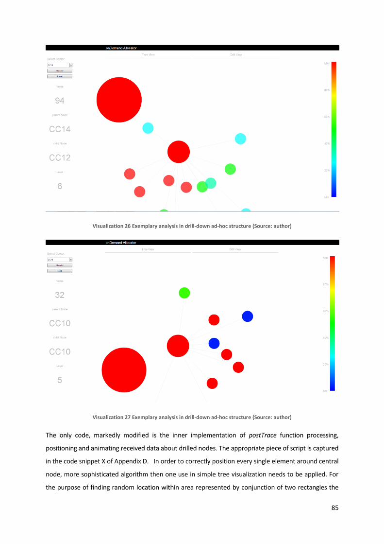
85
Visualization 26 Exemplary analysis in drill-down ad-hoc structure (Source: author)
Visualization 27 Exemplary analysis in drill-down ad-hoc structure (Source: author)
The only code, markedly modified is the inner implementation of postTrace function processing,
positioning and animating received data about drilled nodes. The appropriate piece of script is captured
in the code snippet X of Appendix D. In order to correctly position every single element around central
node, more sophisticated algorithm then one use in simple tree visualization needs to be applied. For
the purpose of finding random location within area represented by conjunction of two rectangles the
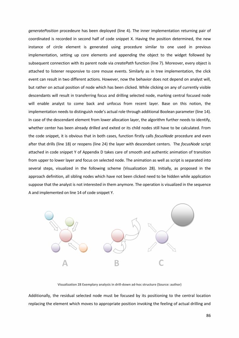
86
generatePosition procedeure has been deployed (line 4). The inner implementation returning pair of
coordinated is recorded in second half of code snippet X. Having the position determined, the new
instance of circle element is generated using procedure similar to one used in previous
implementation, setting up core elements and appending the object to the widget followed by
subsequent connection with its parent node via createPath function (line 7). Moreover, every object is
attached to listener responsive to core mouse events. Similarly as in tree implementation, the click
event can result in two different actions. However, now the behavior does not depend on analyst will,
but rather on actual position of node which has been clicked. While clicking on any of currently visible
descendants will result in transferring focus and drilling selected node, marking central focused node
will enable analyst to come back and unfocus from recent layer. Base on this notion, the
implementation needs to distinguish node’s actual role through additional Boolean parameter (line 14).
In case of the descendant element from lower allocation layer, the algorithm further needs to identify,
whether center has been already drilled and exited or its child nodes still have to be calculated. From
the code snippet, it is obvious that in both cases, function firstly calls focusNode procedure and even
after that drills (line 18) or reopens (line 24) the layer with descendant centers. The focusNode script
attached in code snippet Y of Appendix D takes care of smooth and authentic animation of transition
from upper to lower layer and focus on selected node. The animation as well as script is separated into
several steps, visualized in the following scheme (Visualization 28). Initially, as proposed in the
approach definition, all sibling nodes which have not been clicked need to be hidden while application
suppose that the analyst is not interested in them anymore. The operation is visualized in the sequence
A and implemented on line 14 of code snippet Y.
Visualization 28 Exemplary analysis in drill-down ad-hoc structure (Source: author)
Additionally, the residual selected node must be focused by its positioning to the central location
replacing the element which moves to appropriate position invoking the feeling of actual drilling and

87
keeping the anchor for possible way back (sequence B, lines 18 & 21). Eventually, the focused node
looks similarly to one visualized on the C sequence, ready to be enriched with its descendants.
Considering the situation when analyst requires coming up from drilled flow and obtaining the
exactly same view as one presented before the actual drill, the reverse actions bounded to the
focused central node needs to be executed. The transformation is ensured by sequence of three
subsequent functions. Firstly, all descendants of node currently being unfocused are hidden by
animation in opposite fashion as ones being appended to the widget (line 28). In addition, currently
offset center needs to be transferred back into middle location while the focused elements is
suppose to be position back, at the exact same position from which was previously centered (line
29). Eventually, siblings previously hidden because of the lack of analyst interest are summoned back
to their original position and linked with their parent node (line 30).
At the end of every data processing, all currently visible nodes need to be recolored based on their
quantitative values compared to remaining elements from the same allocation step.
Previous section introduced uncommon visualization techniques applied to onDemand cost
allocation. It simultaneously closed the second half of the thesis specialized on custom TM1 API
development and its application to implementation of advanced visualization. During pages
dedicated to these topics, I introduced novel approach to communication with TM1 from outside the
native environment and proposed simple general libraries, concepts and structures required to
develop own interface on top of modified TM1 server. Recommendations emerged from knowledge
collected during extended period of time from industry best practices and standards, while the
feasibility of proposed concept was allowed to be empirically tested on basic supplementary console
developed exclusively for custom TM1 API. Furthermore, I elaborated the theoretical concept into
four tangible functions allowing communication and remote operation of previously developed
onDemand allocation server. The success of the research and design has been eventually confirmed
during implementation of two advanced visualization web applications heavily employing mentioned
API requests.
88
5. Conclusion
With intention to put the obsolescent cost allocation model back to the game and conform it to
current requirements and novel standards, multiple subsequent analyses, design tasks and
implementation experiments needed to be conducted during the taken off project of its innovation.
Reaching the end of the thesis representing verbal substantiation of performed project, it is possible
to assuredly declare that it has successfully solved all goals affiliated with removing existing hurdles
and proposing novel approaches to communication and presentation of allocation data.
Initially I analyzed original methodology proposed in my bachelor thesis and already implemented
solutions to identify core weaknesses emerging into standard approach during time. Among issues
negatively influencing awareness were classified arguments affiliated with application performance
and possibility to audit generated data flows. Moreover, the poor usability of generic table structures
and final presentation capabilities were included into composed list of properties restricting the
movement with the technology trends.
Collected issues have been further transformed into four standalone hypothesis submitted to the
continuous verification of ideas outgoing from the experimentations and brainstorming sessions. The
primary focus of these reengineering premises laid in design of the novel allocation concept
debugging as much as possible weaknesses. Finally, the promising solution was found in simple
model reversion, providing the most important information first and then allowing voluntarily
exploration of detailed data based on the analyst’s interest. Eventually the thesis verified viability of
designed model by putting it into practice and implementing general onDemand allocation model in
IBM Cognos TM1.
In order to measure how successfully novel approach removes particular issues and benefits it
possibly brings to enterprises interested in its implementation, I researched and suggested complex
model for benchmarking two separate OLAP applications. The model consists of four dimensions and
touches every aspect of possible influence, selected model can have on implementing organization.
Proposed perspectives includes except performance and usability metrics also development
complexity and rarely used consolidating financial benefits, both models can generate. At the end of
the conducted experiments, measurements and interviews, positive results for onDemand model
have been recorded in all four dimensions what eventually confirmed the possibility to diminish all
issues and qualities of suggested reengineered concept.

89
In the second half, thesis focused on design and development of general custom TM1 API, enabling
the communication and data transfer among different applications with intention to finally build
standalone presentation layer allowing advanced visualizations, removing even the last limitations
native TM1 cube space can have. Firstly the complex bi-directional communication circle between
web browser front-end and TM1 server was presented. Additionally I suggested universal project
structure and developed core API library, allowing rapid production of specific classes handling
requests to particular TM1 objects. The viability of implemented interface was firstly proved by
simple web console attached to the API project for testing purposes. Moreover proposed practices
have been applied to existing onDemand model and leveraged during development of two custom
interfaces conforming to the most common analytical tasks.
I believe that especially these applications, their agility, speed and usability are the most tangible
proof of successful fulfillment of defined goals and reengineering attempts. Moreover, I hope that
thesis can serve as basis for igniting the unconventional thinking about approaching similar tasks and
designing usable interfaces. In addition, I am persuaded that the proposed benchmarking model will
mean the significant contribution to all developers and consultants willing to benchmark different
implementation versions of their OLAP models. Despite I am sure, that porting existing planning and
what-if applications to new web interfaces via proposed API would be in current state in most cases
time consuming, risky and almost impossible, I believe that it can be already leveraged for some
smaller tasks. Possible utilization can be found in replacing fully-fledged planning clients with small
custom build TM1 API widgets, integrated into portals and allowing direct uploading of data.
However, the thesis is so broad, multi-topic and information exhausting that it is clear that every
reader will find insight interested and useful for her needs.
On the other hand, there is still much to do. In the near future I plan to extend the core onDemand
model with additional dimensions allowing comparison across various versions or demanded context.
This will however simultaneously place requirements on modifying the core API libraries and
adjusting visualization interfaces with techniques enabling comparison of multiple values.
Furthermore, it is necessary to elaborate advanced security practices for transferring and temporary
storing data in unsecured files. The promising option seems to be forwarding responses via Cognos BI
reports in XML structure and consuming them with its complex SDK. While various pros and cons
emerge on both sides, it is obvious that deeper research and experimentation would be required.
Eventually, I am aware that the proposed benchmarking model still needs enrichment with new
perspectives, amplification of metrics and improvement of equation and practices used for their
evaluation.
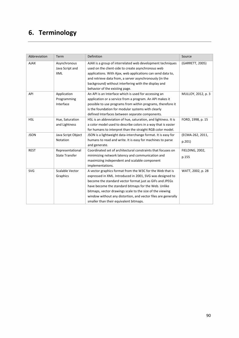
90
6. Terminology
Abbreviation Term Definition Source
AJAX Asynchronous
Java Script and
XML
AJAX is a group of interrelated web development techniques
used on the client-side to create asynchronous web
applications. With Ajax, web applications can send data to,
and retrieve data from, a server asynchronously (in the
background) without interfering with the display and
behavior of the existing page.
(GARRETT, 2005)
API Application
Programming
Interface
An API is an Interface which is used for accessing an
application or a service from a program. An API makes it
possible to use programs from within programs, therefore it
is the foundation for modular systems with clearly
defined Interfaces between separate components.
MULLOY, 2012, p. 3
HSL Hue, Saturation
and Lightness
HSL is an abbreviation of hue, saturation, and lightness. It is
a color model used to describe colors in a way that is easier
for humans to interpret than the straight RGB color model.
FORD, 1998, p. 15
JSON Java Script Object
Notation
JSON is a lightweight data-interchange format. It is easy for
humans to read and write. It is easy for machines to parse
and generate.
(ECMA-262, 2011,
p.201)
REST Representational
State Transfer
Coordinated set of architectural constraints that focuses on
minimizing network latency and communication and
maximizing independent and scalable component
implementations.
FIELDING, 2002,
p.155
SVG Scalable Vector
Graphics
A vector graphics format from the W3C for the Web that is
expressed in XML. Introduced in 2001, SVG was designed to
become the standard vector format just as GIFs and JPEGs
have become the standard bitmaps for the Web. Unlike
bitmaps, vector drawings scale to the size of the viewing
window without any distortion, and vector files are generally
smaller than their equivalent bitmaps.
WATT, 2002, p. 28
91
7. Resources
ACORN SYSTEMS. Enterprise Performance Suite: Software for High Performing Organizations. Acorn
Systems [online]. 2012 [2012-08-11]. Available at:
<http://www.acornsys.com/Portals/76901/docs/pb.Enterprise-performance-suite.pdf>.
ACHOR, Tom. Using Online Analytical Processing Tools. Pennsylvania: CPA Journal, 2002, volume 72,
issue 3. ISSN 0746-1062.
ALARCON, Rosa; PAUTASSO, Ceasare; WILDE, Eric. Proceedings of the Second International
Workshop on RESTful Design, WS-REST 2011, Hyderabad, India, 2011. ACM 2011, ISBN 978-1-4503-
0623-2. Available at: <http://ws-rest.org/2011/wsrest2011-proceedings.pdf>.
BARANOVSKIY, Dmitry. Raphäel: JavaScript Library. Raphäel [online]. 2012 [2012-10-06]. Available at:
<http://raphaeljs.com/>.
BARNES, Dan. Technology: Spreadsheet Risk: Spreadsheets Are Vital Tools For Traders And Banks'
Back-office Staff But Their Flexibility Can Weaken Governance. Dan Barnes Looks At The Problems
And The Potential Solutions. The Banker. London, United Kingdom: The Financial Times Limited, 2006.
ISSN 00055395.
BORDLEY, Robert. Representing trees using Microsoft doughnut charts. The American Statistician.
Alexandria, Virginia: American Statistical Association, 2002, volume 56, issue 2. ISSN 1537-2731.
BOTHE, Ondřej. IBM. Performance Management: What-if?. Prague, 2007. IBM Internal Document -
Presentation.
BOTHE, Ondřej; FEDOROČKO, Peter. IBM. Interview with undisclosed business partner. 2011. IBM
Internal Document - Interview.
BOTHE, Ondřej; FEDOROČKO, Peter. IBM. Interview with undisclosed customer. 2010. IBM Internal
Document - Interview.
CARPEDATUM CONSULTING. Built-in TM1 API Functions. CarpeDatum Inc. [online]. 2012 [2012-10-
14]. Available at: <http://www.carpedatuminc.com/Products/ESTM1API.aspx>.
COKINGS, Gary. INSTITUTE OF MANAGEMENT ACCOUNTING. Implementing Activity-Based Costing.
New Jersey, 2006. Available at:
<http://www.imanet.org/PDFs/Public/Research/SMA/Implementing%20Activity%20Based%20Costin
g.pdf>.
COSTEA, Adrian. On Measuring Software Complexity. Journal of Applied Quantitative Methods.
Romania: Association for Development through Science and Education, 2007, volume 2, issue 1. ISSN
1842–4562. Available at: <http://jaqm.ro/issues/volume-2,issue-1/pdfs/costea.pdf>.
CUBE BILLING. Cost Allocation Solutions. Cubebilling [online]. 2012 [2012-8-08]. Available at:
<http://www.cubebilling.com/Solutions.aspx>.

92
DRURY, Colin. Management and cost accounting. 7th ed. London: Thomson, 2008. ISBN 18-448-0028-
8.
ECMA-262. ECMAScript Language Specification. Geneva: ECMA International, 2011. Available at:
<http://www.ecma-international.org/publications/files/ECMA-ST/Ecma-262.pdf>.
FEDOROČKO, Peter. JSON-like TM1 Text Output. Analytics Humanly [online]. Prague, 2012b [cit. 2012-
10-14]. Available at: <http://www.analyticshumanly.com/2012/10/json-like-tm1-text-output.html>.
FEDOROČKO, Peter. TM1RunTI Guide. Analytics Humanly [online]. Prague, 2012a [2012-10-14].
Available at: <http://www.analyticshumanly.com/2012/10/tm1runti-guide.html>.
FEDOROČKO, Peter. Optimization of costs and product profitability using what-if analysis in reciprocal
cost allocation model. Prague, 2010a. Bachelor Thesis. University of Economics in Prague. Supervisor
Jan Pour.
FEDOROČKO, Peter; BOTHE Ondřej. IBM. Cost Allocation Methodology. Prague, 2010b. IBM Internal
Document.
FEST, Glen. The Future of Spreadsheets in BI? Excel-Lent. Bank Technology News. New York:
SourceMedia, 2007, volume 20, issue 6. ISSN 10603506.
FIBÍROVÁ, Jana et al. Nákladové a manažerské účetnictví. 1th. Prague: ASPI, a.s., 2007, 423 p. ISBN
978-80-7357-299-0.
FIELDING, Roy a Richard TAYLOR. Principled Design of the Modern Web Architecture. ACM
Transactions on Internet Technology. New York: Association for Computing Machinery, 2002, volume
2, issue 2. ISSN 1533-5399.
FITZPATRICK, Ronan. Strategies for Evaluating Software Usability. Dublin: Methods, 1998, volume
353, issue 1. ISSN 1046-2023. Available at:
<http://arrow.dit.ie/cgi/viewcontent.cgi?article=1000&context=scschcomart>.
FORD, Adrian; ROBERTS A. Colour Space Conversions. United Kingdom, 1998. Available at:
<http://www.poynton.com/PDFs/coloureq.pdf>.
GARRETT, James. Ajax: A New Approach to Web Applications. Adaptive Path [online]. 2005 [cit. 2012-
11-09]. Available at: <http://www.adaptivepath.com/ideas/ajax-new-approach-web-applications>.
GARTNER. Magic Quadrant for Business Intelligence Platforms. Stamford, Connecticut, 2011.
GARTNER. Magic Quadrant for Corporate Performance Management Suits. Stamford, Connecticut,
2010.
GOIL, Sanjay. High Performance OLAP and Data Mining on Parallel Computers: Data Mining and
Knowledge Discovery. Hingham, MA: Kluwer Academic Publishers, 1997, volume 1, issue 4. ISSN
1384-5810. Available at:
<http://reference.kfupm.edu.sa/content/h/i/high_performance_olap_and_data_mining_on_67286.p
df>.

93
GYANWALI, Pawan. .Net TM1 API. SOURCEFORGE. SourceForge [online]. 2007 [2012-10-14]. Available
at: <http://sourceforge.net/projects/tm1-api/files/>.
HANSEN, Don; MOWEN Maryanne. Cost Management: Accounting and Control. 4th Ed. Thomson:
South-Western, 2003, 1029 p. ISBN 03-240-6973-1.
HORNGREN, Ch; SUNDEM, G. Management Accounting: Fifth Canadian Edition. Canada: Pearson
Education, 2006. ISBN 978-0131922686. Available at:
<http://www.pearsoned.ca/highered/divisions/virtual_tours/horngren/man_acc/Ch05ManAcc.pdf>.
HSIAO, Tim; PETCHULAT. Data visualization on web-based OLAP: Proceedings of the ACM 14th
international workshop on Data Warehousing and OLAP. New York: Association for Computing
Machinery, 2011, pages. 75-82. ISBN 978-1-4503-0963-9.
IBM. Using TM1RunTI, IBM Infocenter [online]. 2011b [2012-10-14]. Available at:
<http://pic.dhe.ibm.com/infocenter/cx/v10r1m0/index.jsp?topic=%2Fcom.ibm.swg.ba.cognos.tm1_t
urb.10.1.0.doc%2Fc_tm1_op_usingtm1runti.html>.
IBM. TM1 API Guide. United States, 2011a. Available at:
<http://www.olapline.de/fileadmin/user_upload/00003_Doc/01_Pdf/TM1/tm1_api.pdf>.
ISO/IEC 25000. Software engineering — Software product Quality Requirements and Evaluation
(SQuaRE) — Guide to SQuaRE. Geneva: ISO, 2005.
KAPLAN, Robert; COOPER Robin. Cost & Effect: Using Integrated Cost Systems to Drive Profitability
and Performance. Boston: Harvard Business Press, 1997. ISBN 0875847889.
KATHAGE, Frank. Cost Allocation. Zeb Control [online]. 2012 [2012-8-11]. Available at:
<http://www.zebcontrol.com/banking/products/zebcontrol-financial/cost-allocation.html>.
KEARNEY, Joseph et al. Software Complexity Measurement. Communications of the ACM. New York:
Association for Computing Machinery, 1986, volume 29, issue 11. ISSN 0001-0782. Available at:
<http://sunnyday.mit.edu/16.355/kearney.pdf>.
KELLER, Craig. Simpler than ABC: New Ideas for Using Microsoft Excel for Allocationg Costs.
Management Accounting Quarterly. Montvale, New Jersey: Institute of Management Accountants,
2005, volume 6, issue 4. ISSN 1528-5359.
LEESE, Wallace et al. Using Excel's Matrix Operations to Facilitate Reciprocal Cost Allocation.
American Journal of Business Education. Littleton, Colorado: Clute Institute for Academic Research,
2009, volume 2, issue 9. ISSN 1942-2504.
LENGSTORF, Jason. Pro PHP and jQuery: Add quick, smooth, and easy interactivity to your PHP sites
with jQuery [online]. United States of America: Apress, 2010 [2012-10-10]. ISBN 978-1-4302-2848-6.
MANSMANN, Svetlana; SCHOLL Marc; KEIM Daniel; MANSMANN Florian. Exploring OLAP Aggregates
with Hierarchical Visualization Techniques: IEEE Symposium of Information Visualization. Konstanz,
Germany, 2006. Available at: <http://kops.ub.uni-
konstanz.de/bitstream/handle/urn:nbn:de:bsz:352-opus-69136/MaScKe06.pdf?sequence=1>.
94
MARTIN, Wolfgang, NUßDORFER, Richard. CPM – Corporate Performance Management: White
Paper: Analytical Services in a SOA. 4th. Munich, Germany, 2008. Available at:
<http://www.panoratio.com/fileadmin/files/download/SOA_Forum_CPM-
Corporate_Performance_Mgt._V2_english.pdf>.
MEKTEROVIĆ, Igor; BARANOVIĆ Mirta. Developing a General Purpose OLAP Client Prototype Using
XML for Analysis. Zagreb, Croatia, 2005. Available at: <http://bib.irb.hr/datoteka/202850.BIS20.pdf>.
MISRA, Sanjay et al. Weighted Class Complexity: A Measure of Complexity for Object Oriented System.
Journal of Information Science and Engineering. Taiwan: Institute of Information Science, Academia
Sinica, 2008, volume 24, issue 1. ISSN 1016-2364. Available at:
<http://www.iis.sinica.edu.tw/page/jise/2008/200811_05.pdf>.
MULLOY, Brian. APIGEE. Web API Design: Crafting Interfaces that Developers Love. Palo Alto,
California, 2012.
MUNDY, Joy. Relating to OLAP. Intelligent Enterprise. San Mateo: United Business Media LLC, 2002,
volume 5, issue 16. ISSN 15243621.
NOORVEE, Lembi. Evaluation of the effectivness of internal control over financial reporting. Tartu,
Estonia, 2006. Available at:
<http://dspace.utlib.ee/dspace/bitstream/handle/10062/1315/noorveelembi.pdf> Master Thesis.
University of Tartu. Supervisor Toomas Haldma.
OKTAY, Melek et al. Architectural, Technological and Performance Issues in Enterprise Applications.
Paris: World Academy of Science, Engineering and Technology, 2007, volume 1, issue 3. ISSN 2010-
3778. Available at: <http://www.waset.org/journals/waset/v3/v3-40.pdf>.
OLAP COUNCIL. APB-1 OLAP Benchmark: Release II. 1998. Available at:
<http://www.olapcouncil.org/research/APB1R2_spec.pdf>.
ORACLE. PeopleSoft Enterprise Project Costing. Redwood Shores, California, 2009. Available at:
<http://www.oracle.com/us/products/applications/peoplesoft-enterprise/service-
automation/057290.pdf>.
POPESKO, Boris. Moderní metódy řízení nákladu: Jak dosáhnout efektivního vynakládání nákladu a
jejich snížení. 1th. Prague: Grada Publishing, a.s., 2009, 240 p. ISBN 978-80-247-2974-9.
RASIEL, Ethan. The McKinsey Way: Using the Techniques of the World's Top Strategic Consultants to
Help You and Your Business. United States of America: McGraw-Hill, 1999. ISBN 0-07-136883-3.
SAGE PFW. Sage PFW ERP: Advanced Allocations. Sage PFW [online]. Irvine, California, 2009 [2012-
10-14]. Available at: <http://www.sagepfw.com/library/PFW_FS_AdvancedAllocations.pdf>.
SALMON, Janet. SAP. Controlling with SAP — Practical Guide. Bonn: Galileo Press, 2011. ISBN 978-1-
59229-392-6.
SEFFAH, Ahmed et al. Usability measurement and metrics: A consolidated model. Montreu, Quebec:
Springer Science+Business Media, 2006, issue 14. ISSN 1573-1367. Available at:
<http://psych.concordia.ca/fac/kline/library/sdkh06.pdf>.

95
SHARP, Jonathan. JQuery Cookbook: Solutions and Examples for jQuery Developers. 2nd. United
States of America: O'Reilly, 2010. ISBN 978-0-596-15977-1.
SCHULZ, Hans-Jorg. Point-Based Visualization for Large Hierarchies: The IEEE Transactions on
Visualization and Computer Graphics. Washington, DC: IEEE Computer Society, 2011, volume 17,
issue 5. ISSN 1077-2626. Available at: <http://www.informatik.uni-
rostock.de/~hs162/pdf/pbinvited.pdf>.
SLEIGH, Cynthia; JOHARI, Iman. IBM DEVELOPER WORKS. Get started with the IBM Cognos Mashup
Service: Fast application development for Cognos BI report content. Canada, 2010. Available at:
<http://www.ibm.com/developerworks/data/library/techarticle/dm-1001cognosmashup/dm-
1001cognosmashup-pdf.pdf>.
SPOFFORD, George. Access to intelligence : The New OLAP API's. Intelligent Enterprise. San Francisco:
Inderscience Publishers, 2006, volume 5, issue 15. ISSN 1745-3240.
TAGETIK. Cost Allocation & Profitability Analysis. Tagetik [online]. 2012 [2012-8-11]. Available at:
<http://www.tagetik.com/software/pm/cost-allocation-profit>.
U.S. DEPARTMENT OF EDUCATION. Cost Allocation Guide for State and Local Governments.
Washington, DC: Office of the Chief Financial Officer, 2009. Available at:
<http://www.ed.gov/about/offices/list/ocfo/fipao/icgindex.html>.
VOLLMERHAUSE, Allan; ERGON. Cost Allocation Method. 1th. Jackson, Mississippi, 2009. Available at:
<http://www.ergon.com.au/__data/assets/pdf_file/0013/6313/Cost-Allocation-Method.pdf>.
WATT, Andrew. Designing SVG web graphics. 1th edition. Indianapolis, Ind.: New Riders, 2002, 544 p.
ISBN 07-357-1166-6.
ZANAJ, Elma et al. Multidimensional analysis in intelligence business systems. International Journal of
Computer Science and Information Security. Pittsburgh: L J S Publishing, 2012, volume 10, issue 5.
ISSN 1038151862.

96
8. List of visualizations
Visualization 1 Cost Allocation model evaluation framework (FEDOROČKO, 2010, p. 26) ................... 19
Visualization 2 Cascade allocation matrix example (Source: author) ................................................... 21
Visualization 3 Extended allocation space and its principle (Source: author) ...................................... 22
Visualization 4 Reversed concept of the standard allocator (Source: author) ..................................... 28
Visualization 5 Source structure for onDemand allocator (Source: author) ......................................... 32
Visualization 6 Overview of target front-end structure (Source: author) ............................................. 33
Visualization 7 Trace code examples on horizontal dimension (Source: author) ................................. 34
Visualization 8 Example of drill algorithm (Source: author).................................................................. 36
Visualization 9 Example of primary cost handling by drill algorithm (Source: author) ......................... 39
Visualization 10 Example of driver calculation within trace cube (Source: author) ............................. 21
Visualization 11 Separation of application and presentation logic (Source: author) ........................... 62
Visualization 12 API communication cicle with employed technologies (Source: author) ................... 63
Visualization 13 TM1 TI process execution via TM1RunTI.exe utility (Source: author) ........................ 64
Visualization 14 Actual content of the requested Driver cube (Source: author) .................................. 65
Visualization 15 Output of the requested Driver object (Source: author) ............................................ 66
Visualization 16 Recommended custom TM1 API project structure (Source: author) ......................... 68
Visualization 17 Project structure of onDemand allocator TM1 API (Source: author) ......................... 74
Visualization 18 Simple TM1 API test console (Source: author) ........................................................... 75
Visualization 19 Example of cost flow traces cmparison analysis (Source: author).............................. 77
Visualization 20 Example of drill-down ad-hoc analysis (Source: author) ............................................ 77
Visualization 21 3D model of possible tree structure visualizations (Source: author) ......................... 78
Visualization 22 Front view on 3D model representing comparison tree structure (Source: author) . 79
Visualization 23 View from above on 3D model representing drill-down structure (Source: author) . 80
Visualization 24-25 Exemplary analysis in compariosn tree structure (Source: author) ...................... 82
Visualization 26-27 Exemplary analysis in drill-down ad-hoc structure (Source: author) .................... 85
Visualization 28 Exemplary analysis in drill-down ad-hoc structure (Source: author) .......................... 86

97
9. List of tables
Table 1 Core terms definition (Source: author) .................................................................................... 21
Table 2 Approximate number of calculations equation’s variable definition (Source: author)............ 24
Table 3 Example of total calculations for various combinations (Source: author) ............................... 24
Table 4 Exemplary cost flows (Source: author) ..................................................................................... 25
Table 5 Standard allocator possible cost flow representation (Source: author) .................................. 26
Table 6 Max no. of operations in onDemand equation's variable definition (Source: author) ............ 29
Table 7 Comparison of operations for standard and reversed allocator (Source: author) ................... 29
Table 8 Query explanation of significant lines - procedure crawlElement (Source: author) ................ 46
Table 9 Query explanation of significant lines - procedure crawlValue (Source: author) .................... 46
Table 10 Explanation of particular API processes (Source: author) ...................................................... 47
Table 11 Financial benefits equation’s variables definition (Source: author) ....................................... 53
Table 12 List of employed Raphael functions (Source: author) ............................................................ 80
Table 13 Explanation of particular values received in incoming JSON object (Source: author) ........... 81

98
10. Appendix A
10.1. Code Snippets
10.1.1. Code Snippet A – Main Allocation
# Determining whether all cost have been allocated and if not, what 1 was the Not Allocated Difference 2
3 ['Not_Allocated_Difference']=N:['Total_Cost']-['cc_target':'Total']; 4 5 # Determining cells which will not be influenced by rules 6 7 ['Primary']=N:STET; 8 ['1','Secondary_Allocated']=N:STET; 9 ['1','Secondary_Not_Allocated']=N:STET; 10 11
# Moveing allocated values from target centers of previous step to 12 Secondary Allocated and Secondary non Allocated elements of source 13 centers 14
15 ['Result','Secondary_Allocated']= 16 N:DB('Allocation',!cost_type,!allocation_metric, 17 DIMNM('order_step',DIMIX('order_step',!order_step)-1),'Total',!cc_source); 18 19 ['Result','Secondary_Not_Allocated']= 20 N:DB('Allocation',!cost_type,!allocation_metric, 21 DIMNM('order_step',DIMIX('order_step',!order_step)-22 1),!cc_source,'Not_Allocated_Difference'); 23 ['Secondary_Not_Allocated']=STET; 24 25 # Order for last target centers 26 27 ['Order']=N:IF( 28 NUMBR(!order_step)=DB('Parametrization',!cost_type,!cc_source,'Order'), 29 IF(DB('Parametrization',!cost_type,!cc_target,'Order')=9, 30 IF(DB('Parametrization',!cost_type,!cc_source,'Order')=9,1,CONTINUE) 31 ,CONTINUE) 32 ,CONTINUE); 33 34 # Order generated directly from Parametrization Cube, order column 35 36 ['Order']=N:IF( 37 NUMBR(!order_step)=DB('Parametrization',!cost_type,!cc_source,'Order'), 38 IF(DB('Parametrization',!cost_type,!cc_target,'Order')>DB('Parametrization'39 ,!cost_type,!cc_source,'Order'),1,0) 40 ,CONTINUE); 41 42 # Driver 43

99
44 ['Driver']=N:IF( 45 NUMBR(!order_step)=DB('Parametrization',!cost_type,!cc_source,'Order'), 46 DB('Driver',DB('Parametrization',!cost_type,!cc_source,'Driver'),!cc_target47 ),CONTINUE 48 ); 49 50 51 52 # Relation 53 54 ['Relation']=N:IF( 55 NUMBR(!order_step)=DB('Parametrization',!cost_type,!cc_source,'Order'), 56 DB('Relation',DB('Parametrization',!cost_type,!cc_source,'Relation'),!cc_ta57 rget),CONTINUE); 58 59 # Final Driver Calculation 60 61 ['Final_Driver']=N:['Driver']*['Order']*['Relation']; 62 63 # Final Driver Relative 64 65 ['Final_Driver_Relative']=N:['Final_Driver']\['Final_Driver','cc_target':'T66 otal']; 67 68 # Final Driver Secondary Relative 69 70 ['Final_Driver_Relative_Secondary']=N:['Result','order_step':'Total']\['Res71 ult','order_step':'Total','cc_source':'Total']; 72 73 # Result Calculation 74 75 ['Result']=N:['Total_Cost']*['Final_Driver_Relative']; 76
10.1.2. Code Snippet B – Tracing Cube
#Calculating Final Cost as Driver and Value multiplication 1 2 ['Cost']=N:['Secondary_Driver_Parent']*['Value']; 3 4
#Every part of the !trace element identifying one cost center is 5 exactly 7 characters long (including PRIMARY) 6 #If the length of the !trace divided by 7 is same as column 7 representing level, then last 7 characters (cost center name) are 8 inserted into proper cell 9 10
[]=S:IF(STR(LONG(!trace)/7,1,0) @= 11 SUBST(!trace_metric,LONG(!trace_metric),1),SUBST(!trace,LONG(!trace)-12 3,4),CONTINUE); 13

100
10.1.3. Code Snippet C – Advanced Tracing
### HIERARCHICAL ROUTE ### 1 2 #Copying both String and Numerical data from Trace cube 3 4 ['Hierarchy'] = S:DB('Tracer', !trace, !trace_metric); 5 ['Hierarchy'] = DB('Tracer', !trace, !trace_metric); 6 7 8 9 ### COST CENTER ROUTE ### 10 11
#Scanning trace code for any level attribute (.X:) and filling 12 appropriate cells with cost center names 13
14 ['Route CC'] = S:IF 15 (SCAN('.'|SUBST(!trace_metric,LONG(!trace_metric),1)|':',!trace)<>0, 16 SUBST(!trace,SCAN('.'|SUBST(!trace_metric,LONG(!trace_metric),1)|':',!trace17 )+3,4),CONTINUE 18 ); 19 20
#Filling missing gaps with cost center names from left cell (if 21 exists) 22
23 ['Route CC'] = S:IF( 24 DB('Trace Result', !trace_result_metric, !trace, 25 DIMNM('trace_metric',DIMIX('trace_metric',!trace_metric)+1))@='',CONTINUE, 26 DB('Trace Result', !trace_result_metric, !trace, 27 DIMNM('trace_metric',DIMIX('trace_metric',!trace_metric)+1)) 28 ); 29 30 #Copying Numerical data 31 32 ['Route CC'] = N:['Hierarchy']; 33 34 ### ALLOCATION STEP ROUTE ### 35 36
#Scanning trace code for any level attribute (.X:) and filling 37 appropriate cells with level information 38
39 ['Route Steps'] = 40 S:IF(SCAN('.'|SUBST(!trace_metric,LONG(!trace_metric),1)|':',!trace)<>0,SUB41 ST(!trace_metric,LONG(!trace_metric),1),CONTINUE); 42 43
#Filling missing gaps with cost center names from left cell (if 44 exists) 45
46 ['Route Steps'] = S:IF( 47 DB('Trace Result', !trace_result_metric, !trace, 48 DIMNM('trace_metric',DIMIX('trace_metric',!trace_metric)+1))@='',CONTINUE, 49 DB('Trace Result', !trace_result_metric, !trace, 50 DIMNM('trace_metric',DIMIX('trace_metric',!trace_metric)+1)) 51

101
); 52 53 #Copying Numerical data 54 55 ['Route Steps'] = N:['Hierarchy']; 56
10.1.4. Code Snippet D – Trace Delete Process
### PROLOG ### 1 2 #Setting costType variable to CT1 3 4 costType = 'CT1'; 5 6 #Deleting all elements from trace dimension 7 8 DimensionDeleteAllElements('trace'); 9 10 #Getting the selected target center from Selection cube 11 12 target = CellGetS('Select_center','Cost Center:','select_center'); 13 14 #Creating prefix to root element 15 16 orderStep = CellGetN('Parametrization',costType,target,'Order'); 17 orderStepString = STR(orderStep,1,0); 18 target = '.' | orderStepString | ':' | target; 19 20 21 #Inserting root element 22 23 DimensionElementInsert('trace','',target,'N'); 24 25 ### EPILOG ### 26 27 #Adding element to subset of new elements - trace_new 28 29 SubsetElementInsert('trace', 'trace_new', target,1); 30 31 #Adding artificial numerical primary key 32 33 AttrPutS('1','trace',target,'nodeID'); 34 35
#Executing start_drill process setting additional parameters of the 36 root element 37 38
ExecuteProcess('start_drill');39

102
10.1.5. Code Snippet E – Start Drill Process
### PROLOG ### 1 2 #Setting costType variable to CT1 3 4 costType = 'CT1'; 5 6 #Getting selected target center from Selection cube 7 8 target = CellGetS('Select_center','Cost Center:','select_center'); 9 orderStep = CellGetN('Parametrization',costType,target,'Order'); 10 orderStepString = STR(orderStep,1,0); 11 targetFull = '.' | orderStepString | ':' | target; 12 13 14 # Setting Drill and Solve parameters to Boolean 1 15 16 CellPutN(1,'tracer',targetFull,'Drill?'); 17 CellPutN(1,'tracer',targetFull,'Solve'); 18 19 # Getting total value received at target element 20 21 value = cellGetN('Allocation',costType,'Result','Total',target,'Total'); 22 CellPutN(value,'tracer',targetFull,'Value'); 23 24 #Setting Primary Driver to 1 and Level to 0 25 26 CellPutN(1,'tracer',targetFull,'Primary_Driver'); 27 CellPutN(0,'tracer',targetFull,'Level'); 28
10.1.6. Code Snippet F – Allocation Process
### PROLOG ### 1 2 #resetting the trace_new subset which keeps only newly added 3 elements 4 5 SubsetDeleteAllElements('trace','trace_new'); 6 7 #getting the length of the trace dimension 8 9 traceLength = SubsetGetSize('trace','trace_all'); 10 traceIndex = 1; 11 12 #looping throught all nodes and searching for both parameters to be 13 set to 1 14

103
15 while (traceIndex <= traceLength); 16
traceName = 17 SubsetGetElementName('trace','trace_all',trace_index); 18
solve = CellGetN('Tracer',traceName,'Solve'); 19 drill = CellGetN('Tracer',traceName,'Drill?'); 20 21
#when such a node is found, the crawl value process 22 is executed 23
24 IF((solve = 1) & (drill = 1)); 25
level = CellGetN('Tracer',traceName,'Level'); 26 ExecuteProcess('crawler_value','level',level,'t27 arget',traceName); 28
ENDIF; 29 30
traceIndex = traceIndex + 1; 31 32 #updating the length of the trace dimension 33 34 traceLength = SubsetGetSize('trace','trace_all'); 35 END; 36
10.1.7. Code Snippet G – Crawl Element Process
### PROLOG ### 1 2 #Setting cost type element to CT1 3 4 costType = 'CT1'; 5 6 #Making the copy of targetCode into targetElement 7 #targetElement is the name of the cost center currently being drilled 8 9 targetElement = target; 10 11 #mark targetCode as drilled (Solved = 0) 12 13 CellPutN(0,'Tracer',target,'Solve'); 14 15 #Parsing current cost center for drilling from targetCode 16 17 position = SCAN(':',targetElement); 18 while (position<>0); 19 length = LONG(targetElement); 20 targetElement = SUBST(targetElement,position+1,length-position); 21 position = SCAN(':',targetElement); 22 END; 23 24 #Adding Primary element under targetElement cost center 25
#Primary element of the current cost center is created by merging 26

104
PRIMARY_ prefix and cost center targetCode 27 28 DimensionElementInsertDirect('trace','','PRIMARY'|target,'N'); 29 DimensionElementComponentAdd('trace',target,'PRIMARY'|target,1); 30 31
#Adding numerical ID (String attribute) to Primary element represented 32 by current position in the dimension 33
34 nNodeID = SubsetGetSize('trace','trace_all'); 35 nodeID = TRIM(STR(nNodeID,10,0)); 36 AttrPutS(nodeID,'trace','PRIMARY'|target,'nodeID'); 37 38 #Adding Primary element into subset of newly added targetCodes 39 40 SubsetElementInsert('trace', 'trace_new', 'PRIMARY'|target,1); 41 42 43 ### METADATA ### 44 45
#For each source center get the value allocated to the currently target 46 cost center (targetElement) 47
48 Value = 49 CellGetN('Allocation',costType,'Result','Total',cc_source,targetElement); 50 51
#If there is any value being allocated, new node has to be added under 52 current target cost center 53
54 IF(VALUE<>0); 55 56
#Getting the order (allocation) step in order to create 57 (generate)unique code 58
59 orderStep = 60 CellGetN('Parametrization',costType,cc_source,'Order'); 61 sOrderStep = STR(orderStep,1,0); 62 63 64
#Concatenating current targetCode with order step and source 65 cost center to create unique cost center code 66
67 ccSourceNew= target | '.' | sOrderStep | ':' | cc_source ; 68 69 70 #Adding newly created cost center code under current targetCode 71 72 DimensionElementComponentAdd('trace',target,ccSourceNew,1); 73 74 75 ENDIF; 76 77 78 79
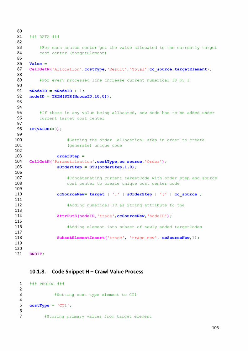
105
80 ### DATA ### 81 82
#For each source center get the value allocated to the currently target 83 cost center (targetElement) 84
85 Value = 86 CellGetN('Allocation',costType,'Result','Total',cc_source,targetElement); 87 88 #For every processed line increase current numerical ID by 1 89 90 nNodeID = nNodeID + 1; 91 nodeID = TRIM(STR(NnodeID,10,0)); 92 93 94
#If there is any value being allocated, new node has to be added under 95 current target cost center 96 97
IF(VALUE<>0); 98 99
#Getting the order (allocation) step in order to create 100 (generate) unique code 101
102 orderStep = 103 CellGetN('Parametrization',costType,cc_source,'Order'); 104 sOrderStep = STR(orderStep,1,0); 105 106
#Concatenating current targetCode with order step and source 107 cost center to create unique cost center code 108
109 ccSourceNew= target | '.' | sOrderStep | ':' | cc_source ; 110 111 #Adding numerical ID as String attribute to the 112 113 AttrPutS(nodeID,'trace',ccSourceNew,'nodeID'); 114 115 #Adding element into subset of newly added targetCodes 116 117 SubsetElementInsert('trace', 'trace_new', ccSourceNew,1); 118 119 120 ENDIF; 121
10.1.8. Code Snippet H – Crawl Value Process
### PROLOG ### 1 2 #Setting cost type element to CT1 3 4 costType = 'CT1'; 5 6 #Storing primary values from target element 7

106
8 primaryParentValue = CellGetN('Tracer',target,'Primary_Value'); 9 primaryParentDriver= CellGetN('Tracer',target,'Primary_Driver'); 10 11 #Executing crawl_element process generating trace codes 12 13 executeProcess('crawler_element','level',level,'target',target); 14 15 #Pasting primary values from drilled node to its primary component 16 17 CellPutN(primaryParentValue,'Tracer','PRIMARY'|target,'Primary_Value'); 18 CellPutN(primaryParentDriver,'Tracer','PRIMARY'|target,'Secondary_Driver_Pa19 rent'); 20 CellPutN(primaryParentValue,'Tracer','PRIMARY'|target,'Value'); 21 22 targetElement = target; 23 24 #Parsing current cost center for drilling from targetCode 25 26 position = SCAN(':',targetElement); 27 while (position<>0); 28 length = LONG(targetElement); 29 targetElement = SUBST(targetElement,position+1,length-position); 30 position = SCAN(':',targetElement); 31 END; 32 33 34 ### DATA ### 35 36 Value = 37 CellGetN('Allocation',costType,'Result','Total',cc_source,targetElement); 38 IF(VALUE<>0); 39 40
#Getting the order (allocation) step in order to create 41 (generate) unique code 42
43 orderStep = 44 CellGetN('Parametrization',costType,cc_source,'Order'); 45 sOrderStep = STR(orderStep,1,0); 46 47
#Concatenating current targetCode with order step and 48 source cost center to create unique cost center code 49
50 ccSourceNew= target | '.' | sOrderStep | ':' | cc_source ; 51 52 #Inserting Value to Trace tablespace under Value element 53 54 CellPutN(Value,'Tracer',ccSourceNew,'Value'); 55 56
#Getting and setting Primary Value from Allocation under 57 Primary_Value element 58
primary = 59 CellGetN('Allocation',costType,'Result','Total',cc_source,'Prim60
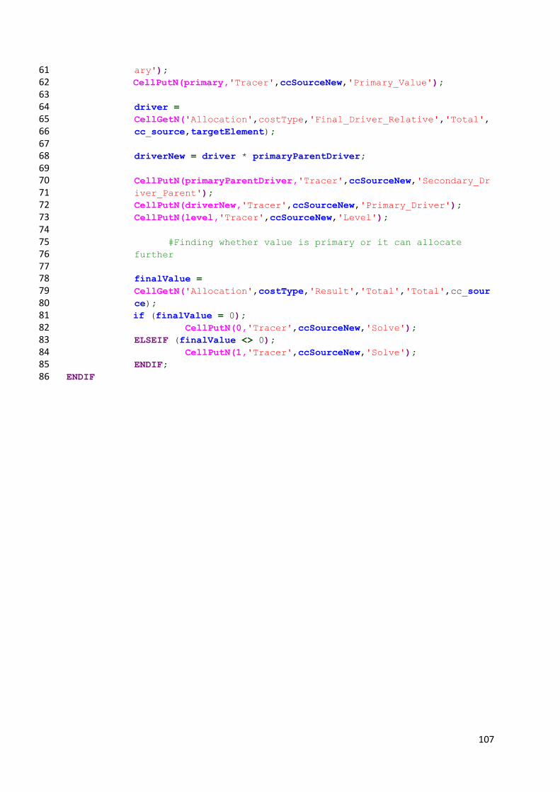
107
ary'); 61 CellPutN(primary,'Tracer',ccSourceNew,'Primary_Value'); 62
63 driver = 64 CellGetN('Allocation',costType,'Final_Driver_Relative','Total',65 cc_source,targetElement); 66
67 driverNew = driver * primaryParentDriver; 68
69 CellPutN(primaryParentDriver,'Tracer',ccSourceNew,'Secondary_Dr70 iver_Parent'); 71 CellPutN(driverNew,'Tracer',ccSourceNew,'Primary_Driver'); 72 CellPutN(level,'Tracer',ccSourceNew,'Level'); 73
74 #Finding whether value is primary or it can allocate 75
further 76 77
finalValue = 78 CellGetN('Allocation',costType,'Result','Total','Total',cc_sour79 ce); 80
if (finalValue = 0); 81 CellPutN(0,'Tracer',ccSourceNew,'Solve'); 82 ELSEIF (finalValue <> 0); 83 CellPutN(1,'Tracer',ccSourceNew,'Solve'); 84 ENDIF; 85 ENDIF86

108
11. Apendix B
11.1. Benchmarking Results
11.1.1. Hardware Performance – CPU Data in %.
Steps 5 10 Average Maximal Delta
Cost Center 80 240 480 80 240 480
Standard Average 38.6 46.6 49.7 44.8 49.4 51.0 54.5 51.1
Maximal 82.0 86.9 100,0 61.7 93.0 100,0 96.2 100,0
onDemand Average 52.2 47.3 59.9 35.2 38.1 54.4 47.8 59.9 -12.1
Maximal 35.1 90.6 100,0 47.6 56.9 100,0 71.7 100,0 -25.4

109
11.1.2. Algorithm Performance – Full Load Data in different units.
Steps S 5 10 Average Delta
Units U 80 240 480 80 240 480
Target F 17 32 48 59 96 117 9 18 24 45 48 79
Trace
TS standard 255 480 720 885 1 440 1 755 4 599 9 198 12 264 22 995 24 528 40 369 TD onDemand 68 017 128 032 964 080 1 185 015 2 616 576 3 188 952 38 250 76 500 170 424 319 545 614 880 1 011 990
Volume (kB) V
standard 52 53 158 158 317 316 135 144 373 422 825 846 onDemand 1 142 2 150 87 504 107 557 245 088 298 701 3 456 6 912 16 296 30 555 63 792 104 991
Speed (s) S
standard 10,0 12,8 56,1 72,9 200,4 252,4 38,5 46,2 194,9 272,2 964,0 1 198,2 onDemand 863,8 1 625,9 19 423,2 23 874,4 39 679,7 48 359,6 1 026,1 2 052,2 3 097,8 5 989,0 9 463,7 15 012,7
Volume/Trace (%)
VT standard 0,2039 0,1104 0,2194 0,1785 0,2201 0,1801 0,0294 0,0157 0,0304 0,0184 0,0336 0,0210 0,1051
onDemand 0,0168 0,0168 0,0908 0,0908 0,0937 0,0937 0,0904 0,0904 0,0956 0,0956 0,1037 0,1037 0,0818 -22%
Speed/Trace (%)
ST standard 0,0390 0,0267 0,0779 0,0824 0,1392 0,1438 0,0084 0,0050 0,0159 0,0118 0,0393 0,0297 0,0516
onDemand 0,0127 0,0127 0,0201 0,0201 0,0152 0,0152 0,0268 0,0268 0,0182 0,0187 0,0154 0,0148 0,0181 -65%
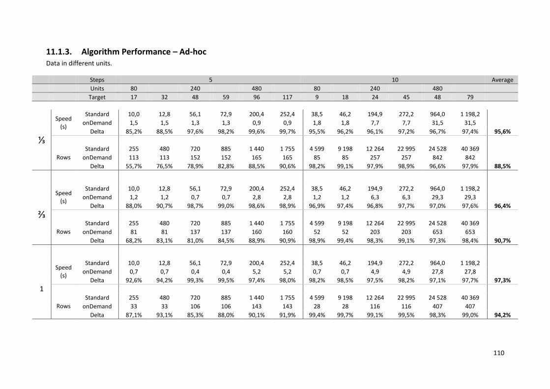
110
11.1.3. Algorithm Performance – Ad-hoc Data in different units.
Steps 5 10 Average
Units 80 240 480 80 240 480
Target 17 32 48 59 96 117 9 18 24 45 48 79
⅓
Speed (s)
Standard 10,0 12,8 56,1 72,9 200,4 252,4 38,5 46,2 194,9 272,2 964,0 1 198,2 onDemand 1,5 1,5 1,3 1,3 0,9 0,9 1,8 1,8 7,7 7,7 31,5 31,5 Delta 85,2% 88,5% 97,6% 98,2% 99,6% 99,7% 95,5% 96,2% 96,1% 97,2% 96,7% 97,4% 95,6%
Rows
Standard 255 480 720 885 1 440 1 755 4 599 9 198 12 264 22 995 24 528 40 369 onDemand 113 113 152 152 165 165 85 85 257 257 842 842 Delta 55,7% 76,5% 78,9% 82,8% 88,5% 90,6% 98,2% 99,1% 97,9% 98,9% 96,6% 97,9% 88,5%
⅔
Speed (s)
Standard 10,0 12,8 56,1 72,9 200,4 252,4 38,5 46,2 194,9 272,2 964,0 1 198,2 onDemand 1,2 1,2 0,7 0,7 2,8 2,8 1,2 1,2 6,3 6,3 29,3 29,3 Delta 88,0% 90,7% 98,7% 99,0% 98,6% 98,9% 96,9% 97,4% 96,8% 97,7% 97,0% 97,6% 96,4%
Rows
Standard 255 480 720 885 1 440 1 755 4 599 9 198 12 264 22 995 24 528 40 369 onDemand 81 81 137 137 160 160 52 52 203 203 653 653 Delta 68,2% 83,1% 81,0% 84,5% 88,9% 90,9% 98,9% 99,4% 98,3% 99,1% 97,3% 98,4% 90,7%
1
Speed (s)
Standard 10,0 12,8 56,1 72,9 200,4 252,4 38,5 46,2 194,9 272,2 964,0 1 198,2 onDemand 0,7 0,7 0,4 0,4 5,2 5,2 0,7 0,7 4,9 4,9 27,8 27,8 Delta 92,6% 94,2% 99,3% 99,5% 97,4% 98,0% 98,2% 98,5% 97,5% 98,2% 97,1% 97,7% 97,3%
Rows
Standard 255 480 720 885 1 440 1 755 4 599 9 198 12 264 22 995 24 528 40 369 onDemand 33 33 106 106 143 143 28 28 116 116 407 407 Delta 87,1% 93,1% 85,3% 88,0% 90,1% 91,9% 99,4% 99,7% 99,1% 99,5% 98,3% 99,0% 94,2%
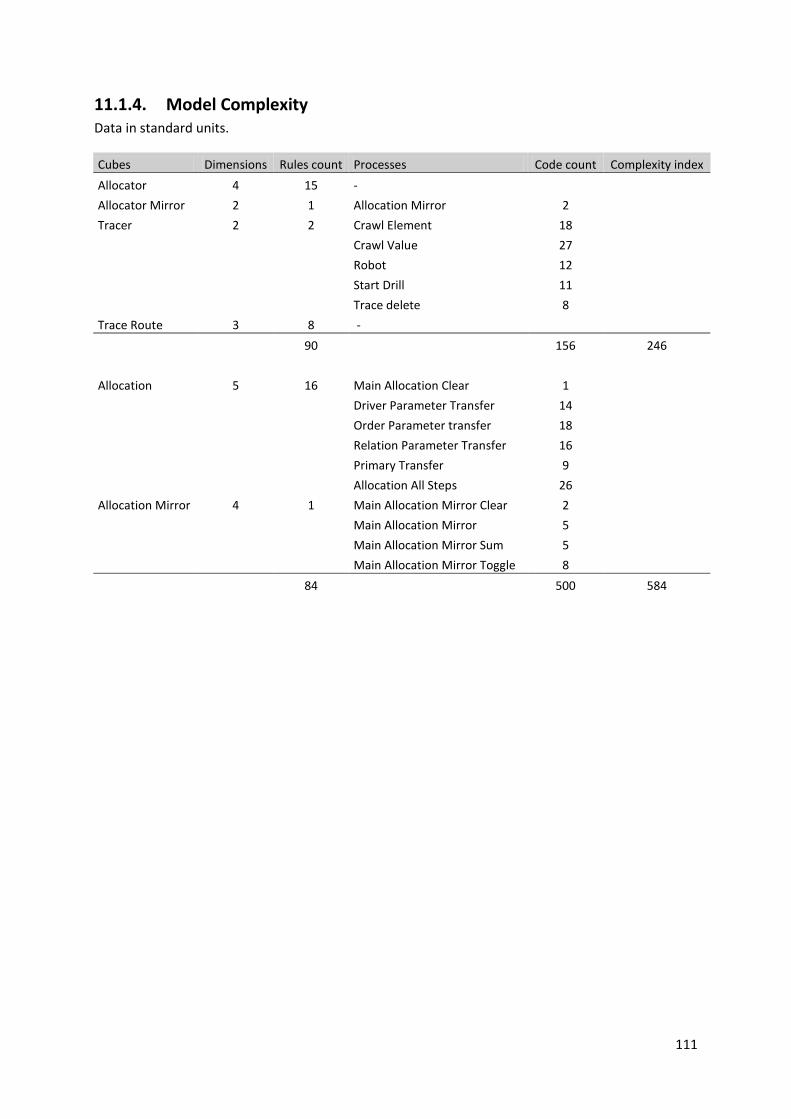
111
11.1.4. Model Complexity Data in standard units.
Cubes Dimensions Rules count Processes Code count Complexity index
Allocator 4 15 - Allocator Mirror 2 1 Allocation Mirror 2
Tracer 2 2 Crawl Element 18
Crawl Value 27
Robot 12
Start Drill 11
Trace delete 8
Trace Route 3 8 -
90
156 246
Allocation 5 16 Main Allocation Clear 1
Driver Parameter Transfer 14
Order Parameter transfer 18
Relation Parameter Transfer 16
Primary Transfer 9
Allocation All Steps 26
Allocation Mirror 4 1 Main Allocation Mirror Clear 2
Main Allocation Mirror 5
Main Allocation Mirror Sum 5
Main Allocation Mirror Toggle 8
84
500 584

112
12. Appendix C
12.1. Code Snippets
12.1.1. Code Snippet I – executeProcess function / api.php
<?php 1 2 //Array with TM1RunTI.exe error codes 3 $error = array( 4 0=>"OK", 5 1=>"Password not specified", 6 2=>"Server connection failed", 7 3=>"Process completed with minor errors" 8 ); 9 10 11 /** 12 * 13 * Executes TM1 process handling specific API function 14 * 15 * 16 * @param $fileLocation name of the computer hosting TM1 server 17 * $server name of the TM1 server 18 * $name of the TM1 process handling specific API function 19 * $user username 20 * $password user password 21 * @returns $jsonData JSON encoded output 22 */ 23 24 function executeProcess($adminhost, $server, $process, $param, $user, 25 $password){ 26 system ("\"c:\\program files\\ibm\\cognos\\tm1\\bin64\\tm1runti.exe\" 27 tm1runti -process ".$process." ".$param." -adminhost ".$adminhost." -28 server ". $server." -user ".$user." -pwd ".$password."", $message); 29 //returns TM1 message code 30 return $message; 31 }32
12.1.2. Code Snippet J – driver.php class
<?php 1 2 //loads api functions 3 require "../api.php"; 4 5 //defines location of export files 6 $fileLocation = "http://domain/api/data/driver.txt"; 7 8 //defines adminhost 9

113
$adminhost = "cognosdemo"; 10 11 //defines TM1 server 12 $server = "api"; 13 14 //defines username 15 $user = "admin"; 16 17 //defines password 18 $password = "apple"; 19 20 //gets server method issued by client 21 $method = $_SERVER['REQUEST_METHOD']; 22 23 24 //claers file 25 clearFile($fileLocation); 26 27 //executes request 28 executeRequest($method, $fileLocation, $error, $adminhost, $server, 29 $process, $user, $password); 30 31 /** 32 * 33 * Clears file before export 34 * 35 * @param $fileLocation location of file with exported data 36 */ 37 38 function clearFile($fileLocation){ 39 file_put_contents($fileLocation,""); 40 } 41 42 /** 43 * 44 * Depending on REQUEST_METHOD function executes different processes 45 * 46 * @param $method HTTP method issed by client 47 */ 48 49 function executeRequest($method, $fileLocation, $error, $adminhost, 50 $server, $process, $user, $password){ 51 switch ($method){ 52 case "GET": 53 $process = "exportCubeDriver"; 54 $param = ""; 55 $message = executeProcess($adminhost, $server, 56 $process, $param, $user, $password); 57 //issue message if any error occured 58 if ($message!=0){ 59 header("HTTP/1.1 500 Internal Server Error"); 60 print($error[$message]); 61 } 62 else { 63 $data = getData($fileLocation); 64 echo $data; 65 } 66 break; 67 } 68 } 69

114
12.1.3. Code Snippet K – getData function / api.php
<?php 1 /** 2 * 3 * Reads exported data and finishes encoding into JSON 4 * 5 * 6 * @param $fileLocation location of the file with exported data 7 * @returns $jsonData JSON encoded output 8 */ 9 10 function getData($fileLocation){ 11 $lines = file($fileLocation); 12 $jsonData = '['; 13 foreach ($lines as $line) { 14 $jsonData = $jsonData.$line; 15 } 16 $jsonData = $jsonData.']'; 17 return $jsonData; 18 } 19
12.1.4. Code Snippet L – AJAX GET method
$(document).ready(function(){ 1 $.ajax({ 2 type: 'GET'; 3 url: 'http://domain/api/cube/driver, 4 dataType: 'json'; 5 success: function(data){ 6 $.each(data, function(key, value){ 7 //process values 8 }) 9 }, 10 error: function(xhr, err){ 11 alert(xhr.responseText); 12 } 13 14 }); 15 });16
12.1.5. Code Snippet M – AJAX POST method
$(document).ready(function(){ 1 $.ajax({ 2 type: 'POST'; 3 url: 'http://domain/api/cube/driver, 4 data: {param:value} 5 dataType: 'json'; 6 success: function(message){ 7 alert(message); 8 }, 9 error: function(xhr, err){ 10
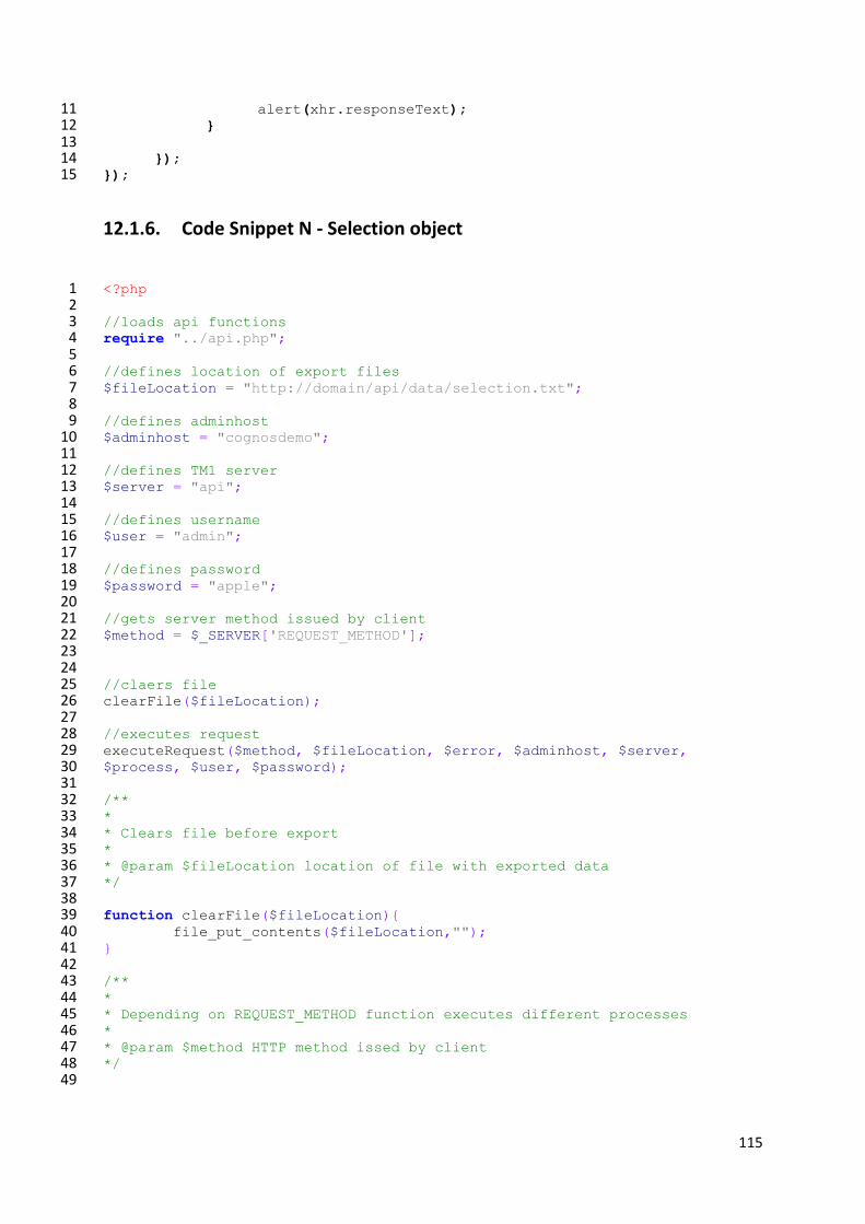
115
alert(xhr.responseText); 11 } 12 13 }); 14 }); 15
12.1.6. Code Snippet N - Selection object
<?php 1 2 //loads api functions 3 require "../api.php"; 4 5 //defines location of export files 6 $fileLocation = "http://domain/api/data/selection.txt"; 7 8 //defines adminhost 9 $adminhost = "cognosdemo"; 10 11 //defines TM1 server 12 $server = "api"; 13 14 //defines username 15 $user = "admin"; 16 17 //defines password 18 $password = "apple"; 19 20 //gets server method issued by client 21 $method = $_SERVER['REQUEST_METHOD']; 22 23 24 //claers file 25 clearFile($fileLocation); 26 27 //executes request 28 executeRequest($method, $fileLocation, $error, $adminhost, $server, 29 $process, $user, $password); 30 31 /** 32 * 33 * Clears file before export 34 * 35 * @param $fileLocation location of file with exported data 36 */ 37 38 function clearFile($fileLocation){ 39 file_put_contents($fileLocation,""); 40 } 41 42 /** 43 * 44 * Depending on REQUEST_METHOD function executes different processes 45 * 46 * @param $method HTTP method issed by client 47 */ 48 49
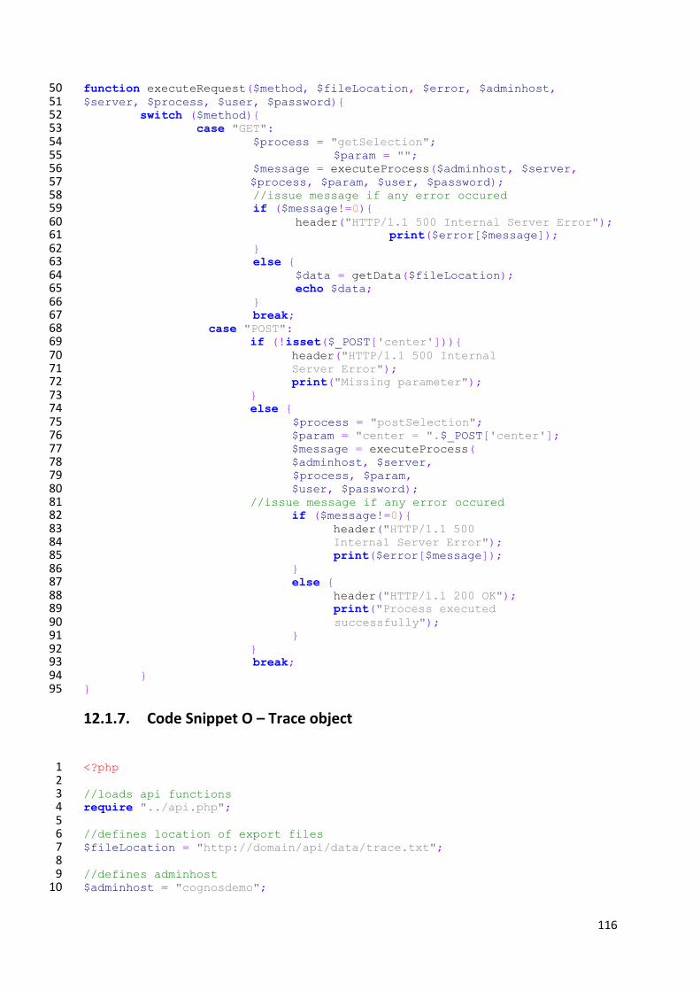
116
function executeRequest($method, $fileLocation, $error, $adminhost, 50 $server, $process, $user, $password){ 51 switch ($method){ 52 case "GET": 53 $process = "getSelection"; 54 $param = ""; 55 $message = executeProcess($adminhost, $server, 56 $process, $param, $user, $password); 57 //issue message if any error occured 58 if ($message!=0){ 59 header("HTTP/1.1 500 Internal Server Error"); 60 print($error[$message]); 61 } 62 else { 63 $data = getData($fileLocation); 64 echo $data; 65 } 66 break; 67 case "POST": 68 if (!isset($_POST['center'])){ 69 header("HTTP/1.1 500 Internal 70 Server Error"); 71 print("Missing parameter"); 72 } 73 else { 74 $process = "postSelection"; 75 $param = "center = ".$_POST['center']; 76 $message = executeProcess( 77 $adminhost, $server, 78 $process, $param, 79 $user, $password); 80 //issue message if any error occured 81 if ($message!=0){ 82 header("HTTP/1.1 500 83 Internal Server Error"); 84 print($error[$message]); 85 } 86 else { 87 header("HTTP/1.1 200 OK"); 88 print("Process executed 89 successfully"); 90 } 91 } 92 break; 93 } 94 } 95
12.1.7. Code Snippet O – Trace object
<?php 1 2 //loads api functions 3 require "../api.php"; 4 5 //defines location of export files 6 $fileLocation = "http://domain/api/data/trace.txt"; 7 8 //defines adminhost 9 $adminhost = "cognosdemo"; 10

117
11 //defines TM1 server 12 $server = "api"; 13 14 //defines username 15 $user = "admin"; 16 17 //defines password 18 $password = "apple"; 19 20 //gets server method issued by client 21 $method = $_SERVER['REQUEST_METHOD']; 22 23 24 //claers file 25 clearFile($fileLocation); 26 27 //executes request 28 executeRequest($method, $fileLocation, $error, $adminhost, $server, 29 $process, $user, $password); 30 31 /** 32 * 33 * Clears file before export 34 * 35 * @param $fileLocation location of file with exported data 36 */ 37 38 function clearFile($fileLocation){ 39 file_put_contents($fileLocation,""); 40 } 41 42 /** 43 * 44 * Depending on REQUEST_METHOD function executes different processes 45 * 46 * @param $method HTTP method issed by client 47 */ 48 49 function executeRequest($method, $fileLocation, $error, $adminhost, 50 $server, $process, $user, $password){ 51 switch ($method){ 52 case "GET": 53 $process = "getTrace"; 54 $param = ""; 55 $message = executeProcess($adminhost, $server, 56 $process, $param, $user, $password); 57 //issue message if any error occured 58 if ($message!=0){ 59 header("HTTP/1.1 500 Internal Server Error"); 60 print($error[$message]); 61 } 62 else { 63 $data = getData($fileLocation); 64 echo $data; 65 } 66 break; 67 case "POST": 68 if (!isset($_POST['code'])){ 69 header("HTTP/1.1 500 Internal 70 Server Error"); 71

118
print("Missing parameter"); 72 } 73 else { 74 $process = "postTrace"; 75 $param = "postTrace = ".$_POST['code']; 76 $message = executeProcess($adminhost, $server, 77 $process, $param, $user, $password); 78 //issue message if any error occured 79 if ($message!=0){ 80 header("HTTP/1.1 500 Internal Server 81 Error"); 82 print($error[$message]); 83 } 84 else { 85 $data = getData($fileLocation); 86 echo $data; 87 } 88 } 89 break; 90 } 91 } 92 93
13. Appendix D
13.1. Code Snippets
13.1.1. Code Snippet P – Invoke allocation
//Listener for allocate-button starts sequence of API functions 1 $(document).ready(function(){ 2 $("#allocate-button").click(function(){ 3 //gets the name of the selected center from list box 4 $center = $("#selection-list option:selected").html(); 5 postSelection($center); 6 //temporary disables allocate-button 7 $("#allocate-button").attr("disabled","disabled"); 8 }); 9 }); 10 11 /** 12 * 13 * Function executes API call to Selection cube invoked with POST method 14 * Function writes selected center into Selection cube 15 * 16 * @param $center name of the selected center 17 */ 18 function postSelection($center){ 19 $.ajax({ 20 type: 'POST', 21 url:'http://domain/api/cube/selection', 22 data: {center:$center}, 23 dataType: 'json', 24 success: function(data){ 25
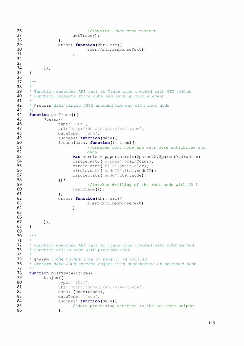
119
//invokes Trace cube restart 26 getTrace(); 27 }, 28 error: function(xhr, err){ 29 alert(xhr.responseText); 30 } 31 32 33 }); 34 } 35 36 /** 37 * 38 * Function executes API call to Trace cube invoked with GET method 39 * Function restarts Trace cube and sets up root element 40 * 41 * @return data single JSON encoded element with root node 42 */ 43 function getTrace(){ 44 $.ajax({ 45 type: 'GET', 46 url:'http://domain/api/view/trace', 47 dataType: 'json', 48 success: function(data){ 49 $.each(data, function(i, item){ 50 //creates root node and sets core attributes and 51 data 52 var circle = paper.circle($parentX,$parentY,$radius); 53 circle.attr("stroke",$mainColor); 54 circle.attr("fill",$mainColor); 55 circle.data("nodeID",item.nodeID); 56 circle.data("node",item.node); 57 }); 58 //invokes drilling of the root node with ID 1 59 postTrace(1); 60 }, 61 error: function(xhr, err){ 62 alert(xhr.responseText); 63 } 64 65 66 }); 67 } 68 69 /** 70 * 71 * Function executes API call to Trace cube invoked with POST method 72 * Function drills node with provided code 73 * 74 * @param $code unique code of node to be drilled 75 * $return data JSON encoded object with descendants of selected node 76 */ 77 function postTrace($code){ 78 $.ajax({ 79 type: 'POST', 80 url:'http://domain/api/view/trace', 81 data: {code:$code}, 82 dataType: 'json', 83 success: function(data){ 84 //data processing attached in the nex code snippet 85 }, 86

120
error: function(xhr, err){ 87 alert(xhr.responseText); 88 } 89 90 91 }); 92 }93
13.1.2. Code Snippet Q –Comparison tree processing on received data
.success(function(data){ 1 $("#block").remove(); 2 $.each(data, function(i, item){ 3 //generates appropriate random X position for current 4 node 5 $left = getXPosition(item, $nodeID); 6 //genrates appropraite random Y position for current node 7 $top = getYPosition(item); 8 //skips primary cost values 9 if (item.type!=0){ 10 //creates new node and assigns core attributes 11 $circle = createNode(item, $left, $top); 12 //click listener implementation 13 $circle.click(function(){ 14 //removes node in case remove checkbox is checked 15 if($("#remove").is(":checked")){removeNode(this);} 16 else { 17 //assigns additional actions when item 18 is still drilable 19 if (item.solve==1){ 20 //invoke drilling when node has 21 not been drilled yet 22 23 if(this.data("open")!=1){ 24 invokeDrill(this);} 25 //otherwise change visibility 26 else {changeVisibility(this);} 27 } 28 } 29 }); 30 } 31 //hove listener implementation 32 $circle.hover( 33 //adds hover actions 34 function(){hover(this);}, 35 //adds unhover actions 36 function(){unhover(this);} 37 ); 38 }); 39 //recolors all nodes based on the color palett 40 recolorAllLevels(); 41 //bounce overlaying nodes 42 bounceCircle(); 43 }) 44 .error(function(xhr,err){ 45 $("#block").remove(); 46 alert(xhr.responseText); 47

121
}); 48
13.1.3. Code Snippet R – Invoke drill function
/** 1 * 2 * Function calls function executing API request to Trace cube with POST 3 method 4 * Function drills node with provided code 5 * 6 * @param $this context of clicked object 7 */ 8 function invokeDrill($this){ 9 //enlarges the node 10 $this.animate({r:$radiusBig},$speed); 11 $nodeID = $this.data("nodeID"); 12 postTrace($nodeID); 13 //sets up global parameters for parent's position 14 $parentX = $this.attr("cx"); 15 $parentY = $this.attr("cy"); 16 //marks node as opened 17 $this.data("open",1); 18 } 19
13.1.4. Code Snippet S – Change visibility function
/** 1 * 2 * Function changes visibility of all node's descentants 3 * 4 * @param $this context of clicked object 5 */ 6 function changeVisibility($this){ 7 $nodeID = $this.data("nodeID"); 8 $parentNodeID = $this.data("parentNodeID"); 9 if ($this.data("close")!=1){ 10 hide($nodeID); 11 unconnect($nodeID); 12 unconnectParent($parentNodeID); 13 $this.data("close",1); 14 $this.animate({r:$radiusSmall},$speed); 15 $this.resume(); 16 } 17 else { 18 show($nodeID); 19 connect($this.attr("cx"),$this.attr("cy"),$nodeID); 20 bounceCircle(); 21 $this.data("close",0); 22 $this.pause(); 23 $this.animate({r:radiusBig},$speed); 24 } 25 } 26
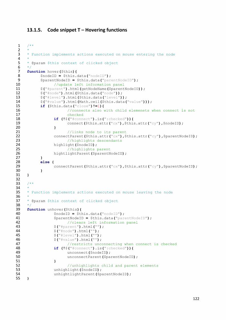
122
13.1.5. Code snippet T – Hovering functions
/** 1 * 2 * Function implements actions executed on mouse entering the node 3 * 4 * @param $this context of clicked object 5 */ 6 function hover($this){ 7 $nodeID = $this.data("nodeID"); 8 $parentNodeID = $this.data("parentNodeID"); 9 //update left information panel 10 $("#parent").html(getNodeName($parentNodeID)); 11 $("#node").html($this.data("node")); 12 $("#level").html($this.data("level")); 13 $("#value").html(Math.ceil($this.data("value"))); 14 if ($this.data("close")!=1){ 15 //connects also with child elemenets when connect is not 16 checked 17 if (!$("#connect").is(":checked")){ 18 connect($this.attr("cx"),$this.attr("cy"),$nodeID); 19 } 20 //links node to its parent 21 connectParent($this.attr("cx"),$this.attr("cy"),$parentNodeID); 22 //highlights descendants 23 highlight($nodeID); 24 //highlights parent 25 hightlightParent($parentNodeID); 26 } 27 else { 28 connectParent($this.attr("cx"),$this.attr("cy"),$parentNodeID); 29 } 30 } 31 32 /** 33 * 34 * Function implements actions executed on mouse leaving the node 35 * 36 * @param $this context of clicked object 37 */ 38 function unhover($this){ 39 $nodeID = $this.data("nodeID"); 40 $parentNodeID = $this.data("parentNodeID"); 41 //clears left information panel 42 $("#parent").html(""); 43 $("#node").html(""); 44 $("#level").html(""); 45 $("#value").html(""); 46 //restricts unconnecting when connect is checked 47 if (!$("#connect").is(":checked")){ 48 unconnect($nodeID); 49 unconnectParent($parentNodeID); 50 } 51 //unhighlights child and parent elements 52 unhighlight($nodeID); 53 unhightlightParent($parentNodeID); 54 } 55
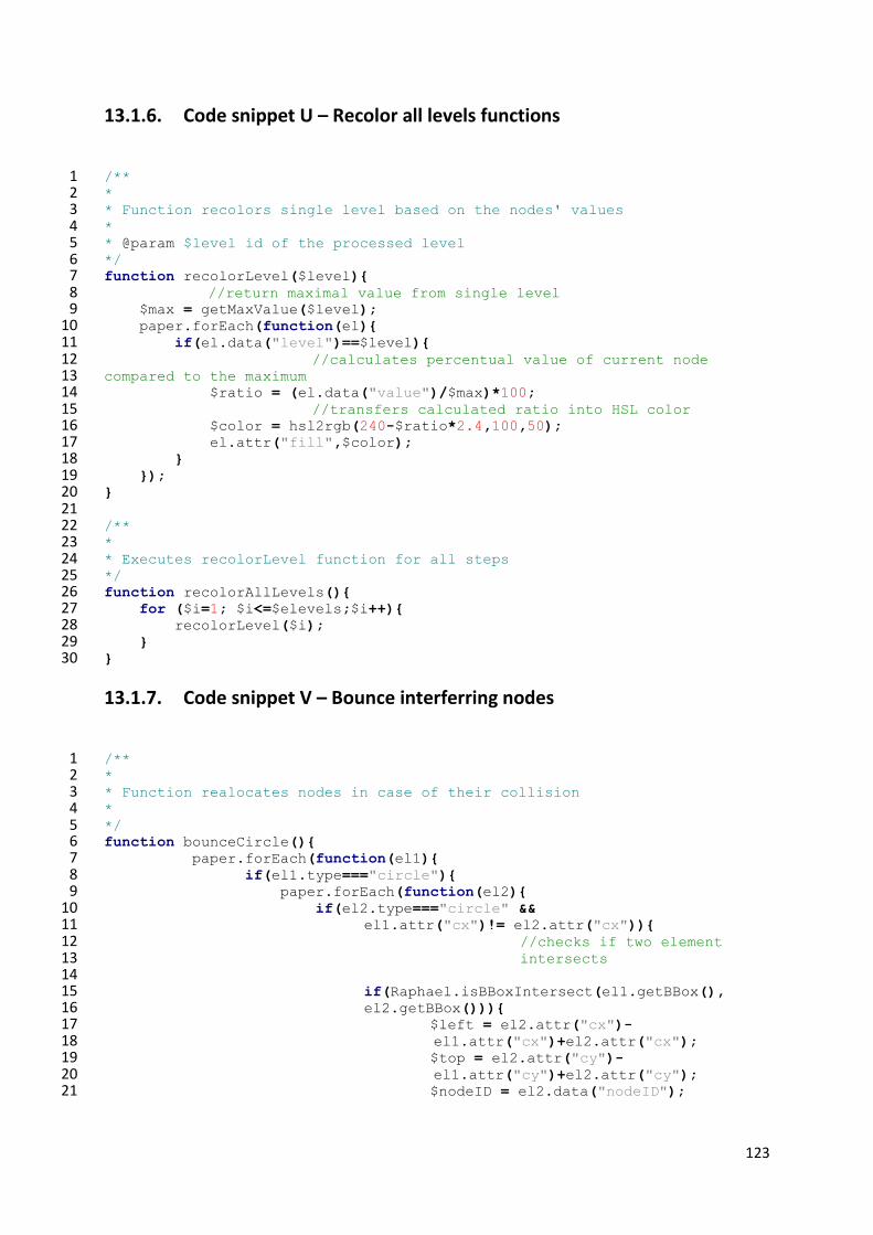
123
13.1.6. Code snippet U – Recolor all levels functions
/** 1 * 2 * Function recolors single level based on the nodes' values 3 * 4 * @param $level id of the processed level 5 */ 6 function recolorLevel($level){ 7 //return maximal value from single level 8 $max = getMaxValue($level); 9 paper.forEach(function(el){ 10 if(el.data("level")==$level){ 11 //calculates percentual value of current node 12 compared to the maximum 13 $ratio = (el.data("value")/$max)*100; 14 //transfers calculated ratio into HSL color 15 $color = hsl2rgb(240-$ratio*2.4,100,50); 16 el.attr("fill",$color); 17 } 18 }); 19 } 20 21 /** 22 * 23 * Executes recolorLevel function for all steps 24 */ 25 function recolorAllLevels(){ 26 for ($i=1; $i<=$elevels;$i++){ 27 recolorLevel($i); 28 } 29 } 30
13.1.7. Code snippet V – Bounce interferring nodes
/** 1 * 2 * Function realocates nodes in case of their collision 3 * 4 */ 5 function bounceCircle(){ 6 paper.forEach(function(el1){ 7 if(el1.type==="circle"){ 8 paper.forEach(function(el2){ 9 if(el2.type==="circle" && 10 el1.attr("cx")!= el2.attr("cx")){ 11 //checks if two element 12 intersects 13 14 if(Raphael.isBBoxIntersect(el1.getBBox(), 15 el2.getBBox())){ 16 $left = el2.attr("cx")- 17 el1.attr("cx")+el2.attr("cx"); 18 $top = el2.attr("cy")- 19 el1.attr("cy")+el2.attr("cy"); 20 $nodeID = el2.data("nodeID"); 21

124
//animates reposition of both 22 nodes using elastic movement 23 var bounceBall = Raphael.animation( 24 {cx:$left,cy:$top},100,'elastic', 25 function(){bounceCircle();}); 26 el2.animate(bounceBall); 27 } 28 } 29 }); 30 } 31 }); 32 } 33
13.1.8. Code snippet X – Drill-down ad-hoc processing of received data
.success(function(data){ 1 $("#block").remove(); 2 $.each(data, function(i, item){ 3 $position = generatePosition(item); 4 $left = $position[0]; 5 $top = $position[1]; 6 createPath($left, $top, item.nodeID, 7 item.parentNodeID,$speedSlow,0); 8 $circle = createCircle($left, $top, $radius, item.nodeID, 9 item.node, item.parentNodeID, item.level, item.value, 10 $speedFast, 0); 11 if (item.solve==1){ 12 $circle.click(function(){ 13 if (this.data("center")!=1){ 14 if (this.data("open")==0){ 15 focusNode(this); 16 $nodeID = this.data("nodeID"); 17 postTrace($nodeID); 18 this.data("open",1); 19 } 20 else { 21 focusNode(this); 22 $nodeID = this.data("nodeID"); 23 reopenNode($nodeID); 24 } 25 } 26 else { 27 closeNodes(); 28 deofsetCenter(); 29 showElements(); 30 this.data("center",0); 31 } 32 }); 33 } 34 else { 35 $circle.attr("fill","silver"); 36 } 37 recolorAllLevels(); 38 }); 39 }) 40 .error(function(xhr,err){ 41 $(".loading").remove(); 42 alert(xhr.responseText); 43
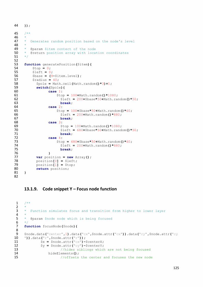
125
}); 44
/** 45 * 46 * Generates random position based on the node's level 47 * 48 * @param $item contect of the node 49 * @return position array with location coordinates 50 */ 51 52 function generatePosition($item){ 53 $top = 0; 54 $left = 0; 55 $base = (9-$item.level); 56 $radius = 40; 57 $pole = Math.ceil(Math.random()*3)+1; 58 switch($pole){ 59 case 1: 60 $top = 100+Math.random()*1080; 61 $left = 200+$base*50+Math.random()*50; 62 break; 63 case 2: 64 $top = 100+$base*50+Math.random()*60; 65 $left = 200+Math.random()*880; 66 break; 67 case 3: 68 $top = 100+Math.random()*1080; 69 $left = 680+$base*50+Math.random()*50; 70 break; 71 case 4: 72 $top = 680+$base*50+Math.random()*60; 73 $left = 200+Math.random()*880; 74 break; 75 } 76 var position = new Array(); 77 position[0] = $left; 78 position[1] = $top; 79 return position; 80 } 81 82
13.1.9. Code snippet Y – Focus node function
/** 1 * 2 * Function simulates focus and transition from higher to lower layer 3 * 4 * @param $node node which is being focused 5 */ 6 function focusNode($node){ 7 8 $node.data("center",1).data("cx",$node.attr("cx")).data("cy",$node.attr("cy9 ")).data("r",$node.attr("r")); 10 $x = $node.attr("cx")-$centerX; 11 $y = $node.attr("cy")-$centerY; 12 //hides siblings which are not being focused 13 hideElements(); 14 //offsets the center and focuses the new node 15
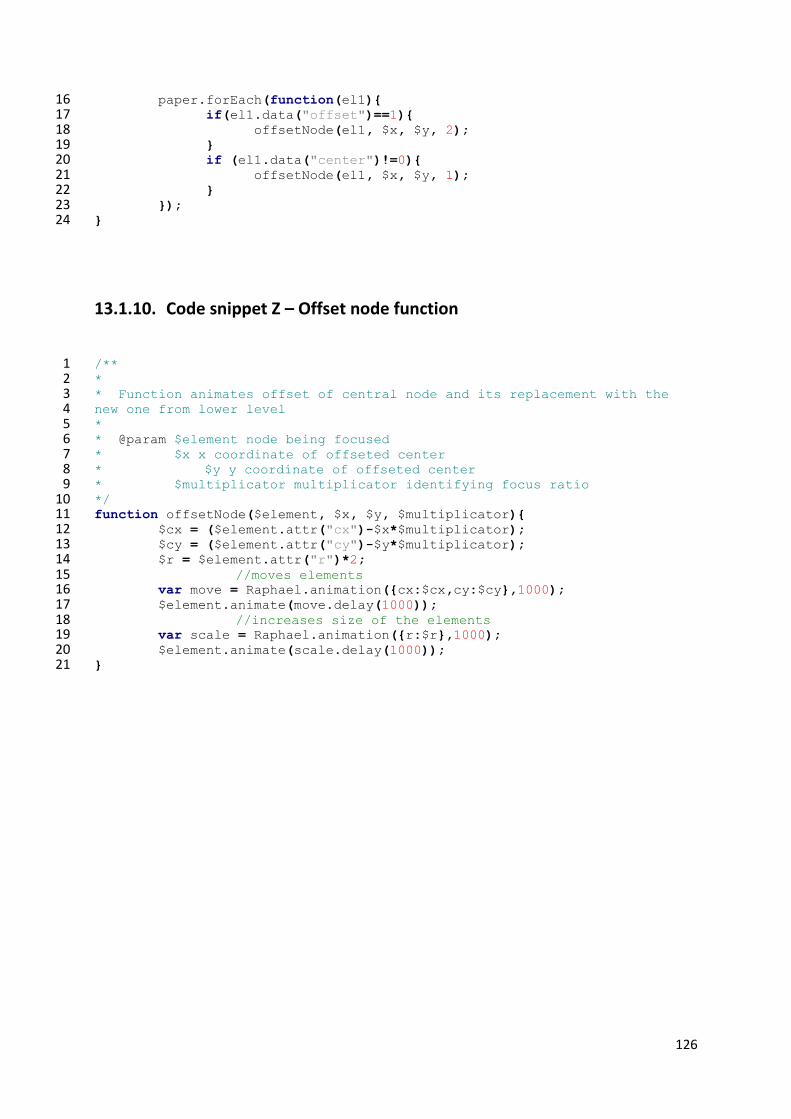
126
paper.forEach(function(el1){ 16 if(el1.data("offset")==1){ 17 offsetNode(el1, $x, $y, 2); 18 } 19 if (el1.data("center")!=0){ 20 offsetNode(el1, $x, $y, 1); 21 } 22 }); 23 } 24
13.1.10. Code snippet Z – Offset node function
/** 1 * 2 * Function animates offset of central node and its replacement with the 3 new one from lower level 4 * 5 * @param $element node being focused 6 * $x x coordinate of offseted center 7 * $y y coordinate of offseted center 8 * $multiplicator multiplicator identifying focus ratio 9 */ 10 function offsetNode($element, $x, $y, $multiplicator){ 11 $cx = ($element.attr("cx")-$x*$multiplicator); 12 $cy = ($element.attr("cy")-$y*$multiplicator); 13 $r = $element.attr("r")*2; 14 //moves elements 15 var move = Raphael.animation({cx:$cx,cy:$cy},1000); 16 $element.animate(move.delay(1000)); 17 //increases size of the elements 18 var scale = Raphael.animation({r:$r},1000); 19 $element.animate(scale.delay(1000)); 20 } 21