cycle time improvement by a six sigma project for the

International Journal of Industrial Engineering, 16(3), 191-205, 2009.

ISSN 1943-670X © INTERNATIONAL JOURNAL OF INDUSTRIAL ENGINEERING

Cycle Time Improvement by a Six Sigma Project for the Increase of New

Business Accounts

M. White1, J. L. García

1, J. A. Hernández

1, and J. Meza

2

1Department of Industrial and Manufacturing Engineering

Institute of Engineering and Technology Autonomous University of Ciudad Juarez

2Department of Industrial Engineering Colima Institute of Technology

Corresponding author: {Jorge L. Garcia A., [email protected]}

This paper reports the application of a 6σ project about the reduction of the cycle time for acquiring a new credit account in a finance group. The methodology used in this project was the DMAI technique of 6σ. The paper documents the analysis and tasks performed by the management team that reduced cycle time from 49 days to 30 days which resulted in an expected annual savings of $300,000.00. Also an increased customer satisfaction and an increase of sales is expected. Significance: The 6σ literature of industrial applications is extensive, but the services applications are somewhat difficult

to find. This paper is important because it presents an application of a technique used traditionally in manufacturing industries in a service process.

Keywords: Cycle time reduction, six sigma services improvement.

(Received: 14 October 2008; Accepted in revised form: 18 May 2009)

1. INTRODUCTION

Six Sigma was conceived as a technique focused to reduce waste due to process inefficiencies in manufacturing, and for quality improvement in a product; nevertheless it is now used by almost all industries including service industries such as health care management. This is due to successful implantation programs (Krupar, 2003; Antony, 2004; Antony and Fergusson, 2004; Moorman, 2005; Frings and Grant, 2005; Kumar et al., 2008). Nevertheless, the industrial applications have had a better diffusion. The literature is replete with many applications and success cases studies in different companies using projects applying six sigma and any technique from it. Table 3 illustrates the metric used to measure the impact and success and the approximation of savings for financial institutions. Table 3 also demonstrates the results and findings obtained by Motorola, Raytheon/Aircraft Integration System and General Electric, pioneers in six sigma application, implantation, and diffusion (Kumar et al., 2008; Kwak and Anbari, 2006; Weiner, 2004; De Feo and Bar-El, 2002; Antony and Banuelas, 2002; Buss and Ivey, 2001; McClusky, 2000; Anon, 2007a,b). The typical financial six sigma projects include improving accuracy of allocation of cash to reduce bank charges, improving the efficiency of automatic payments, improving accuracy of reporting, reducing documentation, reducing the number of credits defects, reducing check collection defects, and reducing variation in collector performance (Kwak and Ambari, 2006). Specifically Bank of America (BOA) is one of the pioneers in adopting and implementing six sigma projects that are focused to streamline operations, attract new and retain current customers, and creates competitiveness and productivity over credit unions. An important data is that BOA reported a 10.4% increase in customer satisfaction and 24% decrease in customer problems after implementing six sigma (Roberts 2004, Kwak and Ambari 2006). Another financial institution applying six sigma processes is American Express. The main results were an improvement in external vendor processes, elimination of non-received renewal credit cards, and an improved sigma level of 0.3 in each case (Bolt et al., 2000; Kwak and Anbari, 2006). GE Capital Corp., JP Morgan Chase, and SunTrust Banks are applying six sigma to improve customer requirements and satisfaction (Roberts 2004, Kwak and Anbari 2006).

The objective of this paper is to report the experience and results of a financial company in applying six sigma methodologies for reducing the cycle time for approval/disapproval of credit for a new customer. The average time was originally 49 days. This was reduced to only 30 days for customers that represent 80% of the business for loans less than $100,000 dollars

White et al.

192

2. METHODOLOGY The methodology (Table 1) for the six sigma application for this company was the DMAIC (Define, Measure, Analyze, Improve and Control) process (McClusky, 2000; Kwak and Anbari, 2006). The main steps and its activities are defined in the next paragraphs.

Table 1. Methodology for Six Sigma

Steps in Six Sigma Main Activities

Define

Define the requirements and expectations of the customer. Define the project boundaries establishing some goal and objectives. Define the process by mapping the business flow, separating the job in its components for future analysis

Measure

Measure the process to satisfy customer’s needs Develop a data collection plan and metrics Collect and compare data to determine issues and shortfalls

Analyze

Analyze the causes of defects and sources of variation. Fishbone graph, correlation analysis. Determine the variations in the process. Prioritize opportunities for future improvement ranking the most important and with better impact.

Improve Improve the process to eliminate variations Develop creative alternatives and implement enhanced plan

Control Control process variations to meet customer requirements Develop a strategy to monitor and control the improved process Implement the improvements of systems and structures

3. SIX SIGMA PROJECT The results and findings are reported according to six sigma steps defined in table 1. Findings are reported in the following sub-paragraphs.

3.1. Define The financial company where this project was applied operates in 24 states in the USA with three geographic divisions, West, East and Central. The main activity is the financing of loans to diverse types of clients. The company’s main problem that there was an average of 49 days for approval or rejection of a loan application. Not only is this is unacceptably long for customers but it represents a strategic disadvantage for the bank. This disadvantage is due to the average time that competition can be projected is only 30 days. So, the main objective of this project was to reduce the time for opening a new loan account would be reduced fom 45 to 30 days.

>$250,000< $100,000$100,000>$250,000

140

120

100

80

60

40

20

0

sub

Stack

Figure 1. Amount of Credit and its Average Time

Frequency

Percent

Loan AmountCount

80.0 95.7 100.0

1005 198 54

Percent 80.0 15.8 4.3

Cum %

Other100,000-250,000<100,000

1400

1200

1000

800

600

400

200

0

100

80

60

40

20

0

Figure 2. Loans and its Frecuency in 2007

Cycle Time Improvement by a Six Sigma Project

193

The company classifies the loans granted based on the amount of money demanded. One would hope that a greater amount of credit would correspond to a longer approval time, due mainly to more information required. Nevertheless, figure 1 illustrates that the approval time is similar in all subgroups of credits. An analysis of the amount of credits for each type has been done, and the team found that 80% of the loans requested were less than $100.000. This is the primary reason that this category was chosen for analysis (figure 2).

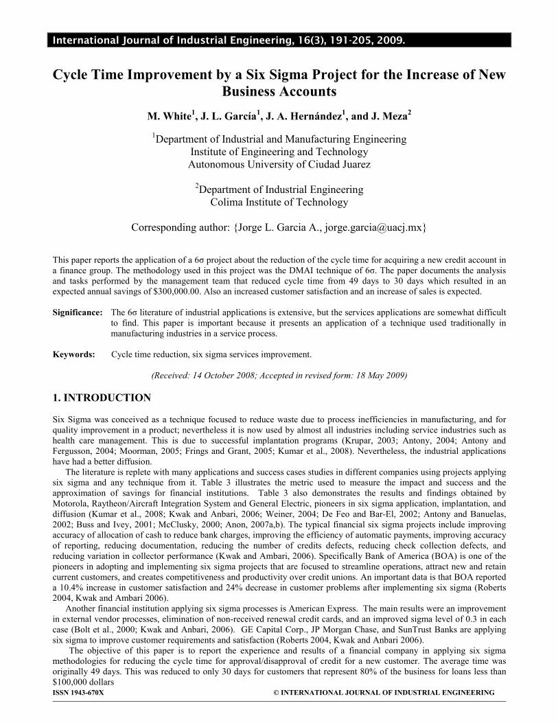
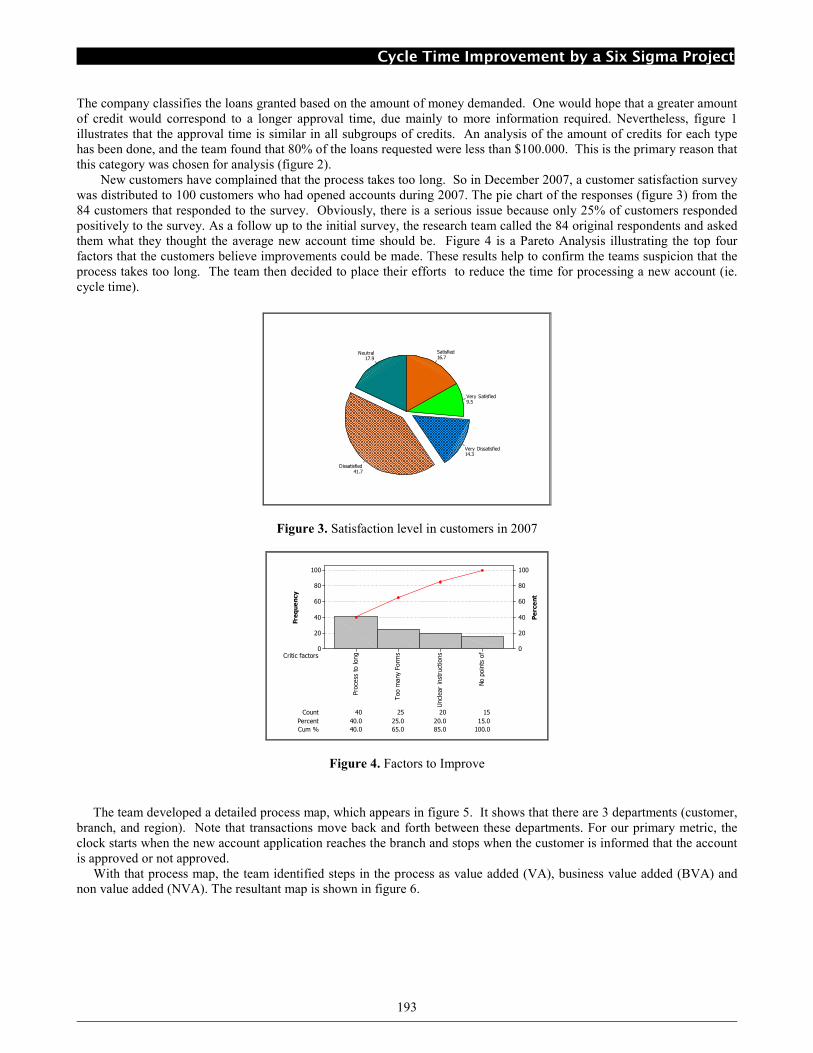
New customers have complained that the process takes too long. So in December 2007, a customer satisfaction survey was distributed to 100 customers who had opened accounts during 2007. The pie chart of the responses (figure 3) from the 84 customers that responded to the survey. Obviously, there is a serious issue because only 25% of customers responded positively to the survey. As a follow up to the initial survey, the research team called the 84 original respondents and asked them what they thought the average new account time should be. Figure 4 is a Pareto Analysis illustrating the top four factors that the customers believe improvements could be made. These results help to confirm the teams suspicion that the process takes too long. The team then decided to place their efforts to reduce the time for processing a new account (ie. cycle time).

17.9Neutral

41.7Dissatisfied

14.3Very Dissatisfied

9.5Very Satisfied

16.7Satisfied

Figure 3. Satisfaction level in customers in 2007

Frequency

Percent

Critic factors

Count

15.0

Cum % 40.0 65.0 85.0 100.0

40 25 20 15

Percent 40.0 25.0 20.0

No points of

Unclear instructions

Too many Forms

Process to long

100

80

60

40

20

0

100

80

60

40

20

0

Figure 4. Factors to Improve

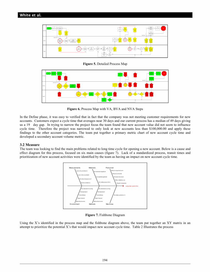
The team developed a detailed process map, which appears in figure 5. It shows that there are 3 departments (customer, branch, and region). Note that transactions move back and forth between these departments. For our primary metric, the clock starts when the new account application reaches the branch and stops when the customer is informed that the account is approved or not approved. With that process map, the team identified steps in the process as value added (VA), business value added (BVA) and non value added (NVA). The resultant map is shown in figure 6.

White et al.

194

Customer

Branch

Region

Start1

Requests Loan

2

Fills out loan application

3

Complete Application -

Preliminary Score

8Receive and

Review Application

5

Send

Application to

Region

9

Review Application

10

Score Application

13 Meets Auto

Approve Criteria?

15

Underwrite Loan

16

No

Deal Found?

17

Create Docs

18Yes

Send Docs to

Branch

19

Yes

Receive Docs

20

Send Docs to

Customer

21

Sign Docs

22 Send to

Branch

23

Review Docs

24 Send to

Region

25

Review Docs

26

Approve?

30

Send

Approval to

Branch

31

Yes

Notify

Customer of

Approval

32

Receive Notification of

Approval

33

Draw Money

34

Send Loan

Not Approved

Notice to

Branch

36

Send Loan

Not Approved

to Customer

37

No

Stop

35

Application

Complete?

6

Yes

No

Application Complete

11

Yes

No

Send back to

branch

12

Recieve Notice of Disapproval

38

No

Start Clock

Stop Clock

Acceptable Score?

14

Yes

No

Doc's OK?

27

No

Send to

Branch

28

Send to

Customer

29

Yes

Send back to

customer

7

Send to bank

4

Figure 5. Detailed Process Map

Customer

Branch

Region

Start1

Requests Loan

2

Fills out loan application

3

Complete Application -

Preliminary Score

8Receive and

Review Application

5

Send

Application to

Region

9

Review Application

10

Score Application

13 Meets Auto

Approve Criteria?

15

Underwrite Loan

16

No

Deal Found?

17

Create Docs

18Yes

Send Docs to

Branch

19

Yes

Receive Docs

20

Send Docs to

Customer

21

Sign Docs

22 Send to

Branch

23

Review Docs

24 Send to

Region

25

Review Docs

26

Approve?

30

Send

Approval to

Branch

31

Yes

Notify

Customer of

Approval

32

Receive Notification of

Approval

33

Draw Money

34

Send Loan

Not Approved

Notice to

Branch

36

Send Loan

Not Approved

to Customer

37

No

Stop

35

Application

Complete?

6

Yes

No

Application Complete

11

Yes

No

Send back to

branch

12

Recieve Notice of Disapproval

38

No

Start Clock

Stop Clock

Acceptable Score?

14

Yes

No

Doc's OK?

27

No

Send to

Branch

28

Send to

Customer

29

Yes

Send back to

customer

7

Send to bank

4

Figure 6. Process Map with VA, BVA and NVA Steps In the Define phase, it was easy to verified that in fact that the company was not meeting customer requirements for new accounts. Customers expect a cycle time that averages near 30 days and our current process has a median of 49 days giving us a 19 day gap. In trying to narrow the project focus the team found that new account value did not seem to influence cycle time. Therefore the project was narrowed to only look at new accounts less than $100,000.00 and apply these findings to the other account categories. The team put together a primary metric chart of new account cycle time and developed a secondary account volume metric.

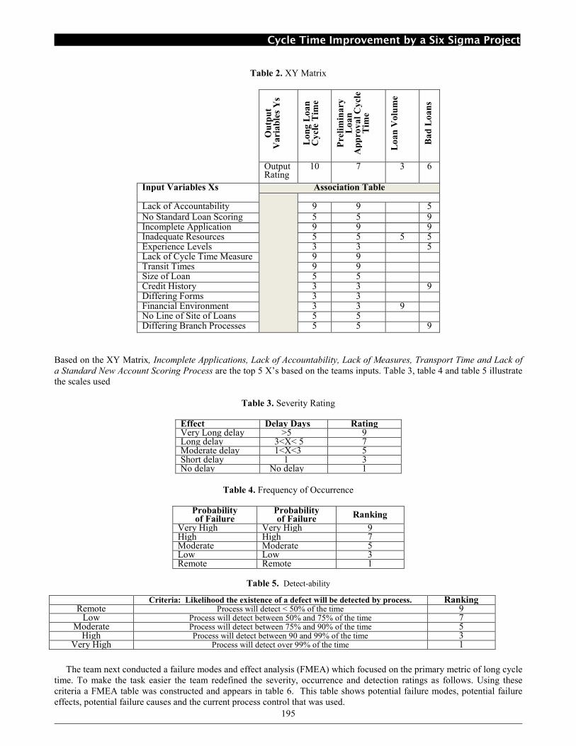
3.2 Measure The team was looking to find the main problems related to long time cycle for opening a new account. Below is a cause and effect diagram for this process, focused on six main causes (figure 7). Lack of a standardized process, transit times and prioritization of new account activities were identified by the team as having an impact on new account cycle time.

Long loan cycle time

Branch experience le

Resource levels

No team s truc ture

Other initiatives an

Time for renewals

No data sys tems or t

No s tandard applicat

Incomplete applicati

No multipurpose form

Manual process

Paper based

Transit times

Not s tandard

No s tandard scoring

Lack of cyc le time m

Lack of accountabili

No direct measure of

No line of site to c

Manual process

Paper based

Transit times

Not standard

No s tandard scoring

Personnel

Machines

Materials

Methods

Measurements

Environment

Figure 7. Fishbone Diagram Using the X’s identified in the process map and the fishbone diagram above, the team put together an XY matrix in an attempt to prioritize the potential X’s that would impact new account cycle time. Table 2 Illustrates the process


195

Table 2. XY Matrix

Output

Variables Ys

Long Loan

Cycle Time

Preliminary

Loan

Approval Cycle

Time

Loan Volume

Bad Loans

Output Rating

10 7 3 6

Input Variables Xs Association Table

Lack of Accountability 9 9 5 No Standard Loan Scoring 5 5 9 Incomplete Application 9 9 9 Inadequate Resources 5 5 5 5 Experience Levels 3 3 5 Lack of Cycle Time Measure 9 9 Transit Times 9 9 Size of Loan 5 5 Credit History 3 3 9 Differing Forms 3 3 Financial Environment 3 3 9 No Line of Site of Loans 5 5 Differing Branch Processes 5 5 9

Based on the XY Matrix, Incomplete Applications, Lack of Accountability, Lack of Measures, Transport Time and Lack of

a Standard New Account Scoring Process are the top 5 X’s based on the teams inputs. Table 3, table 4 and table 5 illustrate the scales used

Table 3. Severity Rating

Effect Delay Days Rating Very Long delay >5 9 Long delay 3<X< 5 7 Moderate delay 1<X<3 5 Short delay 1 3 No delay No delay 1

Table 4. Frequency of Occurrence

Probability of Failure

Probability of Failure

Ranking

Very High Very High 9 High High 7 Moderate Moderate 5 Low Low 3 Remote Remote 1

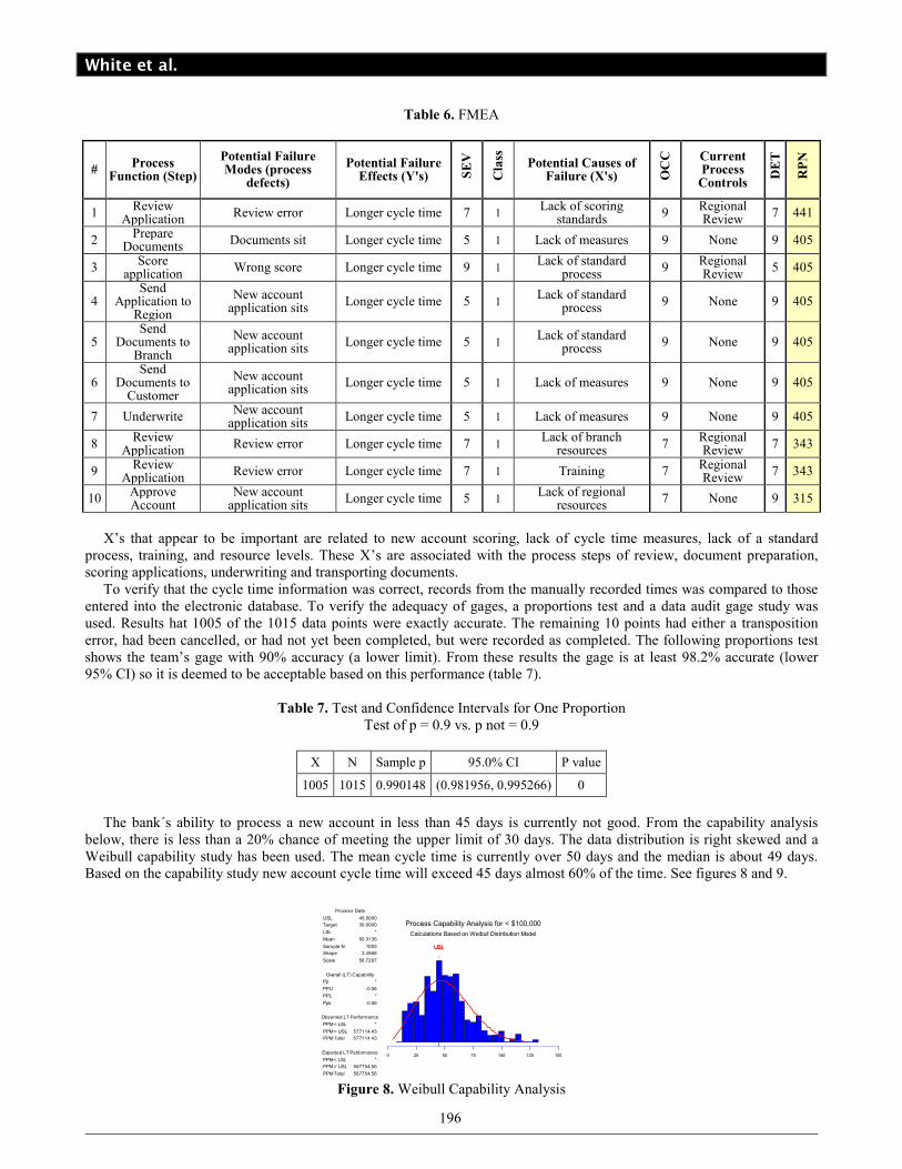
Table 5. Detect-ability

The team next conducted a failure modes and effect analysis (FMEA) which focused on the primary metric of long cycle time. To make the task easier the team redefined the severity, occurrence and detection ratings as follows. Using these criteria a FMEA table was constructed and appears in table 6. This table shows potential failure modes, potential failure effects, potential failure causes and the current process control that was used.

Criteria: Likelihood the existence of a defect will be detected by process. Ranking Remote Process will detect < 50% of the time 9

Low Process will detect between 50% and 75% of the time 7 Moderate Process will detect between 75% and 90% of the time 5

High Process will detect between 90 and 99% of the time 3 Very High Process will detect over 99% of the time 1

White et al.

196

Table 6. FMEA

# Process

Function (Step)

Potential Failure Modes (process defects)

Potential Failure Effects (Y's) S

EV

Class

Potential Causes of Failure (X's) O

CC

Current Process Controls

DET

RPN

1 Review

Application Review error Longer cycle time 7 1

Lack of scoring standards

9 Regional Review

7 441

2 Prepare

Documents Documents sit Longer cycle time 5 1 Lack of measures 9 None 9 405

3 Score

application Wrong score Longer cycle time 9 1

Lack of standard process

9 Regional Review

5 405

4 Send

Application to Region

New account application sits

Longer cycle time 5 1 Lack of standard

process 9 None 9 405

5 Send

Documents to Branch


Longer cycle time 5 1 Lack of standard

process 9 None 9 405

6 Send

Documents to Customer


Longer cycle time 5 1 Lack of measures 9 None 9 405

7 Underwrite New account

application sits Longer cycle time 5 1 Lack of measures 9 None 9 405

8 Review

Application Review error Longer cycle time 7 1

Lack of branch resources

7 Regional Review

7 343

9 Review

Application Review error Longer cycle time 7 1 Training 7

Regional Review

7 343

10 Approve Account


Longer cycle time 5 1 Lack of regional

resources 7 None 9 315

X’s that appear to be important are related to new account scoring, lack of cycle time measures, lack of a standard process, training, and resource levels. These X’s are associated with the process steps of review, document preparation, scoring applications, underwriting and transporting documents. To verify that the cycle time information was correct, records from the manually recorded times was compared to those entered into the electronic database. To verify the adequacy of gages, a proportions test and a data audit gage study was used. Results hat 1005 of the 1015 data points were exactly accurate. The remaining 10 points had either a transposition error, had been cancelled, or had not yet been completed, but were recorded as completed. The following proportions test shows the team’s gage with 90% accuracy (a lower limit). From these results the gage is at least 98.2% accurate (lower 95% CI) so it is deemed to be acceptable based on this performance (table 7).

Table 7. Test and Confidence Intervals for One Proportion Test of p = 0.9 vs. p not = 0.9

X N Sample p 95.0% CI P value

1005 1015 0.990148 (0.981956, 0.995266) 0

The bank´s ability to process a new account in less than 45 days is currently not good. From the capability analysis below, there is less than a 20% chance of meeting the upper limit of 30 days. The data distribution is right skewed and a Weibull capability study has been used. The mean cycle time is currently over 50 days and the median is about 49 days. Based on the capability study new account cycle time will exceed 45 days almost 60% of the time. See figures 8 and 9.

1501251007550250

USLUSL

Process Capability Analysis for < $100,000

Calculations Based on Weibull Distribution Model

PPM Total

PPM > USL

PPM < LSL

PPM Total

PPM > USL

PPM < LSL

Ppk

PPL

PPU

Pp

Scale

Shape

Sample N

Mean

LSL

Target

USL

567754.56

567754.56

*

577114.43

577114.43

*

-0.06

*

-0.06

*

56.7297

2.4566

1005

50.3136

*

30.0000

45.0000

Expected LT Performance

Observed LT Performance

Overall (LT) Capability

Process Data

Figure 8. Weibull Capability Analysis


197

1159575553515

95% Confidence Interval for Mu

525150494847

95% Confidence Interval for Median

Variable: < $100,000

46.897

20.855

48.913

Maximum3rd QuartileMedian1st QuartileMinimum

NKurtosisSkewnessVarianceStDevMean

P-Value:A-Squared:

50.898

22.763

51.607

131.416 62.359 48.645 36.006 11.516

10050.7239460.693447473.80521.767150.2599

0.0005.530


95% Confidence Interval for Sigma


Anderson-Darling Normality Test

Figure 9. Graphical Summary of Baseline Cycle Time Data

After the measurement phase, the team defined and refined our problem statement and objective. The primary Y selected was cycle time. This measurement system that collects cycle time information was deemed adequate for use on this project. The results of the customer study suggested that the customer’s would like a faster process. Based on survey results the team picked a cycle time goal of 30 days and an upper specification limit of 45 days. The initial process capability showed a median cycle time of 49 days and close to a 60% chance that a cycle time upper specification limit would be exceeded. This was far away from meeting the voice of the customers’ needs. The team chose to track the median cycle time as the data was not normal. Table 8 illustrates the main Xs, technique that detects rank obtained in those techniques and the new variable name used here ahead.

Table 8. Table of Xs

X FMEA Rank XY Rank Fishbone New variable

Lack of standard process 3 6 yes X1

Lack of standard new acct. scoring 1 5 yes X2

Lack of cycle time measures 2 3 yes X3

Transit times 4 4 yes X4

Incomplete applications x 1 yes X5

Lack of accountability x 2 yes X6

3.3 Analysis To further explore the Xs the team employed some graphical analysis. Here is a look at each X. 3.3.1 X1 – Lack of Standard Process

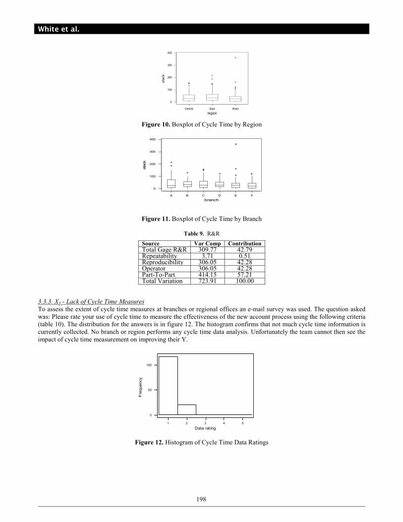
This X is somewhat self explanatory. With many branches and employees, the processing of new accounts can follow many different internal paths. The basic requirements are given in Operations Policy No 2140, but there is no process map included in this policy and each branch may adopt a different process and use different forms to collect needed new account information in line with the policy. It was impossible to measure the influence of a standard process directly as there really is no standard process. The team collected cycle time data across 6 different branches in 2 regions to see if perhaps a particular branch has a better standard new account practice (shorter cycle time). A boxplot was created to see if there were cycle time differences between branches or regions (figure 10). Looking at the results of the box plots it appears that no region or branch has a lock on a better performing process. The process appears to be equally ineffective in all of the locations and regions that were examined. Figure 11 illustrates a boxplot by branch. 3.3.2. X2 – Lack of Standard New Account Scoring.

This variable, like X1, is a symptom of lack of a standard process. The team found no one branch or region that claimed to have a standard scoring method. Team members claimed that many non-credit-worthy applications make it deep into the process using resources that could otherwise be used on good applications. Historically 25% of all new accounts submitted are rejected and usually at the regional level. To address the differences in new account scoring an R&R study was run by sending 15 fictitious new account applications to two branch new account officers and two regional credit officers. The results appear in table 9 and it is easy to see that the total R&R has a contribution of 42.79% (0.51% due to repeatability and 42.28% due to reproducibility). This means that there is a lot variation between an operator and others.

White et al.

198

WestEastCentral

400

300

200

100

0

region

stack

Figure 10. Boxplot of Cycle Time by Region

FEDCBA

400

300

200

100

0

branch

stack

Figure 11. Boxplot of Cycle Time by Branch

Table 9. R&R

3.3.3. X3 - Lack of Cycle Time Measures

To assess the extent of cycle time measures at branches or regional offices an e-mail survey was used. The question asked was: Please rate your use of cycle time to measure the effectiveness of the new account process using the following criteria (table 10). The distribution for the answers is in figure 12. The histogram confirms that not much cycle time information is currently collected. No branch or region performs any cycle time data analysis. Unfortunately the team cannot then see the impact of cycle time measurement on improving their Y.

54321

100

50

0

Data rating

Frequency

Figure 12. Histogram of Cycle Time Data Ratings

Source Var Comp Contribution Total Gage R&R 309.77 42.79 Repeatability 3.71 0.51 Reproducibility 306.05 42.28 Operator 306.05 42.28 Part-To-Part 414.15 57.21 Total Variation 723.91 100.00


199

Table 10. Criteria for Cycle Time Data Ratings

1 Do not collect any cycle time data. 2 Sometimes collect overall cycle time

information. 3 Cycle time data is sometimes collected at

the top process level 4 Cycle time data is collected at the top

process level and analyzed for improvement opportunities.

5 Cycle time data is collected at the step level and analyzed for improvement opportunities.

3.3.4. X4 – Transit Times

This X appeared in many process steps. There was no data at the process step level to tell us how much time applications and new account documents spent in transit. The preferred method for moving applications and new account documents between the customer, the branch and the region is the overnight mail pouch. As shown in the process icon there are also some alternate methods for transferring documents. Four basic methods were identified: Interoffice mail pouch, USPS, FEDEX and UPS. To gain some insight into the cycle time of this step, two team members agreed to track new accounts between them over a one- month time period. A cover sheet was put in front of each new account package. The new account officers were to record the date and time a step was finished and the package was ready for mailing and the date and time the package was opened for further processing. All transport process steps were included. As suspected, with a median of over 3 days, the transport steps do contribute to the overall cycle time. With 8 - 12 transport steps in the overall process the contribution to the overall cycle time would be about 24 days, close to 50% of our overall 49 days. Technology like FAX, E mail and the internet has yet to creep into this process. Looking further at this sample data we wanted to see if the transport step or mailing method were contributors. The descriptive statistics (figure 13 and the boxplots (figures 14 and 15) are as follows:

121086420


4.83.82.81.8


Variable: Cycle Time

2.0380

2.4389

3.0262

Maximum3rd QuartileMedian1st QuartileMinimum

NKurtosisSkewnessVarianceStDevMean

P-Value:A-Squared:

3.9421

3.6383

4.6857

12.6812 5.8089 3.0024 1.6561 0.1743

500.8866661.186478.524702.919713.85596

0.0002.011


95% Confidence Interval for Sigma


Anderson-Darling Normality Test

1211983

10

5

0

Transport Step

Cycle Time

Figure 13. Descriptive Statistics for Transport Times

Figure 14. Boxplot of Cycle Time by Transport Step

USPSUPSPouchFEDEX

10

5

0

Method

Cycle Tim

e

Figure 15. Boxplot of Cycle Time by Method

The boxplots show no major differences in step, although step 12 may have a bigger variance. Method appears to have some impact on the transport cycle time. As expected those processed using overnight mailing services (FEDEX and UPS)

White et al.

200

have shorter transport times than USPS or pouch methods, but these faster methods are not frequently used. This is consistent with the bank policy to use the mail pouch whenever possible. From the detailed process map using the above cycle time data, the sum of all transport steps was compared to the sum of all other process steps. The team found that 54% of the total time is in transport, leaving only 46% for other activities. Although this analysis is not completely accurate, as not all transactions pass through all steps, it does help confirm that transportation does contribute a great deal to the overall cycle time. 3.3.5. X5 – Incomplete Applications

Having to return either applications or documents to the customer will add cycle time with a rework loop. These loops are shown on the process map and highlighted with red return arrows. Using the information from X4 above each return loop will tend to add at least 3 days to the overall process. The team originally had no data on the defect rate. The team requested that 3 branches collect data on either returned applications or returned new account documents to see the extent of the problem. The results indicate that only 67% are error free, 33% of applications are returned and 10% consist of new documents. It appears that the application process and, to a lesser extent, the document completion process could use some improvement.

3.4 Hypothesis Test Every variable was tested to determine its impact. The next paragraphs illustrate that analysis. 3.4.1. X1 – Lack of Standard Process

Graphical boxplots failed to show a region or branch with a better process than any other. For completeness the team checked for equal variances using branch and region as the variables. Figure 16 (by branch) and figure 17 illustrate the tests for homogeneity. The null and alternate hypotheses are:

Ho: Variances across branches are equal. Ha: Variance of at least one branch is different than the rest.

Ho: Variances across regions are equal. Ha: Variance of at least on region is different than the rest.

1009080706050403020

95% Confidence Intervals for Sigmas

P-Value : 0.415

Test Statistic: 1.007

Levene's Test

P-Value : 0.000


Bartlett's Test

Factor Levels

F

E

D

C

B

A

30 35 40 45 50 55 60 65

95% Confidence Intervals for Sigmas

Bartlett's Test


P-Value : 0.078

Levene's Test


P-Value : 0.852

Factor Levels

Central

East

West

Figure 16. Test for Equal Variance by Branch Figure 17. Test for Equal Variance by Region

Since the data are not normal, the Levene’s test statistic is used. Since p>0.05 one cannot reject the null hypothesis and conclude that the variances are the same. To check for equality amongst medians a pair of Kruskal -Wallis Tests were used. The results are illustrated in figures 18 and 19.

Ho: Medians across branches are equal. Ha: Median of at least one branch is different than the rest.

Ho: Medians across regions are equal. Ha: Median of at least on region is different than the rest.

Kruskal-Wallis Test: stack versus region Region N Median Ave Rank Z Central 63 29.11 107.8 0.52 East 75 32.98 109.8 0.96 West 70 25.85 95.8 -1.48 Overall 208 104.5 H = 2.23 DF = 2 P = 0.328

Kruskal-Wallis Test: stack versus branch branch N Median Ave Rank Z A 50 27.29 108.3 0.51 B 25 33.02 112.9 0.75 C 35 31.52 106.7 0.24 D 28 27.93 109.1 0.43 E 33 28.39 102.2 -0.24 F 37 20.04 90.1 -1.60 Overall 208 104.5 H = 3.05 DF = 5 P = 0.692

Figure 18. Median Tests for Across Branches Figure 19. Median Tests for Across Regions Since p>0.05 for both tests the team concludes that the median cycle time of branches and regions are the same. Again this only leads us to believe that the process is broken throughout banks and there is no best practice to copy.


201

3.4.2. X2 – Lack of Standard New account Scoring

To further look at the differences in scoring between branches and regions we wanted to check the following hypothesis:

Ho: Mean new account scores are equal at branches and regional offices. Ha: Mean new account scores are not equal.

First new account scores were checked to insure normality. All data was found to be normally distributed. Next each operator in our mini gage study was checked for equal variances. The results indicate that the variance is the same. As suspected from the results of the gage study, there is a difference between operators in scoring new accounts. The regional new account officers scored new accounts about 30 points lower than the branches. The inconsistency in measures will have to be addressed in our solution. 3.4.3. X3 – Lack of Cycle Time Measures

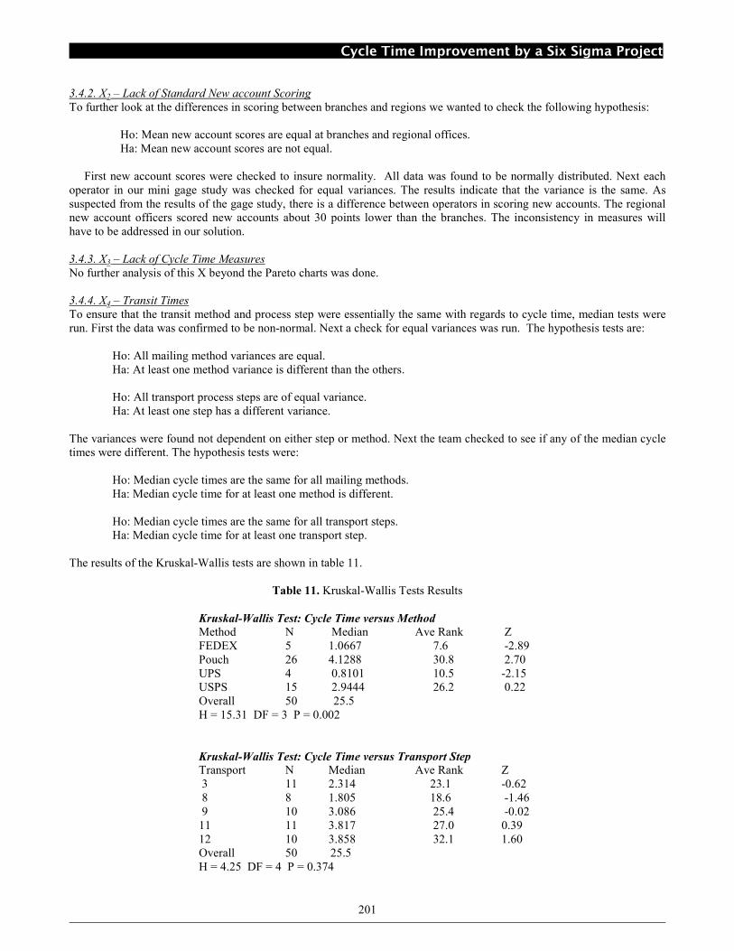
No further analysis of this X beyond the Pareto charts was done. 3.4.4. X4 – Transit Times

To ensure that the transit method and process step were essentially the same with regards to cycle time, median tests were run. First the data was confirmed to be non-normal. Next a check for equal variances was run. The hypothesis tests are:

Ho: All mailing method variances are equal. Ha: At least one method variance is different than the others.

Ho: All transport process steps are of equal variance. Ha: At least one step has a different variance.

The variances were found not dependent on either step or method. Next the team checked to see if any of the median cycle times were different. The hypothesis tests were:

Ho: Median cycle times are the same for all mailing methods. Ha: Median cycle time for at least one method is different.

Ho: Median cycle times are the same for all transport steps. Ha: Median cycle time for at least one transport step.

The results of the Kruskal-Wallis tests are shown in table 11.

Table 11. Kruskal-Wallis Tests Results

Kruskal-Wallis Test: Cycle Time versus Method

Method N Median Ave Rank Z FEDEX 5 1.0667 7.6 -2.89 Pouch 26 4.1288 30.8 2.70 UPS 4 0.8101 10.5 -2.15 USPS 15 2.9444 26.2 0.22 Overall 50 25.5 H = 15.31 DF = 3 P = 0.002

Kruskal-Wallis Test: Cycle Time versus Transport Step

Transport N Median Ave Rank Z 3 11 2.314 23.1 -0.62 8 8 1.805 18.6 -1.46 9 10 3.086 25.4 -0.02 11 11 3.817 27.0 0.39 12 10 3.858 32.1 1.60 Overall 50 25.5 H = 4.25 DF = 4 P = 0.374

White et al.

202

With a p < 0.05 median cycle times are influenced by transport method. FEDEX and UPS had lower transport cycle times. There were however only 9 data points out of our 50 samples represented by overnight carriers. With a p values > 0.05 the median cycle times are not influenced by the transport step.

3.4.5. X5 – Incomplete Applications

There was no direct data on how much additional cycle time was added due to rework. Also the team found that the largest problem was with returned applications. Using the detailed process map and cycle time estimates, we can roughly compare cycle times with complete applications with those that had to be returned. Since we are interested in changes in cycle time on the order of 5 or so days, we used Minitab’s sample size calculator to determine the number of samples needed. For a delta of 5 and a standard deviation of 20 (taken from the capability study) the sample size was calculated (power = 0.9). Results indicate that we need about 170 samples of each to detect a 5 day difference if one exists. Using simple observation of the map, we estimate there is about a 10.5 day difference in cycle time between those applications that are returned to the customer and those that are not.

3.5 Improve 3.5.1. DOE planning and selection

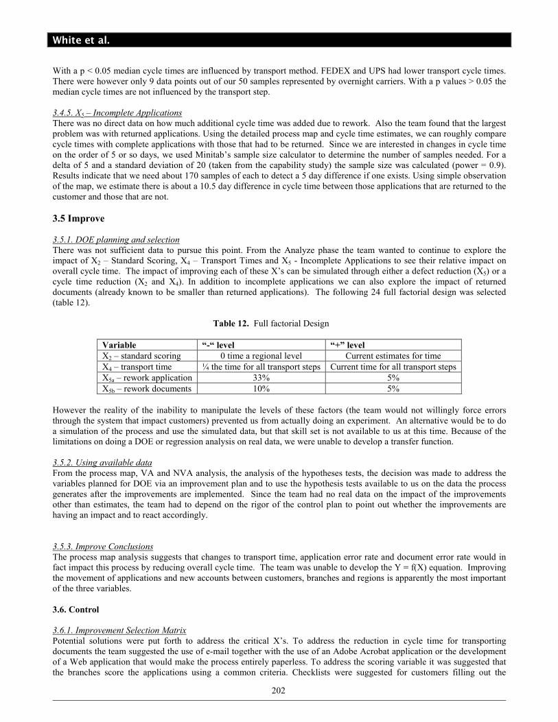
There was not sufficient data to pursue this point. From the Analyze phase the team wanted to continue to explore the impact of X2 – Standard Scoring, X4 – Transport Times and X5 - Incomplete Applications to see their relative impact on overall cycle time. The impact of improving each of these X’s can be simulated through either a defect reduction (X5) or a cycle time reduction (X2 and X4). In addition to incomplete applications we can also explore the impact of returned documents (already known to be smaller than returned applications). The following 24 full factorial design was selected (table 12).

Table 12. Full factorial Design

Variable “-“ level “+” level

X2 – standard scoring 0 time a regional level Current estimates for time

X4 – transport time ¼ the time for all transport steps Current time for all transport steps

X5a – rework application 33% 5%

X5b – rework documents 10% 5%

However the reality of the inability to manipulate the levels of these factors (the team would not willingly force errors through the system that impact customers) prevented us from actually doing an experiment. An alternative would be to do a simulation of the process and use the simulated data, but that skill set is not available to us at this time. Because of the limitations on doing a DOE or regression analysis on real data, we were unable to develop a transfer function.

3.5.2. Using available data

From the process map, VA and NVA analysis, the analysis of the hypotheses tests, the decision was made to address the variables planned for DOE via an improvement plan and to use the hypothesis tests available to us on the data the process generates after the improvements are implemented. Since the team had no real data on the impact of the improvements other than estimates, the team had to depend on the rigor of the control plan to point out whether the improvements are having an impact and to react accordingly. 3.5.3. Improve Conclusions

The process map analysis suggests that changes to transport time, application error rate and document error rate would in fact impact this process by reducing overall cycle time. The team was unable to develop the Y = f(X) equation. Improving the movement of applications and new accounts between customers, branches and regions is apparently the most important of the three variables.

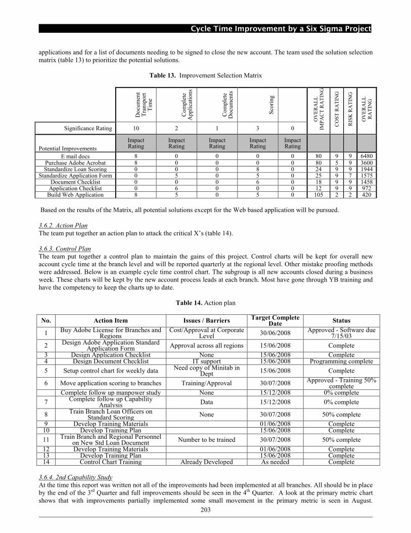
3.6. Control 3.6.1. Improvement Selection Matrix

Potential solutions were put forth to address the critical X’s. To address the reduction in cycle time for transporting documents the team suggested the use of e-mail together with the use of an Adobe Acrobat application or the development of a Web application that would make the process entirely paperless. To address the scoring variable it was suggested that the branches score the applications using a common criteria. Checklists were suggested for customers filling out the


203

applications and for a list of documents needing to be signed to close the new account. The team used the solution selection matrix (table 13) to prioritize the potential solutions.

Table 13. Improvement Selection Matrix

Do

cum

ent

Tra

nsp

ort

T

ime

Co

mp

lete

A

pp

lica

tion

s

Co

mp

lete

D

ocu

men

ts

Sco

ring

OV

ER

AL

L

IMP

AC

T R

AT

ING

CO

ST

RA

TIN

G

RIS

K R

AT

ING

OV

ER

AL

L

RA

TIN

G

Significance Rating 10 2 1 3 0

Potential Improvements

Impact Rating

Impact Rating

Impact Rating

Impact Rating

Impact Rating

E mail docs 8 0 0 0 0 80 9 9 6480 Purchase Adobe Acrobat 8 0 0 0 0 80 5 9 3600 Standardize Loan Scoring 0 0 0 8 0 24 9 9 1944

Standardize Application Form 0 5 0 5 0 25 9 7 1575 Document Checklist 0 0 0 6 0 18 9 9 1458

Application Checklist 0 6 0 0 0 12 9 9 972 Build Web Application 8 5 0 5 0 105 2 2 420

Based on the results of the Matrix, all potential solutions except for the Web based application will be pursued.

3.6.2. Action Plan

The team put together an action plan to attack the critical X’s (table 14). 3.6.3. Control Plan

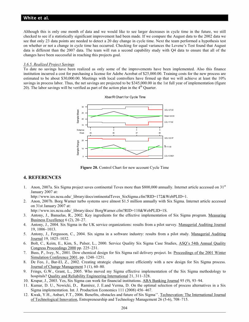
The team put together a control plan to maintain the gains of this project. Control charts will be kept for overall new account cycle time at the branch level and will be reported quarterly at the regional level. Other mistake proofing methods were addressed. Below is an example cycle time control chart. The subgroup is all new accounts closed during a business week. These charts will be kept by the new account process leads at each branch. Most have gone through YB training and have the competency to keep the charts up to date.

Table 14. Action plan

3.6.4. 2nd Capability Study

At the time this report was written not all of the improvements had been implemented at all branches. All should be in place by the end of the 3rd Quarter and full improvements should be seen in the 4th Quarter. A look at the primary metric chart shows that with improvements partially implemented some small movement in the primary metric is seen in August.

No. Action Item Issues / Barriers Target Complete Date

Status

1 Buy Adobe License for Branches and Regions

Cost/Approval at Corporate Level 30/06/2008 Approved - Software due

7/15/03

2 Design Adobe Application Standard Application Form Approval across all regions 15/06/2008 Complete

3 Design Application Checklist None 15/06/2008 Complete 4 Design Document Checklist IT support 15/06/2008 Programming complete

5 Setup control chart for weekly data Need copy of Minitab in Dept 15/06/2008 Complete

6 Move application scoring to branches Training/Approval 30/07/2008 Approved - Training 50% complete

Complete follow up manpower study None 15/12/2008 0% complete

7 Complete follow up Capability Analysis Data 15/12/2008 0% complete

8 Train Branch Loan Officers on Standard Scoring None 30/07/2008 50% complete

9 Develop Training Materials 01/06/2008 Complete 10 Develop Training Plan 15/06/2008 Complete

11 Train Branch and Regional Personnel on New Std Loan Document Number to be trained 30/07/2008 50% complete

12 Develop Training Materials 01/06/2008 Complete 13 Develop Training Plan 15/06/2008 Complete 14 Control Chart Training Already Developed As needed Complete

White et al.

204

Although this is only one month of data and we would like to see larger decreases in cycle time in the future, we still checked to see if a statistically significant improvement had been made. If we compare the August data to the 2002 data we see that only 23 data points are needed to detect a 20 day change in cycle time. Next the team performed a hypothesis test on whether or not a change in cycle time has occurred. Checking for equal variances the Levene’s Test found that August data is different than the 2007 data. The team will run a second capability study with Q4 data to ensure that all of the changes have been successful in reaching this projects goal. 3.6.5. Realized Project Savings

To date no savings have been realized as only some of the improvements have been implemented. Also this finance institution incurred a cost for purchasing a license for Adobe Acrobat of $25,000.00. Training costs for the new process are estimated to be about $30,000.00. Meetings with local controllers have firmed up that we will achieve at least the 10% savings in process labor. Thus, the net savings are projected to be $345,000.00 in the 1st full year of implementation (figure 20). The labor savings will be verified as part of the action plan in the 4th Quarter.

1Subgroup 2 3 4

15

20

25

30

Sample Mean

45 46 47 48Week

Mean=22.63

UCL=27.63

LCL=17.62

0

10

20

Sample Range

R=11.93

UCL=22.97

LCL=0.9021

Xbar/R Chart for Cycle Time

Figure 20. Control Chart for new account Cycle Time

4. REFERENCES

1. Anon, 2007a. Six Sigma project saves continental Teves more than $800,000 annually. Internet article accessed on 31st January 2007 at: http://www.ies.ncsu.edu/_library/docs/ontinentalTeves_SixSigma.cfm?RID=172&WebPLID=1.

2. Anon, 2007b. Borg Warner turbo systems save almost $1.5 million annually with Six Sigma. Internet article accessed on 31st January 2007 at: http://www.ies.ncsu.edu/_library/docs/ BorgWarner.cfm?RID=110&WebPLID=1S.

3. Antony, J., Banuelas, R., 2002. Key ingredients for the effective implementation of Six Sigma program. Measuring Business Excellence 6 (2), 20–27.

4. Antony, J., 2004. Six Sigma in the UK service organizations: results from a pilot survey. Managerial Auditing Journal 19, 1006–1013.

5. Antony, J., Fergusson, C., 2004. Six sigma in a software industry: results from a pilot study. Managerial Auditing Journal 19, 1025–1032.

6. Bolt, C., Keim, E., Kim, S., Palser, L., 2000. Service Quality Six Sigma Case Studies, ASQ’s 54th Annual Quality Congress Proceedings 2000 pp. 225–231.

7. Buss, P., Ivey, N., 2001. Dow chemical design for Six Sigma rail delivery project. In: Proceedings of the 2001 Winter Simulation Conference 2001, pp. 1248–1251.

8. De Feo, J., Bar-El, Z., 2002. Creating strategic change more efficiently with a new design for Six Sigma process. Journal of Change Management 3 (1), 60–80.

9. Frings, G.W., Grant, L., 2005. Who moved my Sigma effective implementation of the Six Sigma methodology to hospitals? Quality and Reliability Engineering International 21, 311–328.

10. Krupar, J., 2003. Yes, Six Sigma can work for financial institutions. ABA Banking Journal 95 (9), 93–94. 11. Kumar, D. U., Nowicki, D., Ramírez, J. E.and Verma, D. On the optimal selection of process alternatives in a Six

Sigma implementation. Int. J. Production Economics 111 (2008) 456–467. 12. Kwak, Y.H., Anbari, F.T., 2006. Benefits, obstacles and future of Six Sigma’’. Technovation: The International Journal

of Technological Innovation, Entrepreneurship and Technology Management 26 (5-6), 708–715.


205

13. McClusky, R., 2000. The rise, fall and revival of Six Sigma. Measuring Business Excellence 4 (2), 6–17. 14. Moorman, D.W., 2005. On the quest for Six Sigma. The American Journal of Surgery 189, 253–258. 15. Roberts, C.M., 2004. Six sigma signals. Credit Union Magazine 70 (1), 40–43. 16. Weiner, M., 2004. Six Sigma Communication World 21 (1), 26–29.

BIOGRAPHICAL SKETCH

Marcela White is a graduate Industrial Engineering from Autonomous University of Ciudad Juarez. She has the Green Belt Certification. Her areas of specialty include Total Quality Management and Supply Chain Management. He has more than twelve years experience in the maquiladora industry in Juarez region. Actually she works for a company in medical industry sector in Phoenix Arizona in logistic department.

Jorge Luis Garcia Alcaraz is a Professor at the Autonomous University of Ciudad Juarez. He has Bachelor and Masters Science Degree in Industrial Engineering from Colima Institute of Technology and also has a Doctorate Science Degree in Industrial Engineering from Ciudad Juarez Institute of Technology. His areas of specialty include multiattribute and multicriteria decision making, applied statistics, experimental optimization, design of experiments and mathematical programming. He is author and coauthor of several national and international journal publications.

Jesus Andres Hernandez Gomez is a Professor at the Autonomous University of Ciudad Juarez and Head of the Industrial Engineering Program at the same university. He has a Bachelor Degree in Industrial Engineering fron Autonomous University of Ciudad Juarez and a Master Degree in Business Administration and Specialty in TQM from Autonomous University of Chihuahua. His areas of specialty include quality improvement, statistical quality control and production management. He has more than ten years experience in the automotive industry.

Jorge Meza Jimenez he is professor at Colima Institute of Technology. He has a Bachelor Degree in Mechanical Industrial Engineer from Ciudad Guzman Institute of Technology, a Master Science Degree in Industrial Engineering from Aguascalientes Institute of Technology and a Doctorate Degree in Engineering of manufacturing Process from CIDESI (Engineering Center and industrial development at Queretaro). His line research is related to manufacturing processes and technological innovation.