DAG-Calculus: A Calculus for Parallel

ComputationUmut Acar

Carnegie Mellon University

Filip Sieczkowski

Inria

Gallium Seminar February 2016

Inria & LRI Université Paris Sud, CNRS

ArthurCharguéraud

MikeRainey

Inria

Parallel Computation

• Crucial for efficiency in the age of multicores

• Many different modes of use and language constructs

• Stress generally on efficiency, semantics not as well understood

function fib (n) if n <= 1 then n else let (x,y) = forkjoin (fib (n-1), fib (n-2)) in x + y

Fibonacci with fork-join

1. Perform two recursive calls in parallel2. Evaluate the

result

function fib (n) if n <= 1 then n else let (x,y) = (ref 0, ref 0) in finish { async (x := fib (n-1)); async (y := fib (n-2)) }; !x + !y

Fibonacci with async-finish

1. Perform two recursive calls in parallel

2. Synchronise on completion of parallel calls3. Read results of calls

and compute final result

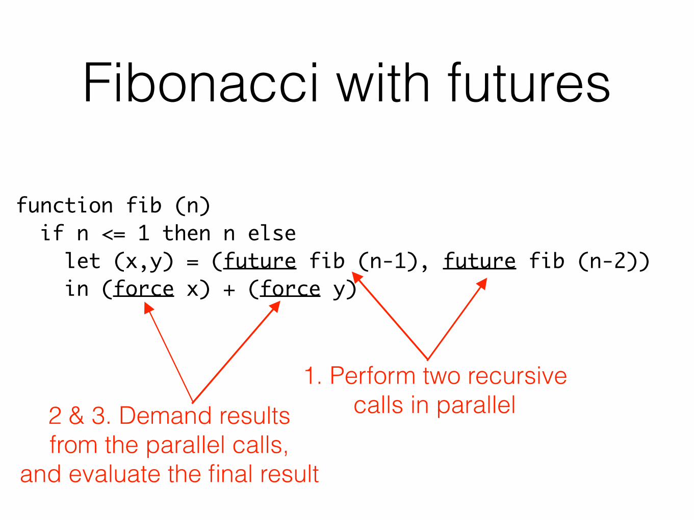
Fibonacci with futures

function fib (n) if n <= 1 then n else let (x,y) = (future fib (n-1), future fib (n-2)) in (force x) + (force y)

1. Perform two recursive calls in parallel2 & 3. Demand results

from the parallel calls, and evaluate the final result

Motivating questions

Is there a unifying model or calculus that can be used to express and study different forms of

parallelism?

Can such a calculus be realised efficiently in practice as a programming language, which can

serve, for example, as a target for compiling different forms of parallelism?

Parallelism patterns: fork-join, async-finish

fib(n)

K[ ]

fib(n-1) fib(n-2)

Parallelism patterns: futures

fib(n)

K[force(x)]

fib(n-1) fib(n-2)x y

K’[force(y)]

fib(n-1) fib(n-2)x y

Core idea — reify the dependency edges

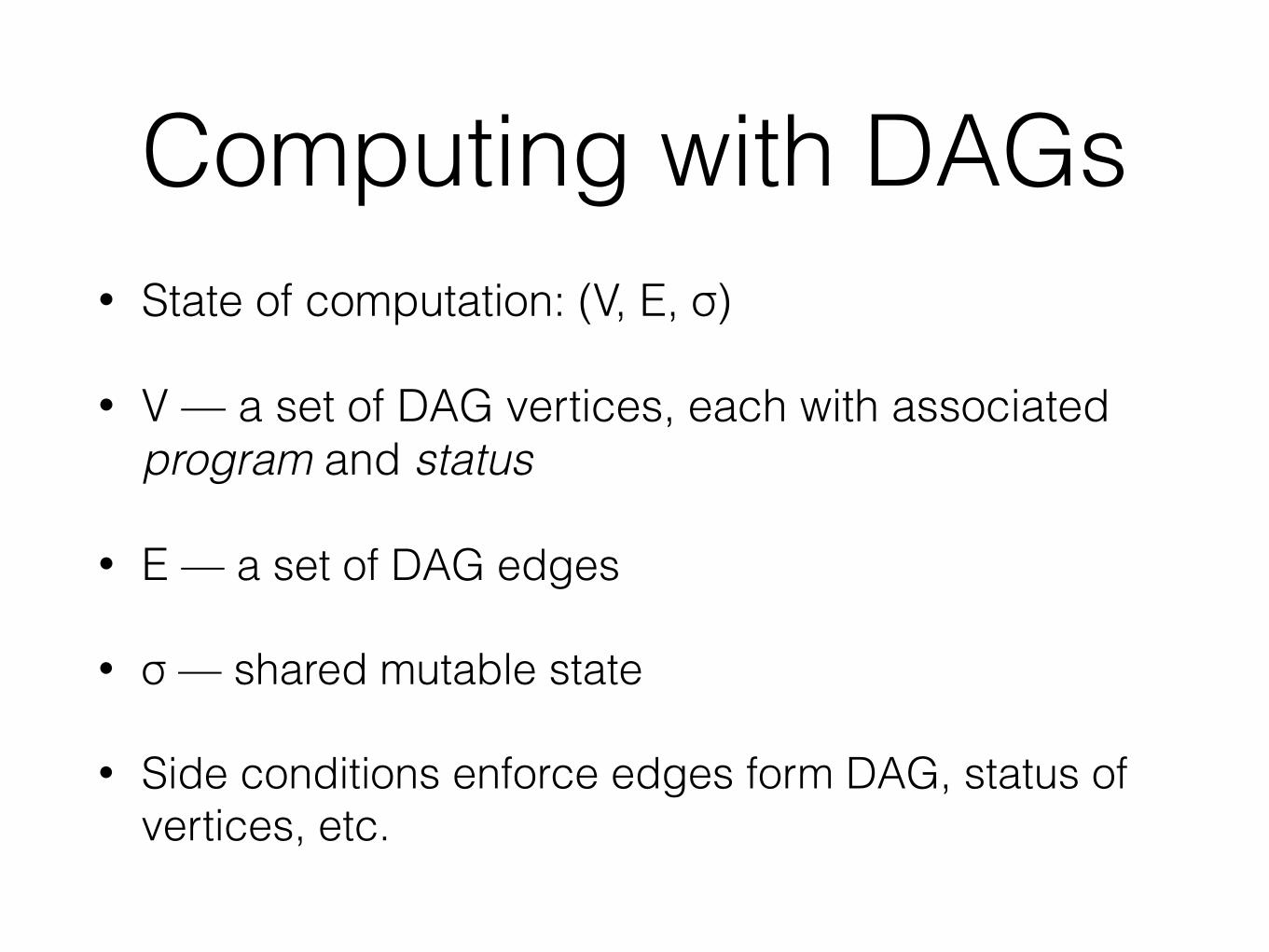
Computing with DAGs• State of computation: (V, E, σ)

• V — a set of DAG vertices, each with associated program and status

• E — a set of DAG edges

• σ — shared mutable state

• Side conditions enforce edges form DAG, status of vertices, etc.

Manipulating the DAG• Four commands that are used to dynamically modify the

computation DAG

• newTd(e) creates a new vertex in the DAG

• newEdge(e, e’) creates an edge from e to e’

• release(e) is called to mark that the vertex e is now set up and can be scheduled

• transfer(e) is a parallel control operator that transfers the outgoing edges of calling thread to e

The life-cycle of a vertex• Vertex can have one of four status values: New,

Released, eXecuting or Finished (N, R, X, F)

• Node created by running newTd has status N

• After calling release, its status is changed to R

• At this point it can be scheduled for execution, which sets the status to X

• After the execution terminates, the status is set to F

Operational Semantics (1)

�, fst (v1, v2)! v1,�Fst

�, snd (v1, v2)! v2,�Snd

l < dom(�)

�, alloc! l,�[l 7! ( )]Alloc

�(l) = v

�, ! l! v,�Deref

l 2 dom(�)

�, (l := v)! ( ),�[l 7! v]Assign

�, ((fun f x is e end) v)! e[ f 7! fun f x is e end][x 7! v],�Apply

k = fun f x is abort (K[x]) end

�,K[capture e]! e k,�Capture

�,K[abort e]! e,�Abort

�, e! e0,�0 8K0, e00. e < {K0[capture e00],K0[abort e00]}�,K[e]! K[e0],�0

Context

V(t) = (e,R) {t0 | (t0, t) 2 E} = ;V, E,�⇣ V[t 7! (e,X)], E,�

StartV(t) = (e1,X) �1, e1 ! e2,�2

V, E,�1 ⇣ V[t 7! (e2,X)], E,�2Step

V(t) = (v,X) E0 = E \ {(t, t0) | t0 2 dom(V)}V, E,�⇣ V[t 7! (( ),F)], E0,�

StopV(t) = (K[newTd e],X) t0 fresh

V, E,�⇣ V[t 7! (K[t0],X)][t0 7! (e,N)], E,�NewTd

V(t) = (K[release t0],X)V(t0) = (e,N)

V, E,�⇣ V[t 7! (K[( )],X)][t0 7! (e,R)], E,�Release

V(t) = (K[newEdge t1 t2],X) t1, t2 2 dom(V)status(V(t2)) 2 {N,R} E0 cycle-free

E0 = E ] (if status(V(t1)) = F then ; else {(t1, t2)})V, E,�⇣ V[t 7! (K[( )],X)], E0,�

NewEdge

V(t) = (K[transfer t0],X) status(V(t0)) = N {t00 | (t0, t00) 2 E} = ;E0 = E \ {(t, t00) | t00 2 dom(V)} ] {(t0, t00) | (t, t00) 2 E} E0 cycle-free

V, E,�⇣ V[t 7! (K[( )],X)], E0,�Transfer

Figure 2. Dynamic semantics for �DC . Recall that thread status are: N (new), R (released), X (executing) and F (finished).Besides, we write “status(V(t))” to denote the status of thread t, i.e. the second component of V(t).

The rule NewTd creates a new thread identified as t0,associates with it the expression e and the status N (new),and returns t0. The rule Release changes the status of thethread specified, namely t0, from N (new) to R (released).

The rule NewEdge adds a dependency edge betweentwo given threads, called t1 and t2. It is the programmer’sresponsibility to not introduce cyclic dependencies, otherwisethe program will be stuck. Furthermore, we restrict theaddition of an edge by requiring that the target vertex t2has not already started executing. Typically, the programmerwould only request the addition of edges when it can bededuced from the invariants of the program that the targetvertex has at least one incoming edge, and that this edgecannot be concurrently removed. Besides, note that the vertext1 at the source of the edge might already have completed itsexecution when newEdge is called. In this case, the operationis simply a no-op, in the sense that no edge is being added tothe DAG.

The rule Transfer describes the migration of the set ofoutgoing edges associated with the currently-running thread,called t, to another given thread, called t0. This operationis only permitted when t0 has status N (new) and has nooutgoing edges. These two restrictions are driven by ouruse of transfer in practice, and they allow for e�cientimplementation of this operation, in particular avoiding theneed to merge sets of outgoing edges.

The rule Capture and Abort describe the standard se-mantics of these control operators. The capture operator wasintroduced by Felleisen and Friedman [15] (where it is writ-ten C). It reifies the sequential evaluation context as a first-class value, and passes it to its argument. Formally, by ruleCapture, an expression of a form K[capture e] for somecontext K reduces to the application e k, where k denotesthe first-call reification of the context. The continuation k isdefined as �x. abort (K[x]), which involves the abort oper-ator, used to drop the context in which the abort expressionevaluates. More precisely, during the evaluation of e k, wemay eventually reach an expression of the form K0[k v]. Thisexpression beta-reduces to K0[abort (K[v])], which, by ruleAbort, evaluates to K[v]. This transition thus restores theoriginal context K, in which capture was called, pluggingin the value v to which the continuation k was applied.

4. Parallelism in the DAG Calculus

In this section, we show how to translate three classic, high-level parallel constructs into our DAG calculus.

4.1 Fork Join

To describe the translation of fork-join into the DAG calculus,we consider as source language a pure lambda-calculusextended with a fork-join construct, written e1 k e2 . In thisconstruct, also called parallel pair, reduction can take placeon either the left or the right branch. We present the language

DAG-Calculus: A Calculus for Parallel Computation 4 2015/11/20

�, fst (v1, v2)! v1,�Fst

�, snd (v1, v2)! v2,�Snd

l < dom(�)

�, alloc! l,�[l 7! ( )]Alloc

�(l) = v

�, ! l! v,�Deref

l 2 dom(�)

�, (l := v)! ( ),�[l 7! v]Assign

�, ((fun f x is e end) v)! e[ f 7! fun f x is e end][x 7! v],�Apply

k = fun f x is abort (K[x]) end

�,K[capture e]! e k,�Capture

�,K[abort e]! e,�Abort

�, e! e0,�0 8K0, e00. e < {K0[capture e00],K0[abort e00]}�,K[e]! K[e0],�0

Context

V(t) = (e,R) {t0 | (t0, t) 2 E} = ;V, E,�⇣ V[t 7! (e,X)], E,�

StartV(t) = (e1,X) �1, e1 ! e2,�2

V, E,�1 ⇣ V[t 7! (e2,X)], E,�2Step

V(t) = (v,X) E0 = E \ {(t, t0) | t0 2 dom(V)}V, E,�⇣ V[t 7! (( ),F)], E0,�

StopV(t) = (K[newTd e],X) t0 fresh

V, E,�⇣ V[t 7! (K[t0],X)][t0 7! (e,N)], E,�NewTd

V(t) = (K[release t0],X)V(t0) = (e,N)

V, E,�⇣ V[t 7! (K[( )],X)][t0 7! (e,R)], E,�Release

V(t) = (K[newEdge t1 t2],X) t1, t2 2 dom(V)status(V(t2)) 2 {N,R} E0 cycle-free

E0 = E ] (if status(V(t1)) = F then ; else {(t1, t2)})V, E,�⇣ V[t 7! (K[( )],X)], E0,�

NewEdge

V(t) = (K[transfer t0],X) status(V(t0)) = N {t00 | (t0, t00) 2 E} = ;E0 = E \ {(t, t00) | t00 2 dom(V)} ] {(t0, t00) | (t, t00) 2 E} E0 cycle-free

V, E,�⇣ V[t 7! (K[( )],X)], E0,�Transfer

Figure 2. Dynamic semantics for �DC . Recall that thread status are: N (new), R (released), X (executing) and F (finished).Besides, we write “status(V(t))” to denote the status of thread t, i.e. the second component of V(t).

The rule NewTd creates a new thread identified as t0,associates with it the expression e and the status N (new),and returns t0. The rule Release changes the status of thethread specified, namely t0, from N (new) to R (released).

The rule NewEdge adds a dependency edge betweentwo given threads, called t1 and t2. It is the programmer’sresponsibility to not introduce cyclic dependencies, otherwisethe program will be stuck. Furthermore, we restrict theaddition of an edge by requiring that the target vertex t2has not already started executing. Typically, the programmerwould only request the addition of edges when it can bededuced from the invariants of the program that the targetvertex has at least one incoming edge, and that this edgecannot be concurrently removed. Besides, note that the vertext1 at the source of the edge might already have completed itsexecution when newEdge is called. In this case, the operationis simply a no-op, in the sense that no edge is being added tothe DAG.

The rule Transfer describes the migration of the set ofoutgoing edges associated with the currently-running thread,called t, to another given thread, called t0. This operationis only permitted when t0 has status N (new) and has nooutgoing edges. These two restrictions are driven by ouruse of transfer in practice, and they allow for e�cientimplementation of this operation, in particular avoiding theneed to merge sets of outgoing edges.

The rule Capture and Abort describe the standard se-mantics of these control operators. The capture operator wasintroduced by Felleisen and Friedman [15] (where it is writ-ten C). It reifies the sequential evaluation context as a first-class value, and passes it to its argument. Formally, by ruleCapture, an expression of a form K[capture e] for somecontext K reduces to the application e k, where k denotesthe first-call reification of the context. The continuation k isdefined as �x. abort (K[x]), which involves the abort oper-ator, used to drop the context in which the abort expressionevaluates. More precisely, during the evaluation of e k, wemay eventually reach an expression of the form K0[k v]. Thisexpression beta-reduces to K0[abort (K[v])], which, by ruleAbort, evaluates to K[v]. This transition thus restores theoriginal context K, in which capture was called, pluggingin the value v to which the continuation k was applied.

4. Parallelism in the DAG Calculus

In this section, we show how to translate three classic, high-level parallel constructs into our DAG calculus.

4.1 Fork Join

To describe the translation of fork-join into the DAG calculus,we consider as source language a pure lambda-calculusextended with a fork-join construct, written e1 k e2 . In thisconstruct, also called parallel pair, reduction can take placeon either the left or the right branch. We present the language

DAG-Calculus: A Calculus for Parallel Computation 4 2015/11/20

�, fst (v1, v2)! v1,�Fst

�, snd (v1, v2)! v2,�Snd

l < dom(�)

�, alloc! l,�[l 7! ( )]Alloc

�(l) = v

�, ! l! v,�Deref

l 2 dom(�)

�, (l := v)! ( ),�[l 7! v]Assign

�, ((fun f x is e end) v)! e[ f 7! fun f x is e end][x 7! v],�Apply

k = fun f x is abort (K[x]) end

�,K[capture e]! e k,�Capture

�,K[abort e]! e,�Abort

�, e! e0,�0 8K0, e00. e < {K0[capture e00],K0[abort e00]}�,K[e]! K[e0],�0

Context

V(t) = (e,R) {t0 | (t0, t) 2 E} = ;V, E,�⇣ V[t 7! (e,X)], E,�

StartV(t) = (e1,X) �1, e1 ! e2,�2

V, E,�1 ⇣ V[t 7! (e2,X)], E,�2Step

V(t) = (v,X) E0 = E \ {(t, t0) | t0 2 dom(V)}V, E,�⇣ V[t 7! (( ),F)], E0,�

StopV(t) = (K[newTd e],X) t0 fresh

V, E,�⇣ V[t 7! (K[t0],X)][t0 7! (e,N)], E,�NewTd

V(t) = (K[release t0],X)V(t0) = (e,N)

V, E,�⇣ V[t 7! (K[( )],X)][t0 7! (e,R)], E,�Release

V(t) = (K[newEdge t1 t2],X) t1, t2 2 dom(V)status(V(t2)) 2 {N,R} E0 cycle-free

E0 = E ] (if status(V(t1)) = F then ; else {(t1, t2)})V, E,�⇣ V[t 7! (K[( )],X)], E0,�

NewEdge

V(t) = (K[transfer t0],X) status(V(t0)) = N {t00 | (t0, t00) 2 E} = ;E0 = E \ {(t, t00) | t00 2 dom(V)} ] {(t0, t00) | (t, t00) 2 E} E0 cycle-free

V, E,�⇣ V[t 7! (K[( )],X)], E0,�Transfer

Figure 2. Dynamic semantics for �DC . Recall that thread status are: N (new), R (released), X (executing) and F (finished).Besides, we write “status(V(t))” to denote the status of thread t, i.e. the second component of V(t).

The rule NewTd creates a new thread identified as t0,associates with it the expression e and the status N (new),and returns t0. The rule Release changes the status of thethread specified, namely t0, from N (new) to R (released).

The rule NewEdge adds a dependency edge betweentwo given threads, called t1 and t2. It is the programmer’sresponsibility to not introduce cyclic dependencies, otherwisethe program will be stuck. Furthermore, we restrict theaddition of an edge by requiring that the target vertex t2has not already started executing. Typically, the programmerwould only request the addition of edges when it can bededuced from the invariants of the program that the targetvertex has at least one incoming edge, and that this edgecannot be concurrently removed. Besides, note that the vertext1 at the source of the edge might already have completed itsexecution when newEdge is called. In this case, the operationis simply a no-op, in the sense that no edge is being added tothe DAG.

The rule Transfer describes the migration of the set ofoutgoing edges associated with the currently-running thread,called t, to another given thread, called t0. This operationis only permitted when t0 has status N (new) and has nooutgoing edges. These two restrictions are driven by ouruse of transfer in practice, and they allow for e�cientimplementation of this operation, in particular avoiding theneed to merge sets of outgoing edges.

The rule Capture and Abort describe the standard se-mantics of these control operators. The capture operator wasintroduced by Felleisen and Friedman [15] (where it is writ-ten C). It reifies the sequential evaluation context as a first-class value, and passes it to its argument. Formally, by ruleCapture, an expression of a form K[capture e] for somecontext K reduces to the application e k, where k denotesthe first-call reification of the context. The continuation k isdefined as �x. abort (K[x]), which involves the abort oper-ator, used to drop the context in which the abort expressionevaluates. More precisely, during the evaluation of e k, wemay eventually reach an expression of the form K0[k v]. Thisexpression beta-reduces to K0[abort (K[v])], which, by ruleAbort, evaluates to K[v]. This transition thus restores theoriginal context K, in which capture was called, pluggingin the value v to which the continuation k was applied.

4. Parallelism in the DAG Calculus

In this section, we show how to translate three classic, high-level parallel constructs into our DAG calculus.

4.1 Fork Join

To describe the translation of fork-join into the DAG calculus,we consider as source language a pure lambda-calculusextended with a fork-join construct, written e1 k e2 . In thisconstruct, also called parallel pair, reduction can take placeon either the left or the right branch. We present the language

DAG-Calculus: A Calculus for Parallel Computation 4 2015/11/20

�, fst (v1, v2)! v1,�Fst

�, snd (v1, v2)! v2,�Snd

l < dom(�)

�, alloc! l,�[l 7! ( )]Alloc

�(l) = v

�, ! l! v,�Deref

l 2 dom(�)

�, (l := v)! ( ),�[l 7! v]Assign

�, ((fun f x is e end) v)! e[ f 7! fun f x is e end][x 7! v],�Apply

k = fun f x is abort (K[x]) end

�,K[capture e]! e k,�Capture

�,K[abort e]! e,�Abort

�, e! e0,�0 8K0, e00. e < {K0[capture e00],K0[abort e00]}�,K[e]! K[e0],�0

Context

V(t) = (e,R) {t0 | (t0, t) 2 E} = ;V, E,�⇣ V[t 7! (e,X)], E,�

StartV(t) = (e1,X) �1, e1 ! e2,�2

V, E,�1 ⇣ V[t 7! (e2,X)], E,�2Step

V(t) = (v,X) E0 = E \ {(t, t0) | t0 2 dom(V)}V, E,�⇣ V[t 7! (( ),F)], E0,�

StopV(t) = (K[newTd e],X) t0 fresh

V, E,�⇣ V[t 7! (K[t0],X)][t0 7! (e,N)], E,�NewTd

V(t) = (K[release t0],X)V(t0) = (e,N)

V, E,�⇣ V[t 7! (K[( )],X)][t0 7! (e,R)], E,�Release

V(t) = (K[newEdge t1 t2],X) t1, t2 2 dom(V)status(V(t2)) 2 {N,R} E0 cycle-free

E0 = E ] (if status(V(t1)) = F then ; else {(t1, t2)})V, E,�⇣ V[t 7! (K[( )],X)], E0,�

NewEdge

V(t) = (K[transfer t0],X) status(V(t0)) = N {t00 | (t0, t00) 2 E} = ;E0 = E \ {(t, t00) | t00 2 dom(V)} ] {(t0, t00) | (t, t00) 2 E} E0 cycle-free

V, E,�⇣ V[t 7! (K[( )],X)], E0,�Transfer

Figure 2. Dynamic semantics for �DC . Recall that thread status are: N (new), R (released), X (executing) and F (finished).Besides, we write “status(V(t))” to denote the status of thread t, i.e. the second component of V(t).

The rule NewTd creates a new thread identified as t0,associates with it the expression e and the status N (new),and returns t0. The rule Release changes the status of thethread specified, namely t0, from N (new) to R (released).

The rule NewEdge adds a dependency edge betweentwo given threads, called t1 and t2. It is the programmer’sresponsibility to not introduce cyclic dependencies, otherwisethe program will be stuck. Furthermore, we restrict theaddition of an edge by requiring that the target vertex t2has not already started executing. Typically, the programmerwould only request the addition of edges when it can bededuced from the invariants of the program that the targetvertex has at least one incoming edge, and that this edgecannot be concurrently removed. Besides, note that the vertext1 at the source of the edge might already have completed itsexecution when newEdge is called. In this case, the operationis simply a no-op, in the sense that no edge is being added tothe DAG.

The rule Transfer describes the migration of the set ofoutgoing edges associated with the currently-running thread,called t, to another given thread, called t0. This operationis only permitted when t0 has status N (new) and has nooutgoing edges. These two restrictions are driven by ouruse of transfer in practice, and they allow for e�cientimplementation of this operation, in particular avoiding theneed to merge sets of outgoing edges.

The rule Capture and Abort describe the standard se-mantics of these control operators. The capture operator wasintroduced by Felleisen and Friedman [15] (where it is writ-ten C). It reifies the sequential evaluation context as a first-class value, and passes it to its argument. Formally, by ruleCapture, an expression of a form K[capture e] for somecontext K reduces to the application e k, where k denotesthe first-call reification of the context. The continuation k isdefined as �x. abort (K[x]), which involves the abort oper-ator, used to drop the context in which the abort expressionevaluates. More precisely, during the evaluation of e k, wemay eventually reach an expression of the form K0[k v]. Thisexpression beta-reduces to K0[abort (K[v])], which, by ruleAbort, evaluates to K[v]. This transition thus restores theoriginal context K, in which capture was called, pluggingin the value v to which the continuation k was applied.

4. Parallelism in the DAG Calculus

In this section, we show how to translate three classic, high-level parallel constructs into our DAG calculus.

4.1 Fork Join

To describe the translation of fork-join into the DAG calculus,we consider as source language a pure lambda-calculusextended with a fork-join construct, written e1 k e2 . In thisconstruct, also called parallel pair, reduction can take placeon either the left or the right branch. We present the language

DAG-Calculus: A Calculus for Parallel Computation 4 2015/11/20

�, fst (v1, v2)! v1,�Fst

�, snd (v1, v2)! v2,�Snd

l < dom(�)

�, alloc! l,�[l 7! ( )]Alloc

�(l) = v

�, ! l! v,�Deref

l 2 dom(�)

�, (l := v)! ( ),�[l 7! v]Assign

�, ((fun f x is e end) v)! e[ f 7! fun f x is e end][x 7! v],�Apply

k = fun f x is abort (K[x]) end

�,K[capture e]! e k,�Capture

�,K[abort e]! e,�Abort

�, e! e0,�0 8K0, e00. e < {K0[capture e00],K0[abort e00]}�,K[e]! K[e0],�0

Context

V(t) = (e,R) {t0 | (t0, t) 2 E} = ;V, E,�⇣ V[t 7! (e,X)], E,�

StartV(t) = (e1,X) �1, e1 ! e2,�2

V, E,�1 ⇣ V[t 7! (e2,X)], E,�2Step

V(t) = (v,X) E0 = E \ {(t, t0) | t0 2 dom(V)}V, E,�⇣ V[t 7! (( ),F)], E0,�

StopV(t) = (K[newTd e],X) t0 fresh

V, E,�⇣ V[t 7! (K[t0],X)][t0 7! (e,N)], E,�NewTd

V(t) = (K[release t0],X)V(t0) = (e,N)

V, E,�⇣ V[t 7! (K[( )],X)][t0 7! (e,R)], E,�Release

V(t) = (K[newEdge t1 t2],X) t1, t2 2 dom(V)status(V(t2)) 2 {N,R} E0 cycle-free

E0 = E ] (if status(V(t1)) = F then ; else {(t1, t2)})V, E,�⇣ V[t 7! (K[( )],X)], E0,�

NewEdge

V(t) = (K[transfer t0],X) status(V(t0)) = N {t00 | (t0, t00) 2 E} = ;E0 = E \ {(t, t00) | t00 2 dom(V)} ] {(t0, t00) | (t, t00) 2 E} E0 cycle-free

V, E,�⇣ V[t 7! (K[( )],X)], E0,�Transfer

Figure 2. Dynamic semantics for �DC . Recall that thread status are: N (new), R (released), X (executing) and F (finished).Besides, we write “status(V(t))” to denote the status of thread t, i.e. the second component of V(t).

The rule NewTd creates a new thread identified as t0,associates with it the expression e and the status N (new),and returns t0. The rule Release changes the status of thethread specified, namely t0, from N (new) to R (released).

The rule NewEdge adds a dependency edge betweentwo given threads, called t1 and t2. It is the programmer’sresponsibility to not introduce cyclic dependencies, otherwisethe program will be stuck. Furthermore, we restrict theaddition of an edge by requiring that the target vertex t2has not already started executing. Typically, the programmerwould only request the addition of edges when it can bededuced from the invariants of the program that the targetvertex has at least one incoming edge, and that this edgecannot be concurrently removed. Besides, note that the vertext1 at the source of the edge might already have completed itsexecution when newEdge is called. In this case, the operationis simply a no-op, in the sense that no edge is being added tothe DAG.

The rule Transfer describes the migration of the set ofoutgoing edges associated with the currently-running thread,called t, to another given thread, called t0. This operationis only permitted when t0 has status N (new) and has nooutgoing edges. These two restrictions are driven by ouruse of transfer in practice, and they allow for e�cientimplementation of this operation, in particular avoiding theneed to merge sets of outgoing edges.

The rule Capture and Abort describe the standard se-mantics of these control operators. The capture operator wasintroduced by Felleisen and Friedman [15] (where it is writ-ten C). It reifies the sequential evaluation context as a first-class value, and passes it to its argument. Formally, by ruleCapture, an expression of a form K[capture e] for somecontext K reduces to the application e k, where k denotesthe first-call reification of the context. The continuation k isdefined as �x. abort (K[x]), which involves the abort oper-ator, used to drop the context in which the abort expressionevaluates. More precisely, during the evaluation of e k, wemay eventually reach an expression of the form K0[k v]. Thisexpression beta-reduces to K0[abort (K[v])], which, by ruleAbort, evaluates to K[v]. This transition thus restores theoriginal context K, in which capture was called, pluggingin the value v to which the continuation k was applied.

4. Parallelism in the DAG Calculus

In this section, we show how to translate three classic, high-level parallel constructs into our DAG calculus.

4.1 Fork Join

To describe the translation of fork-join into the DAG calculus,we consider as source language a pure lambda-calculusextended with a fork-join construct, written e1 k e2 . In thisconstruct, also called parallel pair, reduction can take placeon either the left or the right branch. We present the language

DAG-Calculus: A Calculus for Parallel Computation 4 2015/11/20

Operational Semantics (2)

�, fst (v1, v2)! v1,�Fst

�, snd (v1, v2)! v2,�Snd

l < dom(�)

�, alloc! l,�[l 7! ( )]Alloc

�(l) = v

�, ! l! v,�Deref

l 2 dom(�)

�, (l := v)! ( ),�[l 7! v]Assign

�, ((fun f x is e end) v)! e[ f 7! fun f x is e end][x 7! v],�Apply

k = fun f x is abort (K[x]) end

�,K[capture e]! e k,�Capture

�,K[abort e]! e,�Abort

�, e! e0,�0 8K0, e00. e < {K0[capture e00],K0[abort e00]}�,K[e]! K[e0],�0

Context

V(t) = (e,R) {t0 | (t0, t) 2 E} = ;V, E,�⇣ V[t 7! (e,X)], E,�

StartV(t) = (e1,X) �1, e1 ! e2,�2

V, E,�1 ⇣ V[t 7! (e2,X)], E,�2Step

V(t) = (v,X) E0 = E \ {(t, t0) | t0 2 dom(V)}V, E,�⇣ V[t 7! (( ),F)], E0,�

StopV(t) = (K[newTd e],X) t0 fresh

V, E,�⇣ V[t 7! (K[t0],X)][t0 7! (e,N)], E,�NewTd

V(t) = (K[release t0],X)V(t0) = (e,N)

V, E,�⇣ V[t 7! (K[( )],X)][t0 7! (e,R)], E,�Release

V(t) = (K[newEdge t1 t2],X) t1, t2 2 dom(V)status(V(t2)) 2 {N,R} E0 cycle-free

E0 = E ] (if status(V(t1)) = F then ; else {(t1, t2)})V, E,�⇣ V[t 7! (K[( )],X)], E0,�

NewEdge

V(t) = (K[transfer t0],X) status(V(t0)) = N {t00 | (t0, t00) 2 E} = ;E0 = E \ {(t, t00) | t00 2 dom(V)} ] {(t0, t00) | (t, t00) 2 E} E0 cycle-free

V, E,�⇣ V[t 7! (K[( )],X)], E0,�Transfer

Figure 2. Dynamic semantics for �DC . Recall that thread status are: N (new), R (released), X (executing) and F (finished).Besides, we write “status(V(t))” to denote the status of thread t, i.e. the second component of V(t).

The rule NewTd creates a new thread identified as t0,associates with it the expression e and the status N (new),and returns t0. The rule Release changes the status of thethread specified, namely t0, from N (new) to R (released).

The rule NewEdge adds a dependency edge betweentwo given threads, called t1 and t2. It is the programmer’sresponsibility to not introduce cyclic dependencies, otherwisethe program will be stuck. Furthermore, we restrict theaddition of an edge by requiring that the target vertex t2has not already started executing. Typically, the programmerwould only request the addition of edges when it can bededuced from the invariants of the program that the targetvertex has at least one incoming edge, and that this edgecannot be concurrently removed. Besides, note that the vertext1 at the source of the edge might already have completed itsexecution when newEdge is called. In this case, the operationis simply a no-op, in the sense that no edge is being added tothe DAG.

The rule Transfer describes the migration of the set ofoutgoing edges associated with the currently-running thread,called t, to another given thread, called t0. This operationis only permitted when t0 has status N (new) and has nooutgoing edges. These two restrictions are driven by ouruse of transfer in practice, and they allow for e�cientimplementation of this operation, in particular avoiding theneed to merge sets of outgoing edges.

The rule Capture and Abort describe the standard se-mantics of these control operators. The capture operator wasintroduced by Felleisen and Friedman [15] (where it is writ-ten C). It reifies the sequential evaluation context as a first-class value, and passes it to its argument. Formally, by ruleCapture, an expression of a form K[capture e] for somecontext K reduces to the application e k, where k denotesthe first-call reification of the context. The continuation k isdefined as �x. abort (K[x]), which involves the abort oper-ator, used to drop the context in which the abort expressionevaluates. More precisely, during the evaluation of e k, wemay eventually reach an expression of the form K0[k v]. Thisexpression beta-reduces to K0[abort (K[v])], which, by ruleAbort, evaluates to K[v]. This transition thus restores theoriginal context K, in which capture was called, pluggingin the value v to which the continuation k was applied.

4. Parallelism in the DAG Calculus

In this section, we show how to translate three classic, high-level parallel constructs into our DAG calculus.

4.1 Fork Join

To describe the translation of fork-join into the DAG calculus,we consider as source language a pure lambda-calculusextended with a fork-join construct, written e1 k e2 . In thisconstruct, also called parallel pair, reduction can take placeon either the left or the right branch. We present the language

DAG-Calculus: A Calculus for Parallel Computation 4 2015/11/20

�, fst (v1, v2)! v1,�Fst

�, snd (v1, v2)! v2,�Snd

l < dom(�)

�, alloc! l,�[l 7! ( )]Alloc

�(l) = v

�, ! l! v,�Deref

l 2 dom(�)

�, (l := v)! ( ),�[l 7! v]Assign

�, ((fun f x is e end) v)! e[ f 7! fun f x is e end][x 7! v],�Apply

k = fun f x is abort (K[x]) end

�,K[capture e]! e k,�Capture

�,K[abort e]! e,�Abort

�, e! e0,�0 8K0, e00. e < {K0[capture e00],K0[abort e00]}�,K[e]! K[e0],�0

Context

V(t) = (e,R) {t0 | (t0, t) 2 E} = ;V, E,�⇣ V[t 7! (e,X)], E,�

StartV(t) = (e1,X) �1, e1 ! e2,�2

V, E,�1 ⇣ V[t 7! (e2,X)], E,�2Step

V(t) = (v,X) E0 = E \ {(t, t0) | t0 2 dom(V)}V, E,�⇣ V[t 7! (( ),F)], E0,�

StopV(t) = (K[newTd e],X) t0 fresh

V, E,�⇣ V[t 7! (K[t0],X)][t0 7! (e,N)], E,�NewTd

V(t) = (K[release t0],X)V(t0) = (e,N)

V, E,�⇣ V[t 7! (K[( )],X)][t0 7! (e,R)], E,�Release

V(t) = (K[newEdge t1 t2],X) t1, t2 2 dom(V)status(V(t2)) 2 {N,R} E0 cycle-free

E0 = E ] (if status(V(t1)) = F then ; else {(t1, t2)})V, E,�⇣ V[t 7! (K[( )],X)], E0,�

NewEdge

V(t) = (K[transfer t0],X) status(V(t0)) = N {t00 | (t0, t00) 2 E} = ;E0 = E \ {(t, t00) | t00 2 dom(V)} ] {(t0, t00) | (t, t00) 2 E} E0 cycle-free

V, E,�⇣ V[t 7! (K[( )],X)], E0,�Transfer

Figure 2. Dynamic semantics for �DC . Recall that thread status are: N (new), R (released), X (executing) and F (finished).Besides, we write “status(V(t))” to denote the status of thread t, i.e. the second component of V(t).

The rule NewTd creates a new thread identified as t0,associates with it the expression e and the status N (new),and returns t0. The rule Release changes the status of thethread specified, namely t0, from N (new) to R (released).

The rule NewEdge adds a dependency edge betweentwo given threads, called t1 and t2. It is the programmer’sresponsibility to not introduce cyclic dependencies, otherwisethe program will be stuck. Furthermore, we restrict theaddition of an edge by requiring that the target vertex t2has not already started executing. Typically, the programmerwould only request the addition of edges when it can bededuced from the invariants of the program that the targetvertex has at least one incoming edge, and that this edgecannot be concurrently removed. Besides, note that the vertext1 at the source of the edge might already have completed itsexecution when newEdge is called. In this case, the operationis simply a no-op, in the sense that no edge is being added tothe DAG.

The rule Transfer describes the migration of the set ofoutgoing edges associated with the currently-running thread,called t, to another given thread, called t0. This operationis only permitted when t0 has status N (new) and has nooutgoing edges. These two restrictions are driven by ouruse of transfer in practice, and they allow for e�cientimplementation of this operation, in particular avoiding theneed to merge sets of outgoing edges.

The rule Capture and Abort describe the standard se-mantics of these control operators. The capture operator wasintroduced by Felleisen and Friedman [15] (where it is writ-ten C). It reifies the sequential evaluation context as a first-class value, and passes it to its argument. Formally, by ruleCapture, an expression of a form K[capture e] for somecontext K reduces to the application e k, where k denotesthe first-call reification of the context. The continuation k isdefined as �x. abort (K[x]), which involves the abort oper-ator, used to drop the context in which the abort expressionevaluates. More precisely, during the evaluation of e k, wemay eventually reach an expression of the form K0[k v]. Thisexpression beta-reduces to K0[abort (K[v])], which, by ruleAbort, evaluates to K[v]. This transition thus restores theoriginal context K, in which capture was called, pluggingin the value v to which the continuation k was applied.

4. Parallelism in the DAG Calculus

In this section, we show how to translate three classic, high-level parallel constructs into our DAG calculus.

4.1 Fork Join

To describe the translation of fork-join into the DAG calculus,we consider as source language a pure lambda-calculusextended with a fork-join construct, written e1 k e2 . In thisconstruct, also called parallel pair, reduction can take placeon either the left or the right branch. We present the language

DAG-Calculus: A Calculus for Parallel Computation 4 2015/11/20

Encoding fork-join〚forkjoin (e1, e2)〛=

capture (fn k =>let l1 = alloc l2 = alloc

t1 = newTd (l1 :=〚e1〛) t2 = newTd (l2 :=〚e2〛) t = newTd (k (!l1, !l2))

in newEdge(t1, t); newEdge(t2, t) transfer(t); release(t); release(t1); release(t2))

Encoding async-finish〚t | async(e)〛=

let t’ = newTd(〚t | e〛)in newEdge(t’, t); release(t’)

〚t | finish(e)〛= capture (fn k => let t2 = newTd(k ()) t1 = newTd(〚t2 | e〛) in newEdge(t1, t2); transfer(t2); release(t2); release(t1))

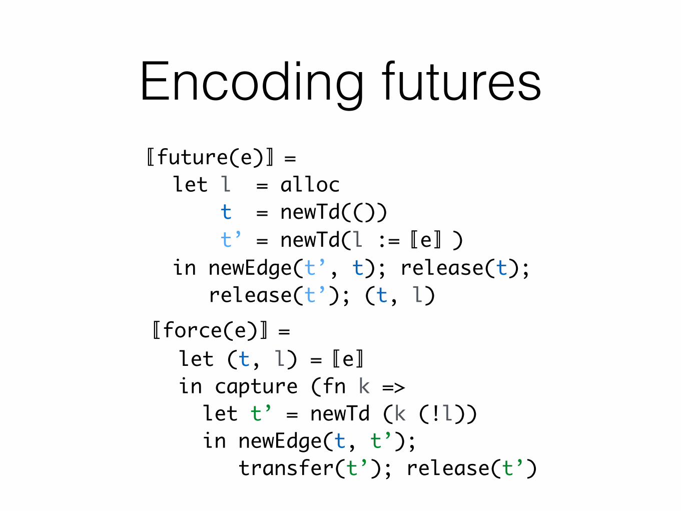
Encoding futures〚future(e)〛=

let l = alloc t = newTd(()) t’ = newTd(l :=〚e〛)in newEdge(t’, t); release(t); release(t’); (t, l)

〚force(e)〛= let (t, l) =〚e〛 in capture (fn k => let t’ = newTd (k (!l)) in newEdge(t, t’); transfer(t’); release(t’)

Proving the encodings correct: the technique

• Compiler-style proof of simulation

• Need backwards-simulation due to nondeterminism

• Problem: partially evaluated encodings do not correspond to any source terms

• Solution: an intermediate, annotated language,two-step proof

• Keep the structure and allow partial evaluation of parallel primitives

Also in the paper

• Scheduling DAG-calculus computations using work stealing

• Data-structures for efficient implementation of DAG edges

• Experimental evaluation of implementation

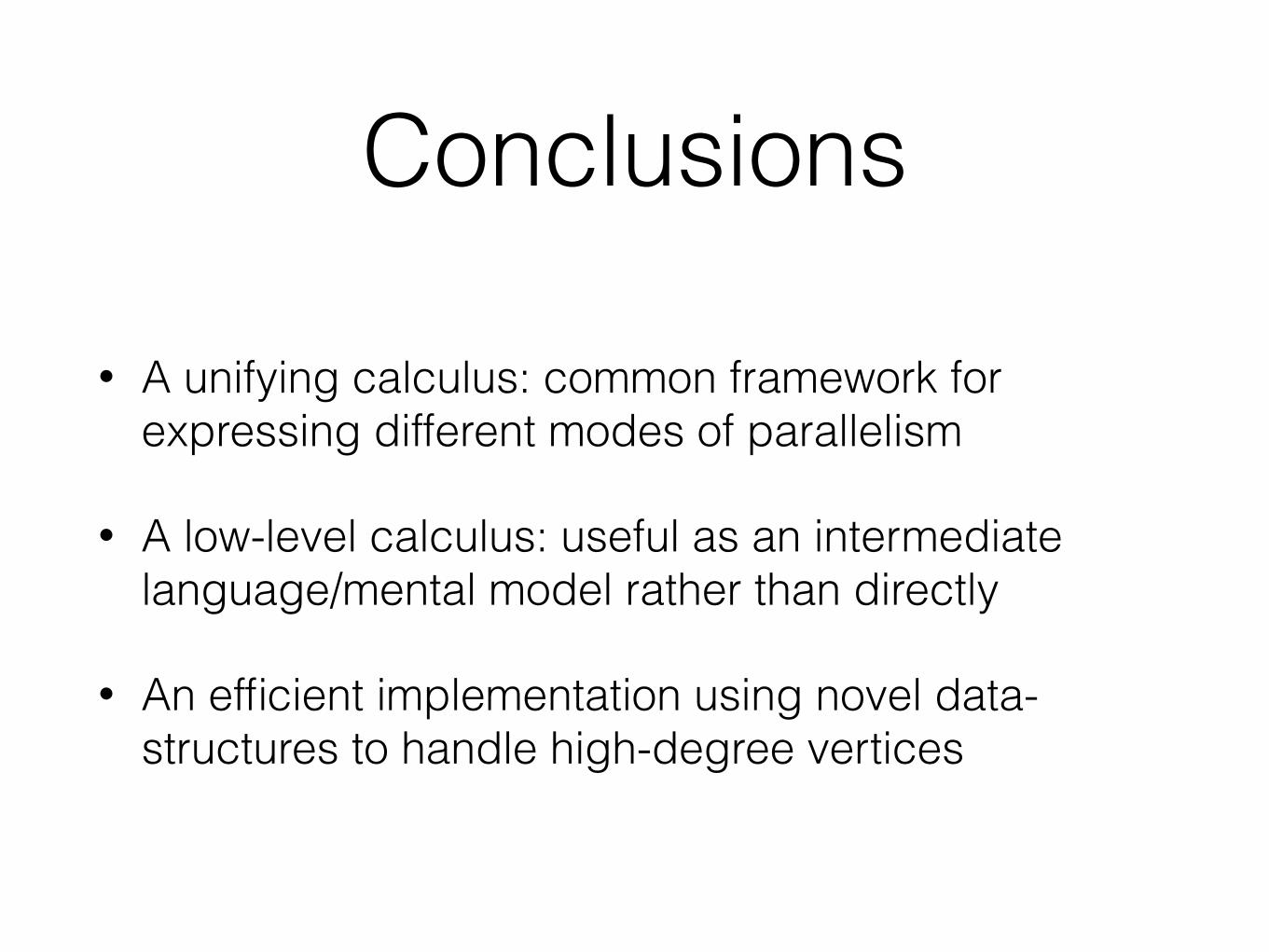
Conclusions

• A unifying calculus: common framework for expressing different modes of parallelism

• A low-level calculus: useful as an intermediate language/mental model rather than directly

• An efficient implementation using novel data-structures to handle high-degree vertices