Dalitz Plot Analysis of D Decays

Luigi Moroni

INFN-Milano

Dalitz Analysis of Heavy Flavor Decays

• Infinite power tool!– It provides a “complete observation” of the decay– Everything could be in principle measured

• from the dynamical features of the HF decay mechanism,– Relative importance of non-spector processes

• up to the CP-violating phases, mixing, etc– Just recall from Bo: probably the only clean way to get it

• We already learned a lot on charm

• But, as we know, – strong dynamic effects, if not properly accounted for,

would completely hide or at least confuse the underlying fundamental physics.

Outline

• In this talk I will address all the key issues of the HF Dalitz analysis– Formalization problems

– Failure of the traditional “isobar” model

– Need for the K-matrix approach

– Implications for the future Dalitz analyses in the B-sector

• Will discuss these issues in the context of the recent D++-+ Dalitz analysis we performed in FOCUS– A lot to be learned

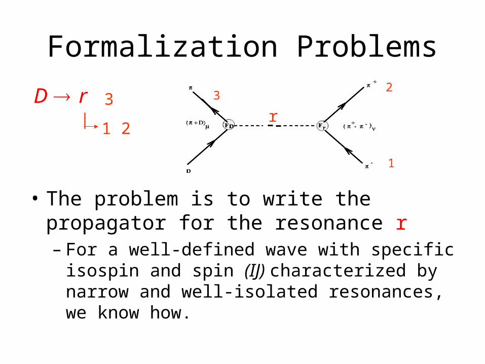
Formalization Problems

• The problem is to write the propagator for the resonance r– For a well-defined wave with specific isospin and

spin (IJ) characterized by narrow and well-isolated resonances, we know how.

rr3

1

2D r

|1 2

3

•the propagator is of the simple Breit-Wigner type

1 3 13 2 212

1(cos )

J Jr

D r Jr r r

A F F p p Pm m im

����������������������������

traditionalisobar modelj

j jj

Aia e M

Spin 0

Spin 1

Spin 2 )1cos3()(2

)2(

1

1322

13

13

ppP

ppP

P

J

J

J

21

21

)339(

)1(

1

4422

22

pRpRF

pRF

F

•the decay amplitude is

•the decay matrix element

when the specific IJ–wave is characterized by large and heavily overlapping resonances (just as the scalars!), the problem is not that simple.

1( )I iK

where K is the matrix for the scattering of particles 1 and 2.

In this case, it can be demonstrated on very general grounds that the propagator may be written in the context of the K-matrix approach as

Indeed, it is very easy to realize that the propagation is no longer dominated by a single resonance but is the result of a complicated interplay among resonances.

i.e., to write down the propagator we need to know the related scattering K-matrix

In contrast

What is K-matrix?

• It follows from S-matrix and because of S-matrix unitarity it is real

• Viceversa, any real K-matrix would generate an unitary S-matrix

• This is the real advantage of the K-matrix approach:– It drastically simplifies the formalization of any scattering

problem since the unitarity of S is automatically preserved

1/ 2 1/ 22S I i T 1 1K T i 1( )T I iK K

From Scattering to Production

• Thanks to I.J.R. Aitchison (Nucl. Phys. A189 (1972) 514), the K-matrix approach can be extended to production processes

• In technical language,

– From

– To

• The P-vector describes the coupling at the production with each channel involved in the process– In our case the production is the D decay

1( )T I iK K 1( )F I iK P

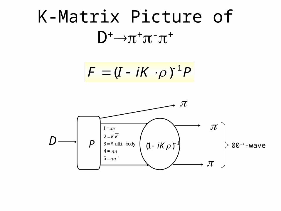
K-Matrix Picture of D++-+

D

P

1

2

3 Multi body

4 =

5 '

K K

1(1 )iK

1( )F I iK P

00++-wave

Failure of the Isobar Model

• At this point, on the basis of a pretty solid theory, it is very easy to understand when we can employ the traditional Isobar Model and when not.

• It turns out that– for a single pole problem, far away of any threshold, K-

matrix amplitude reduces to the standard BW formula.• The two descriptions are equivalent

– In all the other cases, the BW representation is not any more valid

• The most severe problem is that it does not respect unitarity

Add BW Add K

The Unitarity circle

Add BW

Add K

An Explicit Example

• Adding BWs ala “Isobar Model”– Breaks the Unitarity

– And heavily modify the phase motion!

21 0

20 0 0

1 / 2( )

( )(1 )jK A

k kj jA A

g s s s mF I iK f

m s s s s s s

The decay amplitude may be written, in general, as a coherent sumof BW terms for waves with well-isolated resonances plus K-matrix terms for waves with overlapping resonances.

00

1 1

( ) i i

m ni i iBW K

i i i ii i m

A D a e a e F a e F

Can safely say that in general K-matrix formalization is just required by scalars (J=0), whose general form is

KiF

Summarizing

Where can we get a reliable s-wave scattering parametrization from?

• In other words, we need to know K to proceed.• A global fit to all the available data has been performed!

* p0n,n, ’n, |t|0.2 (GeV/c2)GAMSGAMS

* pn, 0.30|t|1.0 (GeV/c2)GAMSGAMS

* BNLBNL

*p- KKn

CERN-MunichCERN-Munich

::

* Crystal BarrelCrystal Barrel

* Crystal BarrelCrystal Barrel

* Crystal BarrelCrystal Barrel

* Crystal BarrelCrystal Barrel

pp

pp , ,

pp K+K-, KsKs, K+s

np -, KsK-, KsKs-

-p0n, 0|t|1.5 (GeV/c2)E852E852*

At rest, from liquid 2H

At rest, from gaseous

At rest, from liquid

At rest, from liquid

2H

2D2H

“K-matrix analysis of the 00++-wave in the mass region below 1900 MeV’’ V.V Anisovich and A.V.Sarantsev Eur.Phys.J.A16 (2003) 229

( ) ( ) 200 0

20 0 0

1 2( )

( )(1 )

scatti j scatt A

ij ij scattA A

g g s s s mK s f

m s s s s s s

( )ig is the coupling constant of the bare state to the meson channel

scattijf

0s describe a smooth part of the K-matrix elements

20 0( 2) ( )(1 )A A As s m s s s suppresses the false kinematical singularity

at s = 0 near the threshold

and

is a 5x5 matrix (i,j=1,2,3,4,5)

'

IJijK

K K1= 2= 3=4 4= 5=

A&S

A&S K-matrix poles, couplings etc.

4 '

0.65100 0.24844 0.52523 0 0.38878 0.36397

1.20720 0.91779 0.55427 0 0.38705 0.29448

1.56122 0.37024 0.23591 0.62605 0.18409 0.18923

1.21257 0.34501 0.39642 0.97644 0.19746 0.00357

1.81746 0.15770 0.179

KKPoles g g g g g

0 11 12 13 14 15

0

15 0.90100 0.00931 0.20689

3.30564 0.26681 0.16583 0.19840 0.32808 0.31193

1.0 0.2

scatt scatt scatt scatt scatt scatt

A A

s f f f f f

s s

A&S T-matrix poles and couplings

4 '13.1 96.5 80.9 98.6 102.1

116.8 100.2 61.9 140

( , / 2)

(1.019, 0.038) 0.415 0.580 0.1482 0.484 0.401

(1.306, 0.167) 0.406 0.105 0.8912 0.142

KKi i i i i

i i i i

m g g g g g

e e e e e

e e e e

.0 133.0

97.8 97.4 91.1 115.5 152.4

151.5 149.6 123.3 170.6

0.225

(1.470, 0.960) 0.758 0.844 1.681 0.431 0.175

(1.489, 0.058) 0.246 0.134 0.4867 0.100 0

i

i i i i i

i i i i

e

e e e e e

e e e e

133.9

.6 126.7 101.1

.115

(1.749, 0.165) 0.536 0.072 0.160 0.313

i

i i i i i

e

e e e e e

A&S fit does not need a as measured in the isobar fit

FOCUS D s +

++- analysis

Observe:

•f0(980)

•f2(1270)

•f0(1500) Sideband

Signal

Yield Ds+ = 1475 50

S/N Ds+ = 3.41

PLB 585 (2004) 200

First fits to charm Dalitz plots in the K-matrix approach!

C.L fit 3 %

sD

Low mass projection High mass projection

+

+20 +

(S - wave)π 87.04 ± 5.60 ± 4.17 0(fixed)

f (1275)π 9.74 4.49 2.63 168.0 18.7 2.5

ρ (1450)π 6.56 ± 3.43 ± 3.31 234.9 ±19.5 ±13.3

decay channel phase (deg)fit fractions (%)

r

j

2iδ 2 2r r 12 13

r 2iδ 2 2j j 12 13j

a e A dm dmf =

a e A dm dm

Yield DYield D++ = 1527 = 1527 5151

S/N DS/N D++ = 3.64 = 3.64

FOCUS D+ ++- analysis

Sideband Signal

PLB 585 (2004) 200

2lowm

2highm

D

C.L fit 7.7 %

K-matrix fit results

Low mass projection High mass projection

18 11.7

+

+2

0 +

(S - wave)π 56.00 ± 3.24 ± 2.08 0(fixed)

f (1275)π 11.74 1.90 0.23 -47.5 .7

ρ (770)π 30.82 ± 3.14 ± 2.29 -139.4 ±16.5 ± 9.9

decay channel phase (deg)fit fractions (%)

No new ingredient (resonance) required not present in the scattering!

With

Without

C.L. ~ 7.5%

Isobar analysis of D+ ++would instead require a new scalar meson:

C.L. ~ 10-6

m = 442.6± 27.0 MeV/c = 340.4 ± 65.5 MeV/c preliminary

What about -meson then?

• Can conclude that – Do not need anything more than what is already in

the s-wave phase-shift to explain the main feature of D 3 Dalitz plot

• Or, if you prefer,– Any -like object in the D decay should be

consistent with the same -like object measured in the scattering.

• Just by a simple insertion of KK-1 in the decay amplitude F

• We can view the decay as consisting of an initial production of the five virtual states , KK,’and 4which then scatter via the physical T-matrix into the final state.

• The Q-vector contains the production amplitude of each virtual channel in the decay

1 1 1 1( ) ( )F I iK P I iK KK P TK P TQ

Even more: from P to Q-vector

Q-vector for Ds

• s-wave dominated by an initial production of and KK-bar states

The two peaks of the ratios correspond to the two dips of the normalizing modulus, while the two peaks due to the K-matrix singularities, visible in the normalization plot, cancel out in the ratios.

The normalizing modulus

Ratio of moduli of Q-vector amplitudes

Q-vector for D+

• The same!– s-wave dominated by an initial production of

and KK-bar states

The resulting picture

• The s-wave decay amplitude primarily arises from a ss-bar contribution– Cabibbo favored for Ds

– Cabibbo suppressed together with the competing dd-bar contribution for D+

• The measured fit fractions seems to confirm this picture– s-wave decay fraction, 87% for Ds and only 56% for D+

– The dd-bar contribution in D+ case evidently prefers to couple to a vector state like (770), that alone accounts for about 30% of the decay.

Conclusions• Dalitz plot analysis is and will be a crucial tool to extract physics

from the HF decays• Nevertheless, to fully exploit this unlimited potential a systematic

revision of the amplitude formalization is required• Thanks to FOCUS, K-matrix approach has been shown to be the

real breakthrough • Its application has been decisive in clearing up a situation which

recently became quite fuzzy and confusing– new “ad hoc” resonances were required to understand data, e.g. (600) and

(900)• Strong dynamics effects in D-decays now seem under control and

fully consistent with those measured by light-quark experiments• The new scenario is very promising for the future measurements of

the CP violating phases in the B sector, where a proper description of the different amplitudes is essential.