preliminary study of d0 k 0 decays with dalitz plots
TRANSCRIPT

Work supported by Department of Energy contract DE-AC02-76SF00515
Preliminary Study of D0 K 0 Decays with Dalitz Plots
Moira Gresham
ERULF
Reed College
Stanford Linear Accelerator Center
Menlo Park, CA
August 13, 2002
Prepared in partial fulfillment of the requirements of the Office of Science, DOE
Energy Research Undergraduate Laboratory Fellowship under the direction of Ray
Cowan in the MIT Lepton-Quark Studies group at SLAC.
SLAC-PUB-9401
SLAC, Stanford University, Stanford, CA 94309

Moira Gresham / DOE ERULF Research Paper 2002 2
Table of Contents
Abstract 3
Introduction 4
Methods and Materials 7
Results 12
Discussion and Conclusions 13
Acknowledgements 14
Tables and Figures 15
Appendix 22
Literature Cited 23

Moira Gresham / DOE ERULF Research Paper 2002 3
Abstract
Preliminary Study of D0 K 0 Decays with Dalitz Plots. MOIRA GRESHAM (Reed College, Portland, OR 97202) RAY COWAN (MIT Laboratory for Nuclear Science, Cambridge, MA 02139)
Particle physicists study the smallest particles and most basic rules of their
interactions in humankind’s current scope. The Charm Analysis Working Group (CWG) of the BaBar Collaboration studies decays involving the charm quark. They currently study mixing in D decays, an interesting and poorly understood phenomenon in current physics models. We, as part of the CWG, investigated the plausibility of using Dalitz plots and the BaBar analysis framework to study mixing in Wrong Sign (WS) D0 Kππ0 decays. Others in the CWG have studied mixing in the 2-body decay, D0 Kπ. The 3-body decay analyzed with the RooFitDalitz analysis package and Dalitz plots provides more information and another way of separating Doubly Cabibbo Suppressed Decays (DCSD) from mixing -- which share the same end products. Through doing many simulations, we have demonstrated the usefulness of this approach. We selected D0 Kππ0 events from Simulation Production run #4 (SP4) and BaBar’s run 1 and run 2. We made Dalitz plots with this data. Now that we better understand Dalitz plots and software, we plan to select WS D0 Kππ0 events and perform rate fits as discussed in BaBar Analysis Document (BAD) #443, as well as fits for several different decay times and resonances, in order to further distinguish DCSD from mixing.
Moira Gresham / DOE ERULF Research Paper 2002 4
Introduction
Fruitful scientific research happens on frontiers. Elementary particle physics
sits on the primordial frontier that separates us from nature’s deepest secrets. The
smallest, most fundamental particles found by humans are quarks (named up, down,
charm, strange, top, and bottom – u, d, c, s, t and b), leptons (electron, muon, tau, and
their associated neutrinos), and force-mediating particles (photon, gluon, Z, and W).
These particles and the accepted rules for their interactions form the Standard Model of
particle physics. Humans instinctively make models to explain nature. To better
understand nature, we must constantly push and test our models. The Standard Model of
particle physics is no exception! It is not in stasis, and not entirely convincing or well
understood. Interesting physics lurks.
We find quarks bound together as mesons (in groups of two) or baryons (in groups
of three). Mesons and baryons are classified as hadrons, particles that interact via the
strong force. Quarks carry properties such as spin (1/2), charge (± 1/3 or 2/3), and mass.
Their properties propagate; we observe their combined spin, charge, and mass in mesons
and baryons -- just as we observe the combined properties of baryons and leptons (for
example the proton, neutron, and electron in atoms) in larger bound groups. Two quarks
with equal and opposite charge compose a neutral meson. Neutral mesons have revealed
a fundamental asymmetry in our universe -- Charge-Parity (CP) violation. CP violation
may account for the abundance of matter (as opposed to anti-matter) in our universe; it is
one phenomenon that ‘allows’ us to exist. 0K / 0K , 0D / 0D , and 0B / 0B (the “ 0 ”
implies neutral; the bar implies antimatter) are the interesting neutral mesons that exhibit

Moira Gresham / DOE ERULF Research Paper 2002 5
mixing. The mixing phenomenon interests us on its own; in addition, through mixing we
observe CP violation and other interesting physics (Griffiths 1987, Perkins 2000).
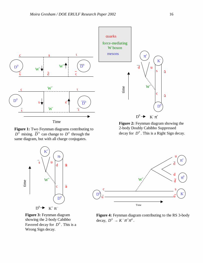
Particles decay. Following conservation laws, they spontaneously ‘break apart’
and recombine into other particles. Richard Feynman thought of a revealing way to
describe these processes using diagrams. Any given particle can decay in many different
ways, or channels; different Feynman diagrams describe the probability of each decay
channel. We should interpret the decay of any given particle as a combination of all
possible decay paths. Interestingly, there is a decay channel open to neutral mesons in
which, for example, 0K changes to 0K and vice versa. Consequently, we should view
neutral mesons as a linear combination -- a mix -- of 0M and 0M . (I use “M” for Meson,
in general.) We call this phenomenon mixing (See Fig. 1).
We may peek at interesting elementary mechanisms through the study of
mixing. 0D meson mixing is difficult to observe (compared to that of K and B mesons)
because it is predicted to be very small (Rmixing ~ 0-10-6 in the Standard Model) and
because D particles have a short lifetime compared with their mixing period Physicists
do not understand 0D mixing well; it "carries a large potential for discovery of new
physics" (Liu, 1995 p.2). Poorly determined parameters exist in the equations describing
0D mixing. Also, other kinds of 0D decays produce the same end products and further
inhibit our ability to measure 0D mixing.
0D decays can be categorized as right sign (RS) or wrong sign (WS). Right sign
decays occur most often. For example, the end products of a RS decay for the 0D – the
Cabibbo Favored (CF) decay -- are +−πK . (Written 0D → +−πK , where +, -, 0 are their
respective charges in units of one electron charge.) Likewise, the end products of a RS

Moira Gresham / DOE ERULF Research Paper 2002 6
0D decay are −+πK (see Fig. 2). The end products of a D0 WS, Doubly Cabibbo
Suppressed Decay (DCSD) are −+πK (see Fig. 3). This kind of WS decay is
approximately 400 times less likely. Inconveniently, DCSD decays produce the same
products as mixing. Because they have the same decay end-products, distinguishing
DCSD events from mixing events is challenging. When the goal is to study mixing,
DCSD events are considered primarily as "annoying ... background" (Liu, 1995, p.3).
Particle physicists have speculated about D mixing since the discovery of the
charm quark (Gaillard, 1975). In the first few years of 0D / 0D mixing studies, people
searched for −+→ πKD0 assuming mixing was the only contributor; this led to false
confidence in a mixing rate (Rmixing) due to the contribution of that "annoying" DCSD
background. Later, researchers moved to studying semileptonic (for example, D0 → K-
e+νe) decays, which are not subject to the DCSD background (Liu, 1995, p.3). However,
interest in 0D hadronic decays (i.e. 0D →hadrons) has recently reemerged (Liu,1995).
Since BaBar (the big particle detector at SLAC) has recorded many 0D decays in the last
several years, we have the capability to measure D mixing through hadronic decays with
enhanced sensitivity. With such a large data set, we can expect the mixing parameters to
show up in the interference term of the equation describing the 0D hadronic decay rate
(Liu,1995). See the appendix for rate equations.
We must know how a decay starts (i.e. was the original particle 0D or a 0D ?)
in order to determine whether DCSD or mixing occurred. Therefore, we ‘tag’ our events
using the decays D* +→D0π+ and D* -→ 0D π -. The ‘extra’ charged pion tells us
whether a particle started as 0D or 0D .

Moira Gresham / DOE ERULF Research Paper 2002 7
To extend the current BaBar mixing analysis using two-body,
±→ πmKDD )( 00 decays, we study mixing by analyzing 3-body hadronic decays
( 000 )( ππ ±→ mKDD ) (see Fig. 4). The third ‘body’ of the 0D decay allows for Dalitz
analysis. Dalitz analysis involves plotting the squared invariant mass (inv. mass2 =
Energy2 - momentum2) of the three particles, in combinations of two, in a two-
dimensional scatter plot (see Figs 5A & B). For example, in the decay, D→ABC, we
might plot MassAB2 versus MassBC
2. A Dalitz plot reveals the substructure of a decay. In
other words, if the density at a certain mass (say M, along the AB axis) is high, we say
that there was a resonance at M and the decay probably happened as D→MC, M→AB
(which ‘sums’ to D→ABC). We can make such a plot of an event for several different
times and see how the resonances change with time. We have enough knowledge of
possible resonances for mixing and DCSD to distinguish between the two types.
Remember that a particle decays through every possible mechanism, and the relative
densities for each resonance give the relative probabilities (Amplitude2) for different
decay mechanisms. Thus, we can measure amounts of mixing and DCSD with time
through time dependent Dalitz analysis. We venture out onto the primordial frontier of
elementary particles to test the Standard Model by studying poorly understood mixing
quantities.�
Materials and Methods
Dataset
Since elementary particles are very small -- and most ‘live’ for a very short period
of time (small fractions of a second) -- we have to use sophisticated, sensitive instruments
to produce and detect them. BaBar, which stands for B/Bbar, is one such instrument

Moira Gresham / DOE ERULF Research Paper 2002 8
(BaBar, B.Aubert et al., 2002). (B’s are mesons with b quarks, and are produced when
e+e-→ bb .) It is the detector "attached" to the PEPII rings at the end of the Stanford Linac
(linear accelerator). BaBar was designed, primarily, to detect B meson decays. The
energy at which positrons and electrons (coming from the PEP-II rings) collide is optimal
for the production of B mesons. BaBar and the PEP-II project was designed to catalog
and analyze many, many B decays in order to study CP (Charge-Parity) violation. In
addition, since the cc (the state that precedes D meson events) production cross-section is
just as large as that of bb , BaBar also has a large sample of D meson events. (Cross-
section relates to the probability with which an event occurs. Larger cross-section implies
higher probability.) The Charm Analysis Working Group (CWG) at BaBar analyzes these
D events to search for new and interesting physics.
High Energy physicists often use computer simulations -- also known as Monte
Carlos -- to better understand all of the complicated effects associated with extracting
unique physics numbers from complex particle detectors. A Monte Carlo simulation
‘knows’, in good detail, the geometry and other properties of the BaBar detector. In
Monte Carlo simulations, using random number generators and known physics models,
the computer generates events and passes them through the detector simulation. This
allows one to understand, with some confidence, how the detector and analysis programs
perform.
We use both simulated Monte Carlo data and ‘real’ BaBar/PEPII data. Our 40 fb-1
of simulated data comes from BaBar’s Simulation Production run #4 (SP4). SP4, created
in 2001, is the latest simulation available. We use Monte Carlo data from generic cc

Moira Gresham / DOE ERULF Research Paper 2002 9
modes. Our 57.1 fb-1 of ‘real’ BaBar/PEPII data comes from BaBar’s run 1 (2000) and
part of run 2 (before December, 2001).
Analysis Method
Dalitz Analysis Technique
We use a relatively new method for charm mixing analysis; we examine the
phases and amplitudes of resonances for our decay as a function of time in Dalitz plots.
Others in the CWG have studied hadronic D decays with Dalitz plots in search of mixing
-- but not D0→ Kππ0 decays. In general, a three-body decay can be characterized by two
variables (Perkins, 1987, p.130; Podolsky D. 1998). Given a decay, P→ABC, we
typically choose any two of the variables: mAB2, mBC
2, and mCA2 (where mij
2 = (pi + pj)
2,
the squared invariant mass of particles i and j) as the axes for our Dalitz plot. As
discussed below, this allows one to read the invariant mass of an intermediate resonance
directly from the plot. If only kinematics (that is, conservation of momentum and energy)
determines the decay of a parent particle, P, then a Dalitz plot, by construction, should
show a uniform distribution over the kinematically allowed region (Perkins, 132). In the
relativistic limit, this region resembles a triangle with rounded edges (see Fig. 6). One
can easily determine the upper, lower, right, and left asymptotes for such a plot using
conservation of energy. In the rest frame of the parent particle, the upper/right and
lower/left asymptotes (mijmax and mijmin, respectively) are: mijmax = mP – mk and mijmin
= mi + mj. (For an exact specification of kinematic boundaries in Dalitz plots, see
Jackson, 2000.) We are most interested in the dynamics of decays. If there exists
substructure in a decay (in other words, if a particle decays through intermediate
channels) we detect it in a Dalitz plot, since, in this case, the probability of finding an

Moira Gresham / DOE ERULF Research Paper 2002 10
event with a given mass distribution is not uniform across phase space. The substructure
of a decay is determined by intermediate resonances. Particle physicists care about the
relative probabilities of resonances – given by the Amplitude2 of the resonance.
Typically, Breit-Wigner distributions are used to describe resonances (Jackson, 1964). If
a resonance exists, it will show up on a Dalitz plot as a band of higher density centered
on1 the mass of the intermediate particle. The relative densities of bands correspond to
relative Amplitude2 (see Fig. 7). If intermediate particles have intrinsic spin, additional
angular momentum constraints exist for the corresponding resonance. This translates to
‘lobes’ in the resonance bands of Dalitz plots (see Fig. 8). For example, if a spin zero
parent particle decays through a spin-1 (say, AB) resonance to spin zero daughters, it is
very unlikely to find particle C moving perpendicular to A and B but very likely to find it
moving parallel or anti-parallel. This corresponds to a ‘hole’ near the middle of the
resonance band and a reinforcement at the ends; the density along the band varies like
cos2θ where θ is the angle between particle C and particle A (or B) in the parent’s center-
of-mass (CMS) frame. Since Breit-Wigners -- which describe particle resonances --
contain complex amplitudes and phases, different resonances can interfere and show up
as depleted or enhanced areas on the Dalitz plot. The Dalitz plot beautifully demonstrates
that, to fully describe these directly unobservable decay resonances, we must use
complex wave functions rather than probabilities (see Fig. 8). Importantly, looking at
Dalitz plots of a certain decay at several different decay times should show changes in
resonant contributions with time.
1 Actually, to be exact, the band is centered slightly below the mass. See the Jackson reference.

Moira Gresham / DOE ERULF Research Paper 2002 11
Specifically, we wish to examine the wrong sign (WS) 3-body decays,
00 ππ −+→ KD and 00 ππ +−→ KD (the charge conjugate). In these WS decays, DCSD
and mixing occur at different rates. Thus a change, with time, in 00 ππ −+→ KD (or
00 ππ +−→ KD ) substructure, as well as interference between mixing and DCSD, can
allow us to identify and study D mixing (Liu, T. 1995). However, before we study the
WS decays exclusively, we plan to include the much more abundant 00 ππ +−→ KD and
00 ππ −+→ KD RS decays in our dataset and fits in order to check that our analysis
technique works for 00 / DD 3-body decays in general.
Generate/Fit method – tools:
We plan to fit for the relative amplitudes and phases of resonances in the decay
mode of interest. To check that our fitting method is accurate, we will eventually
compare fits with real data to the fits with simulated data. We will use BaBar analysis
tools to accomplish this. RooFitDalitz is the new tool of interest.
� RooFitDalitz (RFD) is a package for doing Dalitz plot fits. It is based on the
RooFit toolkit, and also relies on EvtGen - a BaBar event generator package (Dvoretskii,
A. 2002). The RooFit packages provide a toolkit for modeling the expected distribution
of events in a physics analysis. Models can be used to perform likelihood fits, produce
plots, and generate "toy Monte Carlo" samples for various studies. The RooFit tools are
integrated with the object-oriented and interactive ROOT graphical environment (Kirkby,
2001). EvtGen (Ryd et al, 2001) is a package for simulating physics processes of most
known particle decays. The output of EvtGen is a set of 4-vectors and vertices for the
decay products (Ryd, 2001).

Moira Gresham / DOE ERULF Research Paper 2002 12
In this preliminary study, we made several cuts on the data to find a clean sample
of D0 K 0 events. See table 1 for a description.
Process
Because we had not used Dalitz plots and the RooFitDalitz package for studying
D0→ Kππ0 decays before, it was necessary to educate ourselves about the package. We
needed to determine the plausibility of an analysis with RooFitDalitz for our decay, as
well as educate ourselves about Dalitz plots. After I had familiarized myself with basic
BaBar computer skills and programs, we experimented with event selection by using and
editing the example event selection macro, NTrkExample. We observed how various
cuts reduce the bad combinatorics, and improve reconstruction and particle identification
quality. Then we learned about RooFitDalitz by examining and tweaking the example
RooFitDaltiz macros and other RooFitDalitz code created by Alexei Dvoretskii. We
added and subtracted intermediate resonances, changed amplitudes, changed phases, and
changed decays. We made many plots. After feeling confident that we knew how
RooFitDalitz worked, we made cuts on the aforementioned data and generated Dalitz
plots from this data. We have not performed fits yet, due to lack of time.
Results
Figures 6 through 10 contain some Dalitz plots that we generated, as exercises, with
RooFitDalitz. Plot 6, generated from macro 2, demonstrates phase space. Plots 7 A,B,
and C demonstrate resonances of spin 0, 1, and 2 particles. Figure 8, generated with
macro 2, demonstrates resonance interference. Figures 9 and 10 show plots generated
from an adapted version of macro 2. They show several individual resonances (9) and

Moira Gresham / DOE ERULF Research Paper 2002 13
plots with increasing numbers of resonances (10). See the figure captions for more
details.
Figure 5B shows a Dalitz plot for D0 K 0, selected from reconstructed SP4 Monte
Carlo simulation data. The cuts applied to the simulated events are detailed in table 1.
Discussion and Conclusions
This was a preliminary study to find the plausibility of using BaBar analysis tools and
Dalitz plots to measure mixing in D0→Kππ0. Much of the substance of this project did
not materialize into formal results. We did not find new physics, but, through the new
technical knowledge of the experimenters, increased the potential for finding new
physics. Event selection took longer than expected. Thus, we made Dalitz plots of our
‘clean’ D0 K 0 reconstructed events from SP4, but did not have time to fit any data
yet. We determined that RooFitDalitz works as we would hope for our decay. The plots
look reasonable. We now understand RooFitDalitz, the example macros, and how to
write our own macros. This kind of analysis carries potential, indeed. An eventual
examination of mixing in our decay mode will require selecting wrong sign events,
plotting on a Dalitz plot, and fitting with RooFitDalitz. Among other factors, we must
account for efficiency in later fits. A time dependent fit will give more information about
0D decays than has been used for previous 00 ππKD → mixing analyses (Liu, 1995).
The most substantial part of my project involved familiarizing myself with BaBar
software and analysis tools – as well as learning about particle physics in general and, in
specific: mixing, charm physics, CP violation, and Dalitz plots. The collective BaBar
analysis framework/software is a very large, powerful, and complicated beast (in my
opinion, at least). At SLAC, I learned about very cool physics!

Moira Gresham / DOE ERULF Research Paper 2002 14
Acknowledgements
I thank the Department of Energy and National Science Foundation for organizing and
financing the ERULF program.
I also thank my mentor, Ray Cowan. I learned an enormous amount from him. He
spent much time working with and teaching me -- always with patience and
kindness. He made my ERULF experience wonderful.
Thanks very much to Helen Quinn for organizing the ERULF program at SLAC.
Thanks also, Sekazi Mtingwa, for directing this program.
I thank Pat Burchat for kindly sharing her knowledge of Dalitz plots.
I extend thanks to Michael Spitznagel and Ben Brau of the MIT LQS group for
their help and kindness.

Moira Gresham / DOE ERULF Research Paper 2002 15
Tables and Figures
Cut Name Cut Specifics/ Purpose
“D 0” mass Rejects D*0 particles that were misidentified as D0’s.
Require the D0 mass to be 1.864± 0.03 GeV.
Very_tight particle
ID requirement on
K ± and π ±
Rejects π’s misidentified as K’s.
Rejects e’s and µ’s misidentified as π’s.
Momentum
On all particles
Rejects fake tracks (i.e. those made up of unrelated points).
Require all particles to have momentum of at least 100 MeV
in the laboratory frame.
K/D0 angle Rejects π’s (from the uds continuum) misidentified as K’s.
Require cosine of the angle between K and D0 flight
Directions in CMS to be less than 0.75.
D0 reconstruction
Probability
Rejects wrong combinations of daughter particles.
Require probability that the D0 was properly reconstructed
from the daughter tracks to be greater than 0.05.
π0 reconstruction
Probability
Same idea as D0 reconstruction Probability.
Require Prob(proper π0 reconstruction) > 0.05.
Table 1: Summary of the major data cuts done on the SP4 and BaBar datasets
that we used.
Moira Gresham / DOE ERULF Research Paper 2002 16
quarks
mesons
force-mediating W boson
Time
c
d W+
s
u
u
d
u
d π+
D0 K-
π0
Figure 4: Feynman diagram contributing to the RS 3-body decay, 00 ππ +−→ KD .
Time
Figure 1: Two Feynman diagrams contributing to 0D mixing. 0D can change to 0D through the
same diagram, but with all charge conjugates.
c u
c
s
duW+ W+
c
u
s
u
d
W+
W-
D0
c
D0
D0
D0
tim
e
D0
c
s
K-
d u
π+
W+
D0 K- π+
Figure 2: Feynman diagram showing the 2-body Doubly Cabibbo Suppressed decay for 0D . This is a Right Sign decay.
tim
e
D0
c
d
π-
s u
K+
W+
D0 K+ π -
Figure 3: Feynman diagram showing the 2-body Cabibbo Favored decay for 0D . This is a Wrong Sign decay.

Moira Gresham / DOE ERULF Research Paper 2002 17
Reco0π±π2m
0 0.5 1 1.5 2 2.5 3 3.5 4
Rec
o±
#πK2
m
0
0.5
1
1.5
2
2.5
3
3.5
4
h2_1RecoNent = 9542 Mean x = 0.5568Mean y = 2.004RMS x = 0.3439RMS y = 0.8281 0 1 0 0 9541 0 0 0 0Integ = 9541
selected events0ππ K→ 0D
m2KPi vs m2PiPi0 Reco h2_1RecoNent = 9542 Mean x = 0.5568Mean y = 2.004RMS x = 0.3439RMS y = 0.8281 0 1 0 0 9541 0 0 0 0Integ = 9541
Figure 5A: A BaBar Dalitz plot with ‘real’ data. Note the 3 resonance bands and interference. This plot was taken from Palano, 2001.
Figure 5B: Dalitz plot with ‘clean’ D0 events from Simulation Production Run #4. The cuts used to obtain our clean data are detailed in table 1. The yellow region is the calculated kinematically DOORZHG�UHJLRQ��7KHUH�DUH�WKUHH�UHVRQDQW�EDQGV��
+/-(vertical), K*0 (horizontal), and K*+/-
(diagonal).

Moira Gresham / DOE ERULF Research Paper 2002 18
Figure 6: m2( −+ππ ) vs m2( +π0K ) with non-resonant background, only. The evenly distributed points occupy the kinematically allowed region for the decay . Note the rounded triangular shape – characteristic of Dalitz plots.
0.5 1 1.5 2 2.5 3
0
0.5
1
1.5
2
dABBCNent = 2100
Mean x = 1.493Mean y = 0.8087
RMS x = 0.6363RMS y = 0.4521
q(anti-K0,pi+):q(pi+,pi-) dABBCNent = 2100
Mean x = 1.493Mean y = 0.8087
RMS x = 0.6363RMS y = 0.4521
macro02: resonance: bckgd
Energy (GeV)
Ene
rgy
(GeV
)
0.4 0.6 0.8 1 1.2 1.4 1.6 1.8 2
1
1.5
2
2.5
3
q(K-,pi+):q(K0,K-)
Energy (GeV)
Ene
rgy
(GeV
)
Figure 7C: resonance for the decay . Note the three lobes since is a spin-2 particle.
Also, m2(0
2∗K ) ≈2, which is outside of the
kinematic limit. However, the ‘tail’ of the resonance still shows up.
m2(0
2∗K )
0 0.5 1 1.5 2
0.5
1
1.5
2
2.5
3
q(pi+,pi-):q(anti-K0,pi+)
Energy (GeV)
Ene
rgy
(GeV
)
Figure 7B: resonance for the decay −+→ ππ00 KD . Note the two lobes
since K* + is a spin-1 particle.
m2(K* +)
0 5 10 15 20 25
0
5
10
15
20
25
q(pi+,pi-):q(pi-,pi+)
0 5 10 15 20 25
0
5
10
15
20
25
q(pi+,pi+):q(pi+,pi-)
Energy (GeV)
Ene
rgy
(GeV
) E
nerg
y (G
eV)
Figure 7A: m2( −+ππ ) vs m2( −+ππ ) -- cχ
resonances for the decay, −+++ → πππK . cχ ’s
are spin-0 mesons. Note that the resonance forms a uniform band with no lobes. Also note that the top and bottom graphs represent the same decay, but with different axes.

Moira Gresham / DOE ERULF Research Paper 2002 19
0.5 1 1.5 2 2.5 3
0
0.5
1
1.5
2
dABBCNent = 7300 Mean x = 1.327Mean y = 0.7862RMS x = 0.7479RMS y = 0.4752
q(anti-K0,pi+):q(pi+,pi-) dABBCNent = 7300 Mean x = 1.327Mean y = 0.7862RMS x = 0.7479RMS y = 0.4752
macro02 -- 3 resonadded separately
0.5 1 1.5 2 2.5 3
0
0.5
1
1.5
2
dABBCNent = 7300 Mean x = 1.26Mean y = 0.9535RMS x = 0.6798RMS y = 0.5398
q(anti-K0,pi+):q(pi+,pi-) dABBCNent = 7300 Mean x = 1.26Mean y = 0.9535RMS x = 0.6798RMS y = 0.5398
macro02 -- 3 resongenerated together
GeV
GeV
GeV
m2( −+ππ ) vs m2( +π0K )
m2( −+ππ ) vs m2( +π0K )
Figure 8: Dalitz plot for the decay, −+→ ππ00 KD generated from RooFitDalitz macro. Top
graph: Non-resonant background, a K*+ resonance, and a 0ρ resonance were generated
separately and then added together. The number of points plotted for each is proportional to their relative amplitudes as was specified for the bottom graph. Bottom graph: the same non-
resonant background, and 0ρ and K*+ resonances were generated together and then plotted.
Note the empty space in the bottom graph that do not appear in the upper graph. This demonstrates that resonances interfere.
m2( 0ρ )
m2K*+
m2(0ρ )
m2(K*+)

Moira Gresham / DOE ERULF Research Paper 2002 20
0.4 0.6 0.8 1 1.2 1.4 1.6 1.8 2
0.4
0.6
0.8
1
1.2
1.4
1.6
1.8
2
q(pi+,K0):q(K-,pi+)
0.4 0.6 0.8 1 1.2 1.4 1.6 1.8 2
0.4
0.6
0.8
1
1.2
1.4
1.6
1.8
2
q(pi+,K0):q(K-,pi+)
0.4 0.6 0.8 1 1.2 1.4 1.6 1.8 2
0.4
0.6
0.8
1
1.2
1.4
1.6
1.8
2
q(pi+,K0):q(K-,pi+)
0.4 0.6 0.8 1 1.2 1.4 1.6 1.8 2
0.4
0.6
0.8
1
1.2
1.4
1.6
1.8
2
q(pi+,K0):q(K-,pi+)
0.4 0.6 0.8 1 1.2 1.4 1.6 1.8 2
0.4
0.6
0.8
1
1.2
1.4
1.6
1.8
2
q(pi+,K0):q(K-,pi+)
Resonance 7
Resonance 6
Resonance 8
Resonance 10 Resonance 9
Energy (GeV)
Ene
rgy
(GeV
)
Figure 9: m2( +−πK ) vs m2( +π0K ) for the decay +−→ πKKD 00 . Five different contributing resonances are shown. Some combinations of these resonances are in Fig. 10.
0.016 0. Non-resonant
0.35 10.
0.02 9.
2.1 8.
0.41 7.
0.11 6.
0.05 5.
0.083 4.
5.4 3.
0.61 2.
1.0 1.
Amplitude (relative) Resonance
+*K)1700(*K
)1420(2
+∗K)1400(0
+∗K0
0∗K
0*K)1680(
0
1∗K
0
2∗K−
0a−
2a

Moira Gresham / DOE ERULF Research Paper 2002 21
0.4 0.6 0.8 1 1.2 1.4 1.6 1.8 2
0.4
0.6
0.8
1
1.2
1.4
1.6
1.8
2
q(pi+,K0):q(K-,pi+)
0.4 0.6 0.8 1 1.2 1.4 1.6 1.8 2
0.4
0.6
0.8
1
1.2
1.4
1.6
1.8
2
q(pi+,K0):q(K-,pi+)
0.4 0.6 0.8 1 1.2 1.4 1.6 1.8 2
0.4
0.6
0.8
1
1.2
1.4
1.6
1.8
2
q(pi+,K0):q(K-,pi+)
0.4 0.6 0.8 1 1.2 1.4 1.6 1.8 2
0.4
0.6
0.8
1
1.2
1.4
1.6
1.8
2
q(pi+,K0):q(K-,pi+)
Energy (GeV) Energy (GeV)
Energy (GeV) Energy (GeV)
Ene
rgy
(GeV
)
Ene
rgy
(GeV
) E
nerg
y (G
eV)
Ene
rgy
(GeV
)
C. Resonance 0-6
D. Resonance 0-6 (with dominant res 6 ) F. Resonance 0-10
E. Resonance 0-8
Figure 10: Dalitz plots of the decay +−→ πKKD 00 generated with RooFitDalitz. See table in Fig 9 for the relative amplitudes of the resonances (ordered 0-10). As more resonances are added, each is more difficult to detect, by eye, on the plot. Also note interference between the resonances. The resonances with low relative amplitude show up least on the plot. Some individual resonances are plotted in Fig. 10.
A. Resonances 1-4 B. Resonances 0-4

Moira Gresham / DOE ERULF Research Paper 2002 22
Appendix
Mixing is characterized by the parameters, Γ∆≡ /Mx and Γ∆Γ≡ 2/y , where
21 mmM −=∆ , 21 γγ −=∆Γ , 2/)( 21 γγ +=Γ , and 1γ �& 2γ are the widths of D1 & D2.
Because there exists an unknown strong phase πδ K in the final-state interaction between
the DCSD decay and the CF decay, particle physicists often work in terms of
ππ δδ KK yxx sincos’ += and ππ δδ KK yxy cossin’ +−= .
Assuming 1, <<yx and CP invariance, we find that the WS decay rate or 0D (or
0D since we assume CP invariance) is given by
))/(4
’’/’())(( 2
22/0
00
0
DDDD
tt
yxtyRRetKD D ττπ τ +++×∝→Γ −−+
where 0Dτ is the 0D lifetime, and RD is the DCSD rate (BAD#443).

Moira Gresham / DOE ERULF Research Paper 2002 23
Literature Cited
Anjos, J. et al. (1993). “Dalitz plot analysis of D→Kππ decays.” Phys. Rev. D. Vol 48,
No 1. July 1, 1993. pp.56-62.
BaBar, B.Aubert et al. (2002). Nucl. Instrum. Meth. A497, 1 (2002). hep-ex/0105044.
BAD#443, BaBar Collaboration (2002). “Measurement of 0DD − mixing in hadronic
decays and the doubly Cabibbo suppressed decay rate for D0→K+π-.” BaBar
Analysis Document #443, Version 00. July, 2002.
Dvoretskii, A. (May 23 20:19:35 PDT 2002). RooFitDalitz. SLAC. Retrieved August 6,
2002 from
http://www.slac.stanford.edu/BFROOT/www/Computing/Offline/ROOT/
RooFitDalitz/.�
Gaillard, M. et al. (1975). “Search for charm.” Rev of Mod. Phys. Vol 47, No 2.
April 1975. pp. 277-310.
Griffiths, D. (1987). Introduction to Elementary Particles. John Wiley & Sons, Inc. 1987.
Jackson, J. (1964). “Remarks on the Phenomenological Analysis of Resonances.”
Nuovo Cimiento. Vol 64. 1964. pp.1644-1666.
Jackson, J. (2000). 2002 PDG: Reviews, Tables, and Plots: Kinematics,
section 37. Retrieved August 8, 2002 from
http://pdg.web.cern.ch/pdg/2002/contents_sports.html#kinemaetc.
Kirkby, D., Verkerke, W. (2001). RooFit. SLAC. Retrieved August 6, 2002 from
http://www.slac.stanford.edu/BFROOT/www/Computing/Offline/ROOT/
RooFit/

Moira Gresham / DOE ERULF Research Paper 2002 24
Liu, T. (1995). “An Overview of D 0 D 0 Mixing Techniques: Current Status
and Future Prospects.” Presented at the τ–charm Factory Workshop,
Argonne National Laboratory, June 20-23, 1995. PRINCETON/HEP/95-6 hep-
ph/9508415.
Palano, A. (2001). Three body decays of D0 and DS mesons. BAD#316, Proceedings of
Hadron 2001, IX International Conference on Hadron Spectroscopy, Protvino,
Russia.
Perkins, D. (2000). Introduction to High Energy Physics, 4th Ed. Cambridge U. Press.
2000.
Perkins, D. (1987). Introduction to High Energy Physics, 3rd Ed. Addison
Wesley.1987. pp.130-138.
Podolsky, D. (1998). “Dalitz Plot Analysis of the Decay D+→K- π+π+”.
Undergrad Thesis, Stanford U. Dept. of Physics. June 10, 1998.
Ryd, A. (2001). EventGen-whatis. SLAC. Retrieved August 6, 2002 from
http://www.slac.stanford.edu/BFROOT/www/Physics/Tools/generators/EvtGen
/EvtGen-whatis.html.
Ryd, A. et al. (2001). “EvtGen: A Monte Carlo generator for B-physics.” From SLAC
database. V00-09-26. June 10, 2001.
Williams, D. (2002). “D0 Mixing, Lifetime Differences, and Hadronic Decays of
Charmed Hadrons.” From the 31st Conference on HEP, Amsterdam, July 2002.