1

Damage Assessment of a Three-Story Infilled RC Frame

Subjected to Seismic Base Excitations

Babak Moaveni1, A.M. ASCE, Andreas Stavridis2, A.M. ASCE, Geert Lombaert3,

Joel P. Conte4, M. ASCE, and P. Benson Shing5, M. ASCE

ABSTRACT

This paper presents a study on the identification of progressive damage, using an equivalent linear

finite element model updating strategy, in a masonry infilled reinforced concrete (RC) frame that was

tested on a shake table. RC frames with masonry infill walls are common in many parts of the world.

Such structures were often designed with older building codes and can be vulnerable to earthquakes. A

2/3-scale, three-story, two-bay, infilled RC frame was tested on the UCSD-NEES shake table to

investigate the seismic performance of this type of construction. The frame was designed according to the

practice in California in the 1920s. The shake table tests induced damage in the structure progressively

through scaled historical earthquake records of increasing intensity. Between the earthquake tests and at

various levels of damage, low-amplitude white-noise base excitations were applied to the infilled RC

frame. In this study, the effective modal parameters of the damaged structure have been identified from

the white-noise test data with the assumption that it responded in a quasi-linear manner. Modal

identification has been performed using a deterministic-stochastic subspace identification method based

on the measured input-output data. A sensitivity-based finite element model updating strategy has been

1 Correspondence author, Assistant Professor, Dept. of Civil and Environmental Engineering, Tufts University, 200

College Ave., Medford, Massachusetts, 02155, USA; E-mail: babak.moaveni@tufts.edu; Tel:617-627-5642; Fax: 617-627-3994

2 Postdoctoral Researcher, Dept. of Structural Engineering, University of California at San Diego, 9500 Gilman Drive, La Jolla, California 92093, USA; E-mail: andreas@ucsd.edu

3 Associate Professor, Dept. of Civil Engineering, K.U. Leuven, Leuven, Belgium; E-mail: Geert.Lombaert@bwk.kuleuven.be

4 Professor, Dept. of Structural Engineering, University of California at San Diego, 9500 Gilman Drive, La Jolla, California 92093, USA; E-mail: jpconte@ucsd.edu

5 Professor, Dept. of Structural Engineering, University of California at San Diego, 9500 Gilman Drive, La Jolla, California 92093, USA; E-mail: pshing@ucsd.edu

2

employed to detect, locate, and quantify damage (as a loss of effective local stiffness) based on the

changes in the identified effective modal parameters. The results indicate that the method can reliably

identify the location and severity of damage observed in the tests.

CE Database subject headings: Structural health monitoring; shake table tests; system identification;

damage identification; finite element model updating; infilled RC frames.

Introduction

A large portfolio of civil structures were designed according to older code provisions that do not meet

current safety standards. They may also suffer from aging and deterioration induced by environmental

factors, such as corrosive agents and earthquakes. The development of analytical tools to assess the

current condition of these structures and to simulate their behavior under different loading scenarios is a

task of utmost importance for the engineering community. Such tools can be used to evaluate the present

damage incurred by structures and their ability to safely carry future service loads as well as loads from

extreme events, such as strong earthquakes. For the simulation of structural performance under different

loading conditions, a variety of sophisticated modeling techniques (e.g., see Stavridis and Shing 2010;

Koutromanos et al. 2011, for masonry-infilled RC frames) have been developed within the framework of

the Finite Element (FE) method. A methodology developed to assess the current state of existing

structures is vibration-based structural health monitoring, which has attracted increasing attention in the

civil engineering research community in recent years and is of growing importance.

Vibration-based, non-destructive, damage identification uses changes in the dynamic characteristics

of the structure to identify damage. Numerous methods to achieve this goal have been proposed in the

literature. Extensive reviews on vibration-based damage identification have been provided by Doebling et

al. (1996; 1998) and Sohn et al. (2003). Among these methods is the sensitivity-based FE model updating

method (Friswell and Mottershead 1995). In this method, the physical parameters of a FE model of the

structure are updated to match the measured modal properties of the structure as damage evolves, and the

updated modeling parameters are used to detect, locate, and quantify damage. The determination of the

modeling parameters is achieved by minimization of an objective function that measures the discrepancy

between the experimentally identified dynamic (modal) properties and those predicted by the FE model.

Optimal solutions of the problem are reached through sensitivity-based constrained optimization algo-

rithms.

This concept has been successfully implemented in numerical studies and demonstrated with small-

scale physical structural models. However, there have been only a limited number of case studies that

demonstrate the viability of vibration-based damage identification methods for complex, large-scale

3

structures with realistic design details and damage scenarios. Full or large-scale dynamic tests of

structural specimens provide unique opportunities to evaluate and validate these methods, under realistic

conditions, i.e., with the same level of measurement noise, estimation uncertainty and modeling errors

which are observed as in-situ condition. This is usually not the case for small/medium-scale model tests in

laboratory conditions. Therefore, even if some system and damage identification methods are successfully

applied on small/medium-scale test data, they still need to be validated at full-scale in the laboratory

and/or in the field. Furthermore, actual construction practices often cannot be reproduced in

small/medium-scale test specimens. The few instances of successful application of FE model updating

methods for the condition assessment of large-scale structures include the damage identification studies

on the Z24 Bridge in Switzerland (Teughels and De Roeck 2004), the use of dynamic strain

measurements from fiber optic sensors for FE model updating of the Tilff Bridge (Reynders et al. 2007),

the use of a neural network method based on modal frequencies and a validated FE model to identify the

stiffness reduction in a 1/3-scaled one-story concrete frame (Zhou et al. 2007), and FE model updating

based on identified modal properties of a full-scale composite beam (Moaveni et al. 2008) and a full-scale

seven-story reinforced concrete (RC) shear wall building slice (Moaveni et al. 2010).

This paper presents a vibration-based damage assessment study conducted on a three-story, two-bay,

RC frame with unreinforced masonry infill walls that was tested on the large outdoor shake table at the

University of California, San Diego. The test frame consisted of a 2/3-scale sub-assemblage of a

prototype structure designed to have reinforcing details that are representative of the 1920s RC

construction in California (Stavridis 2009). This structural specimen was subjected to a series of

earthquake base excitations on the shake table. The objective of the tests was to acquire a better

understanding of the seismic performance and failure mechanisms of older infilled RC frames that are in

existence today. The loading sequence was designed to induce damage in the specimen progressively

through scaled historical earthquake ground motions of increasing intensity. Between the seismic tests,

the infilled frame was subjected to low-amplitude white-noise base excitation. The specimen responded to

the white-noise base excitations as a quasi-linear system with modal properties changing as a result of

damage. The deterministic-stochastic subspace identification method (Van Overschee and De Moore

1996), based on system input and output signals, has been used to estimate the modal parameters (natural

frequencies, damping ratios, and mode shapes) of the structure at the initial undamaged state and at

various damage states. The identified modal parameters have been then used in a FE model updating

strategy to identify the damage imparted to the structure by the earthquake excitations. The objective

function used here for damage identification quantifies the discrepancies between the experimentally

identified natural frequencies and mode shapes of the structure and those predicted by the finite element

model of the structure. This testing program on a masonry infilled RC frame provides a unique

4

opportunity to use dynamic data obtained from a complex large scale system at various levels of

realistically induced damage. Such data cannot be reproduced by numerical simulation, where damage is

highly idealized in the form of section reductions of structural members and/or sudden changes in

boundary conditions. Nonlinear mechanics-based FE models of such structures able to capture their

failure mechanisms are still the subject of active research (Stavridis 2009; Stavridis and Shing 2010).

Furthermore, this type of structures present a challenging problem as the seismic performance of an

infilled RC frame depends on the frame-infill interaction and often results in different levels of damage in

the infill walls and the bounding frame. Therefore, this structural configuration provides a unique

opportunity to evaluate the ability of the considered damage identification method to distinguish and

quantify the respective damage in the RC members and masonry walls. At each damage level considered,

the damage identification results are compared to the damage observed visually in the specimen or

inferred by examination of the various internal and external sensor data collected from the specimen.

(a) plan view of building (b) elevation view of an exterior frame along column

line A

Fig. 1 Prototype structure (dimensions in m)

Shake Table Tests

Three-Story Infilled RC Frame

The infilled frame considered here is a 2/3-scale model of an exterior frame of a prototype structure,

designed by Stavridis (2009) to have non-ductile reinforcing details representative of the 1920s RC

construction in California. The plan view of the prototype structure and the elevation view of the exterior

frame are presented in Figure 1. The design was based on the allowable stress design approach,

considering only gravity loads in accordance with engineering practice of that era. However, the design

was based on properties of contemporary construction materials, which were used for the construction of

A B C D

6.70

5.50

3

5.50

6.70 6.70

2

1

Exteriorframe

Tributary area for seismic mass

Tributary area for gravity mass

Masonry-infilled bays

A B C D

6.70

5.50

3

5.50

6.70 6.70

2

1

A B C D

6.70

5.50

3

5.50

6.70 6.70

2

1

Exteriorframe

Tributary area for seismic mass

Tributary area for gravity mass

Masonry-infilled bays

5

this specimen. The frame is infilled with three-wythe unreinforced masonry walls on the exterior. Such

structural systems can be found in many existing older buildings in the western United States, including

pre-1930s buildings in California. This type of construction is also common in many regions of the world

with high seismicity, such as the Mediterranean and Latin America regions.

Fig. 2 Front view (left) and side view of the specimen (right)

The specimen tested on the large outdoor shake table at UCSD is shown in Figure 2. The structure

included slabs that simulated the scaled gravity mass of the external frame of the prototype accounting for

the 2/3 length scale factor. Since the prototype structure has infill walls only in its exterior frames, the

exterior frames are significantly stiffer and stronger than the interior frames. Consequently, their tributary

seismic mass is significantly larger than the gravity mass as illustrated in Figure 1(a) for the exterior

frame along column line A, which was modeled by the test specimen. The test specimen did not have

additional gravity load-carrying systems. Therefore, it was decided that the mass carried by the specimen

should accurately represent the gravity mass to induce the same vertical stresses as those experienced by

the RC columns and infill walls of the prototype. To account for the effect of the seismic mass not

included in the specimen, the input ground acceleration time histories had to be scaled in time and

amplitude (Stavridis 2009) to satisfy the similitude requirement for the seismic forces. The resulting scale

factors for the basic quantities are summarized in Table 1. It should be pointed out that the ground motion

levels referred to in the subsequent sections are always with respect to the full-scale prototype structure.

As shown in Figure 2, two steel towers were erected on the shake table on the north and south sides of the

test specimen to prevent a potential out-of-plane collapse of the structure during severe shaking. These

towers did not interact with the structure during the tests as they were placed with a 2 cm gap from the

specimen. Further details on the design and configuration of the specimen and the shake table tests can be

found in Stavridis (2009).

Shaking direction

6

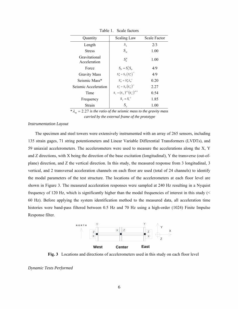
Table 1. Scale factors

Quantity Scaling Law Scale Factor

Length LS 2/3

Stress S 1.00

Gravitational Acceleration

gaS 1.00

Force 2F LS S S 4/9

Gravity Mass 1g gm F aS S S

4/9

Seismic Mass* 1s gm m mS S 0.20

Seismic Acceleration 1 s

mFsa SSS 2.27

Time 5.05.0 s

aLt SSS 0.54

Frequency 1 tf SS 1.85

Strain S 1.00

* 2.27m is the ratio of the seismic mass to the gravity mass

carried by the external frame of the prototype

Instrumentation Layout

The specimen and steel towers were extensively instrumented with an array of 265 sensors, including

135 strain gages, 71 string potentiometers and Linear Variable Differential Transformers (LVDTs), and

59 uniaxial accelerometers. The accelerometers were used to measure the accelerations along the X, Y

and Z directions, with X being the direction of the base excitation (longitudinal), Y the transverse (out-of-

plane) direction, and Z the vertical direction. In this study, the measured response from 3 longitudinal, 3

vertical, and 2 transversal acceleration channels on each floor are used (total of 24 channels) to identify

the modal parameters of the test structure. The locations of the accelerometers at each floor level are

shown in Figure 3. The measured acceleration responses were sampled at 240 Hz resulting in a Nyquist

frequency of 120 Hz, which is significantly higher than the modal frequencies of interest in this study (<

60 Hz). Before applying the system identification method to the measured data, all acceleration time

histories were band-pass filtered between 0.5 Hz and 70 Hz using a high-order (1024) Finite Impulse

Response filter.

Fig. 3 Locations and directions of accelerometers used in this study on each floor level

Dynamic Tests Performed

XY

Z

N O R T H

Z

X

Y Y

Z

X

ZX

West Center East

7

The specimen was subjected to a sequence of 44 dynamic tests including ambient-vibration tests,

free-vibration tests, and forced-vibration tests (white-noise and seismic base excitations). The main events

are shown in Table 2. The testing sequence consisted of earthquake ground motions of increasing

intensity. Before and after each earthquake record, low-amplitude white-noise base excitation tests were

performed to provide data for the study presented in this paper. The input ground motions were obtained

by scaling the time and amplitude of the ground acceleration time history recorded along the NS direction

at the Gilroy 3 station during the 1989 Loma Prieta earthquake. For structures with a fundamental

frequency close to that of the infilled frame studied here, the Gilroy 3 motion scaled at 67% corresponds

to a moderate design level earthquake for Seismic Design Category D, while the original (unscaled)

motion corresponds to a Maximum Considered Earthquake (MCE). The MCE event selected as the

reference base motion intensity in this study has spectral accelerations Ss = 1.5 g and S1 = 0.6 g, and

represents the worst case scenario for San Diego and a moderate scenario for the Los Angeles area

(ASCE 2006, Stavridis 2009). In this study, FE model updating for damage identification is performed for

seven different damage states of the structure (S0 and S2-S7). Damage state S0 (baseline) corresponds to

the uncracked state of the structure before its exposure to the first seismic base excitation, while damage

states S1 to S7 correspond to the conditions of the structure after it was subjected to different levels of the

Gilroy earthquake. Table 2 summarizes the dynamic tests and the corresponding damage states of the test

structure that are considered here.

System Identification of the Infilled Frame

The modal parameters of the specimen at each of the considered damage states are identified using

the deterministic-stochastic subspace identification (DSI) method (Van Overschee and De Moore 1996),

an input-output method, based on data from the low-amplitude (0.03g and 0.04g RMS) white-noise base

excitation tests. Output-only system identification methods, which have been successfully applied for

system identification of linear systems (He et al. 2009; Moaveni et al. 2011), are based on the assumption

of a broadband (ideal white-noise) input excitation. However, in this set of experiments, the white-noise

base excitation inputs were significantly modified by the shake table system dynamics, and consequently,

the table motions did not satisfy the broadband assumption as illustrated in Figure 4 for Test 13. The

large outdoor UCSD shake table has an oil column frequency at 10.5 Hz under bare table condition, and

the effect of the oil column resonance are mitigated through the use of a notch filter centered at 10.5 Hz in

the shake table controller. The large spectral peak just below 10 Hz (see Figure 4) can be attributed to the

dynamic interaction between the specimen and the table. More details on the mechanical and dynamic

characteristics of the shake table can be found in Ozcelik et al. (2008). The application of output-only

system identification methods to these nominal “white-noise” base excitation test data would result in

8

large estimation errors in the modal parameters, due to deviation of the input excitations from broadband

signals.

Table 2. Dynamic tests used in this study (WN: white-noise base excitation; EQ: earthquake base excitation; DE: design earthquake; MCE: maximum considered earthquake)

Test No. Test Date Test Description Damage State

5 11/3/2008 0.03g RMS WN, 5 min S0 8 “ 20% Gilroy EQ 9 “ 0.03g RMS WN, 5 min S1 12 11/6/2008 40% Gilroy EQ 13 “ 0.03g RMS WN, 5 min S2 21 11/10/2008 67% Gilroy EQ (DE) 25 11/12/2008 0.04g RMS WN, 5 min S3 26 “ 67% Gilroy EQ (DE) 27 “ 0.04g RMS WN, 5 min S4 28 “ 83% Gilroy EQ 29 “ 0.04g RMS WN, 5 min S5 33 11/13/2008 91% Gilroy EQ 34 “ 0.04g RMS WN, 5 min 35 “ 100% Gilroy EQ (MCE) 36 “ 0.04g RMS WN, 5 min S6 40 11/18/2008 120% Gilroy EQ 41 “ 0.04g RMS WN, 5 min S7

Fig. 4 Fourier Amplitude Spectrum of the base excitation measured on the shake table during Test 13

At each damage state, the DSI method has been applied to 5-minute long filtered input-output data

records. The input is the recorded acceleration on the shake table and the output data are the longitudinal,

transverse, and vertical acceleration responses of the specimen at various locations. After the records were

filtered, an input-output Hankel matrix was formed for each test including 20 block rows with 17 or 18

9

rows each (1 input and 16 or 17 output channels) and 71,962 columns. Figure 5 shows in polar plots the

complex-valued mode shapes of the four most significantly excited modes of the test structure identified

based on data from Test 5 (damage state S0). These are the first two longitudinal modes (1-L, 2-L), the

second torsional mode (2-T) and the second coupled longitudinal-torsional (2-L-T) mode. The polar plot

representation of a mode shape provides information on the degree of non-classical or non-proportional

damping (Veletsos and Ventura 1986) characteristics of that mode. If all components of a mode shape

(each component being represented by a vector in a polar plot) are collinear, the vibration mode is

classically damped. The more scattered the mode shape components are in the complex plane, the more

the structural system is non-classically damped in that mode. However, measurement noise (low signal-

to-noise ratio), estimation errors, and modeling errors can also cause a classically damped vibration mode

to be identified as non-classically damped. From Figure 5, it is observed that the 1-L, 2-L and 2-L-T

modes at damage state S0 are identified as almost perfectly classically damped, while some degree of

non-proportional damping is identified for the 2-T mode.

Fig. 5 Polar plot representation of complex mode shapes at damage state S0

The real part of the identified mode shapes are shown in Figure 6. It should be noted that the six

measurements on motions perpendicular to the infill wall plane are also used to plot the mode shapes in

Figures 5 and 6. However, Figure 6 indicates that the longitudinal mode shapes have negligible out-of-

plane components. The torsional modes were excited due to imperfections in the construction of the

specimen and in the loading conditions, such as an unintended eccentricity between the center of mass

and center of stiffness of the specimen, the small yaw rotation of the table induced by table-specimen

interaction, and the imperfect geometry and control system of the table. The natural frequencies and

damping ratios of the four most significantly excited modes are given in Table 3 for all considered

damage states. Modal Assurance Criterion (MAC) values (Allemang and Brown 1982) were also

computed to compare the complex-valued mode shapes identified at each damage state with the

corresponding mode shapes identified at damage state S0. The MAC value, bounded between 0 and 1,

measures the degree of correlation between two mode shape vectors i� and j� as

2*

22ΜΑC , )

i j

i j

i j

=� �

� �� �

( (1)

10

where * denotes the complex conjugate transpose. The reported modal parameters of the second torsional

mode (2-T) are obtained based on the longitudinal and transverse acceleration measurements, while the

other three modes are identified based on longitudinal and vertical acceleration data. This is due to the

fact that the transverse components are negligible for the longitudinal mode shapes and relatively small in

the 2-L-T mode shape. From Table 3, it is observed that the identified natural frequencies decrease

consistently with increasing level of damage, while the identified damping ratios increase. It is

noteworthy that the decrease in the natural frequencies of the two longitudinal modes with increasing

damage is much more significant than for the 2-T and 2-L-T modes. A similar observation can be made

on the increase of the identified damping ratios. The MAC values, which compare the identified mode

shapes at each damage state with their counterpart identified at state S0, also follow a monotonically

decreasing trend with increasing damage. The high MAC values (close to one) for damage states S1 to S4

indicate that there is little change in the identified mode shapes at these damage states. The identified

natural frequencies and mode shapes of the two longitudinal modes are used in the following sections to

identify the location and level of damage undergone by the infilled frame in the seismic tests.

Fig. 6 Vibration mode shapes of the infilled frame at damage state S0

Finite Element Model Updating for Damage Identification

A sensitivity-based FE model updating strategy (Friswell and Mottershead 1995; Teughels 2003;

Teughels and De Roeck 2005) is used to identify damage in the structure at various damage states. The

finite element model of the structure is divided into substructures, in each of which the damage is

assumed to be uniformly distributed. In this study, damage is defined as a relative change in the material

stiffness (effective modulus of elasticity) of the finite elements in each substructure. Therefore, the

effective modulus of elasticity is assumed to be uniform in each substructure (i.e., one effective modulus

of elasticity per sub-structure) and is updated at each considered damage state of the structure through

constrained minimization of an objective function.

11

Table 3. Modal parameters of the infilled frame identified at different damage states

Damage State: S0 S1 S2 S3 S4 S5 S6 S7

Mode 1-L

Frequency [Hz] 18.18 18.11 17.99 16.74 15.93 14.78 8.47 5.34

Damping [%] 2.0 2.4 1.9 3.3 3.8 6.1 15.7 15.6 MAC 1.00 1.00 1.00 1.00 1.00 0.98 0.80 0.71

Mode 2-T *

Frequency [Hz] 21.16 21.02 21.32 20.77 20.16 19.69 18.20 17.39 Damping [%] 1.5 1.5 1.3 1.5 1.8 1.5 1.5 1.6

MAC 1.00 1.00 1.00 0.99 0.98 0.99 0.95 0.68

Mode 2-L

Frequency [Hz] 41.22 41.09 41.56 40.21 38.56 35.50 27.34 22.57

Damping [%] 1.1 1.0 1.0 1.4 3.0 4.4 4.8 4.2 MAC 1.00 1.00 1.00 0.99 0.96 0.92 0.74 0.67

Mode 2-L-T

Frequency [Hz] 57.81 57.35 57.96 56.25 54.64 52.65 45.98 43.33 Damping [%] 1.1 1.3 1.0 0.7 1.2 2.1 2.1 2.7

MAC 1.00 1.00 1.00 0.97 0.92 0.87 0.54 0.29* Mode 2-T is identified based on longitudinal and transverse measurements

while the other three modes are identified based on longitudinal and vertical measured data

Finite Element Model of Test Structure in FEDEASLab

A linear elastic FE model of the structure is developed using the Matlab-based (MathWorks 2005)

structural analysis software FEDEASLab (Filippou and Constantinides 2004). The model consists of 35

nodes interconnected with 54 linear elastic shell and frame elements, as shown in Figure 7. A four-node

linear elastic flat shell element with four Gauss integration points available in the literature (Allman 1988;

Batoz and Taher 1982) and implemented in FEDEASLab by He (2008) is used to model the infill walls.

The beams and columns of the RC frame are modeled with Bernoulli-Euler frame elements. The

distributed mass of the structure is lumped at the nodes of its FE model. The initial FE model of the

structure is based on the geometry of the physical specimen and the elastic moduli of the concrete and

masonry measured from material tests conducted on the day of the first design level earthquake excitation

(67% Gilroy, Test 21) (Stavridis 2009). For the FE model updating, the three columns in each story of the

structure are treated as one substructure, and so are the infill walls in the two bays. Hence, the specimen is

divided into six substructures. The substructures are selected based on the number and location of the

sensors, observability of the updating parameters from the measured data, an effort to limit the total

number of updating parameters to avoid ill-conditioning, and the authors’ experience from previous FE

model updating studies (Moaveni et al. 2008; Moaveni et al. 2010). Moreover, the window openings are

ignored, and it is assumed that the solid masonry panel in the west bay and the panel with a window in the

east bay have the same modulus of elasticity and exhibit the same level of damage in each story. This is a

simplifying assumption that has been made due to the inability of the damage identification procedure to

12

distinguish between damage in the east and west panels due to similar sensitivities of the measured data to

the stiffness of the east and west bays of each floor (compensation effects between effective moduli of

elasticity in east and west bays). It should be noted that the three longitudinal accelerometers at each floor

are attached to the floor slab, which is very stiff in plane, and therefore record very similar acceleration

time histories.

Fig. 7 FE model of the RC frame structure with the six substructures used for damage identification

Objective Function

The objective function ( )f θ used for the identification of the effective material stiffness θ in each

substructure is defined as

20 0 0 2( ) ( ) ( ) ( ( ) ) ( ( ) ) [ ( ) ] [ ( ( ) ) ]T T a a

j j k k kj k

f w r w a aθ r θ W r θ a θ a W a θ a θ θ (2)

where θ is a set of physical parameters (i.e., the effective moduli of elasticity of the various

substructures), which must be adjusted to minimize the objective function; ( )r θ is the modal residual

vector containing the differences between the experimentally identified and FE predicted modal

parameters; W is a diagonal weighting matrix for modal residuals; ( )a θ is a vector of dimensionless

damage factors representing the level of damage in each of the substructures of the FE model; and 0a is

the vector of initial damage factors used as starting point in the optimization process. At each damage

state, 0a is selected as the vector of damage factors identified at the previous damage state, and 0a 0 for

the first damage state considered (S2) in the model updating procedure. The weighting matrix aW for

damage factors is a diagonal matrix with each diagonal component representing the relative cost (or

penalty) associated with the change of the corresponding damage factor. The weights for damage factors

are used for regularization and can reduce the estimation error of the damage factors in the presence of

1-Column

1-Wall

2-Column

3-Column

2-Wall

3-Wall

13

estimation uncertainty in the modal parameters, especially for substructures with parameters to which the

employed residuals are less sensitive (Mares et al. 2002). The residual vector ( )r θ in the objective

function defined in Eq. (2) contains

( ) ( ) ( )TT T

f sr θ r θ r θ (3)

in which ( )fr θ and ( )sr θ represent the eigenfrequency and mode shape residuals, respectively, defined

as

( ) ( )

( ) , ( ) ( ), {1 2 } ( )

l lj j j j

f s mr rjj j

l r j Nθ θ

r θ r θθ

� �

� � (4)

where ( )j θ and j denote the FE predicted and experimentally identified eigenvalues, respectively, for

the jth vibration mode, i.e., ( )22j jf= , in which jf is the corresponding natural frequency; ( )j θ� and

j� denote the FE predicted and experimentally identified mode shape vectors, respectively. It should be

noted that for each vibration mode, the mode shapes ( )j θ� and j� are normalized in a consistent way,

i.e., scaled with respect to the same reference component. In Eq. (4), the superscript r indicates the

reference component of a mode shape vector, the superscript l refers to the mode shape components that

are used in the FE model updating process, which in this case correspond to the degrees of freedom along

which the accelerometers measure the acceleration response of the specimen, and mN denotes the

number of vibration modes considered in the damage identification process.

In this study, the natural frequencies and mode shapes of the first two longitudinal vibration modes of

the structure are used to form the modal residual vector ( )r θ , resulting in a total of 34 residual

components which include 2 natural frequency residuals and 2× 17 -1 = 32 mode shape component

residuals based on 17 channels of acceleration response measurements. The vector ( )r θ does not include

the reference mode shape component used in the normalization. Weights of 1 and 0.5 are assigned to the

modal residuals corresponding to the natural frequencies of the first and second longitudinal modes,

respectively (i.e., 1 21, 0.5w w ). Weight factors are assigned based on the estimation uncertainty of

the natural frequency as well as the modal contribution of the corresponding mode. The first vibration

mode contributes predominantly to the dynamic response of the structure at all damage states considered,

and therefore, its corresponding residuals are assigned a larger weight than the residuals of the second

vibration mode. For each mode, the weight factors assigned to mode shape component residuals are equal

to the weight factor for the corresponding natural frequency divided by the number of mode shape

14

residuals. The damage factor weights used in the regularization are set to 10.02 0.02akw w , with

1, , subk n where subn denotes the number of substructures used in the FE model updating process.

Finally, the dimensionless damage factors used in the FE model updating process are defined as

0

, 0

S Sik k

k Si Sk

E Ea

E

-= (5)

where SikE is the effective modulus of elasticity of substructure k at damage state Si. The above damage

factors are used in the objective function introduced in Eq. (2).

Optimization Algorithm

The optimization algorithm used to minimize the objective function defined in Eq. (2) is a standard

Trust Region Newton method (Coleman and Li 1996), which is a sensitivity-based iterative method. The

optimization process was performed using the “fmincon” command from the Matlab (MathWorks 2005)

optimization toolbox, with the Jacobian matrix and a first-order estimate of the Hessian matrix calculated

based on the analytical sensitivities of the modal residuals to the updating parameters. Sensitivities of the

eigenfrequencies and mode shapes to the updating parameters are computed based on analytical solutions

provided by Fox and Kapoor (1968). It is worth mentioning that the use of the analytical Jacobian, instead

of the Jacobian estimated through finite difference calculations, increases significantly the efficiency of

the computational effort required for minimizing the objective function.

Damage Identification Results

In this study, the FE model updating procedure outlined above has been implemented to identify and

quantify damage in the test structure. The modal residual vector ( )r θ in the objective function is formed

using the natural frequencies and mode shapes of the first two longitudinal vibration modes. The first step

in the damage identification process consists of deriving a baseline FE model of the undamaged structure

(at state S0) which is used as a reference to quantify damage in the subsequent damage states. In this step,

the initial FE model, defined with data available from material tests, is updated to match as closely as

possible the identified modal parameters at the undamaged state of the structure by updating the stiffness

(effective moduli of elasticity) of the six substructures. This step is performed to account for modeling

errors as well as the possible difference between of moduli of elasticity of concrete and masonry within

each substructure and those obtained from the material tests. The updated model is termed the baseline

model to be distinguished from the initial model, which is based entirely on the material test data. The

15

modal properties of the baseline model closely match those identified from the intact structure (see the

first row of Table 5).

The effective moduli of elasticity of the different substructures of the initial and the baseline models

are summarized in Table 4. The values reported for the initial model correspond to the moduli of elasticity

of concrete and masonry infill measured from uniaxial compression tests of concrete cylinders and

masonry prisms (Stavridis 2009). Masonry prisms provide the closest representation of a masonry

assembly. The prisms used in this study consisted of four stacked brick units connected with mortar

joints. From the results reported in Table 4, it is observed that for each substructure, the baseline effective

moduli of elasticity differ from the corresponding measured (initial) values. This is due to the fact that the

updating parameters (moduli of elasticity) act as effective moduli of elasticity reflecting the overall

stiffness of the specimen, accounting for the modeling errors and the contributions of other structural

components such as beams for which the stiffness parameters are not calibrated/updated. In this study, a

simplifying assumption is made in that the masonry infill is modeled as a homogeneous isotropic

material. During the calibration of the initial FE model to obtain the baseline FE model, the “damage

factors” defined in Eq. 5 are constrained within the range [-2, 0.9].

Table 4. Effective moduli of elasticity of structural components in different substructures for the initial and baseline FE models

Substructure Effective Moduli of Elasticity [ksi]

Initial FE model Baseline FE model (S0)

1st story infills 785 722

2nd story infills 777 901

3rd story infills 946 944

1st story columns 2380 2438

2nd story columns 2530 1935

3rd story columns 2463 2263

Once the baseline model is obtained, the moduli of elasticity of the six substructures (three for infill

walls, with one per story, and three for columns, with one per story) shown in Figure 7 are updated from

the baseline FE model (at the undamaged state S0) for damage states S2, S3, S4, S5, S6 and S7. Due to

the very small changes in the modal parameters from S0 to S1, FE model updating is not performed at

state S1. The stiffness parameters of the elements representing the beams are kept constant at the values

used in the baseline FE model. This is a good approximation based on the observed behavior of the

physical specimen.

16

In updating the FE model for each considered damage state of the infilled frame, the dimensionless

damage factors are constrained to be in the range [ 0,k Sia 0.99] (k = 1, 2, …, nsub = 6). At each damage

state, the vector of initial damage factors 0Sia , used as starting point in the optimization process, is

selected as the vector of damage factors identified at the previous damage state. This lower bound is

assigned based on the assumption that the damage factors should increase monotonically as the structure

was exposed to stronger earthquakes base excitations (i.e., damage is irreversible). The damage factors

(relative to the baseline FE model) obtained at different damage states are presented in a bar plot in Figure

8. These results indicate that, as expected, the severity of structural damage increases as the structure was

exposed to stronger earthquake excitations which can be expected due to the accumulation of damage. It

is also observed from the results that the extent of the identified damage diminished in the upper stories of

the structure with severe damage concentrated in the bottom story, which is indicative of a soft story

mechanism. The first measurable damage occurs after the Design Earthquake (DE) at damage state S3,

and the largest absolute increase of the damage factor in the bottom story infilled walls (substructure 1-

Wall) occurs between damage states S5 and S6 (i.e., during the Maximum Considered Earthquake, MCE).

Fig. 8 Identified damage factors in various substructures

Table 5 reports the natural frequencies computed from the updated FE model at each considered

damage state together with their counterparts identified from white-noise base excitation test data as well

as the MAC values between the FE predicted and experimentally identified mode shapes. To compare the

mode shapes, only the degrees of freedom corresponding to the locations and orientations of the

accelerometers are used for the FE results. From Table 5, it is observed that the FE predicted natural

frequencies and mode shapes for the first two longitudinal modes match very well their experimentally

identified counterparts. Moreover, the MAC values between the FE predicted and experimentally

identified mode shapes are very close to unity for all damage states. The MAC values are in general

1−Col 2−Col 3−Col 1−Wall 2−Wall 3−Wall0

20

40

60

80

100

Dam

age

Fac

tor

[%]

Substructure

S2S3S4S5S6S7

17

higher for the first mode than for the second mode. However, this can be expected since smaller weight

factors were assigned to the modal residuals corresponding to the second mode shape.

Table 5. Comparison of FE computed and experimentally identified modal parameters

Damage State 1-L mode 2-L mode

Exp. Freq FE Freq MAC Exp. Freq FE Freq MAC

S0 (baseline) 18.18 17.92 0.99 41.22 42.61 0.96

S2 17.99 17.88 1.00 41.56 42.50 0.95

S3 16.74 16.77 1.00 40.21 40.22 0.98

S4 15.93 15.97 1.00 38.56 38.39 0.99

S5 14.78 14.82 1.00 35.50 35.33 0.99

S6 8.47 8.56 0.99 27.34 24.78 0.99

S7 5.34 5.34 0.99 22.57 22.51 0.97

(a) bay with solid panel (b) bay with window

Fig. 9 Cracks in the first story infills at damage state S3 (after 67% Gilroy)

Comparison of Damage Identification Results with Observed Damage

According to the observations made during the shake table tests, the first noticeable deterioration of

the physical specimen occurred during 67% Gilroy, which corresponds to the design earthquake for this

structure. After this event, i.e., at damage state S3, the inspection of the physical specimen revealed the

first cracks in the structure. As shown in Figure 9, cracks developed along the boundary between the solid

infill and the bounding RC frame, and cracks initiated at the window corners for the infill with a window

opening. These cracks were insignificant and did not alter significantly either the modal properties or the

integrity of the structure. This observation is consistent with the damage identification results in Figure 8,

which show very small damage factors at damage state S2, and 18% loss of stiffness in the first story

Infill-frame separation

18

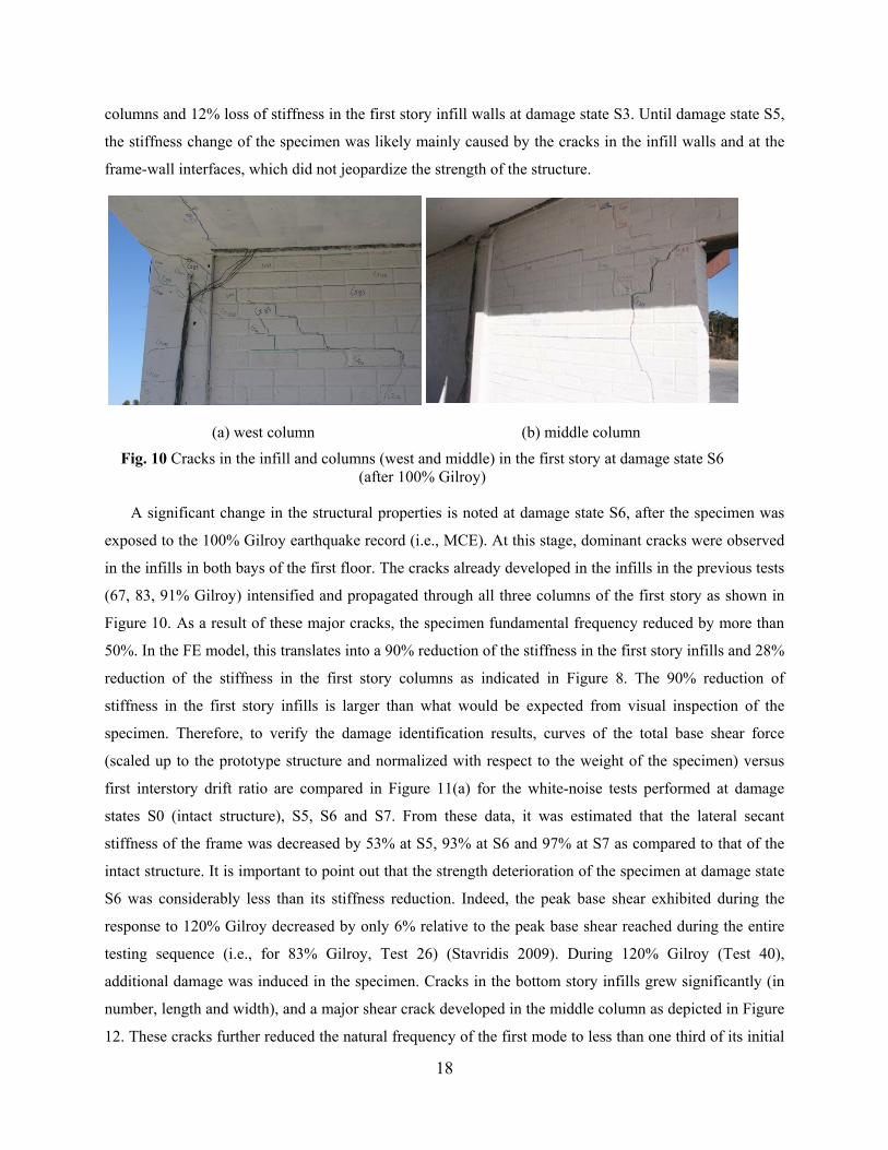
columns and 12% loss of stiffness in the first story infill walls at damage state S3. Until damage state S5,

the stiffness change of the specimen was likely mainly caused by the cracks in the infill walls and at the

frame-wall interfaces, which did not jeopardize the strength of the structure.

(a) west column (b) middle column

Fig. 10 Cracks in the infill and columns (west and middle) in the first story at damage state S6 (after 100% Gilroy)

A significant change in the structural properties is noted at damage state S6, after the specimen was

exposed to the 100% Gilroy earthquake record (i.e., MCE). At this stage, dominant cracks were observed

in the infills in both bays of the first floor. The cracks already developed in the infills in the previous tests

(67, 83, 91% Gilroy) intensified and propagated through all three columns of the first story as shown in

Figure 10. As a result of these major cracks, the specimen fundamental frequency reduced by more than

50%. In the FE model, this translates into a 90% reduction of the stiffness in the first story infills and 28%

reduction of the stiffness in the first story columns as indicated in Figure 8. The 90% reduction of

stiffness in the first story infills is larger than what would be expected from visual inspection of the

specimen. Therefore, to verify the damage identification results, curves of the total base shear force

(scaled up to the prototype structure and normalized with respect to the weight of the specimen) versus

first interstory drift ratio are compared in Figure 11(a) for the white-noise tests performed at damage

states S0 (intact structure), S5, S6 and S7. From these data, it was estimated that the lateral secant

stiffness of the frame was decreased by 53% at S5, 93% at S6 and 97% at S7 as compared to that of the

intact structure. It is important to point out that the strength deterioration of the specimen at damage state

S6 was considerably less than its stiffness reduction. Indeed, the peak base shear exhibited during the

response to 120% Gilroy decreased by only 6% relative to the peak base shear reached during the entire

testing sequence (i.e., for 83% Gilroy, Test 26) (Stavridis 2009). During 120% Gilroy (Test 40),

additional damage was induced in the specimen. Cracks in the bottom story infills grew significantly (in

number, length and width), and a major shear crack developed in the middle column as depicted in Figure

12. These cracks further reduced the natural frequency of the first mode to less than one third of its initial

19

value at state S0. At damage state S7, damage factors of 28% and 97% were identified for the first story

columns and infill walls, respectively, while a damage factor of 17% was identified for the second story

walls, which only developed minor cracks. This confirms the soft-story mechanism that developed in the

structure. The fact that the damage factor of the first story columns remains unchanged at 28% from

damage state S4 does not reflect the observed increase of damage in the columns between damages states

S4 and S7. This is likely due to the much higher sensitivity of the modal parameters to the stiffness of the

infills than to the stiffness of the columns.

(a) Hysteretic behavior of the structure during white-noise tests at damage states S0 (intact

specimen), S5, S6, and S7

(b) Hysteretic behavior of the structure during the initial cycles of response to 100% Gilroy and the

preceding white-noise test (Test 34)

Fig. 11. Base shear versus drift ratio of the first story obtained at different damage states

(a) West bay (b) East bay

Fig. 12 Observed damage in the first-story infills at damage state S7 (after 120% Gilroy)

In this approach to damage identification, damage is defined as a loss of stiffness in the structure.

Therefore, changes in natural periods and mode shapes, which reflect changes in secant stiffness

20

properties of the substructures in the FE model of the specimen, are used in the objective function for

damage identification. However, in this particular case, the actual loss of strength of the specimen is

found to be significantly less than its stiffness reduction. Furthermore, the identified damage factors are

sensitive to the amplitude of the white-noise base excitation to which the structure is assumed to respond

quasi-linearly (also found by Moaveni et al. 2010). This can be observed in Figure 11(b) which compares

the response of the specimen in terms of base shear versus first story drift ratio during the first 2.5

seconds of 100% Gilroy with that from the preceding white-noise test (Test 34). It can be seen that the

structure responded inelastically during the white noise test with a secant stiffness matching well that of

the initial part of the response to 100% Gilroy. After this low-amplitude initial response to 100% Gilroy,

the structure softened as the amplitude of its displacement increased with increasing intensity of the

earthquake excitation.

Conclusions

In this study, a linear FE model updating strategy is applied for vibration-based damage identification

of a 2/3-scale, three-story, two-bay, infilled RC frame tested on the UCSD-NEES outdoor shake table.

The objective function for damage identification is defined as a combination of natural frequency and

mode shape residuals measuring the discrepancy between experimentally identified and FE predicted

modal parameters. FE model updating is first used to calibrate the FE model at the undamaged state

which serves as the reference/baseline state, and then applied for damage identification at a number of

damage states of the structure. These damage states correspond to states of increasing damage of the

physical specimen in the process of being subjected to a sequence of earthquake excitations of increasing

intensity.

The damage identification results indicate that the severity of structural damage increases as the

structure is exposed to stronger earthquake excitations. The first significant loss of stiffness is identified at

damage state S3 (after submission of the design level earthquake) which coincides with the first

observation of cracks on the specimen. The largest increase in identified damage factors occurs between

damage states S5 and S6, i.e., due to 91% and 100% Gilroy (maximum considered earthquake). This

result is consistent with the significant reduction in the secant stiffness of the specimen that was observed

from the base shear versus first story drift hysteresis curves obtained from white-noise tests performed at

various damage states including S5 and S6. The damage identification method correctly identifies the

spatial distribution of damage in the structure, with the most severe damage at the bottom story and the

least damage at the top story. The method also captures the fact that the extent of damage is more

significant in the infill walls than in the columns. The analytical modal parameters obtained from the

21

updated FE models are in good agreement with their experimentally identified counterparts, an indication

of the accuracy of the updated FE models. However, comparison of the damage identification results and

the seismic shake table test results shows that the level of damage identified may not accurately reflect the

loss of the structural strength, as loss of stiffness (defined herein as damage) is not well related to actual

loss of strength. This motivates the need for new research based on nonlinear FE model updating where

calibrated, mechanics-based, nonlinear degrading FE models of structural systems are used to predict both

stiffness degradation and strength deterioration.

The following conclusions are drawn from this study and previous work performed by the authors.

The damage factors obtained using a linear FE model updating approach, are sensitive to the amplitude of

the white-noise base excitation to which the structure is assumed to respond quasi-linearly. With

increasing level of base excitation and structural damage, the level of nonlinearity in the structural

response increases. Therefore, the assumption that the structure behaves as a quasi-linear dynamic system

is violated and a linear dynamic model is not strictly able to represent well the behavior of a damaged

structure. The spatial distribution (i.e., relative amplitudes) of the identified damage factors however is

not sensitive to the amplitude of base excitation. Lastly, it should be mentioned that the accuracy and

spatial resolution of the damage identification results depend significantly on the accuracy and

completeness of the identified modal parameters (Moaveni et al. 2009a). The estimation

variability/uncertainty of the modal parameters can be influenced by several factors such as the number

and types of sensors, measurement noise, length of the data time windows used for system identification,

and system identification method used (Moaveni et al. 2007), in addition to the environmental conditions

such as the ambient air temperature and relative humidity during data collection (Moaveni et al. 2009b;

Moser and Moaveni 2011). The variability in the identified modal parameters due to non-damage related

factors needs to be smaller than the changes in these parameters due to damage or compensated for in

order to identify the actual damage in the structure.

Acknowledgements

The shake table tests discussed in this paper were supported by the National Science Foundation

Grant No. 0530709 awarded under the George E. Brown, Jr. Network for Earthquake Engineering

Simulation (NEES) program. Input from other collaborators at Stanford University and the University of

Colorado at Boulder, and a Professional Advisory Panel (PAP) during the planning, design, and

performance of these shake table tests is gratefully acknowledged. The panel members are David

Breiholz, John Kariotis, Gregory Kingsley, Joe Maffei, Ron Mayes, Paul Murray, and Michael Valley.

Also, the writers would like to thank the technical staff at the Englekirk Structural Engineering Center of

22

UCSD and Mr. Ioannis Koutromanos for their assistance in the shake table tests. The opinions expressed

in this paper are those of the authors and do not necessarily represent those of the NSF, the collaborators,

or the PAP.

REFERENCES

ASCE (2006). “Minimum design loads for buildings and other structures.” ASCE/SEI 7-05, Reston, Va.

Allemang, R. J., and Brown, D. L. (1982). “A correlation coefficient for modal vector analysis.” Proc. of 1st International Modal Analysis Conference, Bethel, Connecticut.

Allman, D.J. (1988). “A quadrilateral finite element including vertex rotations for plane elasticity analysis.” International Journal for Numerical Methods in Engineering, 26(3), 717-730.

Batoz, J.L., and Tahar, M.B. (1982). “Evaluation of a new quadrilateral thin plate bending element.” International Journal for Numerical Methods in Engineering, 18(11), 1655-1677.

Coleman, T.F., and Li, Y. (1996). “An interior, trust region approach for nonlinear minimization subject to bounds.” SIAM Journal on Optimization, 6(2), 418-445.

Doebling, S.W., Farrar, C.R., Prime, M.B., and Shevitz, D.W. (1996). Damage identification in structures and mechanical systems based on changes in their vibration characteristics: a detailed literature survey. Los Alamos National Laboratory Report, LA-13070-MS, Los Alamos, New Mexico, USA.

Doebling, S.W., Farrar, C.R., and Prime, M.B. (1998). “A summary review of vibration-based damage identification methods.” The Shock and Vibration Digest, 30(2), 99-105.

Filippou, F.C., and Constantinides, M. (2004). FEDEASLab getting started guide and simulation examples. Technical Report, NEESgrid-2004-22, http://fedeaslab.berkeley.edu.

Fox, R.L., and Kapoor, M.P. (1968). “Rates of change of eigenvalues and eigenvectors.” AIAA Journal, 6(12), 2426-2429.

Friswell, M.I., and Mottershead, J.E. (1995). Finite element model updating in structural dynamics. Kluwer Academic Publishers, Boston, USA.

He, X. (2008). Vibration-based damage identification and health monitoring of civil structures. Ph.D. thesis, Department of Structural Engineering, University of California, San Diego.

He, X., Moaveni, B., Conte, J.P., Elgamal A., and Masri, S.F. (2009). “System identification of Alfred Zampa Memorial Bridge using dynamic field test data.” Journal of Structural Engineering, ASCE, 135(1), 54-66.

Koutromanos, I., Stavridis, A., and Shing, P.B. (2011). “Numerical modeling of masonry-infilled RC frames subjected to seismic loads.” Journal of Computers and Structures, in press (available online).

Mares, C., Friswell, M.I., and Mottershead, J.E. (2002). “Model updating using robust estimation.” Mechanical Systems and Signal Processing, 16(1), 169-183.

MathWorks Inc. (2005). Matlab - High performance numeric computation and visualization software, User’s Guide. The MathWorks Inc., Natick, MA.

Moaveni, B., Barbosa, A.R., Conte, J.P., Hemez, F.M. (2007). “Uncertainty analysis of modal parameters obtained from three system identification methods.” Proc. of International Conference on Modal Analysis (IMAC-XXV), Orlando, FL.

Moaveni, B., Conte, J.P., and Hemez, F.M. (2009a). “Uncertainty and sensitivity analysis of damage identification results obtained using finite element model updating.” Journal of Computer Aided Civil and Infrastructure Engineering, 24(5), 320-334.

23

Moaveni, B., He, X., Conte J.P., and De Callafon, R.A. (2008). “Damage identification of a composite beam using finite element model updating.” Journal of Computer Aided Civil and Infrastructure Engineering, 23(5), 339-359.

Moaveni, B., He, X., Conte, J.P., Fraser, M., and Elgamal, A. (2009b). “Uncertainty analysis of Voigt Bridge modal parameters due to changing environmental condition.” Proc. of International Conference on Modal Analysis (IMAC-XXVII), Orlando, FL, USA.

Moaveni, B., He, X., Conte, J.P., and Restrepo, J.I. (2010). “Damage identification study of a seven-story full-scale building slice tested on the UCSD-NEES shake table.” Structural Safety, 32(5), 347-356.

Moaveni, B., He, X., Conte, J.P., Restrepo, J.I., and Panagiotou, M. (2011). “System identification study of a seven-story full-scale building slice tested on the UCSD-NEES shake table.” Journal of Structural Engineering, ASCE, in press, doi:10.1061/(ASCE)ST.1943-541X.0000300.

Moser, P., and Moaveni, B. (2011). “Environmental effects on the identified natural frequencies of the Dowling Hall Footbridge.” Mechanical Systems and Signal Processing, in press, doi:10.1016/j.ymssp.2011.03.005.

Ozcelik, O., Luco, J.E., Conte, J.P., Trombetti, T.L., and Restrepo, J.I. (2008). “Experimental characterization, modeling and identification of the NEES-UCSD shake table mechanical system.” Earthquake Engineering and Structural Dynamics, 37(2), 243-264.

Reynders, E., De Roeck, G., Bakir, P.G., and Sauvage, C. (2007). “Damage identification on the Tilff bridge by vibration monitoring using optical fibre strain sensors.” Journal of Engineering Mechanics, ASCE, 133(2), 185-193.

Sohn, H., Farrar, C.R., Hemez, F.M., Shunk, D.D., Stinemates, D.W., and Nadler, B.R. (2003). A review of structural health monitoring literature: 1996-2001. Los Alamos National Laboratory Report, LA-13976-MS, Los Alamos, New Mexico, USA.

Stavridis, A. (2009). Analytical and experimental seismic performance assessment of masonry-infilled RC frames. Ph.D. Dissertation, Department of Structural Engineering, University of California, San Diego, CA.

Stavridis, A., and Shing, P.B. (2010). “Finite element modeling of nonlinear behavior of masonry

infilled RC frames.” Journal of Structural Engineering, ASCE. 136(3), 285-296.

Teughels A. (2003). Inverse modelling of civil engineering structures based on operational modal data. Ph.D. Dissertation, Department of Civil Engineering, K.U. Leuven, Belgium.

Teughels, A., and De Roeck, G. (2004). “Structural damage identification of the highway bridge Z24 by finite element model updating.” Journal of Sound and Vibration, 278(3), 589–610.

Teughels, A., and De Roeck, G. (2005). “Damage detection and parameter identification by finite element model updating.” Archives of Computational Methods in Engineering, 12(2), 123–164.

Van Overschee, P., and de Moore, B. (1996). Subspace identification for linear systems. Kluwer Academic Publishers, Boston, Massachusetts, USA.

Veletsos, A.S., and Ventura, C.E. (1986). “Modal analysis of non-classically damped linear systems.” Earthquake Engineering and Structural Dynamics, 14(2), 217-243.

Zhou, X.T., Ko, J.M., and Ni, Y.Q. (2007). “Experimental study on identification of stiffness change in a concrete frame experiencing damage and retrofit.” Structural Engineering and Mechanics, 25(1), 39-52.