daniel le maire - econstor.eu
TRANSCRIPT
econstorMake Your Publications Visible.
A Service of
zbwLeibniz-InformationszentrumWirtschaftLeibniz Information Centrefor Economics
Albæk, Karsten; Leth-Petersen, Søren; Le Maire, Daniel; Tranæs, Torben
Working Paper
Does Peacetime Military Service Affect Crime?
IZA Discussion Papers, No. 7528
Provided in Cooperation with:IZA – Institute of Labor Economics
Suggested Citation: Albæk, Karsten; Leth-Petersen, Søren; Le Maire, Daniel; Tranæs, Torben(2013) : Does Peacetime Military Service Affect Crime?, IZA Discussion Papers, No. 7528,Institute for the Study of Labor (IZA), Bonn
This Version is available at:http://hdl.handle.net/10419/80515
Standard-Nutzungsbedingungen:
Die Dokumente auf EconStor dürfen zu eigenen wissenschaftlichenZwecken und zum Privatgebrauch gespeichert und kopiert werden.
Sie dürfen die Dokumente nicht für öffentliche oder kommerzielleZwecke vervielfältigen, öffentlich ausstellen, öffentlich zugänglichmachen, vertreiben oder anderweitig nutzen.
Sofern die Verfasser die Dokumente unter Open-Content-Lizenzen(insbesondere CC-Lizenzen) zur Verfügung gestellt haben sollten,gelten abweichend von diesen Nutzungsbedingungen die in der dortgenannten Lizenz gewährten Nutzungsrechte.
Terms of use:
Documents in EconStor may be saved and copied for yourpersonal and scholarly purposes.
You are not to copy documents for public or commercialpurposes, to exhibit the documents publicly, to make thempublicly available on the internet, or to distribute or otherwiseuse the documents in public.
If the documents have been made available under an OpenContent Licence (especially Creative Commons Licences), youmay exercise further usage rights as specified in the indicatedlicence.
www.econstor.eu

DI
SC
US
SI
ON
P
AP
ER
S
ER
IE
S
Forschungsinstitut zur Zukunft der ArbeitInstitute for the Study of Labor
Does Peacetime Military Service Affect Crime?
IZA DP No. 7528
July 2013
Karsten AlbækSøren Leth-PetersenDaniel le MaireTorben Tranæs

Does Peacetime Military Service Affect Crime?
Karsten Albæk SFI – The Danish National Centre for Social Research
Søren Leth-Petersen
University of Copenhagen and SFI
Daniel le Maire University of Copenhagen
Torben Tranæs
Rockwool Foundation Research Unit, CESifo and IZA
Discussion Paper No. 7528 July 2013
IZA
P.O. Box 7240 53072 Bonn
Germany
Phone: +49-228-3894-0 Fax: +49-228-3894-180
E-mail: [email protected]
Any opinions expressed here are those of the author(s) and not those of IZA. Research published in this series may include views on policy, but the institute itself takes no institutional policy positions. The IZA research network is committed to the IZA Guiding Principles of Research Integrity. The Institute for the Study of Labor (IZA) in Bonn is a local and virtual international research center and a place of communication between science, politics and business. IZA is an independent nonprofit organization supported by Deutsche Post Foundation. The center is associated with the University of Bonn and offers a stimulating research environment through its international network, workshops and conferences, data service, project support, research visits and doctoral program. IZA engages in (i) original and internationally competitive research in all fields of labor economics, (ii) development of policy concepts, and (iii) dissemination of research results and concepts to the interested public. IZA Discussion Papers often represent preliminary work and are circulated to encourage discussion. Citation of such a paper should account for its provisional character. A revised version may be available directly from the author.
IZA Discussion Paper No. 7528 July 2013
ABSTRACT
Does Peacetime Military Service Affect Crime?* Draft lottery data combined with Danish longitudinal administrative records show that military service can reduce criminal activity for youth offenders who enter service at ages 19-22. For this group property crime is reduced for up to five years from the beginning of service, and the effect is therefore not only a result of incapacitation while enrolled. We find no effect of service on violent crimes. We also find no effect of military service on educational attainment and unemployment, but we find negative effects of service on earnings. These results suggest that military service does not upgrade productive human capital directly, but rather impacts criminal activity through other channels, for example by changing the attitudes to criminal activity for this group. JEL Classification: H56, K42, J24 Keywords: crime, military service, activation
NON-TECHNICAL SUMMARY Peacetime military service seems to affect the future life of young men both positively and negatively. It reduces the criminal activities both during and after military serves for young men that already had a criminal record when enrolled. But this positive effect comes at a cost, because young men who do military service seem to earn less after the service than comparable young men who do not serve. Corresponding author: Torben Tranæs The Rockwool Foundation Research Unit Sølvgade 10, 2. tv. 1307 Copenhagen K. Denmark E-mail: [email protected]
* Daniel le Maire is grateful for financial support from the Danish Social Science Research Council.

2
1. Introduction
Crime is costly for society and there is ongoing debate about how to reduce youth crime. The aim of
this paper is to measure the effect of peacetime military service by conscription on the propensity to
commit crime during and after service. Peace time conscription is widespread. For example, many
NATO countries have peace time conscription. One of the objectives of conscription is to support
democracy by improving civil-military relations and by educating youth by offering them a new
chance in life, introducing them to other segments of the population, and informing them about
important civil values, Sørensen (2000). By teaching obedience and discipline military service may
also provide skills that are potentially directly relevant in the labor market and, thereby, make labor
market activity more attractive relative to criminal activity. Furthermore, the fact that military service
occupies the time of the conscripts while in service can potentially also contribute to reducing crime.
Military service can thus potentially impact criminal behavior by incapacitation, by affecting
productive human capital, and by socializing conscripts towards being better citizens, i.e. shaping their
attitude towards criminal activity. Military service can, however, also enhance criminal behavior by
delaying labor market entry and education thereby worsening labor market opportunities. What is
more, training in the use of weapons may stimulate criminal activity. Finally, conscription is
associated with close and long term interaction with new peers, and this can affect criminal behavior
both positively and negatively depending on the quality of the peers.
The literature about the effect of peacetime military service on crime is sparse. Galiani et al. (2011)
estimate the effect of military service by conscription in Argentina, during war as well as peace time,
on the propensity to commit crime. Identifying the causal effect by exploiting the randomization of
eligibility inherent in the draft lottery, they find that military service increases the propensity to
develop a subsequent criminal record and that service has a detrimental effect on subsequent labor
market performance. Effects are more adverse for individuals having served during war time. A
related strand of literature has examined the association between war veteran status and subsequent
criminal activity, see MacLean and Elder (2007) for an overview. The evidence from this literature is

3
mixed and seems to depend on the context. A number of papers show that military service can impact
other important aspects of people’s lives. Angrist (1990) exploits the Vietnam War draft lottery to
show that Vietnam veterans earn less than otherwise similar men who were not drafted. Follow-up
studies have found earnings effects to be short lived, Angrist, Chen and Song (2011) and Angrist and
Chen (2011), although the latter study finds that the GI Bill generated schooling gains for veterans.
Angrist (1998) shows evidence that voluntary military service can have positive effects on post-
service employment. Card and Cardoso (2012) show evidence that peace time conscription increases
the earnings of low-skilled Portuguese men.
A range of studies have tried to quantify the effect of various policy initiatives on reducing crime.
Some policy measures have obvious short-lived effects. For example, imprisonment takes the criminal
out of criminal activity (at least outside the prison) and increased police effort also seems to lower
criminal activity, Chalfin and McCrary (2013). Much of the previous evidence about how to reduce
crime has focused on the effect of schooling and social policies. The literature about the effect of
schooling is much too large to give a full account of here and we refer to Lochner (2011) who surveys
effects of schooling and job training programs on crime. Schooling can generally affect crime directly
by upgrading human capital and changing opportunity costs of crime or by occupying time and
thereby reducing crime through incapacitation. It can also affect crime by changing the attitude
towards criminal activity by affecting the psychic rewards, preferences for risk taking or patience, or
by affecting social interaction. There appears to be evidence that human capital upgrading has lasting
effects. For example, in a recent paper Machin, Marie, and Vujic (2011) exploit an increase in the
minimum schooling age from age 15 to 16 in 1972-73 in England and Wales and find that the effect of
one year of additional schooling reduces property crime by 20-30% over the period 1972-1996. There
is also evidence that incapacitation plays a role. Jacob and Lefgren (2003) examine juvenile crime
rates on days when school is not in session with days when it is and find that crime rates are higher
when school is not in session. Similarly, Luallen (2006) finds that crime rates are higher when teachers
strike. A number of studies have also found that pre-school programs can have sizeable long run

4
effects, Lochner (2011). Social policies may also affect the propensity to commit crime. For example,
in a recent study Fallesen et al. (2012) investigate the effect of labor market programs activating
unemployed workers on crime and find that activation reduces criminal activity significantly and that
the effect is not only the result of incapacitation by reducing leisure hours since criminal activity is
also reduced on weekends when leisure hours are not affected. Educational and social programs are,
however, difficult to design so as to reach high risk groups such as youth offenders, and peace time
military service by conscription may be a way of reaching such groups.
This paper focuses on the effect of peacetime military service on criminal activity. To identify the
causal effect of military service we exploit the fact that all young men in Denmark upon reaching the
age of 18 are liable to participate in a draft lottery for military service. Exploiting this source of
randomization we ensure that we are not considering a particular type of young men in military
service, i.e. our estimates are not plagued by self-selection into service. This research design is similar
to the design applied by Galiani et al. (2011) and Angrist and coauthors. Our data are longitudinal
covering the 1964 cohort from the year the individuals turn 16 and the next 20 years forward. It
includes information about convictions, schooling, labor market attachment, earnings and family
background. By observing pre-conscription convictions we are able to identify youth offenders and to
estimate effects separately for this group. The longitudinal data also allow us to characterize the
dynamic effects of military service on subsequent criminal activity.
Our results show that peace time military service lowers the propensity to commit property crime
among youth offenders, i.e. young people who had committed crime before they entered military
service. For this group property crime is reduced for up to five years from the beginning of service,
and the effect is, therefore, not only a result of incapacitation while enrolled. Criminal activity in
Denmark peaks at age 18 and is reduced to about half of this by age 251 and most efforts to reduce
crime target people aged 16-25. Our results suggest that military service can reduce crime for youth
1 This is documented by Statistics Denmark, http://www.statbank.dk/statbank5a/default.asp?w=1301. Similar patterns are well-known for other countries, e.g. Imai and Krishna (2004) and Grogger (1998).
5
offenders for a significant fraction of the criminal intensive age interval. We do not find any effects on
violent crimes. We speculate that this is because violent crimes are acts of impulse while property
crimes often are the result of unsentimental planning, Jacob and Lefgren (2003). We do not find any
effects of military service on post-service educational attainment or on employment, and we find that
service leads to lower earnings for up to four years after completed service. These results suggest that
military service does not upgrade productive human capital directly, but rather impacts criminal
activity through other channels, for example by changing the attitude to criminal activity for this group
Our study provides new evidence about the impact of peace-time military conscription on criminal
activity. The only previous study of peace-time conscription on criminal activity, Galiani et al. (2011),
found that service boosted subsequent criminal activity. We find that military service has no effect on
crime for the vast majority of conscripts. Unlike Galiani et al. (2011) we are able to identify youth
offenders and to examine whether effects are different for this sub-group who are at risk of continuing
a criminal career. Our results suggest that this is indeed the case. Youth offenders who are randomized
into military service have lower crime rates for up to five years from the beginning of service than
youth offenders who are not in service. This new evidence suggests that peace time military service by
conscription may be a way to reach a high-risk group that is otherwise difficult to reach using other
policy measures.
The next section describes the Danish military service and draft lottery as well as the data and the
ability of the draft lottery number to predict military service. The following section briefly outlines the
methodology. Section 4 presents the results and section 5 sums up and concludes the analysis.
2. Military Service and data
Military service
All Danish men upon reaching the age of 18 become liable for conscription and participate in a draft
lottery for national service. The draft lottery takes place in connection with a conscription examination

6
where participants are also subjected to a health examination and an IQ test. The IQ test is used for
identifying individuals who are not eligible for service, see Teasdale (2009).2 National service
includes military and civil defense service. The vast majority of inductees participate in military
service, and we will simply refer to it as military service. The lottery has numbers corresponding to the
size of the cohort attending the draft lottery in the entire country. Draft examinations are identical
across examination stations and the lottery is designed to generate an identical risk of being inducted
across the country. Men drawing a low number are inducted. How many inductees are needed depends
on the staffing needs of the military and civil defense as well as on the number of volunteers. In
practice, men are called for induction up to a ceiling corresponding to about 25-30% of the cohort. The
exact number is, however, unknown at the time of the lottery.
In our sample about 16% are not eligible for military service. Some of these never participate in the
lottery because they are obviously not qualified for service. This could, for example, be because they
have obvious physical disabilities or mental problems rendering them unable to participate in service.
Some participate in the lottery but are subsequently assessed to be unfit for service because of health
problems that did not disqualify them at first or because they have very low test scores. In fact, when
we compare observed characteristics of the group of ineligibles with those who are eligible, the test
scores are the only factor for which we can trace significant differences between these two groups.3 In
particular, there is no difference between the eligible and ineligible group in terms of youth crime.
The link between the lottery number and the execution of service is not deterministic because not all
men who draw a number turn out to be eligible. There is also a small group of draft resisters, who,
after having participated in the draft lottery, resist military service. Draft resisters are assigned to non-
military service in various places, for example kindergartens, libraries, NGOs, or municipal
administration/service. It is possible to volunteer, and volunteering for service can either be true
volunteering or technical volunteering where participants can decide to volunteer after having drawn a 2 The test has been validated extensively, see Teasdale et al. (2011), and it has been shown to have satisfactory test-retest reliability, to correlate with other acknowledged IQ tests and to not be influenced by motivational effects from the conscription context. 3 We do not have information about health in our data.

7
low number that would obviously imply induction. Technical volunteering can be advantageous
because volunteers can expect more influence on the service in terms of the type of service (army,
navy, air force, civil defense), which could influence both the length and nature, as well as the
geographic location, of the service. Volunteering can, thereby, also affect the timing of service as
some types of service have waiting lists. The timing of participation in the conscription examination
and service can also be influenced by educational deferment. The lottery number thus randomizes
entry into military service but does not randomize the timing of entry.
Data
We use merged administrative data for this study. The core data set consists of draft lottery records for
all men born in 1964 and residing in the eastern part of Denmark4 thereby covering 42% of the 1964
cohort. Participation in the conscription examination is concentrated in the years 1982-1984.5 Besides
the lottery number we have access to test scores as well as measures of body weight and height from
the health examination. All lottery numbers are recorded together with the Central Person Registry
(CPR) number. This number is also the key for recording information in all public administrative
registers and we are therefore able to merge lottery numbers with yearly information from a range of
other administrative registers. In particular, we merge lottery records with criminal records from the
Central Crime Register. This data set holds information about all arrests made by the Danish police,
the charges filed against individuals and subsequent verdicts. In the analysis we consider an individual
to have committed a crime if he is convicted, and we thus do not consider charges leading to
acquittal.6 The criminal records provide less detail in the early part of the sample period. For example,
before 1990, only the year that the criminal act took place is recorded. The crime records allow us to
distinguish between violent crimes and property crimes. We divide the sample according to whether 4 Specifically, all males born in 1964 and residing in municipalities with a municipality code smaller than 400 according to Statistics Denmark’s official municipal code system. 5 Participation in the conscription examination is distributed as follows: 1982: 14%, 1983: 57%, 1984: 18% 1985:7%, later: 4%. 6 Charges which the police withdraw due to lack of evidence are not considered, but when charges are withdrawn due to other considerations such as the age of the defendant we include them in the analysis.
8
the individuals committed crime before 1982, i.e. at the age of 15-17 years. We will refer to those
committing crime in 1980-1981 as youth offenders.
We merge crime and conscription examination records with income tax records and with a range of
other registers containing information about education and family background. As administrative
registers are longitudinal we collect information for these individuals to cover the period 1980-1999.
Unfortunately, we do not have direct recording of whether people have entered military service. In
constructing the data we assign a given individual to military service if he has been recorded as a wage
earner at a military facility during a given year. Draft examination records contain information about
the semester in which a person attended the conscription examination, and we identify military service
from employment at a military facility in the same or subsequent semesters. This procedure potentially
involves some error in the measurement of military service and the relationship between military
service and the lottery number will not be deterministic. Furthermore, military service lasts for 3-12
months for regular service depending on the type of service, but can be up to 24 months for
individuals selected to go through training to become officers, and service can begin at different points
in time during the year, but we do not have information to distinguish between these cases. This
implies that if military service begins towards the end of the year and extends into a new calendar
year, then the conscript will be recorded as being in service for two consecutive years.
We focus on individuals who participated in the lottery and who are assessed to be eligible for service.
This leaves us with 11,563 individuals of which 4,548 entered military service. Table 1 presents
descriptive statistics for the sample. The focus of the paper is on whether military service affects the
propensity to commit crime. In the analysis we are going to separately consider youth offenders, i.e.
individuals who have received a sentence before service, and individuals without a criminal record,
and the table therefore presents descriptive statistics for these two groups separately. The idea is that
youth offenders are at higher risk of committing crime again and the potential for reducing criminal
activity is, therefore, greater for this group. Unsurprisingly, youth offenders are more likely to commit
crimes than individuals who are not youth offenders, and most of the criminal activity is property
crime. Compared to non-offending youths, youth offenders also have less education, their parents have
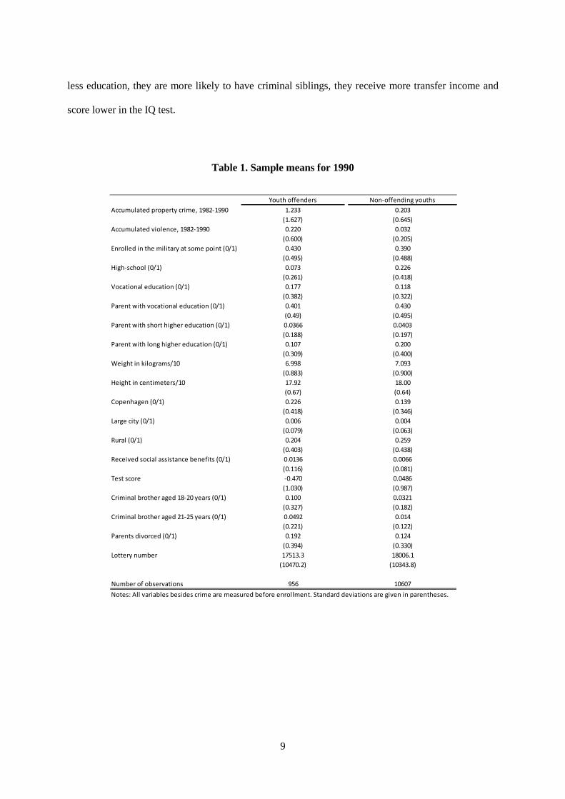
9
less education, they are more likely to have criminal siblings, they receive more transfer income and
score lower in the IQ test.
Table 1. Sample means for 1990
Youth offenders Non-offending youthsAccumulated property crime, 1982-1990 1.233 0.203
(1.627) (0.645)Accumulated violence, 1982-1990 0.220 0.032
(0.600) (0.205)Enrolled in the military at some point (0/1) 0.430 0.390
(0.495) (0.488)High-school (0/1) 0.073 0.226
(0.261) (0.418)Vocational education (0/1) 0.177 0.118
(0.382) (0.322)Parent with vocational education (0/1) 0.401 0.430
(0.49) (0.495)Parent with short higher education (0/1) 0.0366 0.0403
(0.188) (0.197)Parent with long higher education (0/1) 0.107 0.200
(0.309) (0.400)Weight in kilograms/10 6.998 7.093
(0.883) (0.900)Height in centimeters/10 17.92 18.00
(0.67) (0.64)Copenhagen (0/1) 0.226 0.139
(0.418) (0.346)Large city (0/1) 0.006 0.004
(0.079) (0.063)Rural (0/1) 0.204 0.259
(0.403) (0.438)Received social assistance benefits (0/1) 0.0136 0.0066
(0.116) (0.081)Test score -0.470 0.0486
(1.030) (0.987)Criminal brother aged 18-20 years (0/1) 0.100 0.0321
(0.327) (0.182)Criminal brother aged 21-25 years (0/1) 0.0492 0.014
(0.221) (0.122)Parents divorced (0/1) 0.192 0.124
(0.394) (0.330)Lottery number 17513.3 18006.1
(10470.2) (10343.8)
Number of observations 956 10607Notes: All variables besides crime are measured before enrollment. Standard deviations are given in parentheses.

10
The timing of service is not fixed, among other things because of educational deferment. Figure 1
shows the distribution of the timing of service for our sample. Most individuals enter service between
19 and 22 years of age.
Figure 1. Distribution of age at enrollment
3. Methods and first-stage
When estimating the effect of military service on crime using OLS, a major concern is that enrollment
is correlated with omitted personal characteristics. This potential endogeneity arises because of the
option to join the military voluntarily. To address this concern, we estimate the effect with 2SLS using
the lottery number as an instrument for military service. One requirement for the lottery number to be
a valid instrument is that it should be able to predict military service, such that a lower number is
associated with higher probability of service. For draft lottery numbers to be valid instruments they
must also be uncorrelated with potential outcomes in and out of military service. This assumption can
be plausibly defended by alluding to the randomization by the draft lottery. Our military enrollment
0
500
1000
1500
2000
2500
18 19 20 21 22 23 24 25 26 27

11
dummy is measured with error because we have to infer it from payroll records. Draft resisters are an
example of this as we do not know whether they are recorded as enrolled or not. However, the number
of draft resisters is small7 and we do not expect this to be quantitatively important for our analysis.
Another requirement for the instrument to be valid is, therefore, that the lottery number is uncorrelated
with this type of measurement error. The validity of the orthogonality assumption is not directly
verifiable, but we conduct a test for validity of the overidentifying restrictions, and if the measurement
error in military service does not have the required properties, then this test should be rejected. To
estimate the causal effect of military service we are confined to the subsample consisting of eligibles
having participated in the lottery. Under these assumptions our estimates can be interpreted as Local
Average Treatment Effects (LATE). Our methodology is similar to the one applied by Angrist and
Chen (2011). Estimates generated by using lottery number instruments are informative about the effect
in the population of eligible men who draw lottery numbers. As a consequence we do not have much
to say about the effect among true volunteers, for example.
Although the lottery number randomizes individuals between treatment and control groups, it does not
randomize the timing of the military service. Therefore, we need to rely on an estimation where we do
not use the timing of enrollment. One possibility is to accumulate the committed crime over the period
starting at the point of the draft examination, that is 1982-1990, and regress this on whether the
individuals were serving in the military at some point, as well as some covariates measures before
1982. That is
𝑐𝑟𝑖𝑚𝑒 1982−1990,𝑖 = 𝛽0 + 𝛽1𝑀𝑖𝑙𝑖𝑡𝑎𝑟𝑦1982−1990,𝑖 + 𝑋1980−1981,𝑖𝛽2 + 𝑢𝑖 (1)
7 The total number of draft resisters in the full population was 466 in 1982 declining to 218 in 1986. Assuming that draft resisters are equally distributed across the country we would expect about 1-200 resisters in our sample. We assign military service from employment at a military facility. If resisters are recorded at a military facility they will be classified as being in service and if they are not then they will be recorded as not being in service, but we do not know this.

12
where i indexes the individual, 𝑐𝑟𝑖𝑚𝑒 1982−1990,𝑖 is the accumulated crime, 𝑀𝑖𝑙𝑖𝑡𝑎𝑟𝑦1982−1990,𝑖 is a
dummy variable taking the value one if individual i joins the military at some point between 1982 and
1990. This estimation will only reveal whether military service has had an effect on criminal activity,
but it does not reveal, for example, whether the military only has an incapacitation effect or whether
military service has longer-lived effects.
To unfold the time pattern of the effect of military enrollment, we separately estimate a series of
equations which make use of the panel dimension to estimate effects of military service for up to eight
years after the point of enrollment. To focus on a homogenous group, our treatment group is
individuals who join the military at the ages of 19-22 years. This group corresponds to 92 percent of
the all persons eventually enrolled. We follow the cohort being 19-22 years when enrolled over time.
For example, to estimate the second-year effects of military enrollment, we include this cohort in their
second year since military enrollment, and as control group we use all individuals aged 20-23 who
have not been enrolled. Therefore, we repeatedly estimate equations of the following form,
𝑐𝑟𝑖𝑚𝑒 𝑖𝑡 = 𝛽0 + 𝛽1𝑀𝑖𝑙𝑖𝑡𝑎𝑟𝑦19−22,𝑖𝑡 + 𝑋1980−1981,𝑖𝛽2 + 𝑡𝑖𝑚𝑒𝑑𝑢𝑚𝑚𝑖𝑒𝑠 + 𝑢𝑖𝑡 (2)
As the dependent variable in equation (2) is a dummy variable, 2SLS suffers from the usual problems
associated with linear probability models that probabilities are not confined to the [0;1] interval. We
therefore also present results from estimating the model using a bivariate probit estimator not suffering
from this problem, but at the cost of imposing joint normality of the errors.
Figure 2 shows the relationship between the lottery number and the frequency of military service. 80-
86% of all men with a lottery number lower than 7,000 end up in military service. For numbers
between 7,000 and 20,000 the frequency of military service declines steadily and for numbers above
20,000 the frequency levels at approximately 20%. As noted above, there is not a deterministic link
between the lottery number and our measure of military service and this is likely to be the reason that
we do not observe complete participation even among people with low lottery numbers in our sample
consisting of eligible men. The pattern in figure 2 is not affected by the inclusion of covariates (not

13
reported). When specifying the first-stage for estimating equation (1) we approximate the shape in
figure 2 by a function composed of a constant in the interval [1;7000[, a second degree polynomial in
the interval [7000;20000[ and a constant in the interval [20000; 35000]. This provides overidentifying
restrictions that can be used to test the validity of the assumption that the lottery number is not
correlated with the measurement error associated with the military enrollment variable.
Figure 2. Enrollment probability and lottery number
In the analysis we consider youth offenders and non-offending youths separately, and the results from
estimating the first stage regression using the polynomial described above are presented for these two
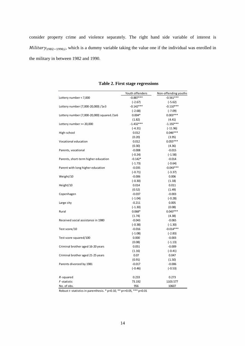
groups separately in table 2. Results show that the draft lottery number clearly predicts enrollment for
both groups.
4. Results
Results from estimating equation (1) are given in Table 3. The dependent variable is accumulated
criminal offenses 1982-1990, which cover the years where the 1964 cohort served in the military. We
0
0,1
0,2
0,3
0,4
0,5
0,6
0,7
0,8
0,9
1
1 4000 8000 12000 16000 20000 24000 28000 32000 36000
14
consider property crime and violence separately. The right hand side variable of interest is
𝑀𝑖𝑙𝑖𝑡𝑎𝑟𝑦1982−1990,𝑖, which is a dummy variable taking the value one if the individual was enrolled in
the military in between 1982 and 1990.
Table 2. First stage regressions
Youth offenders Non-offending youthsLottery number < 7,000 -0.887*** -0.561*** (-2.67) (-5.62)Lottery number (7,000-20,000) /1e3 -0.142*** -0.110*** (-2.68) (-7.09)Lottery number (7,000-20,000) squared /1e6 0.004* 0.003*** (1.82) (4.41)Lottery number >= 20,000 -1.432*** -1.192*** (-4.31) (-11.96)High-school 0.012 0.046*** (0.20) (3.95)Vocational education 0.012 0.055*** (0.30) (4.36)Parents, vocational -0.008 -0.015 (-0.24) (-1.58)Parents, short-term higher education -0.142* -0.014 (-1.73) (-0.64)Parent with long higher education -0.035 -0.043*** (-0.71) (-3.37)Weight/10 -0.006 0.006 (-0.30) (1.18)Height/10 0.014 0.011 (0.52) (1.49)Copenhagen -0.037 -0.003 (-1.04) (-0.28)Large city -0.211 0.005 (-1.30) (0.08)Rural 0.068* 0.043*** (1.74) (4.38)Received social assistance in 1980 -0.043 -0.065 (-0.38) (-1.30)Test score/10 -0.016 -0.014*** (-1.08) (-2.83)Test score squared/100 0.000 -0.003 (0.08) (-1.13)Criminal brother aged 16-20 years 0.051 -0.009 (1.16) (-0.41)Criminal brother aged 21-25 years 0.07 0.047 (0.91) (1.50)Parents divorced by 1981 -0.017 -0.006
(-0.46) (-0.53)
R -squared 0.233 0.273F -statistic 73.192 1103.577No. of obs. 956 10607Robust t -statistics in parenthesis. * p<0.10, ** p<=0.05, *** p<0.01

15
For youth offenders, we see that military service reduces the number of property crime offenses both
according to OLS and the 2SLS estimates. However, we find no significant effects for violent crime
for any of the groups.
Table 3. Accumulated crime 1982-1990
In general, the parameter estimates for the control variables have the expected signs. The effects of the
control variables tend to be more significant for property crime than violent crime, so we will only
briefly consider the control variables for property crime. First, human capital, whether in the form of
OLS 2SLS OLS 2SLS OLS 2SLS OLS 2SLSMilitary enrollment -0.243** -0.426** 0.016 0.03 -0.063 -0.086 -0.001 -0.002 (-2.39) (-2.00) (1.29) (1.20) (-1.64) (-1.11) (-0.24) (-0.21)High-school -0.439*** -0.423*** -0.080*** -0.081*** -0.100** -0.093** -0.013** -0.013** (-2.75) (-2.72) (-5.00) (-4.99) (-2.47) (-2.35) (-2.16) (-2.10)Vocational education -0.248** -0.243** 0.033 0.031 -0.011 -0.002 0.017** 0.017** (-2.02) (-2.00) (1.44) (1.38) (-0.23) (-0.05) (2.11) (2.17)Parents, vocational -0.171 -0.174 -0.034** -0.032** -0.069 -0.077* -0.005 -0.005 (-1.47) (-1.52) (-2.09) (-2.00) (-1.53) (-1.73) (-0.91) (-0.89)Parents, short-term higher education -0.162 -0.174 -0.059** -0.055** 0.011 0.018 -0.017** -0.017** (-0.77) (-0.83) (-2.32) (-2.17) (0.14) (0.23) (-2.32) (-2.31)Parents, long-term higher education -0.266 -0.280* -0.037** -0.036** -0.120*** -0.121*** -0.011** -0.011** (-1.55) (-1.65) (-2.08) (-1.99) (-2.63) (-2.68) (-2.19) (-2.18)Weight/10 -0.059 -0.061 -0.032*** -0.031*** 0.095*** 0.080** 0.005* 0.005* (-0.77) (-0.81) (-3.81) (-3.72) (2.94) (2.57) (1.68) (1.77)Height/10 -0.097 -0.094 -0.007 -0.008 -0.043 -0.037 -0.004 -0.004 (-0.93) (-0.91) (-0.55) (-0.61) (-1.03) (-0.92) (-0.81) (-0.95)Copenhagen -0.052 -0.062 0.112*** 0.112*** -0.167*** -0.166*** 0.012 0.011 (-0.39) (-0.47) (4.85) (4.84) (-3.95) (-3.98) (1.62) (1.55)Large city 1.501 1.485 0.018 0.031 -0.066 -0.012 -0.003 -0.001 (1.35) (1.36) (0.17) (0.29) (-0.37) (-0.07) (-0.13) (-0.02)Rural -0.395*** -0.384*** -0.055*** -0.055*** -0.087 -0.088* -0.007* -0.008* (-3.16) (-3.09) (-4.04) (-4.04) (-1.64) (-1.70) (-1.73) (-1.85)Received social assistance in 1980 0.799* 0.822* 0.037 0.036 0.380* 0.383* -0.014 -0.014 (1.87) (1.88) (0.49) (0.48) (1.70) (1.72) (-0.94) (-0.93)Test score -0.149*** -0.154*** -0.057*** -0.055*** -0.035 -0.026 -0.012*** -0.012*** (-2.93) (-3.04) (-6.00) (-5.87) (-1.52) (-1.17) (-3.66) (-3.59)Test score squared 0.058*** 0.059*** 0.042*** 0.042*** 0.019 0.017 0.007 0.006 (3.07) (3.10) (3.82) (3.77) (1.47) (1.35) (1.57) (1.46)Criminal brother aged 16-20 years 0.302* 0.303* 0.236*** 0.236*** 0.086 0.073 0.02 0.019 (1.82) (1.85) (4.05) (4.05) (1.08) (0.95) (1.17) (1.09)Criminal brother aged 21-25 years 0.495* 0.516* 0.078 0.079 0.213 0.204 0.013 0.012 (1.76) (1.86) (1.32) (1.34) (1.57) (1.55) (0.50) (0.46)Parents divorced by 1981 0.114 0.113 0.128*** 0.126*** -0.057 -0.037 0.019*** 0.019*** (0.85) (0.84) (5.56) (5.48) (-1.34) (-0.91) (2.70) (2.69)
R -squared 0.077 0.074 0.049 0.049 0.07 0.068 0.014 0.014P -value, Hansen J -statistic 0.903 0.562 0.164 0.758No. of obs. 956 956 10607 10607 956 956 10607 10607Robust t -statistics in parenthesis. * p<0.10, ** p<=0.05, *** p<0.01
Property crime Violent crimeYouth offenders Non-offending youths Youth offenders Non-offending youths

16
education or test scores, decreases the likelihood of committing crime. Second, the individual’s
criminal activity is also influenced by the family. If brothers committed crime in 1980-1981, this tends
to increase the propensity to commit crime later on. For non-offending youths, we find that parental
divorce contributes to increasing the likelihood of committing crime, but divorce does not seem to
affect the propensity to commit crime for individuals who as youths have already committed crime.
Finally, we find that living in rural areas is associated with a smaller propensity to commit crime.
We have performed tests for validity of the overidentifying restrictions in the case of 2SLS estimations
and these tests are never rejected at any conventional level of significance. This suggests that the
lottery number instruments do not violate the orthogonality condition and that the estimates presented
in table 3 can plausibly be interpreted as causal effects.
The magnitude of the parameter estimates suggests that over the course of 1982-1990 military service
reduced criminal activity among youth offenders in the order of 0.4 crimes over the course of the data
period.8 Comparing this with the level of accumulated property crimes among youth offenders, c.f.
table 1, this amounts to a reduction in criminal activity of about 30%. However, some individuals
joined the military in the beginning of the sample period 1982-1990 whereas others enrolled at the
end, and for some individuals the accumulated crime is therefore potentially committed prior to
enrollment. Furthermore, the estimates in table 3 do not reveal whether, for example, the effect of
military service on property crime is solely an incapacitation effect.
In table 4, we examine the time effect of military enrollment more closely. To accomplish this, we
estimate a sequence of models of the form of equation (2) exploring the dynamic pattern of property
crime for youth offenders, the only group for whom we found significant effects of military service on
crime in table 3. Figure 1 showed that only a few men enter the military relatively late, but that the
vast majority enters service at ages 19-22 and we choose to focus on these age groups in order to have
relatively homogenous treatment and control groups from which to identify dynamic effects. Table 4 8 If we extend the sample period we get further away from the most common time of enrollment and our parameter estimate for military enrollment becomes insignificant, first at the 5 percent level and when we extend the sample further also at the 10 percent level. This is likely because crime generally decreases drastically as the people get older.

17
reports the parameter estimates from a sequence of regressions where the dependent variable is
measured at different distances from the time of military service. The OLS estimates are small and
insignificant throughout. 2SLS estimates are negative but larger in magnitude than OLS and
significant for up to five years after the year of enrollment in military service, albeit the fifth year
effect is only significant at the 10 percent level. Hence, military service seems to reduce crime for
youth offenders and the effect is present not only while in service but also for a considerable period
after the service has been completed. Marginal effects are also economically significant as military
service appears to lower property crime rates by 20 percent in the first year and about 10 percent in the
fifth year. Results from applying probit and bivariate probit are qualitatively comparable to OLS and
2SLS, but marginal effects are typically lower.
In table 4 we also report estimates of the effect of military service on crime one and two years before
military service actually takes place. If the draft lottery truly randomizes people into the military
independently of their criminal behavior, we would not expect to find any effects prior to service.
Reassuringly, 2SLS estimates and bivariate probit estimates reported in table 4 confirm that this is in
fact the case, suggesting that the estimated effect of military service is not spurious.
Table 4. Property crime for youth offenders aged 19-22 at the time of enrollment
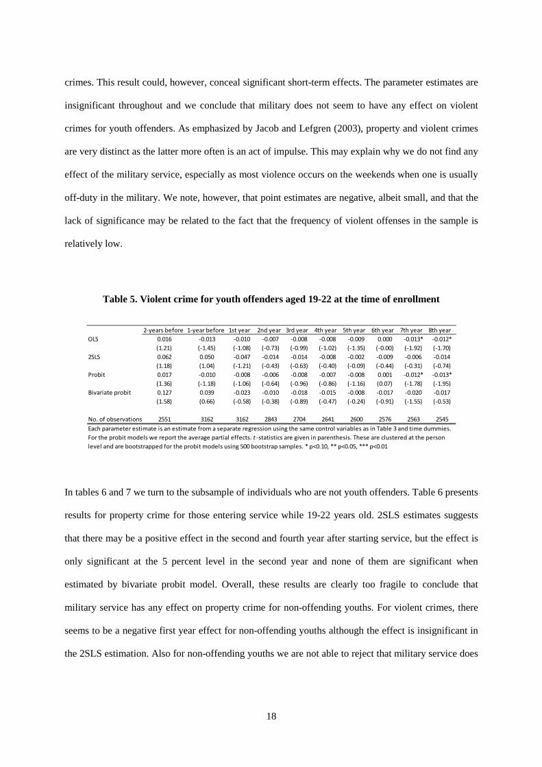
Table 5 repeats the estimation from table 4 but focuses on violent crimes for youth offenders. In table
3 we did not find any evidence that military service reduced the propensity to ever commit violent
2-years before 1-year before 1st year 2nd year 3rd year 4th year 5th year 6th year 7th year 8th yearOLS -0.051** 0.005 -0.027 -0.025 -0.019 -0.014 -0.033* -0.018 -0.022 -0.020
(-2.35) (0.24) (-1.36) (-1.28) (-1.02) (-0.72) (-1.81) (-0.97) (-1.23) (-1.18)2SLS -0.15 -0.127 -0.222** -0.155** -0.113** -0.113** -0.106* -0.041 -0.009 0.010
(-1.47) (-1.40) (-2.39) (-2.24) (-1.97) (-2.02) (-1.91) (-0.72) (-0.16) (0.21)Probit -0.049** 0.004 -0.027 -0.026 -0.021 -0.014 -0.034** -0.020 -0.022 -0.019
(-2.29) (0.18) (-1.35) (-1.32) (-1.23) (-0.78) (-2.11) (-1.14) (-1.23) (-1.22)Bivariate probit -0.098 -0.081 -0.138*** -0.103** -0.067 -0.083** -0.035 -0.022 -0.021 0.001
(-1.33) (-1.37) (-3.93) (-2.46) (-1.34) (-2.28) (-0.55) (-0.46) (-0.49) (0.03)
No. of observations 2551 3162 3162 2843 2704 2641 2600 2576 2563 2545Each parameter estimate is an estimate from a separate regression using the same control variables as in Table 3 and time dummies. For the probit models we report the average partial effects. t -statistics are given in parenthesis. These are clustered at the person level and are bootstrapped for the probit models using 500 bootstrap samples. * p<0.10, ** p<0.05, *** p<0.01
18
crimes. This result could, however, conceal significant short-term effects. The parameter estimates are
insignificant throughout and we conclude that military does not seem to have any effect on violent
crimes for youth offenders. As emphasized by Jacob and Lefgren (2003), property and violent crimes
are very distinct as the latter more often is an act of impulse. This may explain why we do not find any
effect of the military service, especially as most violence occurs on the weekends when one is usually
off-duty in the military. We note, however, that point estimates are negative, albeit small, and that the
lack of significance may be related to the fact that the frequency of violent offenses in the sample is
relatively low.
Table 5. Violent crime for youth offenders aged 19-22 at the time of enrollment
In tables 6 and 7 we turn to the subsample of individuals who are not youth offenders. Table 6 presents
results for property crime for those entering service while 19-22 years old. 2SLS estimates suggests
that there may be a positive effect in the second and fourth year after starting service, but the effect is
only significant at the 5 percent level in the second year and none of them are significant when
estimated by bivariate probit model. Overall, these results are clearly too fragile to conclude that
military service has any effect on property crime for non-offending youths. For violent crimes, there
seems to be a negative first year effect for non-offending youths although the effect is insignificant in
the 2SLS estimation. Also for non-offending youths we are not able to reject that military service does
2-years before 1-year before 1st year 2nd year 3rd year 4th year 5th year 6th year 7th year 8th yearOLS 0.016 -0.013 -0.010 -0.007 -0.008 -0.008 -0.009 0.000 -0.013* -0.012*
(1.21) (-1.45) (-1.08) (-0.73) (-0.99) (-1.02) (-1.35) (-0.00) (-1.92) (-1.70)2SLS 0.062 0.050 -0.047 -0.014 -0.014 -0.008 -0.002 -0.009 -0.006 -0.014
(1.18) (1.04) (-1.21) (-0.43) (-0.63) (-0.40) (-0.09) (-0.44) (-0.31) (-0.74)Probit 0.017 -0.010 -0.008 -0.006 -0.008 -0.007 -0.008 0.001 -0.012* -0.013*
(1.36) (-1.18) (-1.06) (-0.64) (-0.96) (-0.86) (-1.16) (0.07) (-1.78) (-1.95)Bivariate probit 0.127 0.039 -0.023 -0.010 -0.018 -0.015 -0.008 -0.017 -0.020 -0.017
(1.58) (0.66) (-0.58) (-0.38) (-0.89) (-0.47) (-0.24) (-0.91) (-1.55) (-0.53)
No. of observations 2551 3162 3162 2843 2704 2641 2600 2576 2563 2545Each parameter estimate is an estimate from a separate regression using the same control variables as in Table 3 and time dummies. For the probit models we report the average partial effects. t -statistics are given in parenthesis. These are clustered at the person level and are bootstrapped for the probit models using 500 bootstrap samples. * p<0.10, ** p<0.05, *** p<0.01

19
not affect crime before service and we conclude that the data does not reject the hypothesis that the
lottery number randomizes people into military service irrespective of their criminal behavior.
Table 6. Property crime for non-offending youths aged 19-22 at the time of enrollment
Table 7. Violent crime for non-offending youths aged 19-22 at the time of enrollment
The effect of military service on education, unemployment and earnings for youth offenders
The results presented so far suggest that military service reduces the property crime rate among youth
offenders who start military service at ages 19-22. Criminal activity is reduced not only while in
service but also for up to five years from the beginning of service, i.e. for three to four years after
2-years before 1-year before 1st year 2nd year 3rd year 4th year 5th year 6th year 7th year 8th yearOLS 0.003 0.003 0.003 0.003 0.002 0.004 0.001 0.002 -0.005** -0.001
(0.80) (1.07) (1.15) (0.92) (0.73) (1.35) (0.59) (0.74) (-2.36) (-0.40)2SLS 0.024* 0.018 0.015 0.019** 0.012 0.013* 0.006 0.007 -0.005 -0.002
(1.68) (1.50) (1.20) (2.02) (1.57) (1.90) (0.96) (1.15) (-0.77) (-0.36)Probit 0.002 0.003 0.003 0.003 0.002 0.003 0.002 0.002 -0.005** -0.001
(0.72) (1.08) (1.26) (0.94) (0.79) (1.44) (0.74) (0.83) (-2.36) (-0.37)Bivariate probit 0.013 0.009 0.003 0.012 0.008 0.008 -0.001 0.007 -0.006* -0.004
(0.91) (0.82) (0.29) (1.20) (1.03) (1.23) (-0.15) (0.95) (-1.68) (-1.06)
No. of observations 29027 36335 36325 33013 31319 30537 30080 29820 29635 29485No. of treated 3063 3820 3827 3822 3811 3807 3794 3774 3758 3745Each parameter estimate is an estimate from a separate regression using the same control variables as in Table 3 and time dummies. For the probit models we report the average partial effects. t -statistics are given in parenthesis. These are clustered at the person level and are bootstrapped for the probit models using 500 bootstrap samples. * p<0.10, ** p<0.05, *** p<0.01
2-years before 1-year before 1st year 2nd year 3rd year 4th year 5th year 6th year 7th year 8th yearOLS 0.000 -0.001 -0.002** 0.000 0.002 0.001 0.000 0.000 -0.001* 0.002
(0.36) (-0.62) (-2.56) (-0.11) (1.46) (0.69) (0.40) (0.22) (-1.66) (1.53)2SLS 0.001 0.000 -0.006 -0.001 0.004 0.003 0.000 0.003 0.002 0.006*
(0.17) (-0.05) (-1.60) (-0.21) (1.29) (0.95) (-0.03) (1.11) (0.68) (1.96)Probit 0.001 -0.001 -0.002*** 0.000 0.002 0.001 0.001 0.000 -0.001 0.002
(0.43) (-0.70) (-2.87) (0.07) (1.43) (0.75) (0.59) (0.14) (-1.59) (1.44)Bivariate probit 0.003 -0.001 -0.004*** 0.000 0.006 0.000 -0.001 0.000 0.000 0.004
(0.17) (-0.46) (-3.13) (0.06) (0.82) (-0.13) (-0.64) (0.17) (0.05) (1.22)
No. of observations 29027 36335 36325 33013 31319 30537 30080 29820 29635 29485No. of treated 3063 3820 3827 3822 3811 3807 3794 3774 3758 3745Each parameter estimate is an estimate from a separate regression using the same control variables as in Table 3 and time dummies. For the probit models we report the average partial effects. t -statistics are given in parenthesis. These are clustered at the person level and are bootstrapped for the probit models using 500 bootstrap samples. * p<0.10, ** p<0.05, *** p<0.01
20
service is completed. This could, for example, be because the military has provided skills that are
relevant for participating in the labor market, or because it has provided a set of skills that lower the
costs of investing in post-service education. We therefore go on to investigate whether the reduction in
criminal activity is associated with increased education, and/or a drop in post-service unemployment
and whether it affects earnings. This analysis is confined to youth offenders as we found no clear
effect of military enrollment for individuals not committing crime before the age of 18.
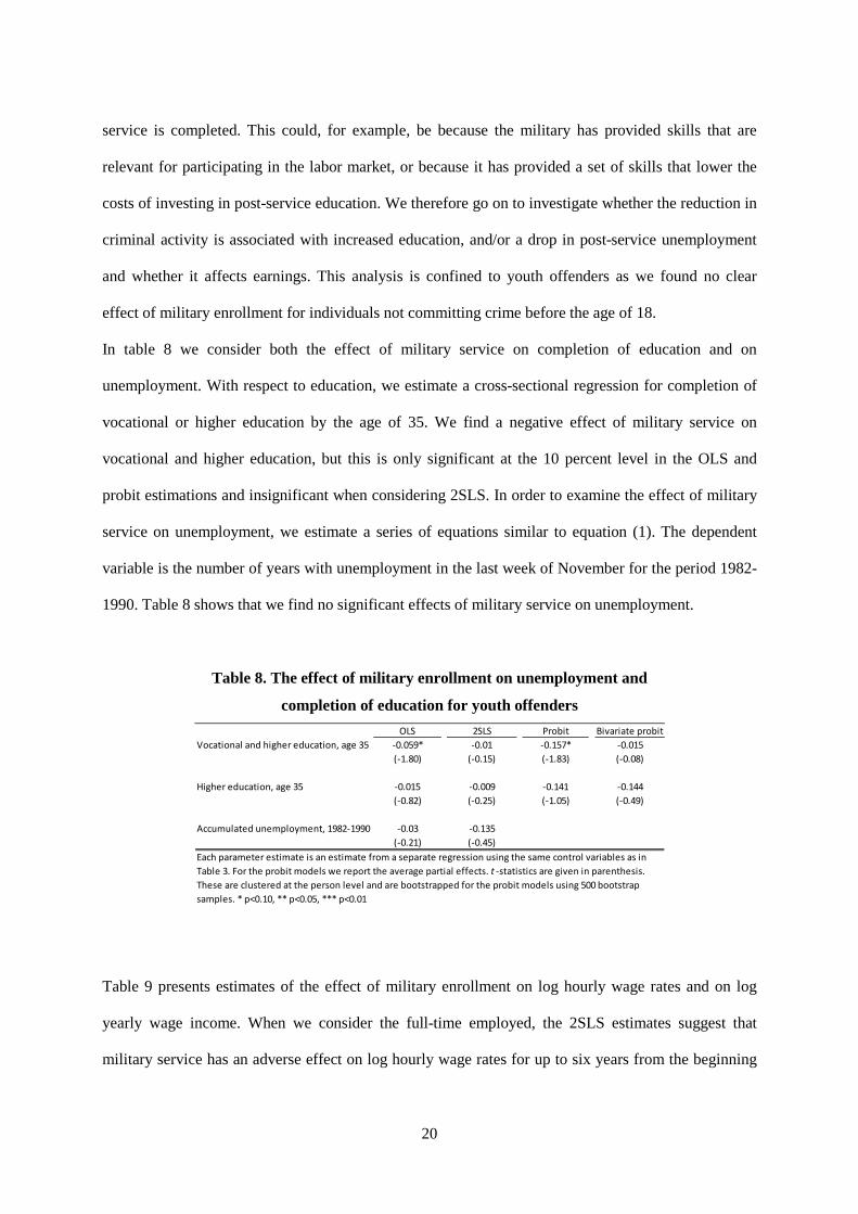
In table 8 we consider both the effect of military service on completion of education and on
unemployment. With respect to education, we estimate a cross-sectional regression for completion of
vocational or higher education by the age of 35. We find a negative effect of military service on
vocational and higher education, but this is only significant at the 10 percent level in the OLS and
probit estimations and insignificant when considering 2SLS. In order to examine the effect of military
service on unemployment, we estimate a series of equations similar to equation (1). The dependent
variable is the number of years with unemployment in the last week of November for the period 1982-
1990. Table 8 shows that we find no significant effects of military service on unemployment.
Table 8. The effect of military enrollment on unemployment and
completion of education for youth offenders
Table 9 presents estimates of the effect of military enrollment on log hourly wage rates and on log
yearly wage income. When we consider the full-time employed, the 2SLS estimates suggest that
military service has an adverse effect on log hourly wage rates for up to six years from the beginning
OLS 2SLS Probit Bivariate probitVocational and higher education, age 35 -0.059* -0.01 -0.157* -0.015
(-1.80) (-0.15) (-1.83) (-0.08)
Higher education, age 35 -0.015 -0.009 -0.141 -0.144(-0.82) (-0.25) (-1.05) (-0.49)
Accumulated unemployment, 1982-1990 -0.03 -0.135(-0.21) (-0.45)
Each parameter estimate is an estimate from a separate regression using the same control variables as in Table 3. For the probit models we report the average partial effects. t -statistics are given in parenthesis. These are clustered at the person level and are bootstrapped for the probit models using 500 bootstrap samples. * p<0.10, ** p<0.05, *** p<0.01
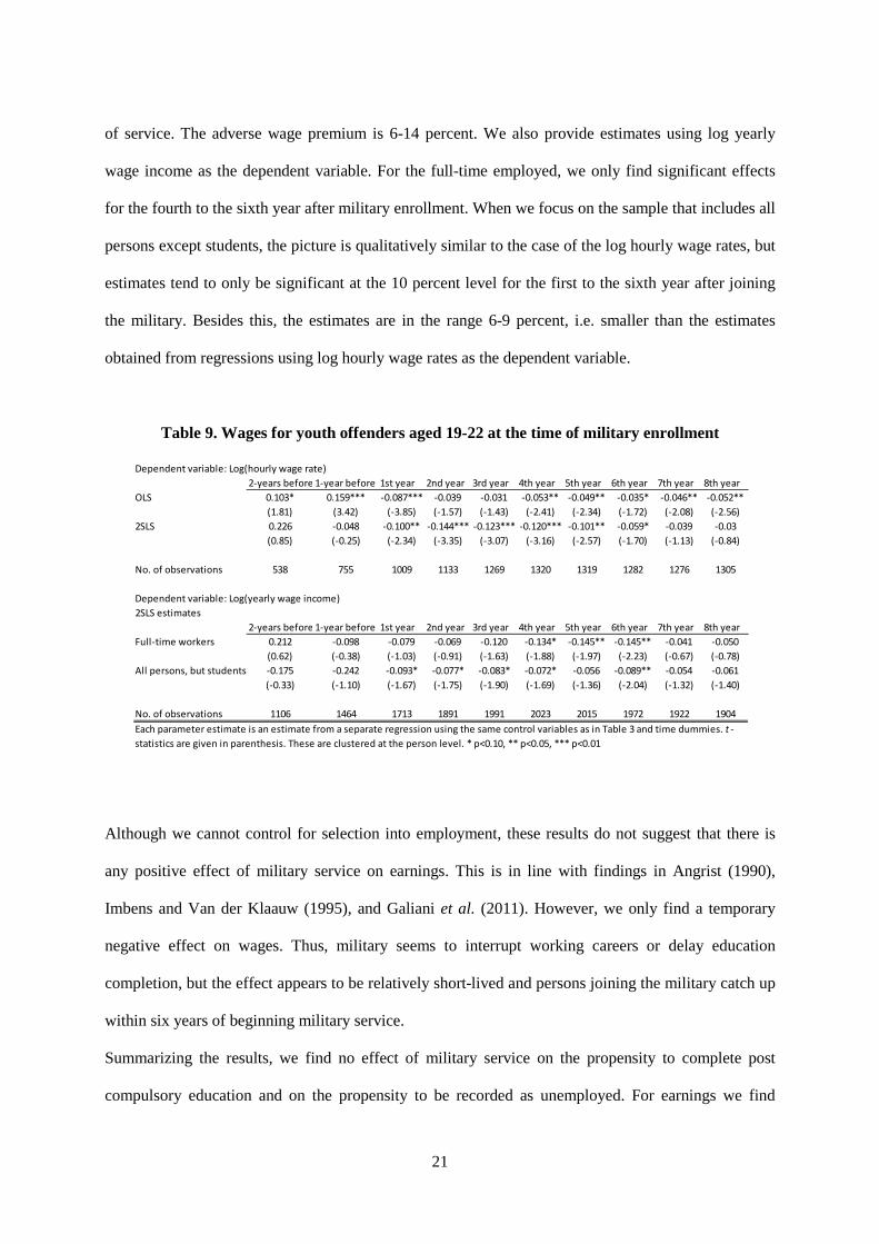
21
of service. The adverse wage premium is 6-14 percent. We also provide estimates using log yearly
wage income as the dependent variable. For the full-time employed, we only find significant effects
for the fourth to the sixth year after military enrollment. When we focus on the sample that includes all
persons except students, the picture is qualitatively similar to the case of the log hourly wage rates, but
estimates tend to only be significant at the 10 percent level for the first to the sixth year after joining
the military. Besides this, the estimates are in the range 6-9 percent, i.e. smaller than the estimates
obtained from regressions using log hourly wage rates as the dependent variable.
Table 9. Wages for youth offenders aged 19-22 at the time of military enrollment
Although we cannot control for selection into employment, these results do not suggest that there is
any positive effect of military service on earnings. This is in line with findings in Angrist (1990),
Imbens and Van der Klaauw (1995), and Galiani et al. (2011). However, we only find a temporary
negative effect on wages. Thus, military seems to interrupt working careers or delay education
completion, but the effect appears to be relatively short-lived and persons joining the military catch up
within six years of beginning military service.
Summarizing the results, we find no effect of military service on the propensity to complete post
compulsory education and on the propensity to be recorded as unemployed. For earnings we find
2-years before 1-year before 1st year 2nd year 3rd year 4th year 5th year 6th year 7th year 8th yearOLS 0.103* 0.159*** -0.087*** -0.039 -0.031 -0.053** -0.049** -0.035* -0.046** -0.052**
(1.81) (3.42) (-3.85) (-1.57) (-1.43) (-2.41) (-2.34) (-1.72) (-2.08) (-2.56)2SLS 0.226 -0.048 -0.100** -0.144*** -0.123*** -0.120*** -0.101** -0.059* -0.039 -0.03
(0.85) (-0.25) (-2.34) (-3.35) (-3.07) (-3.16) (-2.57) (-1.70) (-1.13) (-0.84)
No. of observations 538 755 1009 1133 1269 1320 1319 1282 1276 1305
2SLS estimates2-years before 1-year before 1st year 2nd year 3rd year 4th year 5th year 6th year 7th year 8th year
Full-time workers 0.212 -0.098 -0.079 -0.069 -0.120 -0.134* -0.145** -0.145** -0.041 -0.050(0.62) (-0.38) (-1.03) (-0.91) (-1.63) (-1.88) (-1.97) (-2.23) (-0.67) (-0.78)
All persons, but students -0.175 -0.242 -0.093* -0.077* -0.083* -0.072* -0.056 -0.089** -0.054 -0.061(-0.33) (-1.10) (-1.67) (-1.75) (-1.90) (-1.69) (-1.36) (-2.04) (-1.32) (-1.40)
No. of observations 1106 1464 1713 1891 1991 2023 2015 1972 1922 1904Each parameter estimate is an estimate from a separate regression using the same control variables as in Table 3 and time dummies. t -statistics are given in parenthesis. These are clustered at the person level. * p<0.10, ** p<0.05, *** p<0.01
Dependent variable: Log(hourly wage rate)
Dependent variable: Log(yearly wage income)

22
negative effects within the first six years of beginning service. Combining these findings suggests that
military service does not equip youth offenders with productive human capital.
Conclusion
We have analyzed the effect of military service on the propensity to commit crime for the cohort of
Danish men born in 1964. We address the self-selection into military service by exploiting draft lottery
data, and measure the effect of military service by combining these data with longitudinal
administrative records. The results show that military service reduces criminal activity for youth-
offenders who enter service at ages 19-22. For this group property crime is reduced for up to five years
from the beginning of service, and the effect is therefore not only a result of incapacitation while
enrolled. We find no effect of military service on violent crimes. We also find no effect of military
service on educational attainment and unemployment for youth offenders, but we find negative effects
of service on earnings. We find no effect of military service on the criminal activity of non-offending
youths. Overall, these results suggest that military service has an effect on the criminal behavior of
youth-offenders. The effect exists not because military service upgrades productive human capital
directly but rather because military service does something else, for example changes their attitude
towards criminal activity. Criminal activity peaks at age 18 and is reduced to about half by age 25.
Most efforts to reduce crime are targeted at youths in the age span 16-25. Our results thus suggest that
military service can reduce crime for youth offenders for a significant fraction of the criminal intensive
age interval.
Many European countries have compulsory military service. One of the objectives of military service
based on conscription is to inform conscripts about important civil values and to create a national
community. The results presented here suggest that military service may have beneficial effects on
youth-criminals through socialization, a positive effect that has been largely overlooked up to this
point. The results from this study also have broader relevance in terms of fighting crime. Evidence
about the effect of social policies is mixed. Our results suggest that youth offenders, a group that can

23
be difficult to reach with school and social programs, can be reached with programs that share the
features of peace time military service.

24
References
Angrist, J.D. (1990): Lifetime Earnings and the Vietnam Era Draft Lottery: Evidence from Social Security Administrative Records, American Economic Review, Vol. 80, pp. 313–335.
Angrist, J.D. (1998): Estimating the Labor Market Impact of Voluntary Military Service Using Social Security Data on Military Applicants, Econometrica, Vol. 66(2), pp. 249–288.
Angrist, J.D. and S.H. Chen (2011): Schooling and the Vietnam-Era GI Bill: Evidence from the Draft Lottery, American Economic Journal: Applied Economics, Vol. 3, pp. 96–119.
Angrist, J.D., S.H. Chen and J. Song (2011): Long-term Consequences of Vietnam-Era Conscription: New Estimates Using Social Security Data, American Economic Review, Vol. 101(3), pp. 334–338.
Card, D. and A.R. Cardoso (2012): Can Compulsory Military Service Raise Civilian Wages? Evidence from the Peacetime Draft in Portugal, American Economic Journal: Applied Economics, Vol. 4(4), pp. 57–93.
Chalfin, A. and J. McCrary (2013): The Effect of Police on Crime: New Evidence from US Cities 1960-2010, NBER WP 18815.
Fallesen, P., L.P. Geerdsen, S. Imai and T. Tranæs (2012): The Effect of Workfare Policy on Crime, Youth Diligence and Law Obedience; Rockwool Foundation Research Unit, Study Paper no. 41, University Press of Southern Denmark.
Galiani, S., M.A. Rossi and E. Schargrodsky (2011): Conscription and Crime: Evidence from the Argentine Draft Lottery, American Economic Journal: Applied Economics, Vol. 3, pp. 119–136.
Grogger, J. (1998): Market Wages and Youth Crime, Journal of Labor Economics, Vol. 16(4), pp. 756-791.
Imai, S. and K. Krishna (2004): Employment and Crime in a Dynamic Model, International Economic Review, Vol. 45(3), pp. 845-872.
Imbens, G. and W.H. Van der Klaauw (1995): Evaluating the Cost of Conscription in the Netherlands, Journal of Business and Economic Statistics, Vol. 13(2), pp. 207–215.
Jacob, B.A. and L. Lefgren (2003): Are Idle Hands the Devil's Workshop? Incapacitation, Concentration and Juvenile Crime, American Economic Review, vol. 93, no. 5, pp. 1560–1577.
Lochner, L. (2011): Nonproduction Benefits of Education: Crime, Health, and Good Citizenship, Handbook of the Economics of Education, Vol. 4, pp. 183–282.
Luallen, J. (2006) School’s Out… Forever: A Study of Juvenile Crime, At-Risk Youths and Teacher Strikes, Journal of Urban Economics, Vol. 59, pp. 75–103.
Machin, S., O. Marie and S. Vujic (2011): The Crime Reducing Effect of Education, Economic Journal, Vol. 121(552), pp. 463–484.

25
MacLean, A. and G.H. Elder Jr. (2007): Military Service in the Life Course, Annual Review of Sociology, Vol. 33, pp. 175–196.
Sørensen, H. (2000); Conscription in Scandinavia during the Last Quarter Century: Developments and Arguments, Armed Forces and Society, 26(2), pp. 313–334.
Teasdale, T.W. (2009): The Danish Draft Board’s Intelligence Test, Børge Priens Prøve: Psychometric Properties and Research Applications through 50 years, Scandinavian. Journal of Psychology, Vol. 50(6), pp. 633–638.
Teasdale, T.W., P. Hartman, C. Pedersen, and M. Bertelsen (2011), The Reliability and Validity of the Danish Draft Board Cognitive Ability Test: Børge Prien’s Prøve; Scandinavian. Journal of Psychology, 52, pp. 126-130.