das mosaic driftexperiment dwd offenbach 18.09.2019 markus ... · das mosaic driftexperiment dwd...

Das MOSAiC Driftexperiment

DWD Offenbach 18.09.2019

Markus Rex, Klaus Dethloff, Matthew Shupe, Anja Sommerfeld,

Uwe Nixdorf, Vladimir Sokolov, Alexander Makarov

& the MOSAiC Team

International Arctic research expedition

• First time a research icebreaker

close to the north pole for a full

year, including winter season

• 5 icebreakers (Polarstern, Fedorov,

Makarov, Oden, Xue Long)

• Polar 5 + other research aircraft

support by helicopters

support by aircraft Antonov 74

• More than 60 institutions

• 16 nations & 600 people will work in

the central Arctic

• 120 Mio € budget ; 1 Day per

person 3000 €

Multidisciplinary drifting Observatory

for the Study of Arctic Climate

www.mosaic-expedition.org

Annual list of 10 most

important developments

in science expected in

each year:

2019

MOSAiC on first place

One in a lifetime chance

Golden opportunity

Outline

MOSAiC Motivation

Earlier attempts

Logistics

Coupled system

Atmosphere

Ocean-Sea Ice

Biogeochemistry and Ecosystem

Geo

grap

hic

Lat

itu

de

Year

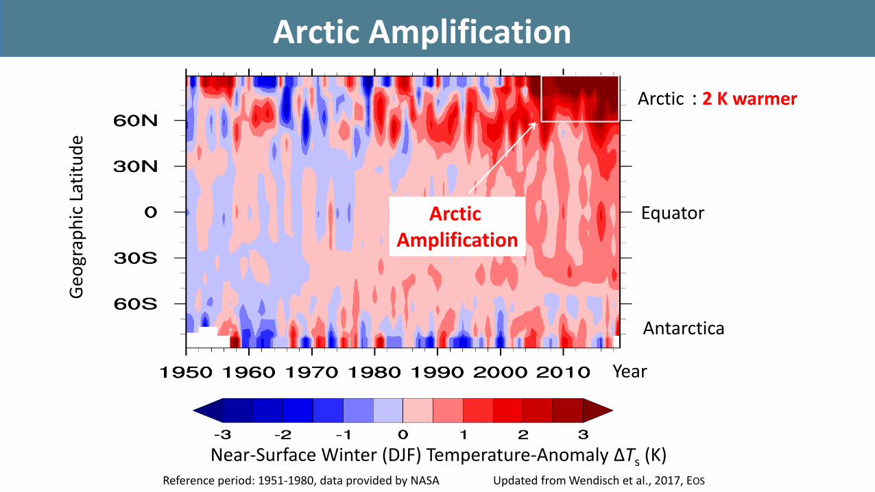
Arctic Amplification

Arctic

Equator

Antarctica

Reference period: 1951-1980, data provided by NASA Updated from Wendisch et al., 2017, EOS

Near-Surface Winter (DJF) Temperature-Anomaly ΔTs (K)

Arctic Amplification

: 2 K warmer

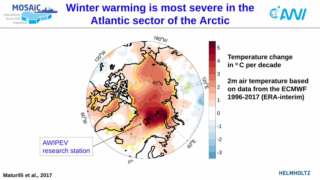
AWIPEV

research station

Winter warming is most severe in the

Atlantic sector of the Arctic

Maturilli et al., 2017

Temperature change

in o C per decade

2m air temperature based

on data from the ECMWF

1996-2017 (ERA-interim)

5

4

3

2

1

0

-1

-2

-3

Arctic Sea Ice Retreat from satellite data

40 % Loss

https://seaice.uni-bremen.de

https://seaice.uni-bremen.de/

Interplay of local, regional & global scales for Arctic Amplification

How are individual Arctic feedbacks

Atmospheric vertical stability

Surface heat fluxes

Low cloud response

Horizontal heat transports

Ocean heat uptake processes

Planetary waves & tropo-stratospheric coupling

quantitatively linked to hemispheric changes in

Teleconnection patterns

Weather regimes & extremes

Storm paths?

Dethloff et al., NYAS, 2019

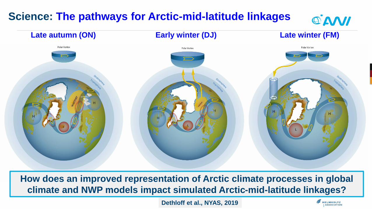
Late autumn (ON) Late winter (FM)Early winter (DJ)

How does an improved representation of Arctic climate processes in global

climate and NWP models impact simulated Arctic-mid-latitude linkages?

Science: The pathways for Arctic-mid-latitude linkages

Outline

MOSAiC Motivation

Earlier attempts

Logistics

Coupled system

Atmosphere

Ocean-Sea Ice


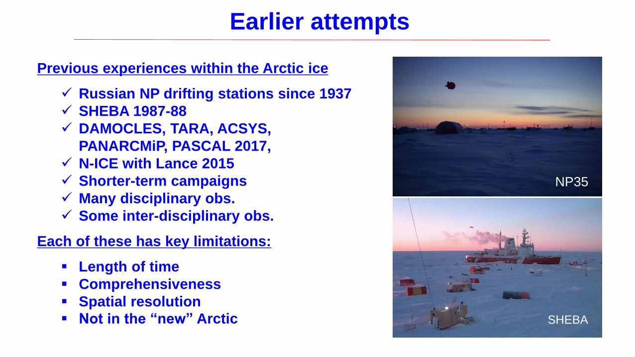
Previous experiences within the Arctic ice

Russian NP drifting stations since 1937

SHEBA 1987-88

DAMOCLES, TARA, ACSYS,

PANARCMiP, PASCAL 2017,

N-ICE with Lance 2015

Shorter-term campaigns

Many disciplinary obs.

Some inter-disciplinary obs.

Each of these has key limitations:

Length of time

Comprehensiveness

Spatial resolution

Not in the “new” Arctic

Russian drifting station

SHEBA

Earlier attempts

NP35

Drift-Station NP 35 Sept. 2007- April 2008

as part of the International Polar Year 2007-2008

Record minimum (Sep. 2007)

Arctic sea ice cover

NP 35 Route

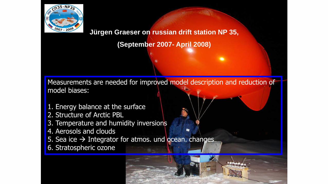
Jürgen Graeser on russian drift station NP 35,

(September 2007- April 2008)

Measurements are needed for improved model description and reduction of model biases:

1. Energy balance at the surface 2. Structure of Arctic PBL3. Temperature and humidity inversions4. Aerosols and clouds5. Sea ice Integrator for atmos. und ocean. changes

6. Stratospheric ozone

Need for Improved ModelsWeather, Climate, Sea-ice, Biogeochemistry & Ecosystems

Lack of data in the Arctic atmosphere over the ocean

Major deficiencies in Arctic process understanding

Clouds, boundary layer turbulence, winds, surface fluxes …

Need to focus on “processes, feedbacks and coupling”

Require physical representation of the changing new Arctic

SHEBA 1997-1998 in the old Arctic:

Surface Heat Budget of the Arctic Ocean

SHEBA trajectory Beaufort Sea

Validation and improvement of RCMs:

NP 35 Sept. 2007-July 2008 IPY

ARCMIP

Arctic Regional Climate Model Intercomparison

RCM biases 10-25 W/m2 against SHEBA radiative

fluxes especially under clouds.

Implications for sea-ice concentrations.

Bias of 10 W/m2 equivalent to energy of melting

about 1 m of ice.

Outline

MOSAiC Motivation

Earlier attempts

Logistics

Coupled system

Atmosphere

Ocean-Sea Ice


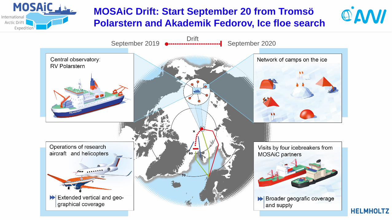
DriftSeptember 2020September 2019

MOSAiC Drift: Start September 20 from Tromsö

Polarstern and Akademik Fedorov, Ice floe search

DriftSeptember 2020September 2019

Fuel depots for emergency operations

Fuel depots (200 tons)

for emergency helicopter

operations on Severnaya

Zemlya (August 2019)

AK Treshnikov

Helicopter base

Longyearbyen

Expedition timeline

Start: 20 September 2019 Tromsoe End: 14 October2020

Mid DecemberKapitan Dranitzyn

Mid June – mid July2 x Oden

Mid AugustXuelong orXuelong II

Mid FebruaryKapitan Dranitzyn

Mid AprilAntonov AN-74

Ice runway3x AN-74

Until mid OctAkademik

Fedorov

2

MOSAiCInternational expedition and example for cooperation in the Arctic

• 20 Sep 20:00 CET: Polarstern departs Tromso21:00 CET: Akademik Fedorov departs Tromso

Ships travel together ~14kn (in open water)

• 1 Oct: At target area ~120-130 E, ~85 N. Start searching floe• 6 Oct: At floe, transfer of equipment and personel between

Polarstern and Fedorov• 7-12 Oct: Fedorov sets up Distributed Network of buoys, • Polarstern starts to set up central observatory• 13-15 Oct: Transfer of fuel Fedorov-Polarstern• 16-30 Oct: Fedorov goes back to Tromso• latest 20 Oct: Start of standard observations at central obs.

Timeline first phaseall dates will change based on ice conditions

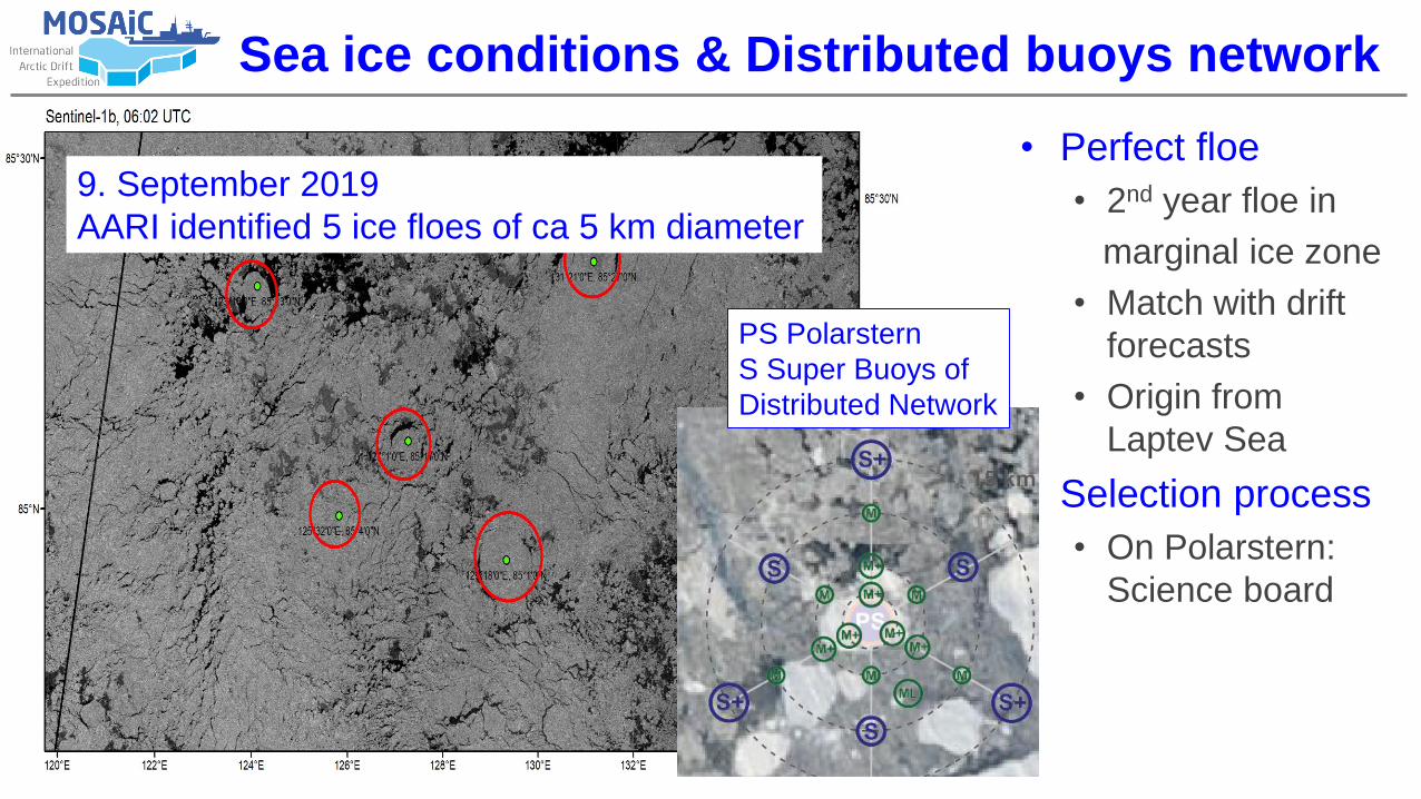
• Perfect floe

• 2nd year floe in

marginal ice zone

• Match with drift

forecasts

• Origin from

Laptev Sea

• Selection process

• On Polarstern:

Science board

Sea ice conditions & Distributed buoys network

PS Polarstern

S Super Buoys of

Distributed Network

9. September 2019

AARI identified 5 ice floes of ca 5 km diameter

Sea ice observatory with runway

Met, Ocean, ECO, BGC,

ICE sites - close to RV

Polarstern, depends on

snow and ice conditions

Runway specification:

• UTAir (length-width-thick):

1400 m / 35 m / 1 m

(reduced payload)

• KBAL (length-width-thick):

1200 m / 28 m / 1 m

• Distance from ship

at least 1 – 2 km

© Marcel Nicolaus, AWI

Daily schedule

Weather forecast by DWD

Peter Gege PASCAL June 2017

German Meteorological Service – Marine Met Office MOSAiC Workshop, Potsdam 2019

Weather forecast by DWD Product examples

Flight weather report Maritime weather report

Outline

MOSAiC Motivation

Earlier attempts

Logistics

Coupled system

Atmosphere

Ocean-Sea Ice


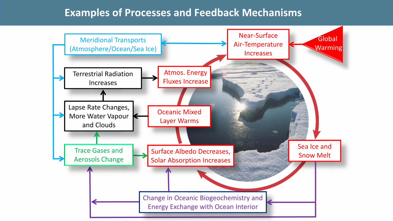
Sea Ice andSnow Melt

Oceanic Mixed Layer Warms

Atmos. EnergyFluxes Increase

Terrestrial Radiation Increases

Lapse Rate Changes, More Water Vapour

and Clouds

Meridional Transports(Atmosphere/Ocean/Sea Ice)

Near-Surface Air-Temperature

Increases

Global Warming

Surface Albedo Decreases,Solar Absorption Increases

Trace Gases andAerosols Change

Examples of Processes and Feedback Mechanisms

Change in Oceanic Biogeochemistry and Energy Exchange with Ocean Interior

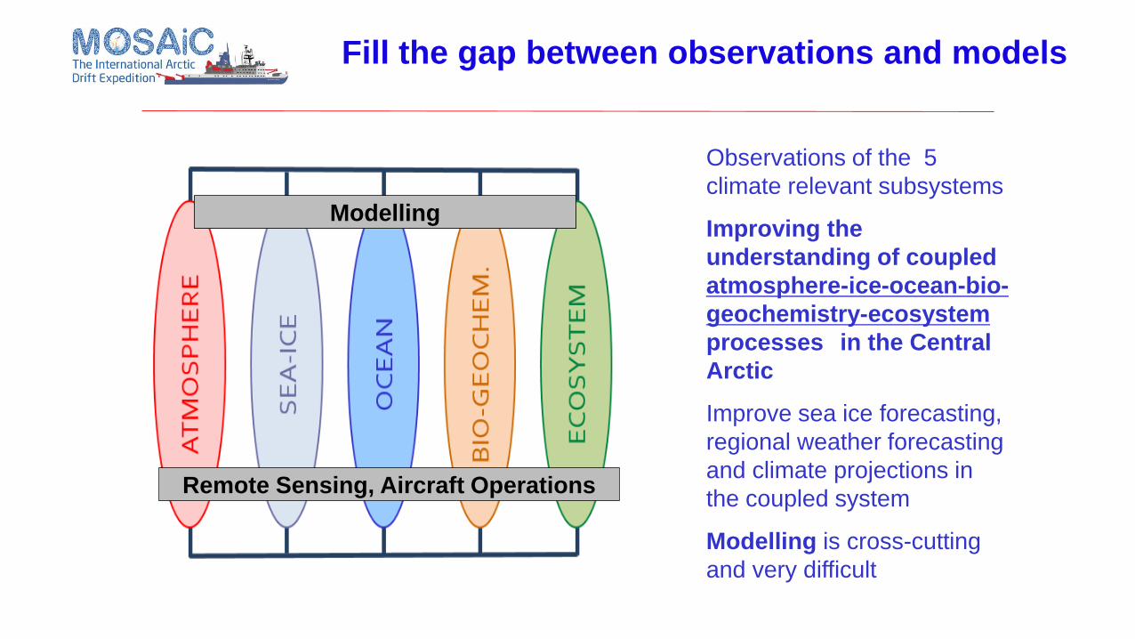
Observations of the 5

climate relevant subsystems

Improving the

understanding of coupled

atmosphere-ice-ocean-bio-

geochemistry-ecosystem

processes in the Central

Arctic

Improve sea ice forecasting,

regional weather forecasting

and climate projections in

the coupled system

Modelling is cross-cutting

and very difficult

Remote Sensing, Aircraft Operations

ModellingModelling

Fill the gap between observations and models

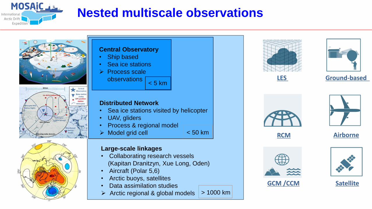
Large-scale linkages

• Collaborating research vessels

(Kapitan Dranitzyn, Xue Long, Oden)

• Aircraft (Polar 5,6)

• Arctic buoys, satellites

• Data assimilation studies

Arctic regional & global models > 1000 km

Distributed Network

• Sea ice stations visited by helicopter

• UAV, gliders

• Process & regional model

Model grid cell < 50 km

< 5 km

Central Observatory

• Ship based

• Sea ice stations

Process scale

observations

Airborne

Satellite

Ground-basedLES

RCM

GCM /CCM

Nested multiscale observations

Modelling hierarchy and data assimilation for upscaling

• Operational weather forecasts: DWD, ECMWF

• Operational sea ice forecasts: AARI

• Large-eddy simulations

• Single column models

• Regional models

Atmosphere

Ocean-Sea Ice

Coupled A-O-I

• Data assimilation in regional BGC models

• Data assimilation in global models

• Improving sub-grid scale parameterizations

• Intensive Observing Period February-March 2020

for YOPP

Radiosondes over land and ships

llustration of the ICON model family used within (AC)3 representing the model strategy and the coverage from global to local scales. Global modelling includes ICON:

Icosahedral non–hydrostatic atmospheric general circulation model, ICON–HAM: Coupled climate–aerosol model, ICON–SWIFT: Coupled climate–ozone

model, and ICON–O: Icosahedral global ocean model. Regional modelling applies ICON as a nested Limited Area Model (LAM), while on the process level simulations with

the ICON-LEM (Large-Eddy Model) will be performed. These ICON family members will be for the irst time extensively tested and utilised in the Arctic region.

Process understanding, sub-grid scale parameterisation development for different synoptical conditions

Large-and meso-scale forcing as function of model complexity

ICON strategy for upscaling

Improved sub-gridscale parameterisations and data assimilation

GCM RCM LES

Extra Arctic radiosonde observations with RV Mirai and Polarstern

Improvements of weather and sea-ice forecasts over Northern Sea Route

high waves, strong winds, icing due Arctic cyclones

Better understanding of Arctic-mid latitudes linkage

extreme events over Eurasia (e.g. severe winter)

Data sparse areaExtra

Observations

Data

assimilation

Better predictions YOPP

ARCROSE: Arctic Research Collaboration

for Radiosonde Observing System Experiment

Ongoing Japan-Germany Arctic Predictability study

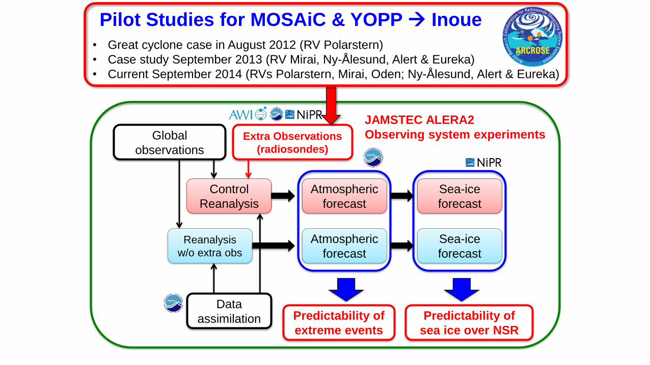
Extra Observations

(radiosondes)

Data

assimilation

Reanalysis

w/o extra obs

Control

Reanalysis

Global

observations

Atmospheric

forecast

Sea-ice

forecast

Atmospheric

forecast

Sea-ice

forecast

Predictability of

extreme events

Predictability of

sea ice over NSR

Pilot Studies for MOSAiC & YOPP Inoue

• Great cyclone case in August 2012 (RV Polarstern)

• Case study September 2013 (RV Mirai, Ny-Ålesund, Alert & Eureka)

• Current September 2014 (RVs Polarstern, Mirai, Oden; Ny-Ålesund, Alert & Eureka)

JAMSTEC ALERA2

Observing system experiments

Outline

Logistical preparations

Earlier attempts

MOSAiC motivation

Coupled system

Atmosphere

Ocean-Sea Ice


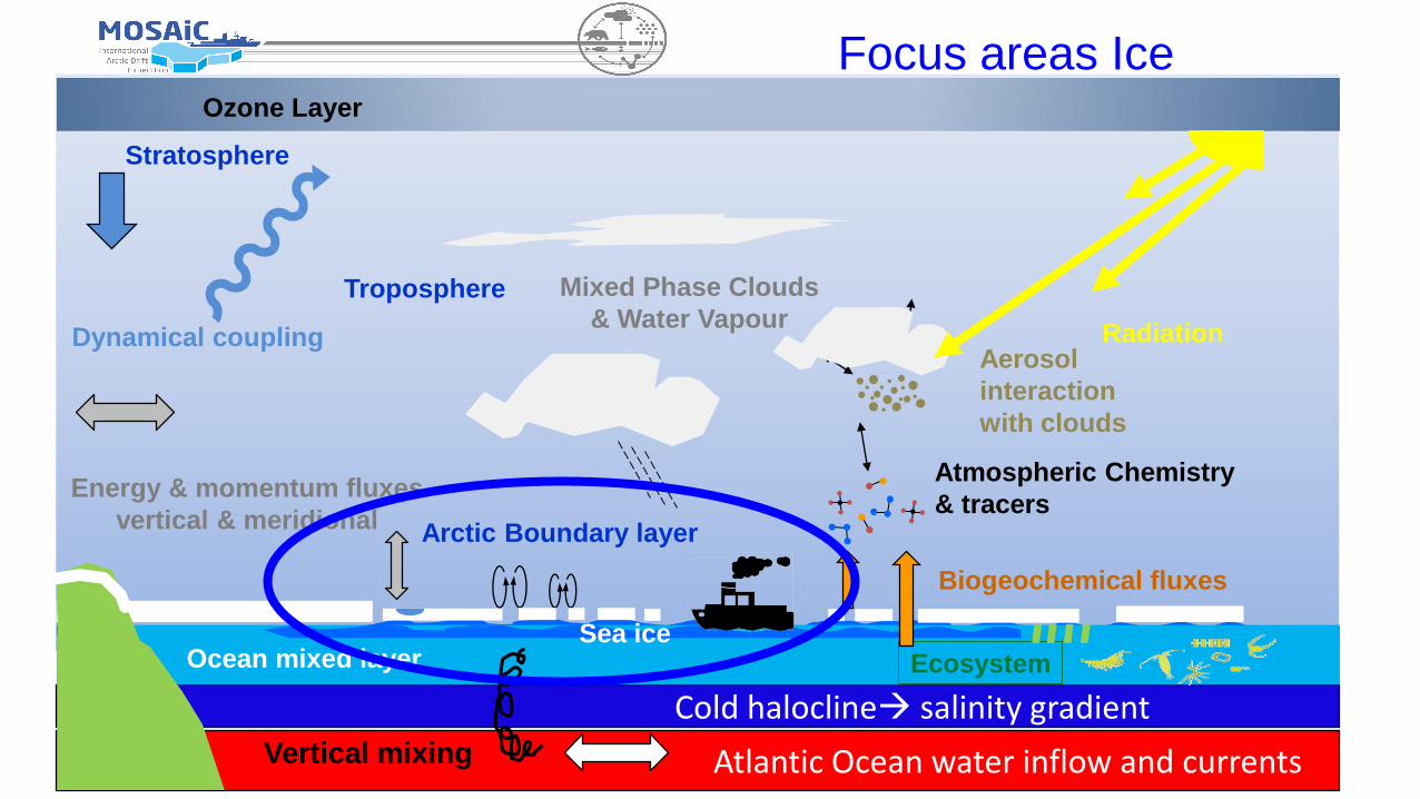
Atlantic Ocean water inflow and currents

Focus areas MOSAiC

Aerosol

interaction

with clouds

Ozone Layer

Dynamical coupling

Arctic Boundary layer

Troposphere

Stratosphere

Mixed Phase Clouds

& Water Vapour

Sea iceOcean mixed layer Ecosystem

Energy & momentum fluxes

vertical & meridional

Radiation

Biogeochemical fluxes

Atmospheric Chemistry

& tracers

Vertical mixing

Cold halocline salinity gradient



Focus areas Atmosphere

Aerosol

interaction

with clouds

Ozone Layer

Dynamical coupling


Troposphere

Stratosphere

Mixed Phase Clouds

& Water Vapour




Radiation



& tracers

Vertical mixing

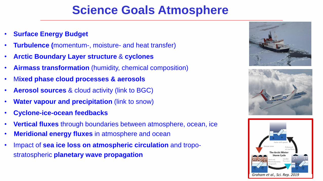
Science Goals Atmosphere

• Surface Energy Budget

• Turbulence (momentum-, moisture- and heat transfer)

• Arctic Boundary Layer structure & cyclones

• Airmass transformation (humidity, chemical composition)

• Mixed phase cloud processes & aerosols

• Aerosol sources & cloud activity (link to BGC)

• Water vapour and precipitation (link to snow)

• Cyclone-ice-ocean feedbacks

• Vertical fluxes through boundaries between atmosphere, ocean, ice

• Meridional energy fluxes in atmosphere and ocean

• Impact of sea ice loss on atmospheric circulation and tropo-

stratospheric planetary wave propagation

Graham et al., Sci. Rep. 2019

Arctic sea ice anomalies “Low-High”

AFES Atmos GCM

Isolated sea ice impact

NICE-CNTL Differences

ERA-Interim

LOW-HIGH

SON DJF

Seasonal sea ice concentration (%) maps – Difference betw. Low and High ice conditions

• Very similar distribution of concentration anomalies

HIGH ice (1979/80-1999/00)

Low ice (2000/01-2013/14)

CNTL: High ice conditions as

observed from 1979-1983

NICE: Low ice conditions as

observed from 2005-2009

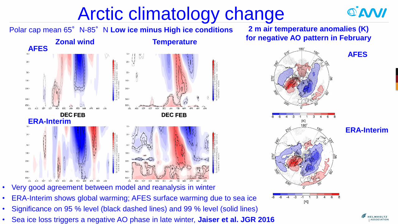
Arctic climatology change

Zonal wind Temperature

Polar cap mean 65°N-85°N Low ice minus High ice conditions

AFES

ERA-Interim

• Very good agreement between model and reanalysis in winter

• ERA-Interim shows global warming; AFES surface warming due to sea ice

• Significance on 95 % level (black dashed lines) and 99 % level (solid lines)

• Sea ice loss triggers a negative AO phase in late winter, Jaiser et al. JGR 2016

DEC FEBDEC FEB

2 m air temperature anomalies (K)

for negative AO pattern in February

ERA-Interim

AFES

Structure DFG Transregio TR 172, AC3 Arctic Amplification, Wendisch et al. 2019

A: Fluxes in the Arctic

Boundary Layer

C: Ocean, Atmosphere &

Sea Ice Interaction

C01: Surface heterogeniety & flux

observations

C03: Atmospheric composition &

ocean colour feedback

C04: Ocean-sea ice processes

D: Atmospheric

Circulation & Transport

D01: Atmospheric large-scale

dynamics

D02: Aerosol-cloud interactions

D03: Atmosphere-ice-ocean

interactions

D04: Ocean heat transport & regional processes

B: Clouds, Aerosols &

Water Vapour

B01: Changes of TOA reflectance

& clouds

B02: Aerosol & surface spectral

reflectance

B03: Mixed-phase cloud

observations

B04: Aerosols & cloud formation

B05: Water vapour trends

B07: Sea ice leads & clouds

E: Integration &

Synthesis

E01: Lapse rate feedback

E02: Ny-Ålesund column

E03: Mixed-phase cloud

processessE04: Precipitation & snowfall

A01: Surface radiation fluxes

A02: Local energy budget profiles

A03: Areal energy flux profiles

UNI Leipzig,

UNI Bremen,

UNI Köln,

AWI Bremerhaven,

AWI Potsdam,

TROPOS Leipzig

Outline


Earlier attempts

MOSAiC motivation

Coupled system

Atmosphere

Ocean-Sea Ice




Focus areas Ice

Aerosol

interaction

with clouds

Ozone Layer

Dynamical coupling


Troposphere

Stratosphere

Mixed Phase Clouds

& Water Vapour




Radiation



& tracers

Vertical mixing

Focus on different processes during the year

Oct Nov Dec Jan Feb Mar Apr May Jun Jul Aug Sep

Freeze-up &

Ice Growth

Sea ice dynamics

Snow properties

Sea ice optics &

Melt processes

• Formation of young ice

• Ice Drift pattern

• Deformation processes

• Melting from above and below

• Snow on ice and chemistry

• Melt ponds and polynyas

• Vertical fluxes through the ice

• Coupling to ecosystem

Cold halocline salinity


Focus areas Ocean

Aerosol

interaction

with clouds

Ozone Layer

Dynamical coupling


Troposphere

Stratosphere

Mixed Phase Clouds

& Water Vapour




Radiation



& tracers

Vertical mixing

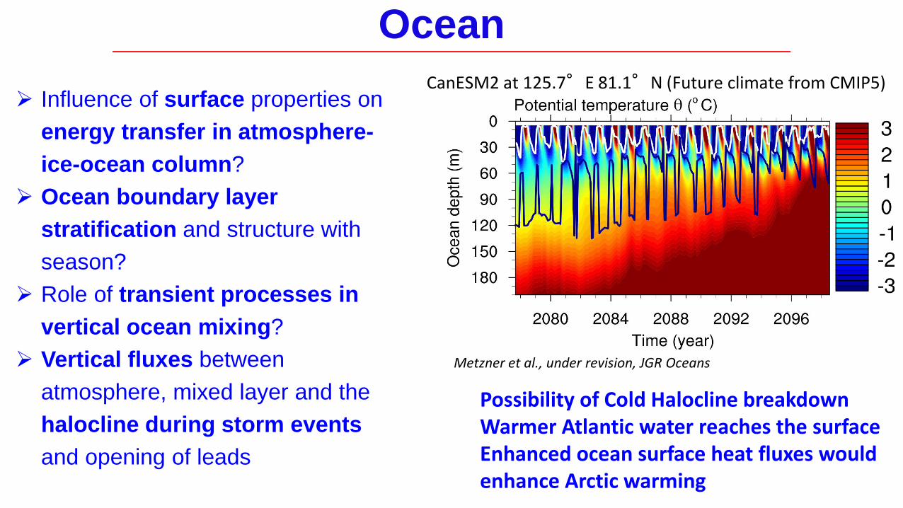
Ocean

Influence of surface properties on

energy transfer in atmosphere-

ice-ocean column?

Ocean boundary layer

stratification and structure with

season?

Role of transient processes in

vertical ocean mixing?

Vertical fluxes between

atmosphere, mixed layer and the

halocline during storm events

and opening of leads

Possibility of Cold Halocline breakdownWarmer Atlantic water reaches the surfaceEnhanced ocean surface heat fluxes would enhance Arctic warming

CanESM2 at 125.7°E 81.1°N (Future climate from CMIP5)

Metzner et al., under revision, JGR Oceans

Drifting Buoys

Gra

ph

ic:

Alf

red

-Weg

ener

-In

stit

ute

/FR

AM

/ Sa

bin

e Lü

del

ing

Multidisciplinary Ice-based Distributed Observatory (MIDO)

Buoy „array systems“ Distributed network

• Array: instruments on central floe and 25 km

• Multi-disciplinary observations

• Critical element of YOPP

Outline


Earlier attempts

MOSAiC motivation

Coupled system

Atmosphere

Ocean-Sea Ice


Cold halocline salinity


Focus areas BGC and ECO

Aerosol

interaction

with clouds

Ozone Layer

Dynamical coupling


Troposphere

Stratosphere

Mixed Phase Clouds

& Water Vapour


Energy & momentum Fluxes


Radiation



& tracers

Vertical mixing

• What are main biogeochemical

processes controlling

Mercury Hg

Volatile Organic Compounds (VOC)

Dimethylsulphide (DMS) cycling in

Arctic Ocean?

Annual cycle over the Arctic Ocean

• How are cycles of Mercury, halogens

(bromine and iodine), Ozone, VOCs,

and Dimethylsulphide connected in

ocean, ice, and atmosphere?

• Impact of DMS on Ice nucleation

and Cloud condensation particles?

• Connection to ocean biology?

Biogeochemical processes

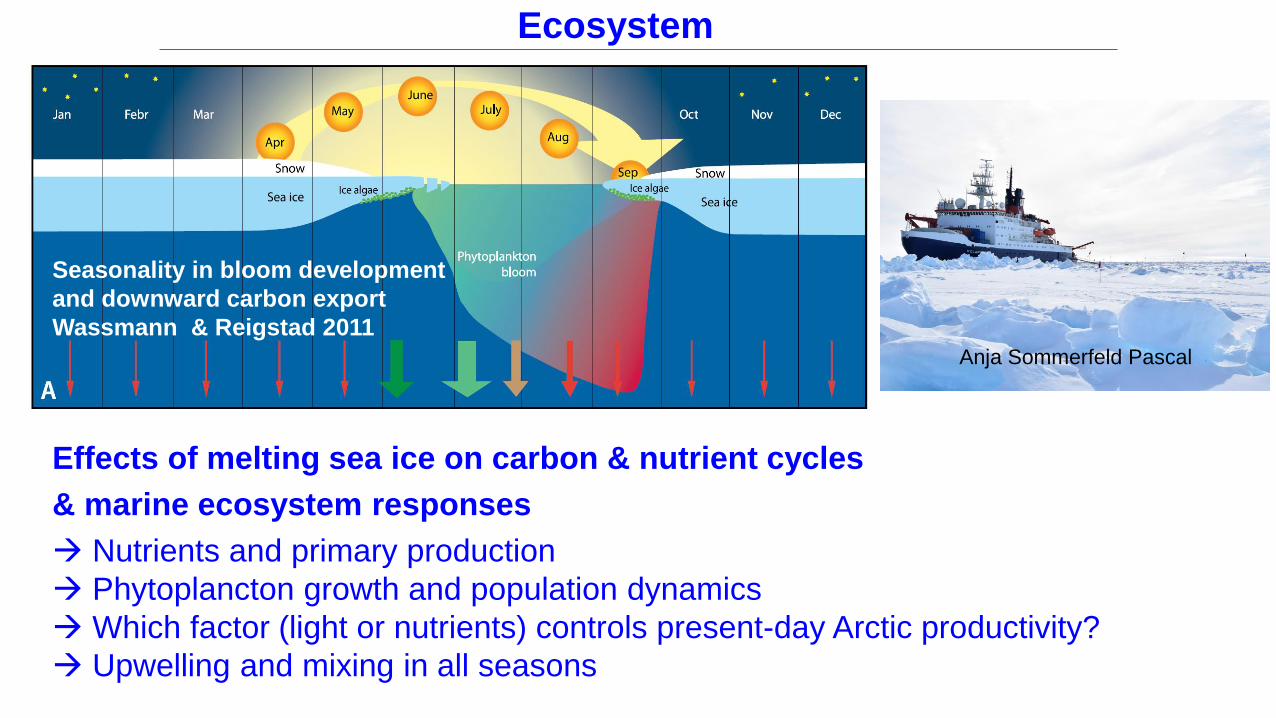
Effects of melting sea ice on carbon & nutrient cycles

& marine ecosystem responses

Nutrients and primary production

Phytoplancton growth and population dynamics

Which factor (light or nutrients) controls present-day Arctic productivity?

Upwelling and mixing in all seasons

Ecosystem

Seasonality in bloom development

and downward carbon export

Wassmann & Reigstad 2011

Anja Sommerfeld Pascal

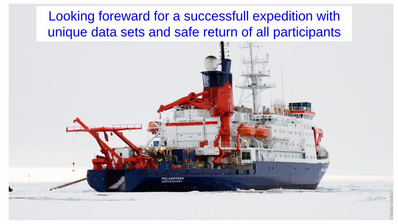
Looking foreward for a successfull expedition with

unique data sets and safe return of all participants

das mosaic driftexperiment dwd offenbach 18.09.2019 markus ... · das mosaic driftexperiment dwd...

Documents