data analysis and interpretationshodhganga.inflibnet.ac.in/bitstream/10603/40784/9/09_chapter...
TRANSCRIPT

Data analysis
And
Interpretation

Data Analysis an Interpretation
155
CHAPTER- 3
Data Analysis and Interpretation
In the current chapter various factors related with job satisfaction of employees
specifically to higher education sector are analyzed through the framed set of hypothesis with the
vision to analyze Employee Job Satisfaction in public and private universities of Rajasthan. It
elaborates the significance of various statistical tests which are applied in study. The chapter
briefly describes the primary points of satisfaction of various employees in higher education
related with their job. The current chapter also enlightens the interview of selected faculty
members of university under study, to analyze the factors responsible for job satisfaction in their
university. To strengthen the logics evolved in the research and to justify the hypothesis related
with the current study, various supporting data is also discussed in the chapter.
The survey was conducted among employees (100 no’s each) of three private sector
universities of Rajasthan (Viz Jaipur National University, Jaipur, Suresh Gyan Vihar University,
Jaipur, and Banasthali University, Niwai, Jaipur) and three public sector universities of
Rajasthan (Viz Rajasthan University, Jaipur, Mohanlal Sukhadia University, Udaipur, Jai
Narayan Vyas University, Jodhpur).Before conducting the survey the researcher introduced
himself and informed the faculties that their participation is absolutely anonymous, voluntary,
and confidential and gave assurance that they could ask questions if they faced with any
difficulty. All the two types of University faculties were also with asked some Interview
scheduled questions and their views on the topics were noted.

Data Analysis an Interpretation
156
3.1 TOOLS FOR DATA ANALYSIS
• Description Of Tools-
• Questionnaire
• Intensive Interviews
The main techniques used in this study was to collect first hand data that is primary data,
using the questionnaire containing questions both open ended & close ended. One set of
questionnaire was formed for two different categories of Universities of Rajasthan.(viz Public
and Private sector University). The questionnaire was divided into several parts {Questionnaire
is attached as Annexure A at last of the thesis}
a) First part Section A consisted of Socio Dynamic Information i.e primary information
regarding Respondent’s Name, Age, Sex, Designation, Experience etc.
b) The second part of the questionnaire i.e Section B deals with the segment of career
advancement of faculty and their correlation with Job satisfaction
c) Section C constitutes the questions related to Job reward among faculty and their
correlation with Employ Job satisfaction
d) Next part consists of Section D which deals with views of faculties related with work life
balance.
e) The another part section E of questionnaire deals with the intensive views of employees of
various universities on facts related with Administration / Management
f) Next part consists of Section F which deals with views of faculties related with Infrastructure
and Technology.

Data Analysis an Interpretation
157
g) The last section G of questionnaire deals with certain miscellaneous questions related with
the aim of the research.
Overall there are 37 questions which are divided into above mentioned sections and the
comparative analysis of these sections on 300 respondents of private university and 300
respondents of public university of Rajasthan is analyzed in the current chapter.
3.2 TOOLS FOR HYPOTHESIS TESTING
Hypothesis testing is the use of statistics to determine the probability that a given
hypothesis is true or not. The usual process of hypothesis testing consists of four steps.
1. Formulate the null hypothesis Ho (commonly, that the observations are the result of pure
chance) The employees in the Public sector have higher level of satisfaction as compared to
the Private sector. And the alternative hypothesis Ha (commonly, that the observations show a
real effect combined with a component of chance variation) i.e. The employees in the Private
sector have higher level of satisfaction as compared to the Public sector.
2. Identify a statistical test that can be used to evaluate the truth of the null hypothesis.
Certain secondary hypothesis framed to justify and favor the null (Primary hypothesis) as framed
above are:-
H2: The indicators of Job satisfaction like salaries, fringe benefits, social security, etc are more
favourable in Public sector.
H3: The quality of work-life balance is better in Public sector employees as compared to Private
sector employees.
Data Analysis an Interpretation
158
H4: Private sector employees have more exposure of working in various sectors such as
Administrative etc.
H5: Public sector jobs offer more stability.
H6: Sense of belongingness to the organization is more in Public sector employees as compared
to Private sector employees.
H7: Private sector employees gave better chances and facilities for higher education in the same
university
3. Compute the P-value, which is the probability that a test statistic at least as significant as the
one observed would be obtained assuming that the null hypothesis were true. The smaller the P-
value, the stronger the evidence against the null hypothesis.
4. Compare the p-value to an acceptable significance value alpha (sometimes called an alpha
value). If p<=alpha, that the observed effect is statistically significant, the null hypothesis is
ruled out, and the alternative hypothesis is valid.
For hypothesis testing the following statistical techniques are been used on the tabulated data.
The data collected from the questionnaire will be used to check the hypothesis. For hypothesis
testing the following statistical techniques are been used on the tabulated data.
• Students “t” test (Agarwal N.P; (2011)1
Hypothesis Among the most regularly utilized measurable centrality tests connected to little
information sets (populace's examples) is the arrangement of Student's tests. One of these tests is
utilized for the examination of two methods, which is ordinarily connected to numerous cases.

Data Analysis an Interpretation
159
Normal cases are:
Illustration 1: Comparison of investigative effects acquired with the same technique on
specimens A and B, to affirm if both examples hold the same rate of the measured dissect or not.
Illustration 2: Comparison of investigative effects acquired with two separate techniques
A and B on the same specimen, to affirm if both strategies give comparable logical outcomes or
not.
• General Aspects of Significance Tests (Ahuja Ram, 2001)2
The conclusion of these tests is the acknowledgement or dismissal of the invalid theory
(H0). The invalid speculation for the most part states that: "Any contrasts, errors, or suspiciously
distant outcomes are absolutely because of arbitrary and not precise slips". The elective theory
(Ha) states precisely the inverse.
The invalid theory for the previously stated samples is:
The methods are the same, i.e. in Example 1: both examples hold the same rate of the
examine; in Example 2: both strategies give the same investigative outcomes. The contrasts
watched (if any) are simply because of irregular failures.
The elective theory is: The methods are altogether diverse, i.e. in Example 1: each one specimen
holds an alternate rate of the diagnostic; in Example 2: the strategies give distinctive scientific
comes about (so no less than one system yields precise expository mistakes).
A wrong dismissal of H0 (in spite of the fact that it is accurate) constitutes a Type 1
failure, inasmuch as a mistaken acknowledgement of H0 (in spite of the fact that it is false)
constitutes a Type 2 lapse.
Data Analysis an Interpretation
160
All essentialness tests furnish comes about inside a predefined certainty level % (Cl%).
Certainty levels ordinarily utilized are 90%, 95% and 99%, with most common (anyhow in the
field of synthetic examination) the 95%.
A CL 95% implies that: in the event of dismissing Ho, we are 95% or more sure that we
made the best choice. As it were, we hazard a likelihood of close to (100-95)/100 = 0.05 for a
Type 1 blunder.
We can lessening or expansion the certainty level of a criticalness test, yet one need to
think about the accompanying pitfalls:
(a) By diminishing CL say to 90% (making therefore the dismissal of H0 less demanding)
the likelihood of Type 1 slip clearly builds.
(b) By expanding CL say to 99% (making therefore the dismissal of H0 harder) the
likelihood of Type 2 lapse increments. A CL 95% is by and large recognized as a reasonable
trade off between these two separate dangers.
• Student’s T-Test for the Comparison of Two Means (Ahuja Ram, 2006)3
This test (as depicted beneath) expects:
(a) An ordinary (Gaussian) dissemination for the populaces of the irregular lapses,
(b) There is no critical distinction between the standard deviations of both populace tests.
The two methods and the comparing standard deviations are computed by utilizing the
accompanying mathematical statements (na and nb are the amount of estimations in information
set An and information set B, individually):

Data Analysis an Interpretation
161
At that point, the pooled evaluation of standard deviation sab is computed: Finally, the
fact texp (exploratory t worth) is figured:
texp worth is contrasted and the basic (hypothetical) tth quality comparing to the given
level of opportunity N (in the present case N = na + nb - 2) and the certainty level picked. Tables
of basic t qualities might be found in any book of measurable dissection, and in addition in
numerous quantitative examination course books. Assuming that texp>tth then H0 is rejected else
H0 is accepted.
In the current research study students “t” test is been used as various tables to test the
hypothesis.
• ANOVA (Analysis Of Variance)
ANOVA, generally called a F test, is about related to the t test. The noteworthy
difference is that, where the t test measures the qualification between the system for two totals,
an ANOVA tests the differentiation between the strategy for two or more get-togethers.
A limited ANOVA, or a singular component ANOVA, tests differentiates between get-
togethers that are recently masterminded on one free variable. You can in like manner use
different self-governing variables and test for participations using factorial ANOVA (see
underneath). The playing purpose of using ANOVA rather than different t-tests is that it
decreases the probability of a sort I pass. Making diverse examinations raises the likelihood of
finding something by chance—creation a sort I oversight. (Allen Mike , 2008)4 how about we
use socioeconomic status (SES) as an outline. I have 8 levels of SES and I have to check if any
of the eight accumulations are not exactly the same as each one in turn on their ordinary

Data Analysis an Interpretation
162
fulfillment. To complexity the total of the strategies with each one in turn, you may need to run
28 t tests. On the off chance that your alpha is arranged at .05 for every one test, times 28 tests,
the new p is 1.4—you are essentially ensured of making a sort I botch. Consequently, you over
every one of the previously stated 28 tests you may run across some discriminating complexities
between social events, however there are likely on account of disappointment. An ANOVA
controls the generally pass by testing each one of the 8 systems against each other at once, so
your alpha stays at .05.
One potential drawback to an ANOVA is that you lose specificity: every one of the a F
tells you is that there is an imperative qualification between congregations, not which social
affairs are inside and out not the same as each one in turn. To test for this, you use a post-hoc
examination to find where the differences are – which social affairs are inside and out
exceptional in connection to each other and which are definitely not.
ANOVAs is receptive for both parametric (score data) and non-parametric
(ranking/ordering) data.
Sorts OF ANOVA
• One-Way Between Groups (Ambastha, C.k.,2001)5
There is emerge collecting (last audit) which you are using to portray the social events.
This is the slightest complex version of ANOVA. This kind of ANOVA can moreover be used to
remain up in correlation variables between assorted social affairs - excercise execution from
different concessions.

Data Analysis an Interpretation
163
• One-Way Repeated Measures
A confined repeated measures ANOVA is used when you have a singular get together on
which you have measured something several times. You may use one-way reiterated measures
ANOVA to check if researcher execution on the test changed after some time.
• Two-Way Between Groups
A two-way between get-togethers ANOVA is used to look at complex groupings. Each of
the rule effects are confined tests. The correspondence effect is fundamentally asking "is there
any huge refinement in execution when you take last survey and overseas/local acting together".
• Two-Way Repeated Measures
This type of ANOVA direct use the reiterated measures structure and fuses an association
sway.
• Non-Parametric And Parametric
Anova is approachable for score or between time data as parametric ANOVA. This is the
kind of ANOVA you do from the standard menu choices in a true cluster. The non-parametric
variant is typically found under the heading "Nonparametric test". It is used when you have rank
or data.
Data Analysis an Interpretation
164
• Available Software (Essa, E. L,1987)6
(a) SPSS: - The ANOVA routines in SPSS are OK for simple one-way analyses. Anything more
complicated gets difficult. All statistical packages (SAS, Minitab etc.) provide for ANOVA.
(b) Excel:-Excel allows you to ANOVA from the Data Analysis Add-on. The instructions are
not good.
In the current research design two way ANOVA is been applied and values are interpreted
with the help of F test table as well as SPSS software.
• Chi-Square Test (A Goodness Of Fit)
Theory tests may be performed on possibility tables with a specific end goal to choose
whether or not impacts are available. Impacts in a possibility table are characterized as
relationships between the line and segment variables; that is, are the levels of the column
variable differentially dispersed over levels of the section variables. Centrality in this theory test
implies that understanding of the unit frequencies is justified. Non-criticalness implies that any
contrasts in cell frequencies could be clarified by possibility. (Garg. N.l ; Sharma. S.g; Jain.r.k &
Pareek.g ; 2007)8
Theory tests on possibility tables are dependent upon a fact called Chi-square. The testing
dispersion of the Chi-squared fact will then be exhibited, gone before by a discourse of the
theory test.
In likelihood hypothesis and facts, the chi-squared appropriation (likewise chi-square or χ²-
circulation) with k degrees of flexibility is the dispersion of a total of the squares of k free
standard ordinary irregular variables. It is a standout amongst the most broadly utilized
likelihood circulations within inferential facts, e.g., in theory testing or in development of

Data Analysis an Interpretation
165
certainty interims. The point when there is a necessity to complexity it with the noncentral chi-
squared dispersion, this appropriation is now and again called the focal chi-squared
dissemination.
The chi-squared circulation is utilized as a part of the regular chi-squared tests for integrity of
fit of a watched dissemination to a hypothetical one, the freedom of two criteria of grouping of
qualitative information, and in trust interim estimation for a populace standard deviation of an
ordinary dispersion from an example standard deviation. Numerous other factual tests
additionally utilize this conveyance, for example Friedman's examination of change by ranks.
The chi-square test of noteworthiness is suitable as a device to figure out whether it is worth
the specialist's exertion to translate a possibility table. A huge consequence of this test implies
that the units of a possibility table ought to be translated. A non-huge test implies that no impacts
were uncovered and chance could demonstrate the watched contrasts in the units. Thus, an
elucidation of the unit frequencies is not functional. (Kothari C.R.; 2004)8
In the current research design Chi Square is been applied and values are interpreted
with the help of table as well as SPSS software.
Interpretation is essential as the useful users and utility of researchers findings lie in
proper interpretation. It is through interpretation that the researcher can well understand the
abstract principle that work beneath the findings.

Data Analysis an Interpretation
166
3.3 TESTING OF HYPOTHESIS
(i) Demographic details of respondents
Demographic study means study of both quantitative and qualitative aspects of selected
human population. Quantitative aspects include composition, age, gender, size, and structure of
the population. Qualitative aspects are the research specific factors such as designation,
experience etc.
In the current research study Rajasthan state is chosen as the universe of study.
Employees of Public and Private sector universities were selected as the sample for the study.
Below tables and graphs shows the demographic details of faculties as the respondents.
Data Analysis an Interpretation
167
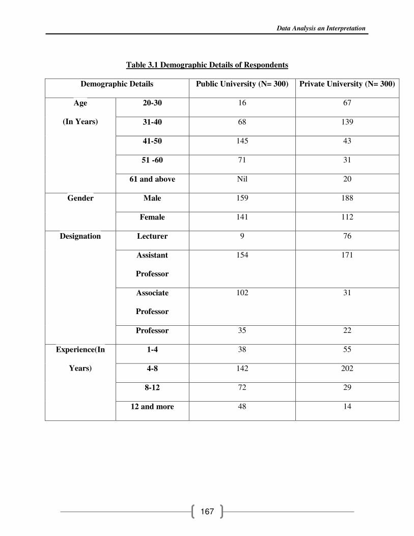
Table 3.1 Demographic Details of Respondents
Demographic Details Public University (N= 300) Private University (N= 300)
20-30 16 67
31-40 68 139
41-50 145 43
51 -60 71 31
Age
(In Years)
61 and above Nil 20
Male 159 188 Gender
Female 141 112
Lecturer 9 76
Assistant
Professor
154 171
Associate
Professor
102 31
Designation
Professor 35 22
1-4 38 55
4-8 142 202
8-12 72 29
Experience(In
Years)
12 and more 48 14
Data Analysis an Interpretation
168
Chart 3.1 (a &b) Age group of Respondents
Chart 3.1 (c & d) Age group of Respondents
Chart 3.1 (e & f) Designation of Respondents
Chart 3.1 (g & h) Experience of Respondents

Data Analysis an Interpretation
169
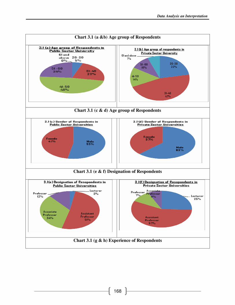
It is evident from the above demographic details of respondents that research had tried to
cover a broad demographic profile of faulty as respondents. As in the current study the total
sample size is n=600; (100 each of three public sector and three private sector universities). The
age group of 31-40 is higher in Private universities ( 47%)whereas mostly faculties under study
from public universities are of age 40-50 years (48%).The above fact also directly contributes to
Data Analysis an Interpretation
170
the designation and experience section of faculties as respondents under study. As there are 57%
Assistant Professors in private universities and 51% in Public University. Whereas the lower age
group respondents are Lecturers in Private university i.e 25% but this segment is only 3% in
public university.
Experience level of various respondents as faculty in public and private universities also
significantly coincides with the facts to be studied in current study as the most faculty in private
university i.e 67% is 4 to 8 years experience only but consequently on the other part only 47% is
having the same experience. The level of job satisfaction of may also be indirectly correlated
with the experienced faculty in the university, and the hypothesis of the research Ho- The
employees in the Public sector have higher level of satisfaction as compared to the Private
sector. Can be assumed to be expected as the 12 years and more experienced faculty in public
sector is significantly higher (16%) than private university (5%). This data supports the central
hypothesis of research study.
Another important demographic parameter which makes the study highly reliably and
increases the acceptance region of research is that in study both male and female gender faculty
of both types of universities have equally contributed as respondents of the study.
(ii) Correlation of Career Advancement of Employee with Job Satisfaction:-
A better job is a significant part of human growth, is the process through which an
individual's work identification is established. It covers a person's entire life-time. Profession
growth starts with a individual's very first attention of the ways in which people earn an income,
carries on as he or she examines professions and eventually chooses what career to engage in,

Data Analysis an Interpretation
171
makes for it, is applicable for and gets a job and developments in it. It may, and probably will
consist of, modifying professions and tasks.
The improved significance of career progression possibilities could be linked to workers
sensation that they have perfected the required their present roles and therefore are looking for
more complicated roles within their companies. The increase in the significance of this part may
also be relevant to employees’ doubt about the economic system, making it more likely for them
to desire progression within their company rather than taking the risk of shifting to a new
company. As this part is constantly on the pattern up in significance, companies need to pay
attention to employees’ fulfillment level with career progression possibilities.
Therefore in current research study certain set of questions are laid down in section B of
the research questionnaire which are correlated with job satisfaction of employees and career
advancement.

Data Analysis an Interpretation
172
Figure 3.1 Relationship of Age and Career advancement with Employee Job satisfaction
Table 3.2 Respondents Opinion about Career Advancement and Job Satisfaction
Strongly agree Agree Disagree Strongly
Disagree
Q.
No
Question
Public
Univ
Private
Univ
Public
Univ
Private
Univ
Public
Univ
Private
Univ
Public
Univ
Private
Univ
Q1 Has your present job
performance provided
you good further career
Opportunities?
119 12 106 86 59 141 16 61
Q4 Do you foresee a career
in your current job
231 52 65 146 03 74 01 28
Q5 Does your university
provide your adequate
basis facilities?
22 66 209 81 62 117 07 36

Data Analysis an Interpretation
173
Above table and chart 3.2 elaborates the career advancement of faculty and its correlation
with job satisfaction. As it is sated above that any individual after attaining some experience
expects some career opportunities to strengthen his or her future profile. As Q1 stated in above
table states the relevance of respondent’s job with career advancement and it is unexpected to see
that only 12 out of 300 private university respondents strongly agree with the fact whereas 119
are on the other counterpart university respondents. The disagree percentage with the career
advancement fact is relatively very high nearly 50% (141 out of 300) of private university
compared to 30% (9 1) of public university.
Opinions of respondents to the question 4 which clearly states fact that doe the urrent
faculty foresee future in their current job, and the results states that 231 respondents i.e nearly
80% of public university employees are well satisfied with their job and foresee a brighter future
in current job but on other side the no of strongly agree respondents are only 12 i.e 4% of total
Data Analysis an Interpretation
174
who see a future in their job with private university. But the respondents who opted for disagree
component of this fact is nearly 50% in private university segment.
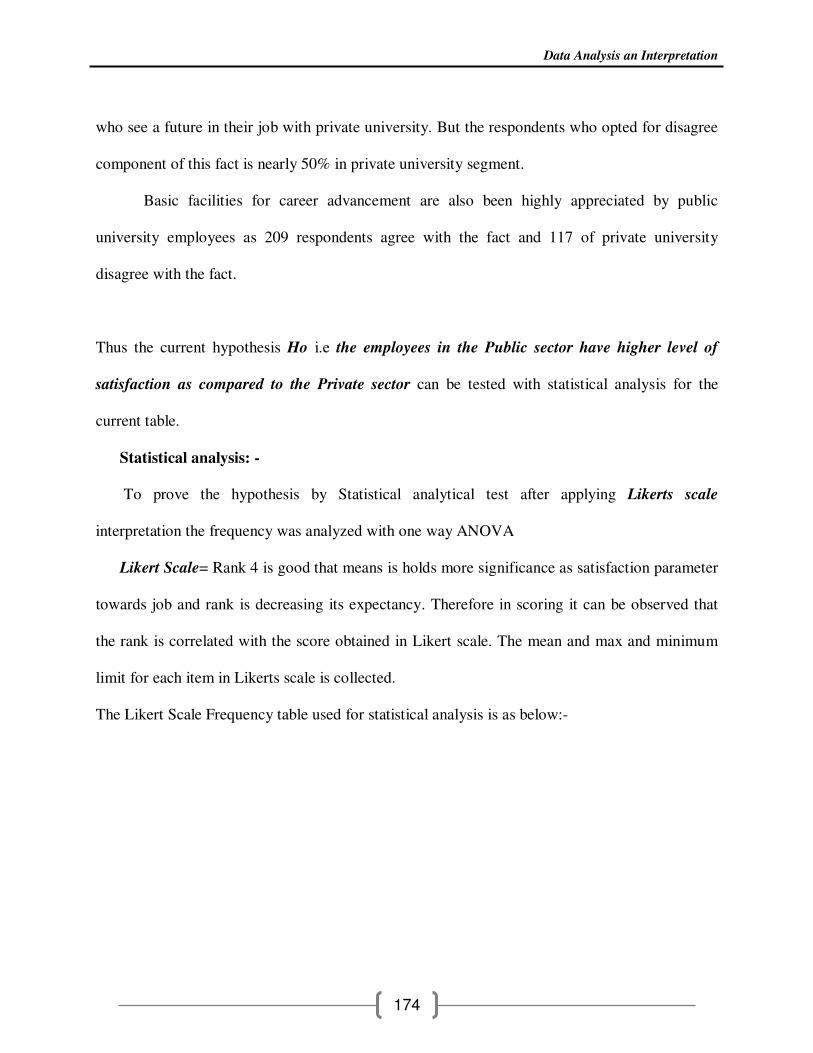
Basic facilities for career advancement are also been highly appreciated by public
university employees as 209 respondents agree with the fact and 117 of private university
disagree with the fact.
Thus the current hypothesis Ho i.e the employees in the Public sector have higher level of
satisfaction as compared to the Private sector can be tested with statistical analysis for the
current table.
Statistical analysis: -
To prove the hypothesis by Statistical analytical test after applying Likerts scale
interpretation the frequency was analyzed with one way ANOVA
Likert Scale= Rank 4 is good that means is holds more significance as satisfaction parameter
towards job and rank is decreasing its expectancy. Therefore in scoring it can be observed that
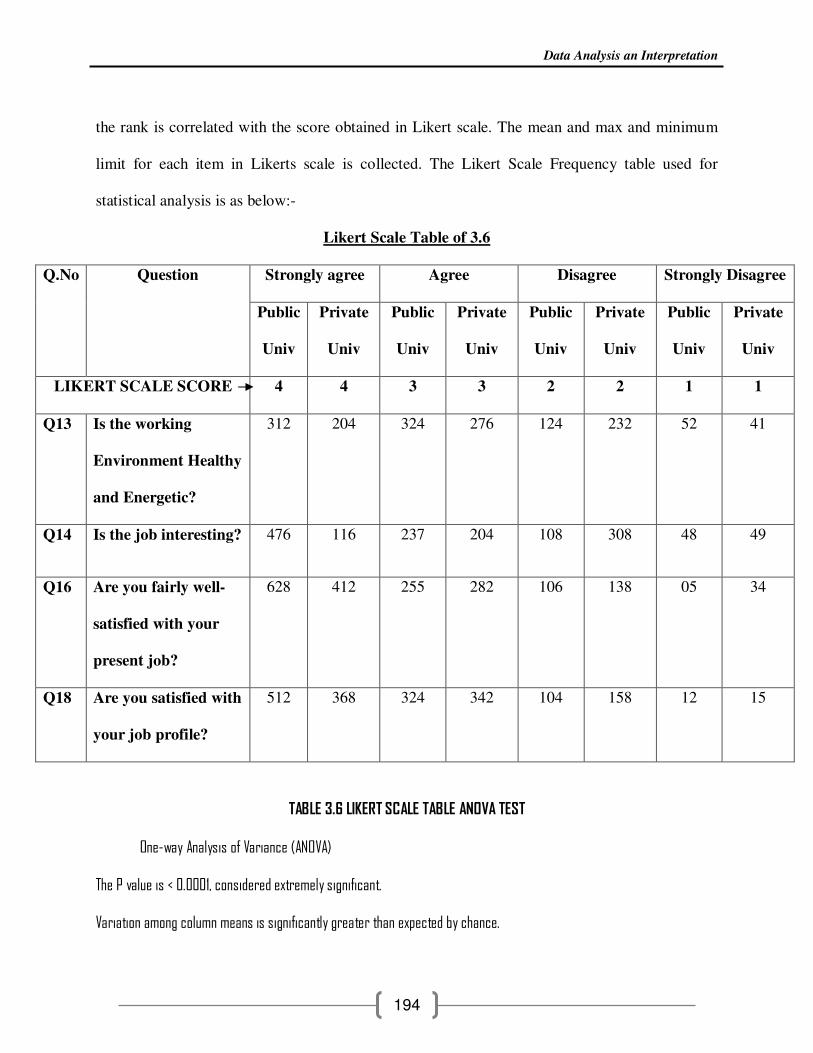
the rank is correlated with the score obtained in Likert scale. The mean and max and minimum
limit for each item in Likerts scale is collected.
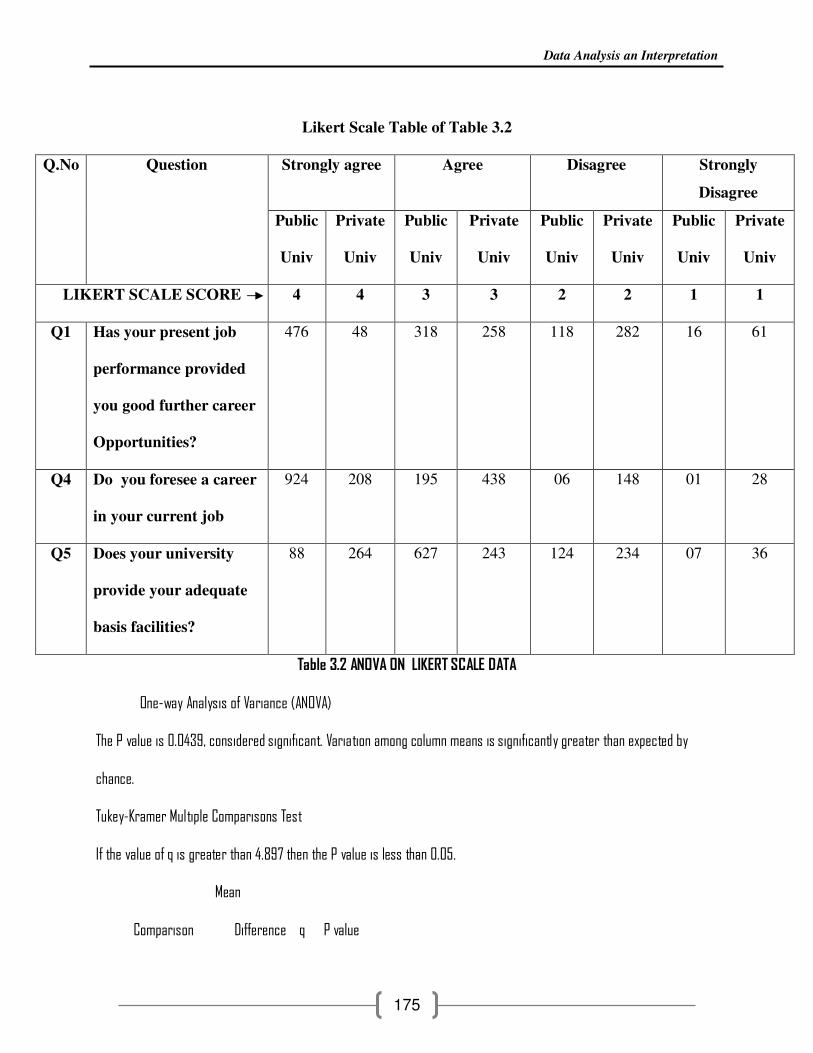
The Likert Scale Frequency table used for statistical analysis is as below:-
Data Analysis an Interpretation
175
Likert Scale Table of Table 3.2
Strongly agree Agree Disagree Strongly
Disagree
Q.No Question
Public
Univ
Private
Univ
Public
Univ
Private
Univ
Public
Univ
Private
Univ
Public
Univ
Private
Univ
LIKERT SCALE SCORE 4 4 3 3 2 2 1 1
Q1 Has your present job
performance provided
you good further career
Opportunities?
476 48 318 258 118 282 16 61
Q4 Do you foresee a career
in your current job
924 208 195 438 06 148 01 28
Q5 Does your university
provide your adequate
basis facilities?
88 264 627 243 124 234 07 36
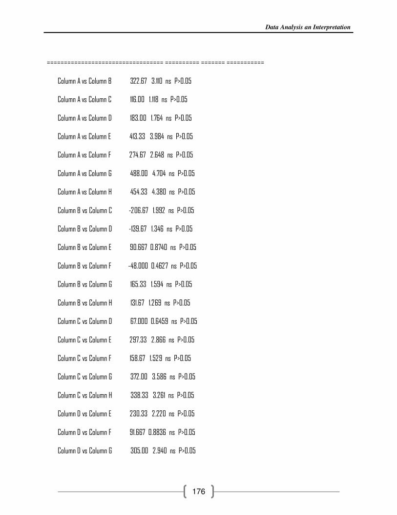
Table 3.2 ANOVA ON LIKERT SCALE DATA
One-way Analysis of Variance (ANOVA)
The P value is 0.0439, considered significant. Variation among column means is significantly greater than expected by
chance.
Tukey-Kramer Multiple Comparisons Test
If the value of q is greater than 4.897 then the P value is less than 0.05.
Mean
Comparison Difference q P value
Data Analysis an Interpretation
176
================================== ========== ======= ===========
Column A vs Column B 322.67 3.110 ns P>0.05
Column A vs Column C 116.00 1.118 ns P>0.05
Column A vs Column D 183.00 1.764 ns P>0.05
Column A vs Column E 413.33 3.984 ns P>0.05
Column A vs Column F 274.67 2.648 ns P>0.05
Column A vs Column G 488.00 4.704 ns P>0.05
Column A vs Column H 454.33 4.380 ns P>0.05
Column B vs Column C -206.67 1.992 ns P>0.05
Column B vs Column D -139.67 1.346 ns P>0.05
Column B vs Column E 90.667 0.8740 ns P>0.05
Column B vs Column F -48.000 0.4627 ns P>0.05
Column B vs Column G 165.33 1.594 ns P>0.05
Column B vs Column H 131.67 1.269 ns P>0.05
Column C vs Column D 67.000 0.6459 ns P>0.05
Column C vs Column E 297.33 2.866 ns P>0.05
Column C vs Column F 158.67 1.529 ns P>0.05
Column C vs Column G 372.00 3.586 ns P>0.05
Column C vs Column H 338.33 3.261 ns P>0.05
Column D vs Column E 230.33 2.220 ns P>0.05
Column D vs Column F 91.667 0.8836 ns P>0.05
Column D vs Column G 305.00 2.940 ns P>0.05

Data Analysis an Interpretation
177
Column D vs Column H 271.33 2.616 ns P>0.05
Column E vs Column F -138.67 1.337 ns P>0.05
Column E vs Column G 74.667 0.7198 ns P>0.05
Column E vs Column H 41.000 0.3952 ns P>0.05
Column F vs Column G 213.33 2.056 ns P>0.05
Column F vs Column H 179.67 1.732 ns P>0.05
Column G vs Column H -33.667 0.3245 ns P>0.05
Mean 95% Confidence Interval
Difference Difference From To
================================== ========== ======= =======
Column A - Column B 322.67 -185.34 830.68
Column A - Column C 116.00 -392.01 624.01
Column A - Column D 183.00 -325.01 691.01
Column A - Column E 413.33 -94.677 921.34
Column A - Column F 274.67 -233.34 782.68
Column A - Column G 488.00 -20.010 996.01
Column A - Column H 454.33 -53.677 962.34
Column B - Column C -206.67 -714.68 301.34
Column B - Column D -139.67 -647.68 368.34
Column B - Column E 90.667 -417.34 598.68
Column B - Column F -48.000 -556.01 460.01
Column B - Column G 165.33 -342.68 673.34

Data Analysis an Interpretation
178
Column B - Column H 131.67 -376.34 639.68
Column C - Column D 67.000 -441.01 575.01
Column C - Column E 297.33 -210.68 805.34
Column C - Column F 158.67 -349.34 666.68
Column C - Column G 372.00 -136.01 880.01
Column C - Column H 338.33 -169.68 846.34
Column D - Column E 230.33 -277.68 738.34
Column D - Column F 91.667 -416.34 599.68
Column D - Column G 305.00 -203.01 813.01
Column D - Column H 271.33 -236.68 779.34
Column E - Column F -138.67 -646.68 369.34
Column E - Column G 74.667 -433.34 582.68
Column E - Column H 41.000 -467.01 549.01
Column F - Column G 213.33 -294.68 721.34
Column F - Column H 179.67 -328.34 687.68
Column G - Column H -33.667 -541.68 474.34
Assumption test: Are the standard deviations of the groups equal?
ANOVA assumes that the data are sampled from populations with identical SDs. This assumption is tested using the method
of Bartlett.
Bartlett's test can only be performed when every column has at least five values.
Data Analysis an Interpretation
179
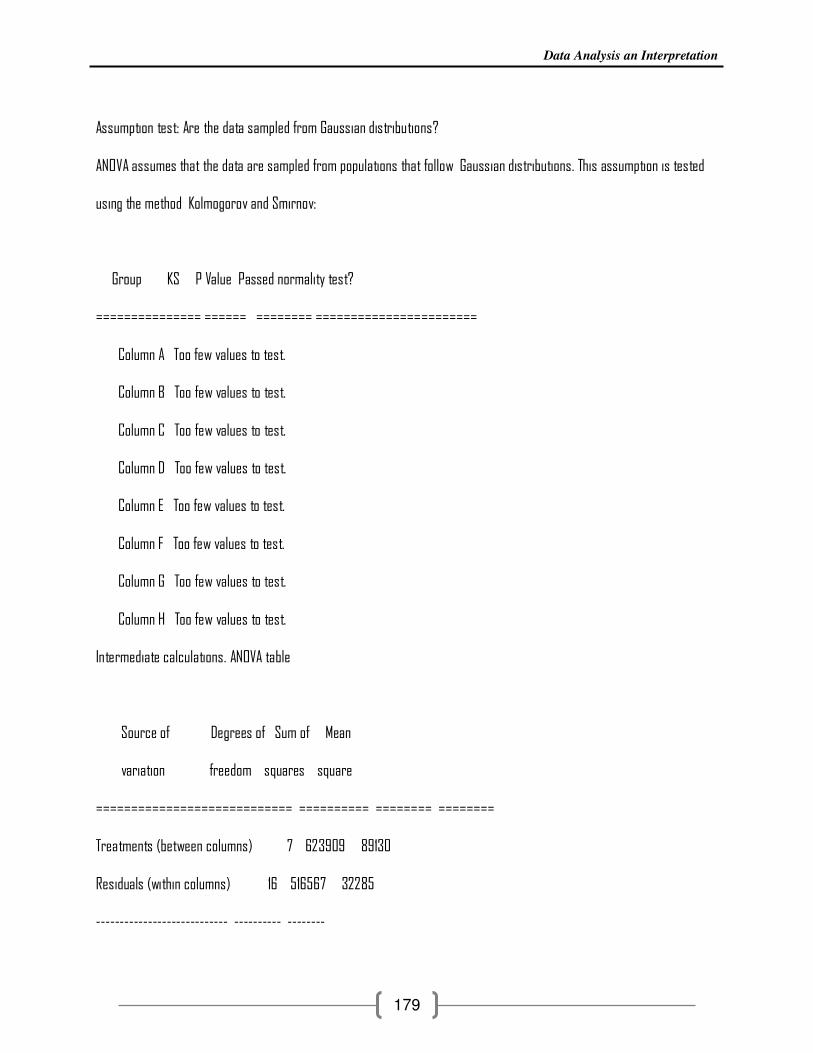
Assumption test: Are the data sampled from Gaussian distributions?
ANOVA assumes that the data are sampled from populations that follow Gaussian distributions. This assumption is tested
using the method Kolmogorov and Smirnov:
Group KS P Value Passed normality test?
=============== ====== ======== =======================
Column A Too few values to test.
Column B Too few values to test.
Column C Too few values to test.
Column D Too few values to test.
Column E Too few values to test.
Column F Too few values to test.
Column G Too few values to test.
Column H Too few values to test.
Intermediate calculations. ANOVA table
Source of Degrees of Sum of Mean
variation freedom squares square
============================ ========== ======== ========
Treatments (between columns) 7 623909 89130
Residuals (within columns) 16 516567 32285
---------------------------- ---------- --------

Data Analysis an Interpretation
180
Total 23 1140476
F = 2.761 =(MStreatment/MSresidual)
Summary of Data
Number Standard
of Standard Error of
Group Points Mean Deviation Mean Median
=============== ====== ======== ========= ======== ========
Column A 3 496.00 418.36 241.54 476.00
Column B 3 173.33 112.10 64.718 208.00
Column C 3 380.00 222.57 128.50 318.00
Column D 3 313.00 108.51 62.650 258.00
Column E 3 82.667 66.463 38.372 118.00
Column F 3 221.33 67.892 39.198 234.00
Column G 3 8.000 7.550 4.359 7.000
Column H 3 41.667 17.214 9.939 36.000
95% Confidence Interval
Group Minimum Maximum From To
=============== ======== ======== ========== ==========
Column A 88.000 924.00 -543.34 1535.3
Column B 48.000 264.00 -105.15 451.82
Column C 195.00 627.00 -172.95 932.95

Data Analysis an Interpretation
181
Column D 243.00 438.00 43.418 582.58
Column E 6.000 124.00 -82.450 247.78
Column F 148.00 282.00 52.666 390.00
Column G 1.000 16.000 -10.756 26.756
Column H 28.000 61.000 -1.100 84.433
* * *
As The P value is 0.0439and is very significant, central hypothesis Ho which states that
the employees in the Public sector have higher level of satisfaction as compared to the Private
sector is accepted and proved.
Table 3.3 Respondents Opinion Related With Career Advancement
Excellent Good Average Poor Q.No Question
Public
Univ
Private
Univ
Public
Univ
Private
Univ
Public
Univ
Private
Univ
Public
Univ
Private
Univ
Q2 How positive are your
interactions with other
members of the
university?
114 109 105 102 63 28 18 61
Q3 How effectively do you
feel your talents are
being used in the
university?
45 118 129 134 77 21 49 27
Data Analysis an Interpretation
182
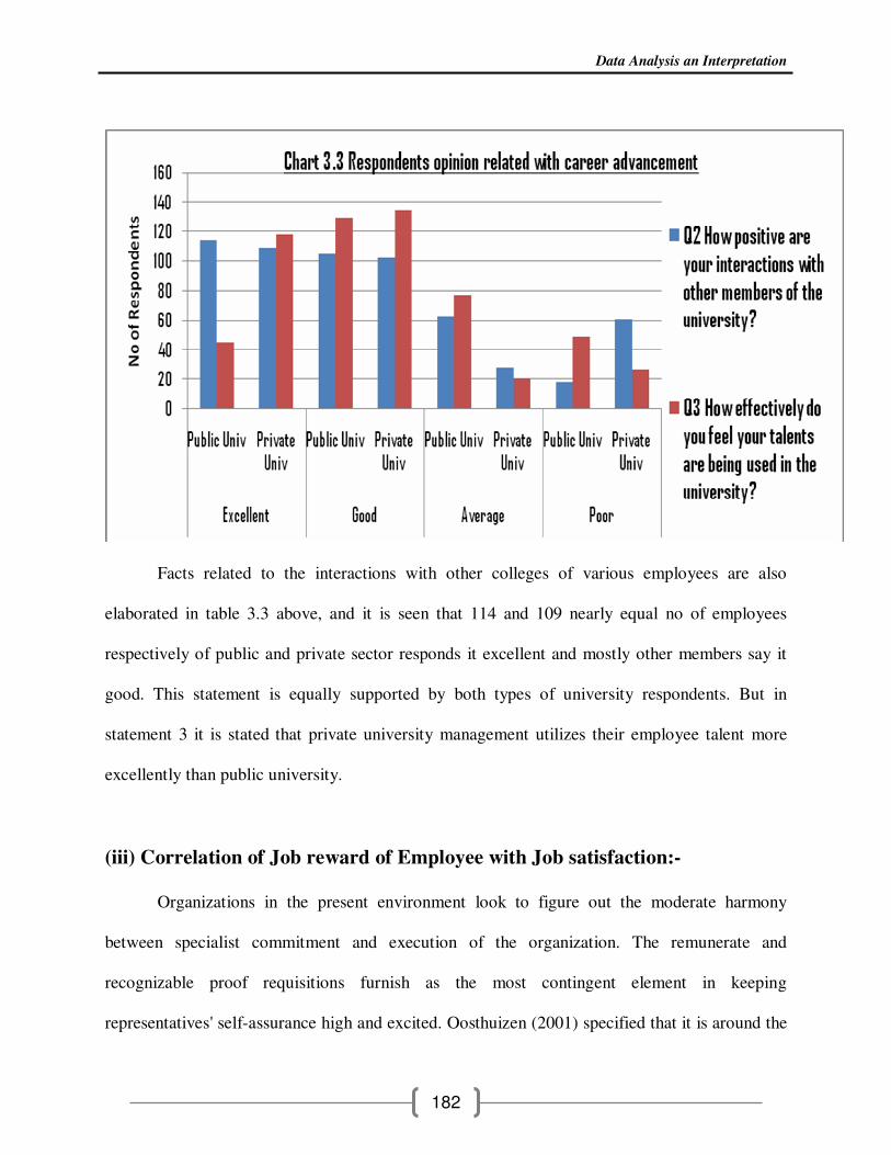
Facts related to the interactions with other colleges of various employees are also
elaborated in table 3.3 above, and it is seen that 114 and 109 nearly equal no of employees
respectively of public and private sector responds it excellent and mostly other members say it
good. This statement is equally supported by both types of university respondents. But in
statement 3 it is stated that private university management utilizes their employee talent more
excellently than public university.
(iii) Correlation of Job reward of Employee with Job satisfaction:-
Organizations in the present environment look to figure out the moderate harmony
between specialist commitment and execution of the organization. The remunerate and
recognizable proof requisitions furnish as the most contingent element in keeping
representatives' self-assurance high and excited. Oosthuizen (2001) specified that it is around the

Data Analysis an Interpretation
183
capacity of directors to energize the laborers effectively and sway their activities to accomplish
more terrific business execution. La Motta (1995) is of the view that execution at occupation is
the consequence of ability and enthusiasm. Capacity created through instruction, gear, preparing,
background, straightforwardness in assignment and two sorts of abilities i.e. mental and physical.
The execution appraisal and profits are the components that ended up being the association
suppliers of the execution evaluation requisitions. As per Wilson (1994), the procedure of
execution administration is one around the key segments of sum repay framework.
Thus to analyze the balance and find out the gaps between Job reward of Employee with
Job satisfaction in the current research design a set of questions are set in section c which are
been elaborated below:-
Data Analysis an Interpretation
184
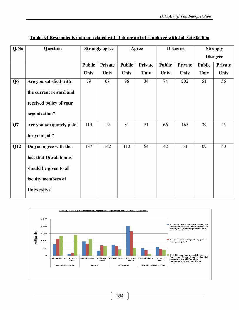
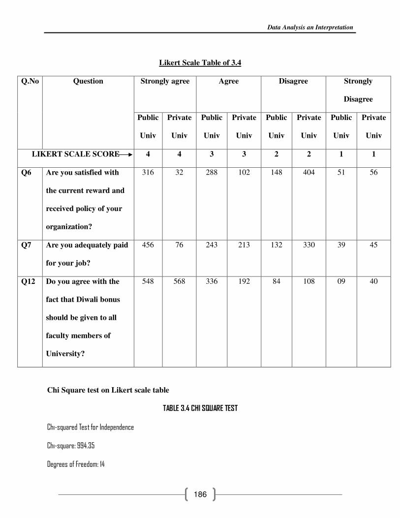
Table 3.4 Respondents opinion related with Job reward of Employee with Job satisfaction
Strongly agree Agree Disagree Strongly
Disagree
Q.No Question
Public
Univ
Private
Univ
Public
Univ
Private
Univ
Public
Univ
Private
Univ
Public
Univ
Private
Univ
Q6 Are you satisfied with
the current reward and
received policy of your
organization?
79 08 96 34 74 202 51 56
Q7 Are you adequately paid
for your job?
114 19 81 71 66 165 39 45
Q12 Do you agree with the
fact that Diwali bonus
should be given to all
faculty members of
University?
137 142 112 64 42 54 09 40

Data Analysis an Interpretation
185
All employees are working for any organization for an financial reward in the form of
salary, bonus etc. If an organization’s employees are well paid in time than on a whole the job
satisfaction level of employees of that organization will always be on higher grounds. Thus in the
current study this section c of the questionnaire deals with respondents opinion towards job
reward policy. It is obtained from the above facts that 202 i.e 75% of private university faculties
are dissatisfied with the reward or salary they are being provided but on contrary 79 of public
university are highly satisfied.
114 out of 300 respondents of public university states that they are adequately paid for
their job , whereas on the other side 165 out of 3000 of private university employees say that
they disagree with the payment norms of university. Diwali bonus is appreciated and admired by
nearly all the employees of public as well as private university. The results obtained from the
above table can be useful for statistical analysis of hypothesis H2: The indicators of Job
satisfaction like salaries, fringe benefits, social security, etc are more favorable in Public
sector.
Statistical analysis:-
To prove the hypothesis by Statistical analytical test after applying Likerts scale
interpretation the frequency was analyzed with Chi Square Test (Goodness of fit Test)
Likert Scale= Rank 4 is good that means is holds more significance as satisfaction parameter
towards job and rank is decreasing its expectancy. Therefore in scoring it can be observed that
the rank is correlated with the score obtained in Likert scale. The mean and max and minimum
limit for each item in Likerts scale is collected.
Data Analysis an Interpretation
186
Likert Scale Table of 3.4
Strongly agree Agree Disagree Strongly
Disagree
Q.No Question
Public
Univ
Private
Univ
Public
Univ
Private
Univ
Public
Univ
Private
Univ
Public
Univ
Private
Univ
LIKERT SCALE SCORE 4 4 3 3 2 2 1 1
Q6 Are you satisfied with
the current reward and
received policy of your
organization?
316 32 288 102 148 404 51 56
Q7 Are you adequately paid
for your job?
456 76 243 213 132 330 39 45
Q12 Do you agree with the
fact that Diwali bonus
should be given to all
faculty members of
University?
548 568 336 192 84 108 09 40
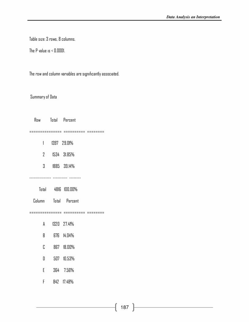
Chi Square test on Likert scale table
TABLE 3.4 CHI SQUARE TEST
Chi-squared Test for Independence
Chi-square: 994.35
Degrees of Freedom: 14
Data Analysis an Interpretation
187
Table size: 3 rows, 8 columns.
The P value is < 0.0001.
The row and column variables are significantly associated.
Summary of Data
Row Total Percent
=============== ========== ========
1 1397 29.01%
2 1534 31.85%
3 1885 39.14%
--------------- ---------- --------
Total 4816 100.00%
Column Total Percent
=============== ========== ========
A 1320 27.41%
B 676 14.04%
C 867 18.00%
D 507 10.53%
E 364 7.56%
F 842 17.48%

Data Analysis an Interpretation
188
G 99 2.06%
H 141 2.93%
--------------- ---------- --------
Total 4816 100.00%
* * *
Interpretation-
The above Goodness of Fit Tests interoperates that the Chi-squared for trend = 994.35 (14 degree
of freedom) The P value is < 0.0001 and very significant .This means that hypothesis H2: The
indicators of Job satisfaction like salaries, fringe benefits, social security, etc are more
favorable in Public sector is accepted and proved.
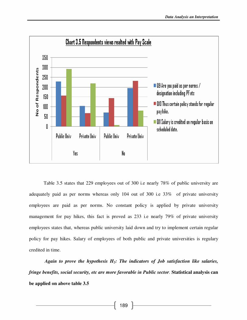
Table 3.5 Respondents opinion related with pay norms
Yes No
Public
Univ
Private
Univ
Public
Univ
Private
Univ
Q9 Are you paid as per norms /
designation including PF etc
229 104 71 196
Q10 Thus certain policy stands for regular
pay hike.
157 67 143 233
Q11 Salary is credited on regular basis on
scheduled date.
294 219 06 81
Data Analysis an Interpretation
189
Table 3.5 states that 229 employees out of 300 i.e nearly 78% of public university are
adequately paid as per norms whereas only 104 out of 300 i.e 33% of private university
employees are paid as per norms. No constant policy is applied by private university
management for pay hikes, this fact is proved as 233 i.e nearly 79% of private university
employees states that, whereas public university laid down and try to implement certain regular
policy for pay hikes. Salary of employees of both public and private universities is regulary
credited in time.
Again to prove the hypothesis H2: The indicators of Job satisfaction like salaries,
fringe benefits, social security, etc are more favorable in Public sector. Statistical analysis can
be applied on above table 3.5
Data Analysis an Interpretation
190
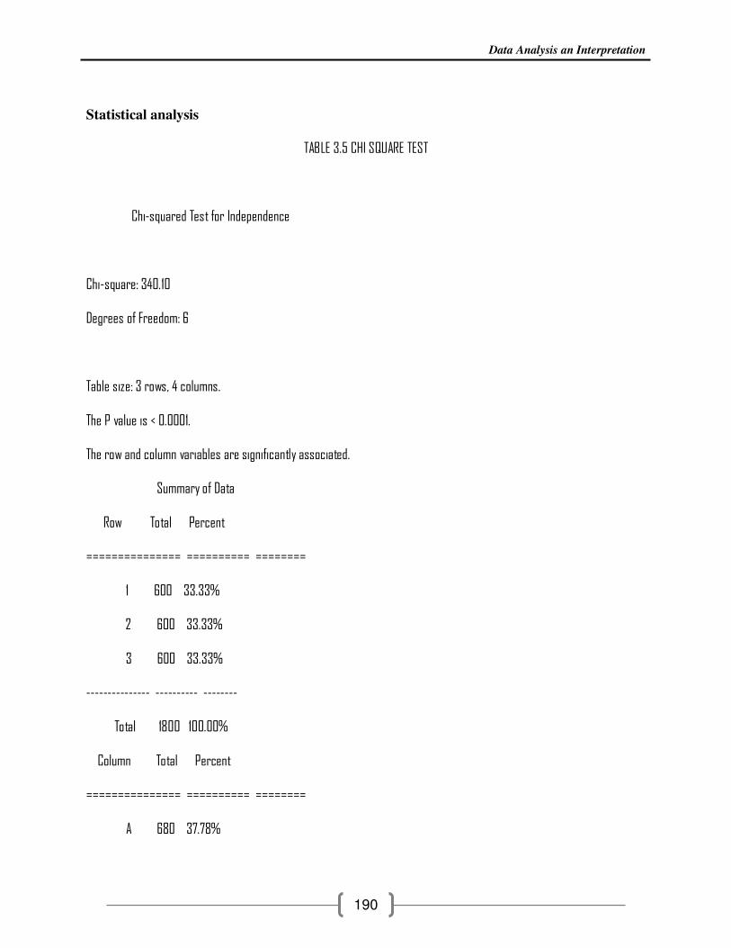
Statistical analysis
TABLE 3.5 CHI SQUARE TEST
Chi-squared Test for Independence
Chi-square: 340.10
Degrees of Freedom: 6
Table size: 3 rows, 4 columns.
The P value is < 0.0001.
The row and column variables are significantly associated.
Summary of Data
Row Total Percent
=============== ========== ========
1 600 33.33%
2 600 33.33%
3 600 33.33%
--------------- ---------- --------
Total 1800 100.00%
Column Total Percent
=============== ========== ========
A 680 37.78%

Data Analysis an Interpretation
191
B 390 21.67%
C 220 12.22%
D 510 28.33%
--------------- ---------- --------
Total 1800 100.00%
* * *
Interpretation
The above Goodness of Fit Tests interoperates that the Chi-squared for trend = 340.10 (6 degree
of freedom) The P value is < 0.0001 and very significant .This means that hypothesis H2: The
indicators of Job satisfaction like salaries, fringe benefits, social security, etc are more
favorable in Public sector is accepted and proved.
(iv) Correlation of Work Life balance of Employee with Job satisfaction:-
Psychologists define life balance as a division of energy between the different aspects of
a person's life, especially family, friends and work. A few driven individuals are happiest when
focused on one element of their lives, but most people need to find a balance. Too much
emphasis on work frequently results in feelings of loneliness and frustration. But not enough
emphasis on work prevents your employees from advancing and you from getting needed work
done. Acknowledging each employee's efforts to strike a balance allows you to be part of the
solution. Job satisfaction typically increases with improved life balance, which in turn increases
employee loyalty, creativity and productivity. Therefore to analyze the role of work life balance
and on job satisfaction section D of the questionnaire is planned in current research and
illuminated below:-

Data Analysis an Interpretation
192
Table 3.6 Respondents opinion related with Work Life balance and job satisfaction
Strongly agree Agree Disagree Strongly Disagree Q.No Question
Public
Univ
Private
Univ
Public
Univ
Private
Univ
Public
Univ
Private
Univ
Public
Univ
Private
Univ
Q13 Is the working
Environment Healthy
and Energetic?
78 51 108 92 62 116 52 41
Q14 Is the job interesting? 119 29 79 68 54 154 48 49
Q16 Are you fairly well-
satisfied with your
present job?
157 103 85 94 53 69 05 34
Q18 Are you satisfied with
your job profile?
128 92 108 114 52 79 12 15

Data Analysis an Interpretation
193
To prove the hypothesis H3: The quality of work-life balance is better in Public sector
employees as compared to Private sector employees , results obtained in above table 3.6 are
statistically studied with the help of Likert’s scale.
Statistical Analysis: To prove the hypothesis by Statistical analytical test after applying
Likerts scale interpretation the frequency was analyzed with one way ANOVA
Likert Scale= Rank 4 is good that means is holds more significance as satisfaction parameter
towards job and rank is decreasing its expectancy. Therefore in scoring it can be observed that
Data Analysis an Interpretation
194
the rank is correlated with the score obtained in Likert scale. The mean and max and minimum
limit for each item in Likerts scale is collected. The Likert Scale Frequency table used for
statistical analysis is as below:-
Likert Scale Table of 3.6
Strongly agree Agree Disagree Strongly Disagree Q.No Question
Public
Univ
Private
Univ
Public
Univ
Private
Univ
Public
Univ
Private
Univ
Public
Univ
Private
Univ
LIKERT SCALE SCORE 4 4 3 3 2 2 1 1
Q13 Is the working
Environment Healthy
and Energetic?
312 204 324 276 124 232 52 41
Q14 Is the job interesting? 476 116 237 204 108 308 48 49
Q16 Are you fairly well-
satisfied with your
present job?
628 412 255 282 106 138 05 34
Q18 Are you satisfied with
your job profile?
512 368 324 342 104 158 12 15
TABLE 3.6 LIKERT SCALE TABLE ANOVA TEST
One-way Analysis of Variance (ANOVA)
The P value is < 0.0001, considered extremely significant.
Variation among column means is significantly greater than expected by chance.
Data Analysis an Interpretation
195
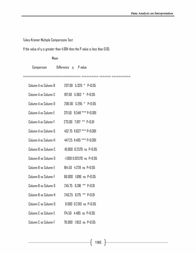
Tukey-Kramer Multiple Comparisons Test
If the value of q is greater than 4.684 then the P value is less than 0.05.
Mean
Comparison Difference q P value
================================== ========== ======= ===========
Column A vs Column B 207.00 5.320 * P<0.05
Column A vs Column C 197.00 5.063 * P<0.05
Column A vs Column D 206.00 5.295 * P<0.05
Column A vs Column E 371.50 9.548 *** P<0.001
Column A vs Column F 273.00 7.017 ** P<0.01
Column A vs Column G 452.75 11.637 *** P<0.001
Column A vs Column H 447.25 11.495 *** P<0.001
Column B vs Column C -10.000 0.2570 ns P>0.05
Column B vs Column D -1.000 0.02570 ns P>0.05
Column B vs Column E 164.50 4.228 ns P>0.05
Column B vs Column F 66.000 1.696 ns P>0.05
Column B vs Column G 245.75 6.316 ** P<0.01
Column B vs Column H 240.25 6.175 ** P<0.01
Column C vs Column D 9.000 0.2313 ns P>0.05
Column C vs Column E 174.50 4.485 ns P>0.05
Column C vs Column F 76.000 1.953 ns P>0.05

Data Analysis an Interpretation
196
Column C vs Column G 255.75 6.573 ** P<0.01
Column C vs Column H 250.25 6.432 ** P<0.01
Column D vs Column E 165.50 4.254 ns P>0.05
Column D vs Column F 67.000 1.722 ns P>0.05
Column D vs Column G 246.75 6.342 ** P<0.01
Column D vs Column H 241.25 6.201 ** P<0.01
Column E vs Column F -98.500 2.532 ns P>0.05
Column E vs Column G 81.250 2.088 ns P>0.05
Column E vs Column H 75.750 1.947 ns P>0.05
Column F vs Column G 179.75 4.620 ns P>0.05
Column F vs Column H 174.25 4.479 ns P>0.05
Column G vs Column H -5.500 0.1414 ns P>0.05
Mean 95% Confidence Interval
Difference Difference From To
================================== ========== ======= =======
Column A - Column B 207.00 24.757 389.24
Column A - Column C 197.00 14.757 379.24
Column A - Column D 206.00 23.757 388.24
Column A - Column E 371.50 189.26 553.74
Column A - Column F 273.00 90.757 455.24
Column A - Column G 452.75 270.51 634.99

Data Analysis an Interpretation
197
Column A - Column H 447.25 265.01 629.49
Column B - Column C -10.000 -192.24 172.24
Column B - Column D -1.000 -183.24 181.24
Column B - Column E 164.50 -17.743 346.74
Column B - Column F 66.000 -116.24 248.24
Column B - Column G 245.75 63.507 427.99
Column B - Column H 240.25 58.007 422.49
Column C - Column D 9.000 -173.24 191.24
Column C - Column E 174.50 -7.743 356.74
Column C - Column F 76.000 -106.24 258.24
Column C - Column G 255.75 73.507 437.99
Column C - Column H 250.25 68.007 432.49
Column D - Column E 165.50 -16.743 347.74
Column D - Column F 67.000 -115.24 249.24
Column D - Column G 246.75 64.507 428.99
Column D - Column H 241.25 59.007 423.49
Column E - Column F -98.500 -280.74 83.743
Column E - Column G 81.250 -100.99 263.49
Column E - Column H 75.750 -106.49 257.99
Column F - Column G 179.75 -2.493 361.99
Column F - Column H 174.25 -7.993 356.49
Column G - Column H -5.500 -187.74 176.74

Data Analysis an Interpretation
198
Assumption test: Are the standard deviations of the groups equal?
ANOVA assumes that the data are sampled from populations with identical
SDs. This assumption is tested using the method of Bartlett.
Bartlett statistic (corrected) = 25.342
The P value is 0.0007.
Bartlett's test suggests that the differences among the SDs is extremely significant.
Since ANOVA assumes populations with equal SDs, you should consider transforming your data (reciprocal or log) or
selecting a nonparametric test.
Assumption test: Are the data sampled from Gaussian distributions?
ANOVA assumes that the data are sampled from populations that follow Gaussian distributions. This assumption is tested
using the method Kolmogorov and Smirnov:
Group KS P Value Passed normality test?
=============== ====== ======== =======================
Column A Too few values to test.
Column B Too few values to test.
Column C Too few values to test.
Column D Too few values to test.
Column E Too few values to test.
Column F Too few values to test.
Column G Too few values to test.

Data Analysis an Interpretation
199
Column H Too few values to test.
Intermediate calculations. ANOVA table
Source of Degrees of Sum of Mean
variation freedom squares square
============================ ========== ======== ========
Treatments (between columns) 7 645666 92238
Residuals (within columns) 24 145325 6055.2
---------------------------- ---------- --------
Total 31 790991
F = 15.233 =(MStreatment/MSresidual)
Summary of Data
Number Standard
of Standard Error of
Group Points Mean Deviation Mean Median
=============== ====== ======== ========= ======== ========
Column A 4 482.00 130.58 65.289 494.00
Column B 4 275.00 138.73 69.366 286.00
Column C 4 285.00 45.629 22.814 289.50
Column D 4 276.00 56.498 28.249 279.00
Column E 4 110.50 9.147 4.573 107.00

Data Analysis an Interpretation
200
Column F 4 209.00 77.399 38.700 195.00
Column G 4 29.250 24.185 12.093 30.000
Column H 4 34.750 14.523 7.261 37.500
95% Confidence Interval
Group Minimum Maximum From To
=============== ======== ======== ========== ==========
Column A 312.00 628.00 274.25 689.75
Column B 116.00 412.00 54.277 495.72
Column C 237.00 324.00 212.40 357.60
Column D 204.00 342.00 186.11 365.89
Column E 104.00 124.00 95.947 125.05
Column F 138.00 308.00 85.858 332.14
Column G 5.000 52.000 -9.228 67.728
Column H 15.000 49.000 11.644 57.856
* * *
As The P value is is 0.0007 and is extremely significant, hypothesis H3 which states that
the quality of work-life balance is better in Public sector employees as compared to Private
sector employees is accepted and proved.

Data Analysis an Interpretation
201
Table 3.7 Respondents opinion related with Work and job satisfaction
Strongly agree Agree Disagree Strongly Disagree Q.No Question
Public
Univ
Private
Univ
Public
Univ
Private
Univ
Public
Univ
Private
Univ
Public
Univ
Private
Univ
Q15 Are you enthusiastic
about your work
119 132 101 113 21 39 59 16
Q17 Do you think each
day of work seems
like it will never end?
54 132 124 106 51 23 71 39
Q19 Do you enjoy at your
work?
147 113 95 84 43 59 15 44

Data Analysis an Interpretation
202
Hypothesis H4: Private sector employees have more exposure of working in various sectors
such as Administrative etc. is analysed with the help of results obtained in table 3.7 above.
Statistical analysis: To prove the hypothesis by Statistical analytical test after applying
Likerts scale interpretation the frequency was analyzed with Chi Square Test (Goodness of fit
Test)
Likert Scale= Rank 4 is good that means is holds more significance as satisfaction parameter
towards job and rank is decreasing its expectancy. Therefore in scoring it can be observed that
the rank is correlated with the score obtained in Likert scale. The mean and max and minimum
limit for each item in Likerts scale is collected.
Likert Scale Table of 3.7
Strongly agree Agree Disagree Strongly Disagree Q.No Question
Public
Univ
Private
Univ
Public
Univ
Private
Univ
Public
Univ
Private
Univ
Public
Univ
Private
Univ
LIKERT SCALE SCORE 4 4 3 3 2 2 1 1
Q15 Are you enthusiastic
about your work
476 528 303 339 42 78 59 16
Q17 Do you think each
day of work seems
like it will never end?
216 528 372 318 102 46 71 39
Q19 Do you enjoy at your
work?
588 452 285 252 86 118 15 44

Data Analysis an Interpretation
203
TABLE 3.7 CHI SQUARE TEST ON LIKERT SCALE TABLE
Chi-squared Test for Independence
Chi-square: 308.04
Degrees of Freedom: 14
Table size: 3 rows, 8 columns.
The P value is < 0.0001.
The row and column variables are significantly associated.
Summary of Data
Row Total Percent
=============== ========== ========
1 1841 34.26%
2 1692 31.49%
3 1840 34.25%
--------------- ---------- --------
Total 5373 100.00%
Column Total Percent
=============== ========== ========
A 1280 23.82%
B 1508 28.07%
C 960 17.87%
D 909 16.92%
Data Analysis an Interpretation
204
E 230 4.28%
F 242 4.50%
G 145 2.70%
H 99 1.84%
--------------- ---------- --------
Total 5373 100.00%
Interpretation-
The above Goodness of Fit Tests interoperates that the Chi-squared for trend = 308 (14
degree of freedom) The P value is < 0.0001 and very significant .This means that hypothesis H4:
Private sector employees have more exposure of working in various sectors such as
Administrative is accepted and proved.
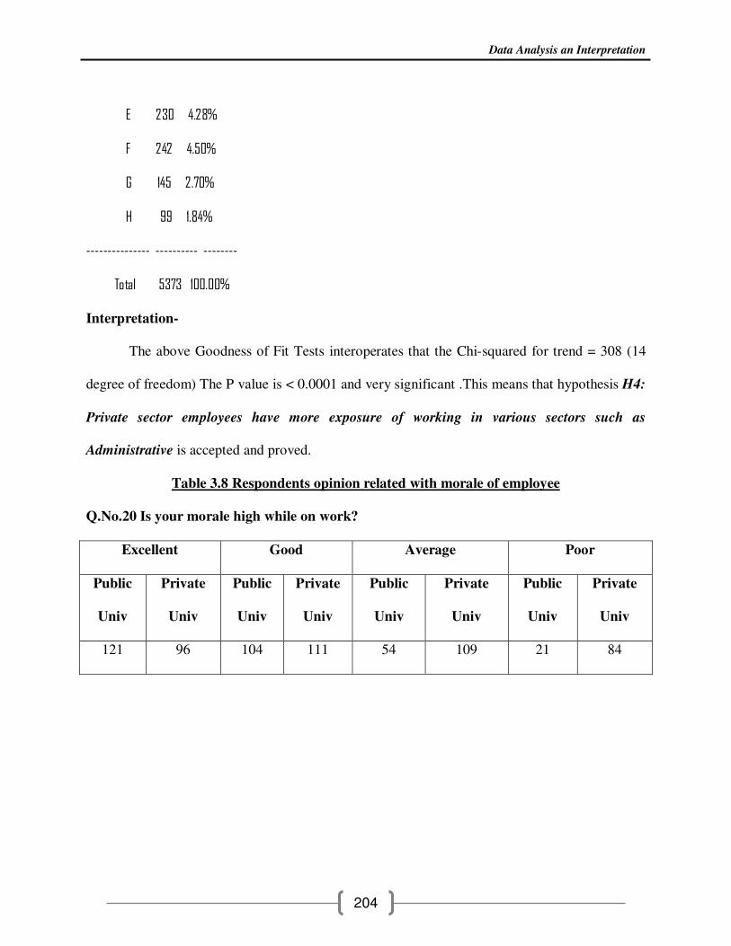
Table 3.8 Respondents opinion related with morale of employee
Q.No.20 Is your morale high while on work?
Excellent Good Average Poor
Public
Univ
Private
Univ
Public
Univ
Private
Univ
Public
Univ
Private
Univ
Public
Univ
Private
Univ
121 96 104 111 54 109 21 84

Data Analysis an Interpretation
205
40% of public university employee’s morale is excellent while they are on work and 35 % of
same segment of university have good morale to work, but on the other hand only 24 % and 28%
of private university employee’s have high and good morale respectively. But the percentage of
poor morale is 21% in private university employee as compared to only 7% in public university
faculties.
(v) Correlation of Administration / Management of University with Employee
Job satisfaction:-
The connection an worker has with his or her manager is a main factor to the worker's
association to the company, and it has been suggested that many worker actions are mostly a
Data Analysis an Interpretation
206
operate of the way they are handled by their managers. One of the elements of a good connection
is efficient interaction. When there are start collections of interaction (e.g., motivating an open-
door policy), managers can react more successfully to the needs and problems of their workers.
Effective interaction from mature control can offer the employees with route. In addition,
management’s identification of employees’ efficiency through compliment (private or public),
prizes and rewards is a cost-effective way of improving worker spirits, efficiency and
competition. As companies appear from the economic downturn, it is essential for the mature
control team to connect successfully about the company's business objectives, guidelines and
perspective. This will help definitely interact with workers, offer workers with route and promote
believe in and regard. Frequently, workers are involved about the effects of providing forth
recommendations and issues to control. Employees need to be motivated to do so without fear;
otherwise, creativeness and advancement may be stifled. Organizations use different methods to
motivate reviews and interaction between workers and mature management— for example,
worker reviews, focus categories, city area conferences and recommendation containers.
Employees in middle-management roles and nonexempt non control workers recognized this part
to be more essential than did professional non control workers.
Therefore in current research design section E is designed to evaluate the Job satisfaction
relation with Administration / Management, which is been analyzed below:--
Data Analysis an Interpretation
207
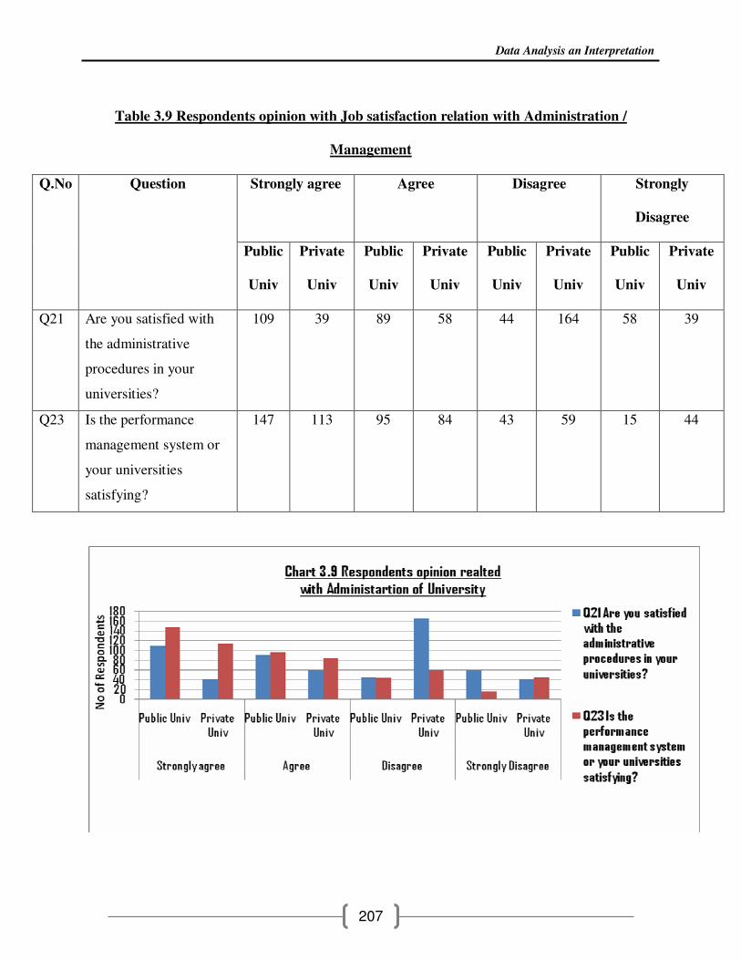
Table 3.9 Respondents opinion with Job satisfaction relation with Administration /
Management
Strongly agree Agree Disagree Strongly
Disagree
Q.No Question
Public
Univ
Private
Univ
Public
Univ
Private
Univ
Public
Univ
Private
Univ
Public
Univ
Private
Univ
Q21 Are you satisfied with
the administrative
procedures in your
universities?
109 39 89 58 44 164 58 39
Q23 Is the performance
management system or
your universities
satisfying?
147 113 95 84 43 59 15 44

Data Analysis an Interpretation
208
Central hypothesis of the research H0The employees in the Public sector have higher
level of satisfaction as compared to the Private sector can be analyzed with the help of above
results obtained in table3.9
Statistical analysis:- To prove the hypothesis by Statistical analytical test after applying
Likerts scale interpretation the frequency was analyzed with Chi Square Test (Goodness of fit
Test)
Likert Scale= Rank 4 is good that means is holds more significance as satisfaction parameter
towards job and rank is decreasing its expectancy. Therefore in scoring it can be observed that
the rank is correlated with the score obtained in Likert scale. The mean and max and minimum
limit for each item in Likerts scale is collected.
Data Analysis an Interpretation
209
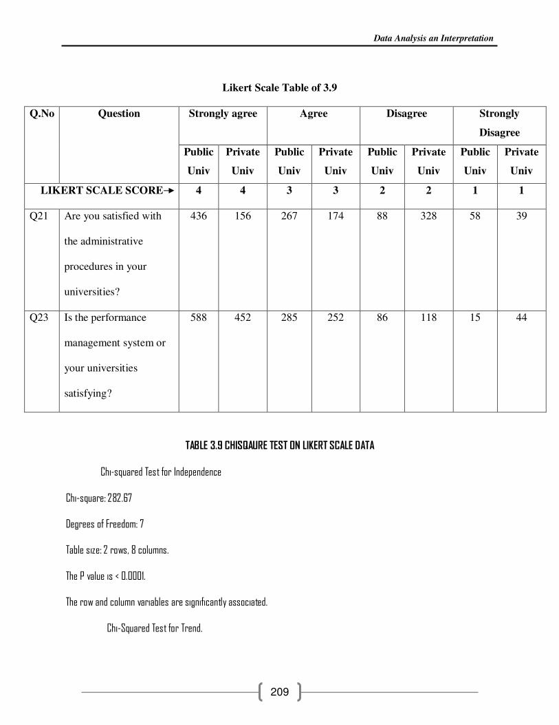
Likert Scale Table of 3.9
Strongly agree Agree Disagree Strongly
Disagree
Q.No Question
Public
Univ
Private
Univ
Public
Univ
Private
Univ
Public
Univ
Private
Univ
Public
Univ
Private
Univ
LIKERT SCALE SCORE 4 4 3 3 2 2 1 1
Q21 Are you satisfied with
the administrative
procedures in your
universities?
436 156 267 174 88 328 58 39
Q23 Is the performance
management system or
your universities
satisfying?
588 452 285 252 86 118 15 44
TABLE 3.9 CHISQAURE TEST ON LIKERT SCALE DATA
Chi-squared Test for Independence
Chi-square: 282.67
Degrees of Freedom: 7
Table size: 2 rows, 8 columns.
The P value is < 0.0001.
The row and column variables are significantly associated.
Chi-Squared Test for Trend.
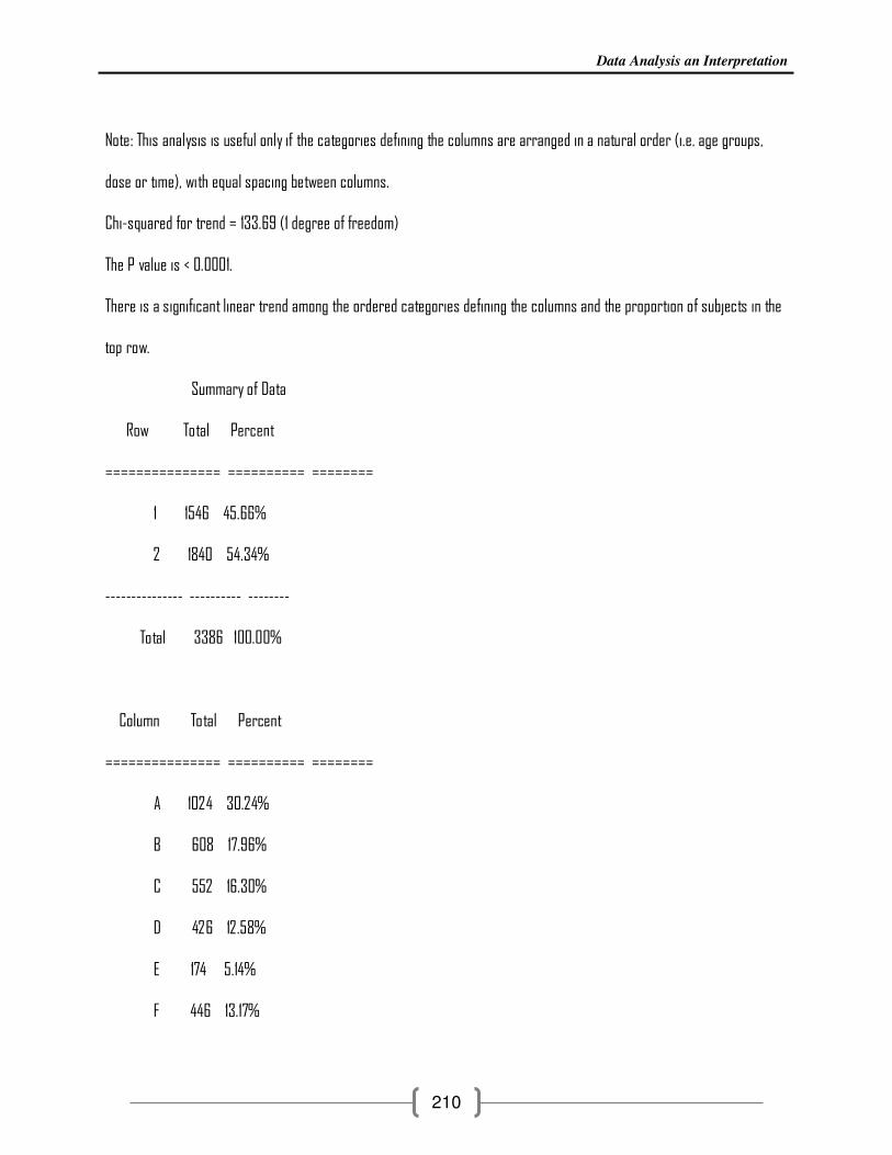
Data Analysis an Interpretation
210
Note: This analysis is useful only if the categories defining the columns are arranged in a natural order (i.e. age groups,
dose or time), with equal spacing between columns.
Chi-squared for trend = 133.69 (1 degree of freedom)
The P value is < 0.0001.
There is a significant linear trend among the ordered categories defining the columns and the proportion of subjects in the
top row.
Summary of Data
Row Total Percent
=============== ========== ========
1 1546 45.66%
2 1840 54.34%
--------------- ---------- --------
Total 3386 100.00%
Column Total Percent
=============== ========== ========
A 1024 30.24%
B 608 17.96%
C 552 16.30%
D 426 12.58%
E 174 5.14%
F 446 13.17%
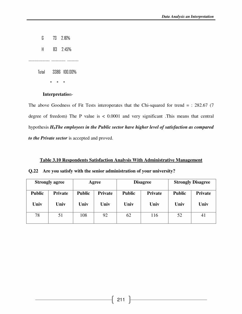
Data Analysis an Interpretation
211
G 73 2.16%
H 83 2.45%
--------------- ---------- --------
Total 3386 100.00%
* * *
Interpretation-
The above Goodness of Fit Tests interoperates that the Chi-squared for trend = : 282.67 (7
degree of freedom) The P value is < 0.0001 and very significant .This means that central
hypothesis H0The employees in the Public sector have higher level of satisfaction as compared
to the Private sector is accepted and proved.
Table 3.10 Respondents Satisfaction Analysis With Administrative Management
Q.22 Are you satisfy with the senior administration of your university?
Strongly agree Agree Disagree Strongly Disagree
Public
Univ
Private
Univ
Public
Univ
Private
Univ
Public
Univ
Private
Univ
Public
Univ
Private
Univ
78 51 108 92 62 116 52 41
Data Analysis an Interpretation
212
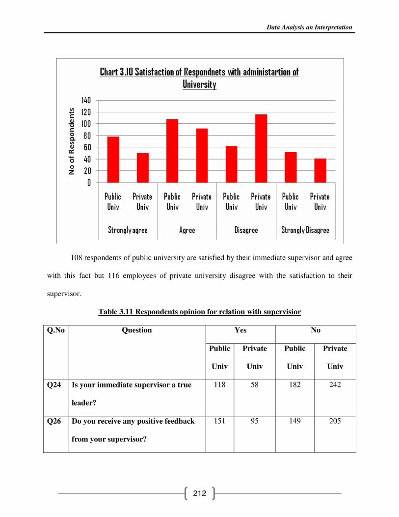
108 respondents of public university are satisfied by their immediate supervisor and agree
with this fact but 116 employees of private university disagree with the satisfaction to their
supervisor.
Table 3.11 Respondents opinion for relation with supervisior
Yes No Q.No Question
Public
Univ
Private
Univ
Public
Univ
Private
Univ
Q24 Is your immediate supervisor a true
leader?
118 58 182 242
Q26 Do you receive any positive feedback
from your supervisor?
151 95 149 205

Data Analysis an Interpretation
213
Relationship of with supervisor can be helpful for making job stable and for the current
study this can be analysed with the help of results obtained in above table 3.11. Thus to prove the
hypothesis, H5: Public sector jobs offer more stability.
Statistical Analysis:
To analyze the above hypothesis two tailed T test is applied on data obtained and
results are as follow:-
TABLE 3.11 Two tailed t test
Unpaired t test
Do the means of Column A and Column B differ significantly?
P value
The two-tailed P value is > 0.9999, considered not significant.
t = 0.000 with 6 degrees of freedom.
95% confidence interval
Mean difference = 0.000 (Mean of Column B minus mean of Column A)
The 95% confidence interval of the difference: -111.75 to 111.75
Assumption test: Are the standard deviations equal?
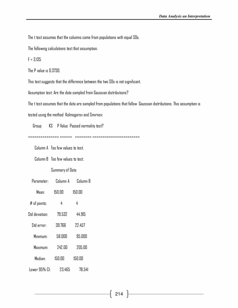
Data Analysis an Interpretation
214
The t test assumes that the columns come from populations with equal SDs.
The following calculations test that assumption.
F = 3.135
The P value is 0.3730.
This test suggests that the difference between the two SDs is not significant.
Assumption test: Are the data sampled from Gaussian distributions?
The t test assumes that the data are sampled from populations that follow Gaussian distributions. This assumption is
tested using the method Kolmogorov and Smirnov:
Group KS P Value Passed normality test?
=============== ====== ======== =======================
Column A Too few values to test.
Column B Too few values to test.
Summary of Data
Parameter: Column A Column B
Mean: 150.00 150.00
# of points: 4 4
Std deviation: 79.532 44.915
Std error: 39.766 22.457
Minimum: 58.000 95.000
Maximum: 242.00 205.00
Median: 150.00 150.00
Lower 95% CI: 23.465 78.541

Data Analysis an Interpretation
215
Upper 95% CI: 276.54 221.46
* * *
Interpretation –
As the two tailed P value is > 0.9999, considered not significant therefore hypothesis H5:
Public sector jobs offer more stability is rejected.
Table 3.12 Opinion for immediate supervisor
Q.25 Are the relation between you and your immediate supervisor is healthy?
Excellent Good Average Poor
Public
Univ
Private
Univ
Public
Univ
Private
Univ
Public
Univ
Private
Univ
Public
Univ
Private
Univ
157 103 85 94 53 69 05 34
Data Analysis an Interpretation
216
52 % of public university employees have excellent relation with their supervisor and
only 35% of private university employees maintain the same. But on contrary the % of poor
relation is 11% for private university employees while only 2% for public university employees.
(vi) Correlation of Infrastructure and Technology of University with
Employee Job satisfaction:-
The workplaces in which workers perform and carry out most of their activities can effect
on their efficiency. The classifieds of perform generated by workers are affected by the
workplaces (Keeling and Kallaus, 1996). While Quible, (1996) points out those poor ecological
conditions can cause ineffective employee efficiency as well as reduce their job fulfillment,
which in turn will effect on the financial well-being of the organization. Most people spend 50%
of their lives within inside surroundings, which greatly influence their mental position, actions,
capabilities and performance (Sundstrom, 1994). Better results and increased efficiency is
believed to be the result of better office atmosphere. Better actual atmosphere of office will
increases the workers and finally improve their efficiency. Various literary works correspond
with the study of multiple workplaces and workplaces shows that the factors such as
discontentment, crazy office structures and the actual atmosphere, loss of employees’ efficiency
(Carnevale, 1992; Clements- Croome, 1997).
Office atmosphere can be separated into two components; actual and behavior. The actual
atmosphere correspond with the office occupiers’ ability to physically link with their workplaces.
The behavior atmosphere is related to how well the office occupiers link with each other, and the
effect the workplaces can have on the behavior of the individual.

Data Analysis an Interpretation
217
The actual atmosphere with the efficiency of its tenant drops into two primary groups
office structure and office comfort, and the behavior atmosphere symbolizes the two primary
elements namely connections and distraction(Amir and Sahibzada, 2010).Employees in different
companies have various office designs.
Every office has unique furniture and spatial arrangements, lighting and heating
arrangements and different levels of noise. This study also analyzes the impact of the
Infrastructure and Technology on employees’ job satisfaction through section F discussed
ahead:-
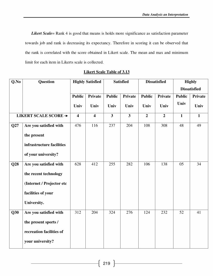
Table 3.13 Respondents opinion related with Infrastructure and Technology
Highly Satisfied Satisfied Dissatisfied Highly
Dissatisfied
Q.No Question
Public
Univ
Private
Univ
Public
Univ
Private
Univ
Public
Univ
Private
Univ
Public
Univ
Private
Univ
Q27 Are you satisfied with
the present
infrastructure facilities
of your university?
119 29 79 68 54 154 48 49
Q28 Are you satisfied with
the recent technology
(Internet / Projector etc
facilities of your
University.
157 103 85 94 53 69 05 34

Data Analysis an Interpretation
218
Q30 Are you satisfied with
the present sports /
recreation facilities of
your university?
78 51 108 92 62 116 52 41
Hypothesis H7: Private sector employees gave better chances and facilities for higher
education in the same university of the current research study can be analyzed by the facts
obtained form table 3.13 above.
Statistical analysis:-
To prove the hypothesis by Statistical analytical test after applying Likerts scale
interpretation the frequency was analyzed with Chi Square Test (Goodness of fit Test)
Data Analysis an Interpretation
219
Likert Scale= Rank 4 is good that means is holds more significance as satisfaction parameter
towards job and rank is decreasing its expectancy. Therefore in scoring it can be observed that
the rank is correlated with the score obtained in Likert scale. The mean and max and minimum
limit for each item in Likerts scale is collected.
Likert Scale Table of 3.13
Highly Satisfied Satisfied Dissatisfied Highly
Dissatisfied
Q.No Question
Public
Univ
Private
Univ
Public
Univ
Private
Univ
Public
Univ
Private
Univ
Public
Univ
Private
Univ
LIKERT SCALE SCORE 4 4 3 3 2 2 1 1
Q27 Are you satisfied with
the present
infrastructure facilities
of your university?
476 116 237 204 108 308 48 49
Q28 Are you satisfied with
the recent technology
(Internet / Projector etc
facilities of your
University.
628 412 255 282 106 138 05 34
Q30 Are you satisfied with
the present sports /
recreation facilities of
your university?
312 204 324 276 124 232 52 41

Data Analysis an Interpretation
220
TABLE 3.13 LIKERT SCALE TABLE CHI SQUARE ANALYSIS
Chi-squared Test for Independence
Chi-square: 385.30
Degrees of Freedom: 14
Table size: 3 rows, 8 columns.
The P value is < 0.0001.
The row and column variables are significantly associated.
Summary of Data
Row Total Percent
=============== ========== ========
1 1546 31.10%
2 1860 37.42%
3 1565 31.48%
--------------- ---------- --------
Total 4971 100.00%
Column Total Percent
=============== ========== ========
A 1416 28.49%
B 732 14.73%
C 816 16.42%

Data Analysis an Interpretation
221
D 762 15.33%
E 338 6.80%
F 678 13.64%
G 105 2.11%
H 124 2.49%
--------------- ---------- --------
Total 4971 100.00%
* * *
Interpretation-
The above Goodness of Fit Tests interoperates that the Chi-squared for trend = 385.30
(14 degree of freedom) The P value is < 0.0001 and very significant .This means that hypothesis
H2: H7: Private sector employees gave better chances and facilities for higher education in the
same university is accepted and proved.
Table 3.14 Respondents opinion for laptop
Q. 29 Thus your University had provided laptop to you.
Type of University Yes No
Public University 102 198
Private University 194 106
Data Analysis an Interpretation
222
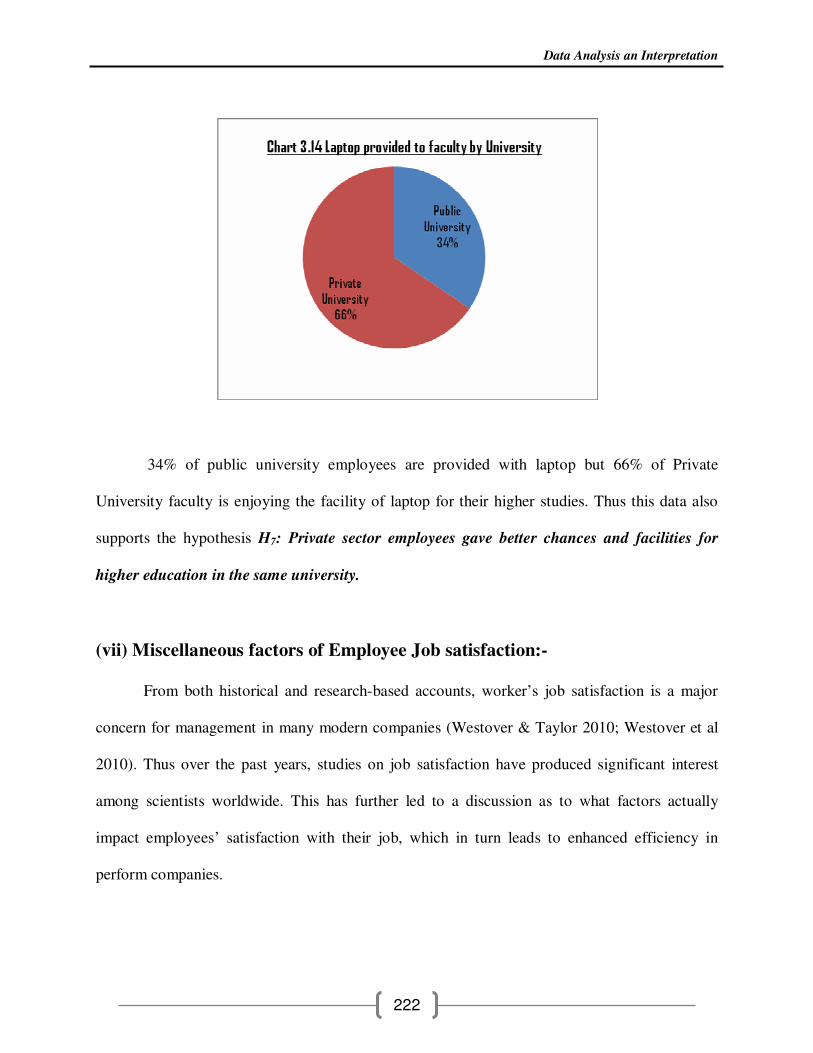
34% of public university employees are provided with laptop but 66% of Private
University faculty is enjoying the facility of laptop for their higher studies. Thus this data also
supports the hypothesis H7: Private sector employees gave better chances and facilities for
higher education in the same university.
(vii) Miscellaneous factors of Employee Job satisfaction:-
From both historical and research-based accounts, worker’s job satisfaction is a major
concern for management in many modern companies (Westover & Taylor 2010; Westover et al
2010). Thus over the past years, studies on job satisfaction have produced significant interest
among scientists worldwide. This has further led to a discussion as to what factors actually
impact employees’ satisfaction with their job, which in turn leads to enhanced efficiency in
perform companies.

Data Analysis an Interpretation
223
While many claim that each business whether small, method or big has its own unique
way of encouraging its workers, job satisfaction of workers can be commonly arranged into five
unique design categories: need satisfaction, inconsistencies, value achievement, value, and
dispositional/genetic elements designs (Kinicki & Kreitner 2007). These are described as: need
satisfaction is in accordance with the satisfaction identified by the level to which a job, with its
specified features and responsibilities, allows an personal employee to meet his/her personal
needs. Second, the difference design describes that satisfaction is a result of met, or sometimes
unmet, objectives. Third, the value achievement designs are in accordance with the fact that
satisfaction comes from the understanding that someone’s job satisfies your perform principles.
4th, the value designs claim that satisfaction is in accordance with the understanding of how
fairly an personal is handled at perform. This is mostly depending on how someone’s own
perform results, comparative to his/her information and initiatives, compare to the input/output
of others in the place of perform, and lastly; the dispositional/genetic elements designs suggest
that personal employee variations are just as important for identifying job satisfaction and
success as office related factors (Kinicki & Kreitner, 2007).
Therefore many miscellaneous factors contributing for job satisfaction of employees in
public and private sector are analyzed below in section G.

Data Analysis an Interpretation
224
Table 3.15 Faculty social benefits from Job
Q.31 Are you socially benefited by your work?
Strongly agree Agree Disagree Strongly Disagree
Public
Univ
Private
Univ
Public
Univ
Private
Univ
Public
Univ
Private
Univ
Public
Univ
Private
Univ
231 52 65 146 03 74 01 28

Data Analysis an Interpretation
225
231 out of 300 respondents of Public Sector University are strongly agree with the fact
that they are socially benefited by their job and 146 out of 300 i.e nearly 50% are agree with the
same. Negligible no of faculty of public and private university say that they are not socially
benefited with the job.
Table 3.16 Respondents opinion for miscellaneous factors and Job satisfaction
Yes No Q.No Question
Public
Univ
Private
Univ
Public
Univ
Private
Univ
Q32 Do you compare your job with your hobby? 114 106 186 194
Q33 Do you find the Job monotonous? 121 169 179 131
Q34 Do you often bored with your job? 142 178 158 122
Q35 Are the resources easily available required
for your job?
214 131 86 169
Q36 Do you get opportunities to increase your
knowledge through training /seminars etc.
202 159 98 141
Q37 Do you recommend your workplace to
others to work?
103 94 197 206
Data Analysis an Interpretation
226
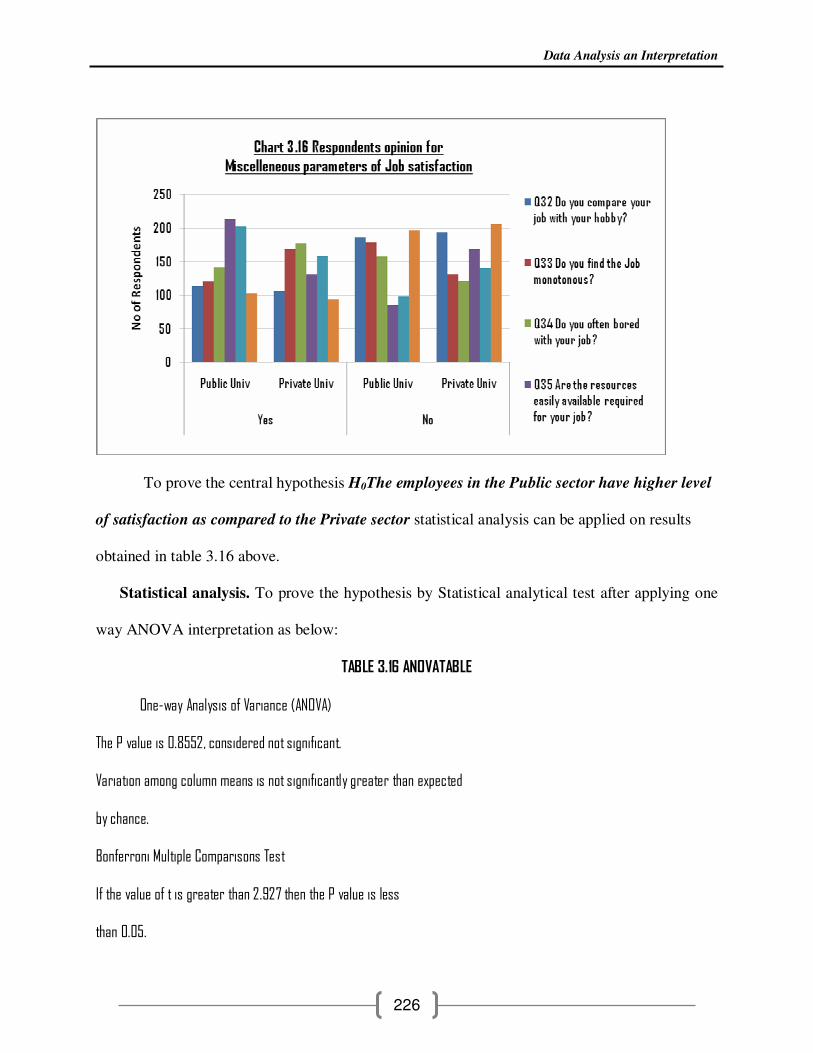
To prove the central hypothesis H0The employees in the Public sector have higher level
of satisfaction as compared to the Private sector statistical analysis can be applied on results
obtained in table 3.16 above.
Statistical analysis. To prove the hypothesis by Statistical analytical test after applying one
way ANOVA interpretation as below:
TABLE 3.16 ANOVATABLE
One-way Analysis of Variance (ANOVA)
The P value is 0.8552, considered not significant.
Variation among column means is not significantly greater than expected
by chance.
Bonferroni Multiple Comparisons Test
If the value of t is greater than 2.927 then the P value is less
than 0.05.

Data Analysis an Interpretation
227
Mean
Comparison Difference t P value
================================== ========== ======= ===========
Column A vs Column B 9.833 0.4106 ns P>0.05
Column A vs Column C -1.333 0.05568 ns P>0.05
Column A vs Column D -11.167 0.4663 ns P>0.05
Column B vs Column C -11.167 0.4663 ns P>0.05
Column B vs Column D -21.000 0.8769 ns P>0.05
Column C vs Column D -9.833 0.4106 ns P>0.05
Mean 95% Confidence Interval
Difference Difference From To
================================== ========== ======= =======
Column A - Column B 9.833 -60.264 79.931
Column A - Column C -1.333 -71.431 68.764
Column A - Column D -11.167 -81.264 58.931
Column B - Column C -11.167 -81.264 58.931
Column B - Column D -21.000 -91.097 49.097
Column C - Column D -9.833 -79.931 60.264
Assumption test: Are the standard deviations of the groups equal?
ANOVA assumes that the data are sampled from populations with identical SDs. This assumption is tested using the method
of Bartlett.

Data Analysis an Interpretation
228
Bartlett statistic (corrected) = 0.8878
The P value is 0.8284.
Bartlett's test suggests that the differences among the SDs is not significant.
Assumption test: Are the data sampled from Gaussian distributions?
ANOVA assumes that the data are sampled from populations that follow Gaussian distributions. This assumption is tested
using the method Kolmogorov and Smirnov:
Group KS P Value Passed normality test?
=============== ====== ======== =======================
Column A 0.2282 >0.10 Yes
Column B 0.2133 >0.10 Yes
Column C 0.2282 >0.10 Yes
Column D 0.2133 >0.10 Yes
Intermediate calculations. ANOVA table
Source of Degrees of Sum of Mean
variation freedom squares square
============================ ========== ======== ========
Treatments (between columns) 3 1328.3 442.78
Residuals (within columns) 20 34410 1720.5
---------------------------- ---------- --------
Total 23 35738
F = 0.2574 =(MStreatment/MSresidual)
Summary of Data
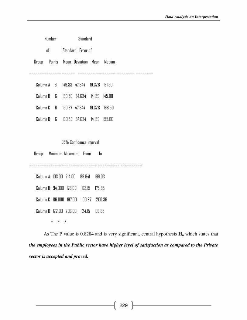
Data Analysis an Interpretation
229
Number Standard
of Standard Error of
Group Points Mean Deviation Mean Median
=============== ====== ======== ========= ======== ========
Column A 6 149.33 47.344 19.328 131.50
Column B 6 139.50 34.634 14.139 145.00
Column C 6 150.67 47.344 19.328 168.50
Column D 6 160.50 34.634 14.139 155.00
95% Confidence Interval
Group Minimum Maximum From To
=============== ======== ======== ========== ==========
Column A 103.00 214.00 99.641 199.03
Column B 94.000 178.00 103.15 175.85
Column C 86.000 197.00 100.97 200.36
Column D 122.00 206.00 124.15 196.85
* * *
As The P value is 0.8284 and is very significant, central hypothesis Ho which states that
the employees in the Public sector have higher level of satisfaction as compared to the Private
sector is accepted and proved.

Data Analysis an Interpretation
230
(viii) RELIABILITY ANALYSIS OF PUBLIC AND PRIVATE SECTOR UNIVERSITY
RESPONDENTS
CRONBACH’S ALPHA PUBLIC SECTOR UNIVERSITY RESPONDENTS
Reliability Statistics----
Cronbach's Alpha N of Items
.723 56
CRONBACH’S ALPHA PRIVATE SECTOR UNIVERSITY RESPONDENTS
Reliability Statistics----
Cronbach's Alpha N of Items
.894 72
The above reliability study indicates that the public and private sector university respondent’s
responses are reliable up to significant level and free from biases.
Data Analysis an Interpretation
231
REFERENCES
1. Agarwal, B.L. (2009) Basic Statistics, pp. 809, New Age International Publisher, New
Delhi.
2. Ahuja Ram (2001) Research Methods. pp. 454, Rawat Publications, Jaipur.
3. Ahuja, Ram (2006): Social Problemin India , pp. 369 Rawat Publication, Jaipur
4. Allen Mike (2008) Quantitative Research in Communication, pp. 245, Sage Publications,
California.:
5. Ambastha, C.K.( 2001) Communication Patterns in Innovation Development, Extension
and Client System, B. R. Publishing Corporation, Delhi.
6. Appadurai, Arjun.(1997), Modernity At Large, p.229,Cultural Dimensions of
Globalization. New Delhi.
7. Arthur, J. (1994). Effects of human resources systems on manufacturing performance and
turnover. Academy of Management Journal , 37, pp. 670-687.
8. Barak, B. and L.G. Schiffman, (1981), Cognitive Age: A Nonchronological Age
Variable," in Advances in Consumer Research, Jrnll of mktg prectice,5, pp. 248-261.
Abugre, J.B. (2011). Perceived Satisfaction in Sustained Outcomes of Employee
Communication in Ghanaian Organizations, Journal of Management Policy and Practice
vol. 12(7), 37-49.
9. Borzaga, C., & Tortia, E. (2006). Worker Motivations,Job Satisfaction, and Loyalty in
Public and Non - Profit Social Services. Nonprofit and Voluntary Sector Quaterly , 35
(2), pp. 225-248.
10. Creswell and W. John (2002) Research Design, pp. 272,Sage Publications (CA)

Data Analysis an Interpretation
232
11. Driscoll, M., & Randall, D. (1999). Perceived Organizational Support, Satisfaction with
Rewards and Employee Job Involvement and Organizational Commitment. International
Association of Applied Psychology , 48 (2), pp. 197-209.
12. Essa, E. L. (1987) The effects of a computer on preschool activities, Early Childhood
Research Quarterly, 2 (4), pp. 377-382.
13. Freud, Sigmund (1962). A General Introduction to Psychoanalysis. pp. 480,
Washington.Square Press. Gianforte, New York.
14. Gruneberg, M. (1976). Job Satisfaction - A Reader. London: Macmillan Press.
15. Herzberg, F. M. (1959). The Motivation to Work (2nd ed.). New York: Wiley.
16. Heskett, J., Sasser, W., & Schesinger, L. (1997). The service profit chain: How leading
companies link profit and growth to loyalty,satisfaction, and value. New York : Free
Press .
17. Heskett, J., Sasser, W., & Schlesinger, L. (1997). The Service Profit Chain: How leading
Companies Link Profit and growth to loyalty, satisfcation and value. New York: Free
Press.
18. Hong Lu, While, E., & Barriball, L. (2005). Job Satisfaction among nurses: a review of
literature. International Journal of Nursing Studies , 42, pp. 211-227.
19. Hostage, G. (1975). Quality control in a service business . Harvard Business Review , pp.
98-106.
20. Kalantzis M. and A. Pandian (2001) Literacy Matters, Issues for New Times, pp.193.
Common Ground. Malaysia.
21. Kallerberg, A. (1977). Work values and job rewards: A theory of job satisfaction.
American Sociological Review , 42 (1), pp. 124-143.

Data Analysis an Interpretation
233
22. Kinicki, A. and Kreitner, R. (2007), Organizational Behavior, McGraw-Hill, New York,
NY.
23. Kinicki, A. J., McKee-Ryan, F. J., Schriesheim, C. A., & Carson, K. P. (2002). Assessing
the construct validity of the Job Descriptive Index: A review and meta-analysis. Journal
of Applied Psychology, 87(1), pp. 14–32.
24. Kothari C.R.; (2004); Research Methodology, p. 418, New Age International
Publishers,New Delhi,India
25. Kotler and Keller, (2009) Marketing Management. pp. 889, Pearson Education, Hall.
26. Kuhlen, R. (1963). Needs, perceived needs satisfaction, opportunities and satisfaction
with occupation. Journal of Applied Psychology , 11 (7), pp. 56-64.
27. Lagace, R. R., Goolsby, J. R., & Gassenheimer, J. B. (1993). Scaling and measurement:
A quasi-replicative assessment of revised version of INDSALES. Journal of Personal
Selling & Sales Management, 13(1), pp. 65–72.
28. Launderweerd, J., & Boumans, N. (1988). Work satisfaction and feelings of health and
stress in three psychiatric deprtments . International Journal of Nursing Studies , 25 (1),
pp. 225-234.
29. Lincoln, J., & Kallerberg, A. (1990). Culture, control and commitment: A study of work
organization and work attitudes in the United States and Japan. New York: Cambridge
University Press.
30. Locke, E. (1976). The nature and causes of job satisfaction. In Handbook of Industrial
and organizational psychology (pp. 1297-1349). Chicago: Rand McNally.
31. Maslow, A. (1954). Motivation and Personality. New York: Harper and Row.
Data Analysis an Interpretation
234
32. Mathieu, J. and Zajac, D. (1990). A review and meta-analysis of the antecedents,
correlates and consequences of organizational commitment, Psychological Bulletin, Vol.
108 No. 2. pp. 171-94.
33. Mobley, W. (1977). Intermediate linkages in the relationship between job satisfaction and
employee turnover. Journal of Applied Psychology , 62 (2), pp. 237-245.
34. O'Reilly, C., Chatman, J., & Caldwell, D. (1991). People and organizational culture: A
profile comparison approach to assessing person - organization fit. Academy of
Management Journal , 34 (1), pp. 487-516.
35. Price, J. (1997). Handbook of organizational measurement. Bradford, UK: MCB
University Press.
36. Rucci, A., Kirn, S., & Quinn, R. (1998). The employee customer profit chain at Sears.
Harvard Business Review, pp. 83-97.
37. Rust, Zahorik, A., & Keiningham, T. (1995). Return on quality (ROQ): making service
quality finacially accountable. Journal of Marketing , 59 (1), pp. 58-70.
38. Ryan, Schmit, & Johnson. (1996). Attitudes and Effectiveness: Examining Relationships
at an organizational level. Personnel Psychology , 70 (1), pp. 853-882.
39. Settersten, Mayer Schütte, and D. Ciarlante (1997). Consumer Behaviour in Asia. pp.
275, Macmillian Business. London.
40. Silvestro, R. (2002). Dispelling the modern Myth: Employee satisfcation and loyalty
drive service profitability. International Journal of Operations and Production
Management , 22 (1), pp. 30-49.
41. Smith, P. C., Kendall, L. M., & Hulin, C. L. (1969). The measurement of satisfaction in
work and retirement. Chicago: Rand McNally.

Data Analysis an Interpretation
235
42. Spector, P. (1997). Job Satisfaction: Application,Assessment,Causes and the
Consequences. London: Sage Publibations .
43. Taber, T. D., & Alliger, G. M. (1995). A task-level assessment of job satisfaction.
Journal of Organizational Behavior, 16(2), pp. 101–121.
44. Timonthy, A., Carl, J., Joyce, E., & Patton, G. (2001). The Job Satisfaction - Job
Performance Relationship: A Qualitative and Quantitative Review . American
Psychological Association , 127 (3), pp. 376-407.
45. Tom L. Beauchamp, Norman and E. Bowi (1997). Ethical Theory and Business. p.
661,Prentice Hall, New Jersey.
46. Tsui, A., Peacre, J., Porter, L., & Tripoli, A. (1997). Alternative approaches to the
employee - organization relationship: Does investment in the employees pay off?
Academy of Management Journal , 40, pp. 1089-1121.