Data description toolbox

dd tools 2.0.0A Matlab toolbox for data description, outlier and novelty detection

for PRTools 5.0

July 24, 2013D.M.J. Tax

−5

0

5

−5

0

5

0

0.2

0.4

0.6

0.8

Feature 1

Banana Set (targetcl. 1)

Feature 2

Contents

1 This manual 4

2 Introduction 62.1 Classification in Prtools . . . . . . . . . . . . . . . . . . . . . 62.2 What is one-class classification? . . . . . . . . . . . . . . . . . 62.3 Error minimization in one-class . . . . . . . . . . . . . . . . . 82.4 Receiver Operating Characteristic curve . . . . . . . . . . . . 82.5 Introduction dd tools . . . . . . . . . . . . . . . . . . . . . . 10

3 Datasets 113.1 Creating one-class datasets . . . . . . . . . . . . . . . . . . . . 113.2 Inspecting one-class datasets . . . . . . . . . . . . . . . . . . . 13

4 Classifiers 154.1 Prtools classifiers . . . . . . . . . . . . . . . . . . . . . . . . . 154.2 Creating one-class classifiers . . . . . . . . . . . . . . . . . . . 164.3 Inspecting one-class classifiers . . . . . . . . . . . . . . . . . . 174.4 Available classifiers . . . . . . . . . . . . . . . . . . . . . . . . 184.5 Combining one-class classifiers . . . . . . . . . . . . . . . . . . 254.6 Multi-class classification using one-class classifiers . . . . . . . 264.7 Note for programmers . . . . . . . . . . . . . . . . . . . . . . 27

5 Error computation 305.1 Basic errors . . . . . . . . . . . . . . . . . . . . . . . . . . . . 305.2 Precision and recall . . . . . . . . . . . . . . . . . . . . . . . . 305.3 Area under the ROC curve . . . . . . . . . . . . . . . . . . . . 315.4 Cost curve . . . . . . . . . . . . . . . . . . . . . . . . . . . . . 345.5 Generating artificial outliers . . . . . . . . . . . . . . . . . . . 35

2

5.6 Cross-validation . . . . . . . . . . . . . . . . . . . . . . . . . . 35

6 General remarks 37

7 Contents.m of the toolbox 40

Copyright: D.M.J. Tax, D.M.J.Tax@prtools.orgFaculty EWI, Delft University of TechnologyP.O. Box 5031, 2600 GA Delft, The Netherlands

3

Chapter 1

This manual

The dd tools Matlab toolbox provides tools, classifiers and evaluation func-tions for the research of one-class classification (or data description). Thedd tools toolbox is an extension of the Prtools toolbox , more specifically,Prtools 5.0. In this toolbox Matlab objects for datasets and mappings,called prdataset and prmapping, are defined. dd tools uses these objectsand their methods, but extends (and sometimes restricts) them to one-classclassification. This means that before you can use dd tools to its full po-tential, you need to know a bit about Prtools. When you are completelynew to pattern recognition, Matlab or Prtools, please familiarize yourself abit with them first (see http://www.prtools.org for more information onPrtools).This short document should give the reader some idea what the data de-scription toolbox (dd tools) for Prtools offers. It provides some backgroundinformation about one-class classification, about some implementation issuesand it gives some practical examples. It does not try to be complete, though,because each new version of the dd tools will probably include new com-mands and possibilities. The file Contents.m in the dd tools-directory givesthe up-to-date list of all functions and classifiers in the toolbox. The mostup-to-date information can be found on the webpage on dd tools, currentlyat: http://prlab.tudelft.nl/david-tax/dd_tools.html.Note, that this is not a cookbook, solving all your problems. It shouldpoint out the basic philosophy of the dd tools . You should always havea look at the help provided by each command (try help dd tools). Theyshould show all possible combinations of parameter arguments and outputarguments. When a parameter is listed in the Matlab code, but not in the

4

help, it often indicates an undocumented feature, which means: be careful!Then I’m not 100% sure if it will work, how useful it is and if it will survivea next dd tools version.In chapter 2 a basic introduction about one-class classification/novelty detec-tion/outlier detection is given. What is the goal, and how is the performancemeasured. You can skip that if you’re familiar with one-class classification.In chapter 2.5 the basic idea of the dd tools is given. Then in chapters 3and 4 the specific use of datasets and classifiers is shown. In chapter 5 thecomputation of the error is explained, and finally in 6 some general remarksare given.

5

Chapter 2

Introduction

2.1 Classification in Prtools

The dd tools toolbox is build on top of Prtools, and therefore requires thatPrtools is installed. Prtools allows you to train and evaluate classifiers andregressors in a simple manner. A typical Prtools script may look like:

>> a = gendatb([150 150]); % generate Banana data

>> [trn,tst] = gendat(a,0.5); % split in train and test data

>> w = ldc(trn); % train an LDA on the train data

>> lab = tst*w*labeld; % find labels of the test data

Furthermore there are numerous procedures for feature reduction, visualiza-tion and evaluation. For further information, have a look at the Prtoolsmanual.The dd tools toolbox provides additional classifiers and functions especiallytuned to one-class classification. What this entails, is explained in the fol-lowing sections.

2.2 What is one-class classification?

The problem of one-class classification is a special type of classification prob-lem. In one-class classification we are always dealing with a two-class classi-fication problem, where each of the two classes have a special meaning. Thetwo classes are called the target and the outlier class respectively:

6

target class : this class is assumed to be sampled well, in the sense thatof this class many (training) example objects are available. It does notnecessarily mean that the sampling of the training set is done com-pletely according to the target distribution found in practice. It mightbe that the user sampled the target class according to his/her idea ofhow representative these objects are. It is assumed though, that thetraining data reflect the area that the target data covers in the featurespace.

outlier class : this class can be sampled very sparsely, or can be totallyabsent. It might be that this class is very hard to measure, or it mightbe very expensive to do the measurements on these types of objects.In principle, a one-class classifier should be able to work, solely on thebasis of target examples. Another extreme case is also possible, whenthe outliers are so abundant that a good sampling of the outliers is notpossible.

An example of a one-class classification problem is the problem of machinediagnostics. Of a running machine it should be determined if the machine isin a healthy operation condition, or that a faulty situation is occurring. It isrelatively cheap and simple to obtain measurements from a normally work-ing machine (although sampling from all possible possible normal situationsmight still be extensive). On the other hand, the sampling from the faultysituations will require that the machine have to damaged in several ways toobtain faulty measurement examples. The creating of a balanced training setfor this example will therefore be very expensive, or completely impractical.Another example of one-class classification might be a detection problem.Here the task is to detect a specific target object (for instance faces) insome unspecified environment (for instance an image database, or surveil-lance camera recordings). In this problem the target class is relatively welldefined, but the other class can be anything. Although in these types ofproblems it is often cheap to sample from the outlier class, the number ofpossibilities is so huge, that the chance of finding interesting objects, or ob-jects near the target objects, is very small. To train a standard two-classclassifier for this case will probably end up with a very high number of falsepositive detections.

7

2.3 Error minimization in one-class

In order to find a good one-class classifier, two types of errors have to beminimized, namely the fraction false positives and the fraction false negatives.In table 2.1 all possible classification situations for one-class classification areshown.

Table 2.1: Types of classification error in the one-class classification problem.

true class labeltarget outlier

target true positive false positivetarget accepted outlier accepted

assigned labeloutlier false negative true negative

target rejected outlier rejected

The fraction false negative can be estimated using (for instance) cross-validationon the target training set. Unfortunately, the fraction false negative is muchharder to estimate. When no example outlier objects are available, this frac-tion cannot be estimated. Minimizing just the fraction false negative, willresult in a classifier which labels all object as target object. In order to avoidthis degenerate solution, outlier examples have to be available, or artificialoutliers have to be generated (see also section 5.5).

2.4 Receiver Operating Characteristic curve

A good one-class classifier will have both a small fraction false negative asa small fraction false positive. Because the error on the target class can beestimated (relatively) well, it is assumed that for all one-class classifiers athreshold can be set beforehand on the target error. By varying this thresh-old, and measuring the error on the (maybe artificial) outlier objects, anReceiver Operating Characteristics curve (ROC-curve) is obtained. Thiscurve shows how the fraction false positive varies for varying fraction falsenegative. The smaller these fractions are, the more this one-class classifier is

8

0 0.1 0.2 0.3 0.4 0.5 0.6 0.7 0.8 0.9 10

0.1

0.2

0.3

0.4

0.5

0.6

0.7

0.8

0.9

1

outliers accepted (FP)

targ

ets

acce

pted

(T

P)

Figure 2.1: Example of a ROC curve.

to be preferred. Traditionally the fraction true positive is plotted versus thefraction false positive, as shown in figure 2.1.Although the ROC curve gives a very good summary of the performanceof a one-class classifier, it is hard to compare two ROC curves. One wayto summarize a ROC-curve in a single number, is the Area-under-the-ROC-curve, AUC. This integrates the fraction true positive over varying thresholds(or equivalently, varying fraction false positive). Higher values indicate abetter separation between target and outlier objects.Note that for the actual application of a one-class classifier a specific thresh-old (or fraction false negative) has to be chosen. That means, that only asingle point of the ROC-curve is used. It can therefore happen that for aspecific threshold a one-class classifier with a lower AUC might be preferredover another classifier with a higher AUC. It just means that for that specificthreshold, the fraction false positive is smaller for the first classifier than thesecond classifier.In practical applications, the specific operation point on the ROC curve willnot be known at the time of the training of the classifier. In many casessome range of reasonable false positives or false negatives can be given. Itis therefore common to restrict the integration range for the AUC over thisspecific range. This will result in a more honest comparison between differ-ent classifiers for this application at hand. The toolbox therefore offers thepossibility to compute the AUC over a limited integration range.

9

2.5 Introduction dd tools

In dd tools it is possible to define special one-class datasets and one-classclassifiers. Furthermore, the toolbox provides methods for generating artifi-cial outliers, estimating the different errors the classifiers make (false positiveand false negative errors), estimating the ROC curve, the AUC (Area underthe ROC curve) error, the AUC over a limited integration domain and manyclassifiers.This is reflected in the setup of this manual. Each of the ingredients arediscussed in a separate section:

1. One-class datasets,

2. One-class classifiers,

3. One-class error evaluation or model selection.

Before you can use the toolbox, you have to use Prtools and you have toput your data into a special dataset-format. Let us first start with the data.

10

Chapter 3

Datasets

3.1 Creating one-class datasets

The first and most important thing for the application of one-class classifiers,is the dataset and its preprocessing. All one-class classifiers require a Prtoolsdataset with objects labeled target or outlier. To create a one-classdataset, several functions are supplied: gendatoc, oc set and target class.What are the differences between the three?

• gendatoc: this function basically constructs from two Matlab arraysa one-class dataset. When you have two datasets xt and xo available,you can create a one-class dataset using:

>> xt = randn(40,2);

>> xo = gendatb([20,0]);

>> x = gendatoc(xt,xo);

In gendatoc xt or xo do not have to be defined, they can be empty(xt = [] or xo = []). To label a Matlab array as outlier, is thereforeevery easily done:

>> xo = 10*randn(25,2);

>> x = gendatoc([],xo);

If xt or xo is a Prtools dataset, this data is converted back to normalMatlab arrays. That means that the label information in these datasets

11

is lost. All data in xt will be labeled target and all data in xo outlier,without exception.

• oc set: this function relabels an existing Prtools dataset such that oneof the classes becomes target class, and all others become outlier. Youhave to supply the label of the class that you want to be target class.Assume you generate data from a banana-shaped distribution, and youwant to have the class labeled 1 to be target class:

>> x = gendatb([20,20]); % 40 objects in 2D

>> x = oc_set(x,’1’)

Now you still have 40 objects, half is labeled target, the other halfoutlier.

This function oc set also accepts several classes to be labeled as targetclass. When a 10-class problem is loaded, a subset of these classes canbe assigned to be target class:

>> load nist16; % this is an example of a 10-class dataset,

>> % it might not be available everywhere

>> a

2000 by 256 dataset with 10 classes: [200 200 200

200 200 200 200 200 200 200]

>> x = oc_set(a,[1 5 6]) %select three classes

Class 0 is used as target class.

Class 4 is used as target class.

Class 5 is used as target class.

(3 classes as target), 2000 by 256 dataset with 2

classes: [600 1400]

When you don’t supply labels, it is assumed that all data is target data:

>> x = rand(20,2);

>> x = oc_set(x)

This constructs a dataset, containing 20 target objects in 2D. All ob-jects are now labeled target. When you want to label this data as out-lier, you have to supply it as the second argument: x = oc set([],x).

12

• target class: this functions labels one of the classes as target (iden-tical to oc set) but furthermore removes all other objects from thedataset.

>> x = gendatb([20,20]); % 40 objects in 2D

>> x = target_class(x,’1’) % 20 objects in 2D

Now dataset x just contains 20 target objects. You can achieve thesame in this way:

>> x = gendatb([20,20]); % 40 objects in 2D

>> x = oc_set(x,’1’);

>> x = target_class(x) % 20 objects in 2D

but this is not so efficient.

In some cases you may need to extract the outlier data. This is obtainedas the second output argument from target class:

>> [xt,xo] = target_class(x) % xo contains 20 outlier objects

3.2 Inspecting one-class datasets

You can always check if a dataset is a proper one-class dataset by

>> isocset(x)

This is often not very useful for normal users, but becomes important whenyou’re constructing one-class classifiers for yourself.When a one-class dataset is constructed, you can extract again which objectsare target or outlier:

>> [It,Io] = find_target(x)

>> xt = x(It,:);

>> xo = x(Io,:);

Thus find target returns the indices of the target (in It) and the outlierdata (in Io). This is often used to split a one-class dataset into target andoutlier objects. This is cheaper than running target class twice:

13

>> xt = target_class(x);

>> xo = target_class(x,’outlier’);

This last implementation has the added drawback that xo is now labeledtarget. The advantage of using target class is, that in one comment youcan extract the target class from the data into a new Prtools dataset. Thisavoids the lengthy construction It=find target(x); xt=x(It,:).The only special thing about one-class datasets is actually, that they containjust 1 or 2 classes, with the labels target and/or outlier. When you defineyour own dataset with these two labels, it will be automatically recognizedas a one-class dataset.1 Other datasets with two classes are not one-classdatasets, because there it is not clear which of the two is considered thetarget class.

1The toolbox also offers the function relabel for relabeling a dataset. It redefines thefield lablist in the dataset. The user first has to find out in which order the classes arelabeled in the dataset before he/she can relabel them. Therefore I will not recommend it,although it becomes very useful when you want to label several classes as target and therest as outlier.

14

Chapter 4

Classifiers

4.1 Prtools classifiers

In Prtools the classifiers are also stored in an object, often called w. You cando three things with a classifier. First, you can define an empty mapping, bygiving an empty matrix during training:

>> w = parzenc([],0.6)

Parzen Classifier, untrained mapping --> parzenc

Secondly, you can train a mapping by supplying a dataset a during theconstruction:

>> w = parzenc(a,0.6)

or by applying an untrained mapping to the dataset:

>> w = parzenc([],0.6)

>> w = a*w

Finally, you can apply a mapping to a new dataset. The result is anotherdataset in which the output of the classifier is stored. In principle the outputis a posterior probability for each of the classes. This can be inspected bythe +-operator:

>> a = gendatb;

>> w = parzenc(a,0.6)

>> out = a*w

>> +out

In some cases the classifier outputs a distance instead of a density estimate.

15

4.2 Creating one-class classifiers

The one-class classifiers should be trained on the datasets from the previouschapter. Many one-class classifiers do not know how to use example outliersin their training data. They may therefore complain, or just ignore the outlierobjects completely if you supply them in your training data. For now, I callit the responsibility of the user...All one-class classifiers share the same characteristics:

1. Their names end in dd,

2. Their second argument is always the error they may make on the targetclass (the fraction false negative),

3. Their third argument should characterize the complexity of the classi-fier. That means that for one extreme of the parameter values the erroron the targets is low, but it therefore has a high error on the outlierclass (the model is undertrained). For the other extreme of the param-eter values, the error on the target class is high, but the error on theoutliers is low (the model is overtrained). This complexity parametercan then be optimized using consistent occ.

4. The mapping should output the labels target and outlier.

5. The mapping should contain a parameter threshold which defines theseparation between the target and outlier class. In practice, this isonly interesting for programmers who want to implement a classifierthemselves. Please look at section 4.7.

An example of a one-class classifier is for instance:

>> x = target_class(gendatb([20 0]),’1’);

>> w = gauss_dd(x,0.1)

This trains a classifier gauss dd on data x (this particular classifier justestimates a Gaussian density on the target class). A threshold is put suchthat 10% of the training target objects will be rejected and classified asoutlier. So the fraction false negative will be 0.1. (Note that this is optimizedon the training data. This means that the performance on an independenttest set might deviate significantly!) After this rejection threshold, other

16

parameters can be given (for instance, for the k-means clustering method, itis the number of clusters k).These one-class classifiers are normal mappings in the Prtools sense. Sothey can be plotted by plotc, can be combined with other mappings by [],

*, etc. To check if a classifier is a one-class classifier (i.e. it labels objects astarget or outlier), use isocc.

>> x=oc_set(gendatb([50,10]),’1’)

>> scatterd(x,’legend’)

>> w = svdd(target_class(x),0.1,8);

>> plotc(w)

>> w = svdd(x,0.1,8);

>> plotc(w)−8 −6 −4 −2 0 2 4 6

−6

−4

−2

0

2

4

6

Feature 1

Fea

ture

2

Banana Set (targetcl. 1)

4.3 Inspecting one-class classifiers

In research, one often wants to see what the values of the optimized param-eters are. For each type of classifier a data structure is saved. This can beretrieved by:

>> W = +w; % possibility 1

>> W = w.data; % possibility 2

This W now contains several sub-fields with the optimized parameters. Whichparameters are stored, depends on the classifier. The format is free, exceptthat one parameter, threshold, should always be there.An example is the support vector data description. In a quadratic optimiza-tion procedure, the weights α are optimized. Assume, I want to have 10% ofthe data on the boundary, using a Gaussian kernel with a kernel parameterσ = 5 (forget the details, they are not important). Now I’m interested inwhat the optimal α’s will be:

>> x = target_class(gendatb([50,0]),’1’);

>> w = svdd(x,0.1,5);

17

>> W = +w;

>> W.a

Note The SVDD has been changed in this new version of the toolbox. Havea look at the remarks at the end of the file (chapter 6).Another example is the Mixture of Gaussians. Let us see if we can plot theboundary and the centers of the clusters. First, we create some data andtrain the classifier (using 5 clusters):

>> x = target_class(gendatb([100,0]),’1’);

>> w = mog_dd(x,0.1,5);

Now we inspect the trained classifier and give some visual feedback:

>> W = +w

>> scatterd(x);

>> plotc(w); hold on;

>> scatterd(W.m,’r*’)

Apparently, the means of the clusters are stored in the m field of the structurein the classifier.

4.4 Available classifiers

Currently, a whole set of one-class classifiers is already implemented, readyto use. Please feel free to extend this list!

• gauss dd: simple Gaussian target distribution, without any robustify-ing. This is the first classifier I would try. The target class is modeledas a Gaussian distribution. To avoid numerical instabilities the densityestimate is avoided, and just the Mahalanobis distance is used:

f(x) = (x− µ)TΣ−1(x− µ) (4.1)

The classifier is defined as:

h(x) =

{target if f(x) ≤ θ

outlier if f(x) > θ(4.2)

The mean µ and covariance matrix Σ are just sample estimates. Thethreshold θ is set according to the target error that the user has tosupply.

18

• rob gauss dd: Gaussian target distribution, but robustified. Can besignificantly better for data with long tails. The mathematical de-scription of the method is identical to gauss dd. The difference is inthe computation of the µ and Σ. This procedure reweights the ob-jects in the training set according to their proximity to the (previouslyestimated) mean. Remote objects (candidate outliers) will be downweighted such that a more robust estimate is obtained. It will not bestrictly robust, because these outliers will always have some influence.

• mcd gauss dd: Minimum Covariance Determinant Gaussian classifier.The mathematical description is again the same as of the gauss dd. Forthe estimation of the mean and covariance matrix just a fraction of thedata is used. This part of the data is selected such that the determinantof the covariance matrix is minimal. The implementation is taken from[RVD99], but unfortunately it only works up to 50 dimensional data.

• mog dd: Mixture of Gaussians. Here the target class is modeled usinga mixture of K Gaussians, to create a more flexible description. Themodel looks like:

f(x) =K∑i=1

Pi exp(−(x− µi)

TΣ−1i (x− µi)

)(4.3)

The classifier is defined as:

h(x) =

{target if f(x) ≥ θ

outlier if f(x) < θ(4.4)

The parameters Pi, µi and Σi are optimized using the EM algorithm.Because in high dimensional data and larger number of clusters K,the number of free parameters can become huge (in particular in thecovariance matrices), the covariance matrices can be constrained. Thiscan improve the performance significantly.

In this version of mog dd it is also possible to use outlier objects intraining. Individual mixtures of Gaussians are fitted for both the tar-get and outlier data (having Kt and Ko Gaussians respectively). Ob-jects are assigned to the class with the highest density. To avoid thatthe decision boundary around the target class will not be closed, oneextra outlier cluster is introduced with a very wide covariance matrix.

19

This ’background’ outlier cluster is fixed and will not be adapted inthe EM algorithm (although it will be used in the computation of theprobability density). This results in the following model:

f(x) =Kt∑i=1

Pi exp(−(x− µi)

TΣ−1i (x− µi)

)−P∗ exp

(−(x− µ)TΣ−1

∗ (x− µ))

−Ko∑j=1

Pj exp(−(x− µj)

TΣ−1i (x− µj)

)(4.5)

Classifying is done according to (4.4). Here µ is the mean of the com-plete dataset, and Σ∗ is taken as 10Σ, where Σ is covariance matrix ofthe complete dataset. The P∗ is still optimized in the EM procedure,such that P∗ +

∑j Pj = 1.

Finally, it is also possible to extend a trained mixture by a new cluster(can be both a target or an outlier cluster). Have a look at the functionmog extend.

• parzen dd: Parzen density estimator. An even more flexible densitymodel with a Gaussian model around each of the training objects:

f(x) =N∑i=1

exp(−(x− xi)

Th−2(x− xi))

(4.6)

The free parameter h is optimized by maximizing the likelihood on thetraining data using leave-one-out. The classifier becomes as in (4.4).This method often performs pretty well, but it requires a reasonabletraining set. My second choice!

• autoenc dd: the auto-encoder neural network. A full explanation ofneural networks is outside the scope of this manual, please have a lookat [Bis95]. The idea is that a neural network is trained to reconstructthe input pattern x at the output NeurN(x) of the network. The differ-ence between the input and output pattern is used as a characterizationof the target class. This results in:

f(x) = (x− NeurN(x))2 (4.7)

The classifier then becomes as in (4.2).

20

• kmeans dd: the k-means data description, where the data is describedby k clusters, placed such that the average distance to a cluster cen-ter is minimized. The cluster centers ci are placed using the standardk-means clustering procedure ([Bis95]). The target class is then char-acterized by:

f(x) = mini

(x− ci))2 (4.8)

The classifier then becomes as in (4.2).

• kcenter dd: the k-center data description, where the data is describedby k clusters, placed such that the maximal distance to a cluster centeris minimized [YD98]. When the clusters are placed, the mathematicaldescription of the method is similar to kmeans dd.

• pca dd: Principal Component Analysis data description. This methoddescribes the target data by a linear subspace. This subspace is definedby the eigenvectors of the data covariance matrix Σ. Only k eigenvec-tors are used. Assume they are stored in a d × k matrix W (where dis the dimensionality of the original feature space).

To check if a new object fits the target subspace, the reconstructionerror is computed. The reconstruction error is the difference betweenthe original object xand the projection of that object onto the subspace(in the original data). This projection is computed by:

xproj = W(WTW)−1WTx (4.9)

For the reconstruction error I decided to use:

f(x) = ||x− xproj||2 (4.10)

The default setting of the method is that the k eigenvectors with thelargest eigenvalues are used. It appears that this does not always havethe best performance [TM03]. It is also possible to choose the k eigen-vectors with the smallest eigenvalues. This is an extra feature in thetoolbox.

• som dd: Self-Organizing Map data description. This method uses aSelf-Organizing Map to describe the data. A SOM is an unsupervised

21

clustering method in which the cluster centers are constrained in theirplacing. The construction of the SOM is such that all objects in the fea-ture space retain as much as possible their distance and neighborhoodrelations in the mapped space.

The mapping is performed by a specific type of neural network, equippedwith a special learning rule. Assume that we want to map an d-dimensional measurement space to a k-dimensional feature space, wherek < d. In the feature space, we define a finite orthogonal grid withK ×K grid points xSOM . At each grid point we place a neuron. Eachneuron stores an d-dimensional vector that serves as a cluster center.By defining a grid for the neurons, each neuron does not only have aneighboring neuron in the measurement space, it also has a neighboringneuron in the grid. During the learning phase, neighboring neurons inthe grid are enforced to also be neighbors in the measurement space. Bydoing so, the local topology will be preserved. In this implementationthe SOM only k = 1 or k = 2.

To evaluate if a new object fits this model, again a reconstruction erroris defined. This reconstruction error is the difference between the objectand its closest cluster center (neuron) in the SOM:

f(x) = mini||x− xSOM ||2 (4.11)

This distance is thresholded in order to get a classification result.

• mst dd: The minimum spanning tree data description. On the trainingdata a minimum spanning tree is fitted. The distance to the edges isused as the similarity to the target class. That means that a trainingtarget dataset of just two objects will define sausage-shaped targetclass.

• nndd: A simple nearest neighbor method [Tax01]. Here a new objectis evaluated by computing the distance to its nearest neighbor NN(x).This distance is normalized by the nearest neighbor distance of this ob-ject (that means the distance between object NN(x) and NN(NN(x)).Works not very well for low dimensional, well-sampled data, but sur-prisingly well for low-sample, high-dimensional data!

• knndd: A k-nearest neighbor data description, a much smarter ap-proach to the nndd method. In its most simple version just the distance

22

to the k-th nearest neighbor is used. Slightly advanced methods useaveraged distances, which works somewhat better. This simple methodis often very good in high dimensional feature spaces.

• dnndd: This is the distance nearest neighbor data description, whereit is assumed that a distance or dissimilarity matrix is given as input.So no distances are computed. The simplest way to use this methodon feature-based datasets, is to prepend this mapping with a proximitymapping:

>> u = myproxm([],’c’)*dnndd([],0.1); % define untrained map

>> a = oc_set(gendatb); % make data

>> w = a*u; % train mapping

>> d = a*w; % apply mapping

• svdd: The support vector data description, the description inspiredby the support vector classifier. For a full discussion of this method,please read [Tax01]. It basically fits a hypersphere around the targetclass. By introducing kernels, this inflexible model becomes much morepowerful, and can give excellent results when a suitable kernel is used.It is possible to optimize the method to reject a pre-defined fraction ofthe target data. That means that for different rejection rates, the shapeof the boundary changes. Furthermore it is possible to use exampleoutliers to improve the classification results. The main drawback ofthe method is that it requires a difficult optimization. For this thequadprog algorithm from the optimization toolbox is required.

This first implementation has the RBF kernel hard-coded. This isbecause it is the most useful kernel, and it makes the implementationand evaluation must simpler. When you want to use other kernels, youhave to have a look at one of the next two classifiers:

• ksvdd: The support vector data description using a general kernel.The choice of kernel is free in this implementation, but this makes theevaluation in general much slower. The implementation is not the mostconvenient, so maybe I will change this again in the future.

• incsvdd: The incremental support vector machine which uses its ownoptimization routine. This makes it possible to optimize the SVDD

23

without the use of an external quadratic programming optimizer, andto use any kernel. In future versions this will be adapted to cope withdynamically changing data (data distributions which change in time).Currently this is my preferred way to train a SVDD.

• dlpdd: The linear programming distance-data description [PTD03].This data descriptor is specifically constructed to describe target ob-jects which are represented in terms of distances to other objects. Insome cases it might be much easier to define distances between objectsthan informative features (for instance when shapes have to be distin-guished). To stress that the classifier is operating on distance data, thename starts with a d. The classifier has basically the following form:

f(x)∑i

wid(x,xi) (4.12)

The weights w are optimized such that just a few weights stay non-zero,and the boundary is as tight as possible around the data.

• lpdd: The linear programming data description. The fact that dlpdd isusing distance data instead of standard feature data makes it harder tosimply use it on normal feature data. Therefore lpdd is created, whichis basically a wrapper combining some high level algorithms togetherto make the application of dlpdd simpler.

• mpm dd: The minimax probability machine by Lanckriet [LEGJ03]. Ittries to find the linear classifier that separates the data from the origin,rejecting maximally a specific fraction of the target data. In the originalversion, an upper bound on this rejection error is used (applying a verygeneral bound using only the mean and covariance matrix of the targetdata). Unfortunately, in practice this bound is so loose that it is notuseful. Therefore the rejection threshold is re-derived from the targetdata.

• stump dd: Put a threshold on one of the features (per default the firstfeature). Everything above the threshold is labeled as target, every-thing below is outlier. Although it is a stupid classifier, it can be usedas a base classifier to create more complex ones.

To get more information for each individual classifier, have a look at theirhelp (for instance help gauss dd).

24

4.5 Combining one-class classifiers

Many real-world datasets have a much more complicated distribution thancan be modeled by, say, a mixture of Gaussians. It appears that it mightbe very benificial to combine classifiers. Each of the classifiers can focus ona specific feature or characteristic in the data. By combining the classifiers,one hopes to combine all the strong points of the classifiers, and obtain amuch more flexible model.Like with normal classifiers, there is the problem that the outputs of theclassifiers should be rescaled in such a way, that the outputs become com-parable. For trainable combining this is not very essential, but when fixedcombination rules like mean-rule, max-rule, median-rule are considered, theoutputs of the classifiers should be rescaled.In Prtools, the output of many classifiers are scaled by fitting a sigmoidfunction and then normalized such that the sum of the outputs becomes 1. Inthis way, the outputs of the classifier can be interpreted as (an approximationto) the class posterior probabilities. This scaling is done by the functionclassc (see also prex combining.m).For one-class classifiers there is a small complication. Here there are twotypes of classifiers: classifiers based on density estimations, and classifiersbased on distances to a model. Normalization of the first type of classifiersis no problem, it directly follows the strategy of Prtools. The output of thesecond type of classifiers, on the other hand, causes problems. Imagine anobject belonging to the target class. It will have a distance to the targetmodel smaller than some threshold. According to Prtools, the objects areassigned to the class with the highest output. Therefore, in dd tools, thedistances of the distance-based classifiers are negated such that the outputfor the target class with be higher than the threshold.To normalize the outputs of these distance-based classifiers, the output ofthese classifiers have to be negated again. This means that the standardclassc cannot be applied. For this, a new function dd normc is introduced.The standard approach is to multiply all classifiers per default with dd normc.It will not change the classification by the classifier.

>> a = target_class(gendatb);

>> w1 = gauss_dd(a,0.1); % define 4 arbitrary OC classifiers

>> w2 = pca_dd(a,0.1,1);

>> w3 = kmeans_dd(a,0.1,3);

25

>> w4 = mog_dd(a,0.1,2);

>> % combine them with the mean comb rule:

>> W = [w1*dd_normc w2*dd_normc w3*dd_normc w4*dd_normc] * meanc;

>> scatterd(x);

>> plotc(W);

4.6 Multi-class classification using one-class

classifiers

One-class classifiers are developed to detect outliers in a dataset. In a stan-dard supervised multi-class classification problem it may also be requiredto find the suspicious objects. So given a standard multi-class classificationproblem, an extra outlier class is introduced. There are now two possibleapproaches to solve this problem. The first approach is to train one one-classclassifier on all the training data (containing several classes). On the ob-jects that are accepted by this one-class classifier a second-stage multi-classclassifier is trained. In the application of this classifier, a new object is firsttested by the one-class classifier. When the object is rejected it is classifiedas an outlier. When the object is accepted, it is classified by the multi-classclassifier.This first approach is implemented by the function ocmcc. Assume we createa two-class classification problem. Second we fit a Gaussian on all the data,and an LDA on the two classes:

>> a = gendatb([50 50]);

>> w = ocmcc(a, gauss_dd([],0.01), ldc);

>> scatterd(a);plotc(w)

The result is an elliptical decision boundary around all data, and inside theellipse a linear decision boundary between the two classes.The second approach is to fit a one-class classifier on each of the individualclasses in the multi-class dataset. It has the advantage that a specialized one-class classifier can be fitted on each separate classes, making it potentiallymuch more flexible and powerful. The drawback is that it is not so simpleto compare the outputs of different one-class classifier: how to compare anoutput from a Gaussian model with an output of a k-means clustering? Thisis solved by normalizing the output of each of the one-class classifiers. The

26

normalization is different for each of the classifiers, and it is performed bydd normc.The training using the second appraoch is implemented by the functionmultic. Assume we want to fit a Gaussian model on the first class, anda mixture of Gaussians (with two clusters) on the second class:

>> a = gendatb([50 50]);

>> w = multic(a,{gauss_dd mog_dd([],0.1,2)});

>> scatterd(a); plotc(w)

A more extensive example is given in dd ex11.m.

4.7 Note for programmers

In Prtools the objects are assigned to the class with the largest output. Indd tools it is a general convention (but not required) that the classifier out-puts two values for each object (in a row vector). The output of a dataset withn objects is therefore a n× 2 matrix. The first value (the first column of thematrix) the ’probability’/’confidence’1 for the target class is given, the secondvalue (the second column in the matrix) gives the ’probability’/’confidence’for the outlier class.In many one-class classifiers the target ’probability’ value is modeled or es-timated, while the outlier ’probability’ value is determined afterwards bythe user-defined fraction false negative. Therefore the first output value willvary for different input objects, while the second output value is constant.This is used in the computation of the ROC curve. For different thresholdsthe fraction acceptance and rejection is investigated using the first outputcolumn.If you feel like implementing your own one-class classifier, please have a lookat random dd.m. This trivial classifier contains all essential parts for thedefinition of a one-class classifier, and it is very simple to adapt and extendthis classifier.

%RANDOM_DD Random one-class classifier

%

1This ’probability’ or ’confidence’ is between brackets, because in many cases no strictprobability is estimated, just a type of similarity to the target class.

27

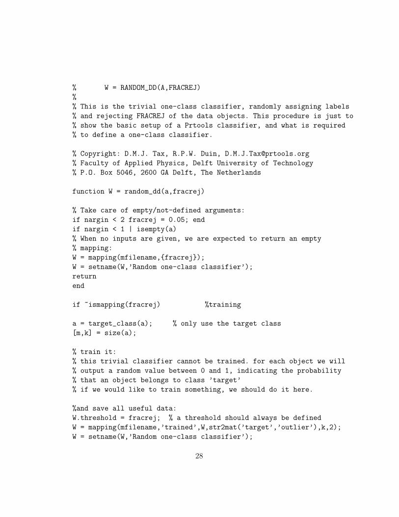
% W = RANDOM_DD(A,FRACREJ)

%

% This is the trivial one-class classifier, randomly assigning labels

% and rejecting FRACREJ of the data objects. This procedure is just to

% show the basic setup of a Prtools classifier, and what is required

% to define a one-class classifier.

% Copyright: D.M.J. Tax, R.P.W. Duin, D.M.J.Tax@prtools.org

% Faculty of Applied Physics, Delft University of Technology

% P.O. Box 5046, 2600 GA Delft, The Netherlands

function W = random_dd(a,fracrej)

% Take care of empty/not-defined arguments:

if nargin < 2 fracrej = 0.05; end

if nargin < 1 | isempty(a)

% When no inputs are given, we are expected to return an empty

% mapping:

W = mapping(mfilename,{fracrej});

W = setname(W,’Random one-class classifier’);

return

end

if ~ismapping(fracrej) %training

a = target_class(a); % only use the target class

[m,k] = size(a);

% train it:

% this trivial classifier cannot be trained. for each object we will

% output a random value between 0 and 1, indicating the probability

% that an object belongs to class ’target’

% if we would like to train something, we should do it here.

%and save all useful data:

W.threshold = fracrej; % a threshold should always be defined

W = mapping(mfilename,’trained’,W,str2mat(’target’,’outlier’),k,2);

W = setname(W,’Random one-class classifier’);

28

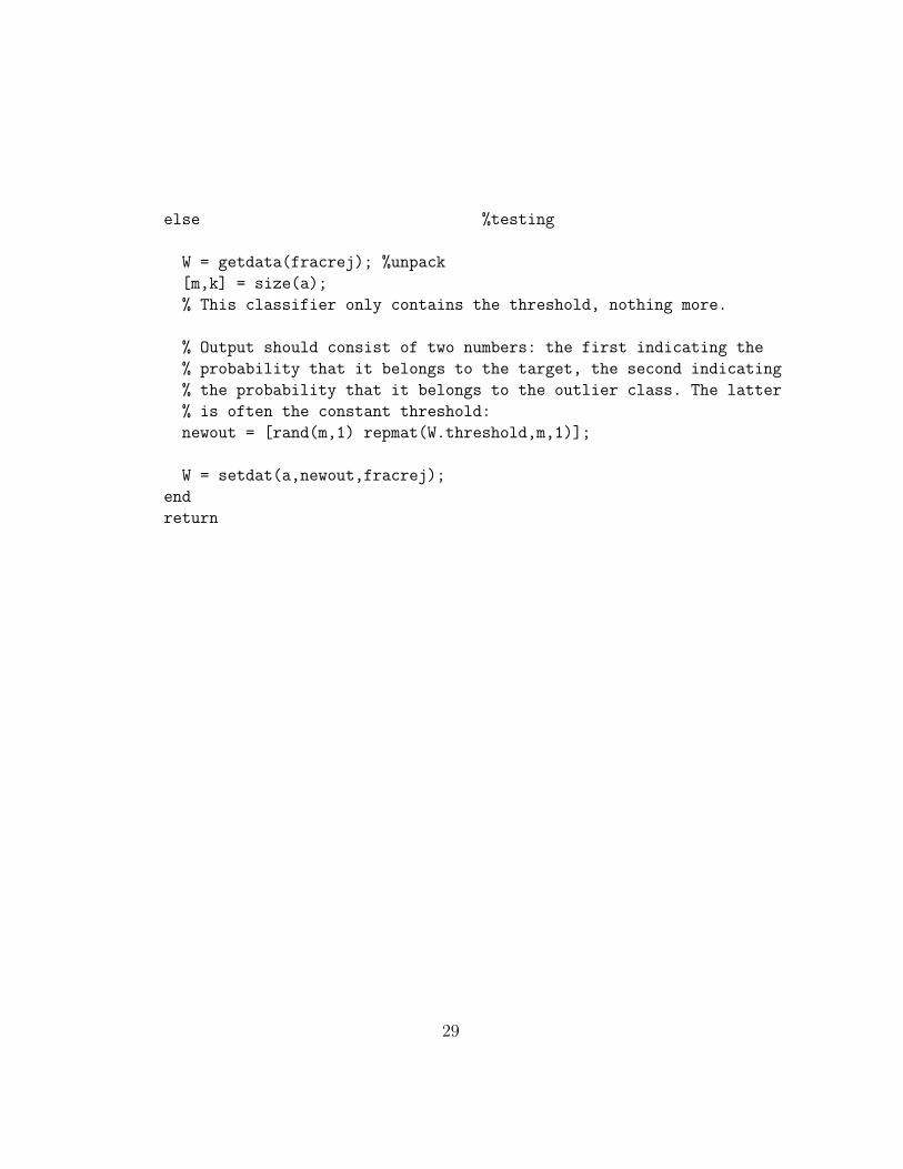
else %testing

W = getdata(fracrej); %unpack

[m,k] = size(a);

% This classifier only contains the threshold, nothing more.

% Output should consist of two numbers: the first indicating the

% probability that it belongs to the target, the second indicating

% the probability that it belongs to the outlier class. The latter

% is often the constant threshold:

newout = [rand(m,1) repmat(W.threshold,m,1)];

W = setdat(a,newout,fracrej);

end

return

29

Chapter 5

Error computation

5.1 Basic errors

In order to evaluate one-class classifiers, one has to find out what the errorof the first and second kind are (or the false positive and false negative rate).When you are only given target objects, life becomes hard and you cannotestimate these errors. But first assume you have some target and outlier testobjects available. The false positive and false negative rates can be computedby dd error:

>> x = target_class(gendatb([50 0]),’1’);

>> w = gauss_dd(x,0.1);

>> z = oc_set(gendatb(200),’1’);

>> e = dd_error(z,w)

>> dd_error(z*w) % other possibility

>> z*w*dd_error % other possibility

The first entry e(1) gives the false negative rate (i.e. the error on the targetclass) while e(2) gives the false positive rate (the error on the outlier class).Question: can you imagine what would happen when you would replaceoc set in the third line by target class?

5.2 Precision and recall

In the literature, two other measures are often used, namely

30

precision : defined as

precision =# of correct target predictions

# of target predictions,

recall : is basically the true positive rate

recall =# of correct target predictions

# of target examples.

These errors are returned in the second output variable of dd error:

>> [e,f] = dd_error(z,w)

Here f(1) contains the precision, and f(2) the recall.Finally, a derived performance criterion using the precision and recall is theF1 measure, defined as:

F1 =2 · precision · recall

precision + recall.

This can be computed using dd f1:

>> x = target_class(gendatb([50 0]),’1’);

>> w = svdd(x,0.1);

>> z = oc_set(gendatb(200),’1’);

>> dd_f1(x,w)

>> dd_f1(x*w)

>> x*w*dd_f1

5.3 Area under the ROC curve

In most cases we are not interested in just one single threshold (in the previ-ous example we took an error of 10% on the target class), we want to estimatethe whole ROC-curve. This can be estimated by dd roc:

>> x = target_class(gendatb([50 0]),’1’);

>> w = svdd(x,0.1,7);

>> z = oc_set(gendatb(200),’1’);

>> e = dd_roc(z,w)

>> e = dd_roc(z*w) % other possibility

>> e = z*w*dd_roc % other possibility

31

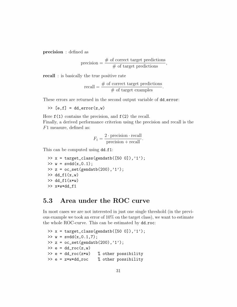
First the classifier is trained on x for a specific threshold. Then for varyingthresholds, the classifier is evaluated on dataset z. The results are returnedin a ROC curve, given in a matrix e with two columns, the first indicatingthe false negatives, the second the false positives.

0 0.1 0.2 0.3 0.4 0.5 0.6 0.7 0.8 0.9 10

0.1

0.2

0.3

0.4

0.5

0.6

0.7

0.8

0.9

1

outliers accepted (FP)

targ

ets

acce

pted

(T

P)

Figure 5.1: Receiver-Operating characteristic curve, wit the operating pointindicated by the dot.

The ROC-curve can be plotted by:

>> plotroc(e);

An example of such a ROC curve is shown in figure 5.1.In the newest version of the toolbox, the ROC is extended to show also theoperating point of the classifier. When this feature is required, you have tosupply the mapping and the dataset separately:

>> a = oc_set(gendatb,1);

>> w = gauss_dd(a,0.1);

>> h = plotroc(w,a)

By moving the mouse, and clicking, the user can change the position of theoperating point. Inside the figure, a new mapping with this new operatingpoint is stored. This mapping can be retrieved in the Matlab working spaceby:

>> w2 = getrocw(h)

To get a feeling for this, please try the demo dd ex8.

32

Because it is very hard to compare ROC curves of different classifiers, oftenthe AUC error (Area Under the AUC curve is taken). In my definition ofthe AUC error, the larger the value, the better the one-class classifier. It iscomputed from the ROC curve values using the function dd auc:

>> x = target_class(gendatb([50 0]),’1’);

>> w = svdd;

>> z = oc_set(gendatb(200),’1’);

>> e = dd_roc(z,w);

>> err = dd_auc(e);

In many cases only a restricted range for the false negatives is of interest:for instance, we want to reject less than half of the target objects. In thesecases one may want to set bounds on the range of the AUC error:

>> e = dd_roc(z,w);

>> err = dd_auc(e,[0.05 0.5]);

Analogous to the ROC curve, also a precision-recall graph can be computed.This curve shows how the precision depends on the recall. This is imple-mented by the function dd prc”

>> b = oc_set(gendatb);

>> w = gauss_dd(b);

>> r = dd_prc(b,w);

>> plotroc(r)

Furthermore, it is possible to convert the ROC curve to a precision-recallcurve using roc2prc.m.Identical to the Area under the ROC curve, the mean precision (or the aver-age precision) can be defined, which basically computes the area under theprecision-recall curve:

>> e = dd_meanprec(r)

A more extensive example is shown in dd ex12.m.

33

0 0.1 0.2 0.3 0.4 0.5 0.6 0.7 0.8 0.9 10

0.05

0.1

0.15

0.2

0.25

0.3

0.35

0.4

0.45

0.5

Probability cost function

Nor

mal

ized

exp

ecte

d co

st

Figure 5.2: The cost curve derived from the same dataset and classifier as inFigure 5.1.

5.4 Cost curve

Another proposal for plotting the performance of a classifier is by using thecost-curve [DH00]. As you can see in figure 5.1, there are many thresholdsthat are suboptimal: there is often another operating point for which at leastone of the errors is lower. For instance, the operating point FP = 0.38, TP =0.72 is suboptimal, because operating point FP = 0.38, TP = 0.92 has muchbetter true positive rate with equal false positive rate. For a relative largerange of misclassification costs the operating point FP = 0.38, TP = 0.92will be the optimal one.This is indicated in a cost curve. For a varying cost-ratio between the twoclasses, the (normalized) expected cost is computed. Each operating pointappears as a line in this plot. In Figure 5.2 the cost curve for the same datasetand classifier as of the ROC curve in Figure 5.1 is shown. The operating pointof Figure 5.1 is indicated by the dotted line in Figure 5.2. The combinationof operating points that form the lower hull is indicated by the thick line,and shows the best operating points over the range of costs. This cost curveis obtained like:

>> a = oc_set(gendatb,1);

>> w = gauss_dd(a,0.1);

>> c = a*w*dd_costc;

>> plotcostc(c)

For more information, please look at [DH00].

34

5.5 Generating artificial outliers

When you are not so fortunate to have example outliers available for testing,you can create them yourself. Say that z is a set of test target objects.Artificial outliers can be generated by:

>> z_o = gendatblockout(z,100)

This creates a new dataset from z, containing both the target objects from z

and 100 new artificial outliers. The outliers are drawn from a block-shapeduniform distribution that covers the target objects in z. (An alternative isto draw samples not from a box, but from a Gaussian distribution. This isimplemented by gendatoutg.)This works well in practice for low dimensional dataset. For higher dimen-sions, it becomes very inefficient. Most of the data will be in the ’corners’ ofthe box. In these cases it is better to generate data uniform in a sphere.

>> z_o = gendatout(z,100)

In this version, the most tight hypersphere around the data is fitted. Giventhe center and radius of this sphere, data can be uniformly generated byrandsph (this is not trivial!).For (very) high dimensional feature spaces there is still another method togenerate outliers, gendatouts. This method first estimates the PCA sub-space in which the target data is distributed, then it will generate outliers inthis subspace. The outliers are drawn from a sphere again.

5.6 Cross-validation

The toolbox has an extra procedure to facilitate cross-validation. In cross-validation a dataset is split into B batches. From these batches B − 1 areused to train a classifier, and the left-out batch is used to evaluate it. Thisis repeated B times, and the performances are averaged. The advantage isthat given a limited training set, it is still possible to obtain a relatively goodclassifier, and estimate its performance on an independent set.In practice, this cross-validation procedure is applied over and over again.Not only to evaluate and compare the performance of classifiers, but also tooptimize hyperparameters. To keep the procedure as flexible as possible, thecross-validation is kept as simple as possible. An index vector is generated

35

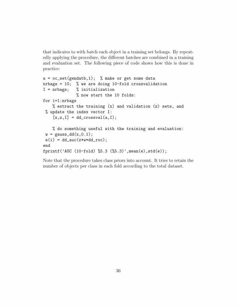
that indicates to with batch each object in a training set belongs. By repeat-edly applying the procedure, the different batches are combined in a trainingand evaluation set. The following piece of code shows how this is done inpractice:

a = oc_set(gendatb,1); % make or get some data

nrbags = 10; % we are doing 10-fold crossvalidation

I = nrbags; % initialization

% now start the 10 folds:

for i=1:nrbags

% extract the training (x) and validation (z) sets, and

% update the index vector I:

[x,z,I] = dd_crossval(a,I);

% do something useful with the training and evaluation:

w = gauss_dd(x,0.1);

e(i) = dd_auc(z*w*dd_roc);

end

fprintf(’AUC (10-fold) %5.3 (%5.3)’,mean(e),std(e));

Note that the procedure takes class priors into account. It tries to retain thenumber of objects per class in each fold according to the total dataset.

36

Chapter 6

General remarks

In this chapter I collected some remarks which are important to see once,but did not fit in the line of the previous chapters.

1. If you want to know more about a classifier or function, always try thehelp command.

2. Also have a look at the file Contents.m. This contains the full list offunctions and classifiers defined in the toolbox.

3. In older versions of the toolbox, the width parameter σ in the sup-port vector data description was optimized automatically. This wasdone such that a prespecified fraction fracrej of the objects was onthe boundary (so these are support vectors with 0 < αi < 1/(Nν)).Another parameter C was set such that another prespecified fractionfracerr of objects was outside the boundary (the support vectors withαi = 1/(Nν)). The default of this fraction was fracerr = 0.01 andwas often ignored in practical experiments. But this lead sometimes topoor results, and created a lot of confusion. If you really want to, andif you’re lucky that I included it, it is still available under newsvdd.m.

I decided to consider the parameter σ as a hyper-parameter. Thisparameter will not be optimized automatically, but has to be set bythe user. To obtain the prespecified error fracrej on the target set,the parameter C will be set. The parameter fracerr is removed.

Another complaint about the first implementation of the svdd was,that it was completely aimed at the RBF kernel. That was because the

37

optimization simplifies significantly with this assumption. Using ksvdd

or incsvdd this restriction is now lifted. In particular incsvdd is rec-ommended because it does not rely on external quadratic programmingoptimizers which always creates problems.

4. There is also a set of functions for visualizing the output of a classifierin 2D. (Note: there is no obvious way to clearly visualize a classifier inmore than 2 dimensions, and it is therefore not defined.) One can definea grid of objects around a 2D dataset, and put that into a dataset. Thatdataset can be classified by the classifier, and mapped back into thefeature space. The user can thus inspect the output of the classifier forthe whole feature space around the target class.

This is explicitly done in the following code:

>> x = target_class(gendatb([50 0]),’1’);

>> w = svdd(x,0.1,5);

>> scatterd(x);

>> griddat = gendatgrid;

>> out = griddat*w;

>> plotg(griddat,out);

>> hold on;

>> scatterd(x);

5. There is also one function which is in essence not a one-class classifier,but a preprocessor: the kernel whitening kwhiten. This mapping doesnot classify data, only transforms it into a new dataset. It is hoped thatit is transformed into a shaped which can be described better by one-class classifiers. The easiest way to work with this type of preprocessing,is to exploit some Prtools techniques:

>> x = target_class(gendatb([50 0]),’1’);

>> w_kpca = kwhiten(x,0.99,’p’,2);

>> w = gauss_dd(x*w_kpca,0.1);

>> W = w_kpca*w;

This W can now be used as a normal classifier.

38

6. I’m not responsible for the correct functioning of the toolbox, but ofcourse I do my best to make the toolbox as useful and bug-free as possi-ble. Please email me when you have found a bug at D.M.J.Tax@prtools.org.I’m also very interested when people have defined new one-class classi-fiers.

39

Chapter 7

Contents.m of the toolbox

% Data Description Toolbox

% Version 2.0.0 23-Jul-2013

%

%Dataset construction

%--------------------

%isocset true if dataset is one-class dataset

%gendatoc generate a one-class dataset from two data matrices

%oc_set change normal classif. problem to one-class problem

%target_class extracts the target class from an one-class dataset

%gendatgrid create a grid dataset around a 2D dataset

%gendatout create outlier data in a hypersphere around the

% target data

%gendatblockout create outlier data in a box around the target class

%gendatoutg create outlier data normally distributed around the

% target data

%gendatouts create outlier data in the data PCA subspace in a

% hypersphere around the target data

%gendatkriegel artificial data according to Kriegel

%dd_crossval cross-validation dataset creation

%dd_looxval leave-one-out cross-validation dataset creation

%dd_label put the classification labels in the same dataset

%

%Data preprocessing

%------------------

%dd_proxm replacement for proxm.m

40

%kwhiten rescale data to unit variance in kernel space

%gower compute the Gower similarities

%

%One-class classifiers

%---------------------

%random_dd description which randomly assigns labels

%stump_dd threshold the first feature

%gauss_dd data description using normal density

%rob_gauss_dd robustified gaussian distribution

%mcd_gauss_dd Minimum Covariance Determinant gaussian

%mog_dd mixture of Gaussians data description

%mog_extend extend a Mixture of Gaussians data description

%parzen_dd Parzen density data description

%nparzen_dd Naive Parzen density data description

%

%autoenc_dd auto-encoder neural network data description

%kcenter_dd k-center data description

%kmeans_dd k-means data description

%pca_dd principal component data description

%som_dd Self-Organizing Map data description

%mst_dd minimum spanning tree data description

%

%nndd nearest neighbor based data description

%knndd K-nearest neighbor data description

%ball_dd L_p-ball data description

%lpball_dd extended L_p-ball data description

%svdd Support vector data description

%incsvdd Incremental Support vector data description

%(incsvc incremental support vector classifier)

%ksvdd SVDD on general kernel matrices

%lpdd linear programming data description

%mpm_dd minimax probability machine data description

%lofdd local outlier fraction data description

%lofrangedd local outlier fraction over a range

%locidd local correlation integral data description

%abof_dd angle-based outlier fraction data description

%

%dkcenter_dd distance k-center data description

41

%dnndd distance nearest neighbor based data description

%dknndd distance K-nearest neighbor data description

%dlpdd distance-linear programming data description

%dlpsdd distance-linear progr. similarity description

%

%isocc true if classifier is one-class classifier

%

%AUC optimizers

%--------------

%rankboostc Rank-boosting algorithm

%auclpm AUC linear programming mapping

%

%Classifier postprocessing/optimization/combining.

%--------------------------------------

%consistent_occ optimize the hyperparameter using consistency

%optim_auc optimize the hyperparameter by maximizing AUC

%dd_normc normalize oc-classifier output

%multic construct a multi-class classifier from OCC’s

%ocmcc one-class and multiclass classifier sequence

%

%Error computation.

%-----------------

%dd_error false positive and negative fraction of classifier

%dd_confmat confusion matrix

%dd_kappa Cohen’s kappa coefficient

%dd_f1 F1 score computation

%dd_eer equal error rate

%dd_roc computation of the Receiver-Operating Characterisic curve

%dd_prc computation of the Precision-Recall curve

%dd_auc error under the ROC curve

%dd_meanprec mean precision of the Precision-Recall curve

%dd_costc cost curve

%dd_aucostc area under the cost curve

%dd_delta_aic AIC error for density estimators

%dd_fp compute false positives for given false negative

% fraction

%simpleroc basic ROC curve computation

%dd_setfn set the threshold for a false negative rate

42

%roc2prc convert ROC to precision-recall curve

%

%Plot functions.

%--------------

%plotroc plot an ROC curve or precision-recall curve

%plotcostc plot the cost curve

%plotg plot a 2D grid of function values

%plotw plot a 2D real-valued output of classifier w

%askerplot plot the FP and FN fraction wrt the thresholds

%plot_mst plot the minimum spanning tree

%lociplot plot a lociplot

%

%Support functions.

%-----------------

%dd_version current version of dd_tools, with upgrade possibility

%istarget true if an object is target

%find_target gives the indices of target and outlier objs from a dataset

%getoclab returns numeric labels (+1/-1)

%dist2dens map distance to posterior probabilities

%dd_threshold give percentiles for a sample

%randsph create outlier data uniformly in a unit hypersphere

%makegriddat auxiliary function for constructing grid data

%relabel relabel a dataset

%dd_kernel general kernel definitions

%center center the kernel matrix in kernel space

%gausspdf multi-variate Gaussian prob.dens.function

%mahaldist Mahalanobis distance

%sqeucldistm square Euclidean distance

%mog_init initialize a Mixture of Gaussians

%mog_P probability density of Mixture of Gaussians

%mog_update update a MoG using EM

%mogEMupdate EM procedure to optimize Mixture of Gaussians

%mogEMextend smartly extend a MoG and apply EM

%mykmeans own implementation of the k-means clustering algorithm

%getfeattype find the nominal and continuous features

%knn_optk optimization of k for the knndd using leave-one-out

%volsphere compute the volume of a hypersphere

%scale_range compute a reasonable range of scales for a dataset

43

%nndist_range compute the average nearest neighbor distance

%inc_setup startup function incsvdd

%inc_add add one object to an incsvdd

%inc_remove remove one object from an incsvdd

%inc_store store the structure obtained from inc_add to prtools mapping

%unrandomize unrandomize objects for incsvc

%plotroc_update support function for plotroc

%roc_hull convex hull over a ROC curve

%lpball_dist lp-distance to a center

%lpball_vol volume of a lpball

%lpdist fast lp-distance between two datasets

%nndist (average) nearest neighbor distance

%dd_message printf with colors

%

%Examples

%--------

%dd_ex1 show performance of nndd and svdd

%dd_ex2 show the performances of a list of classifiers

%dd_ex3 shows the use of the svdd and ksvdd

%dd_ex4 optimizes a hyperparameter using consistent_occ

%dd_ex5 shows the construction of lpdd from dlpdd

%dd_ex6 shows the different Mixture of Gaussians classifiers

%dd_ex7 shows the combination of one-class classifiers

%dd_ex8 shows the interactive adjustment of the operating point

%dd_ex9 shows the use of dd_crossval

%dd_ex10 shows the use of the incremental SVDD

%dd_ex11 the construction of a multi-class classifier using OCCs

%dd_ex12 the precision-recall-curve and the ROC curve

%dd_ex13 kernelizing the AUCLPM

%dd_ex14 show the combination of a one-class and multi-class

%dd_ex15 show the parameter optimization mapping

%

% Copyright: D.M.J. Tax, D.M.J.Tax@prtools.org

% Faculty EWI, Delft University of Technology

% P.O. Box 5031, 2600 GA Delft, The Netherlands

44

Index

artificial outliers, 34AUC, 9, 30

classifiercreating, 15define it yourself, 26inspecting, 16trivial, 26visualizing, 37

classifier output, 14classifiers, 17

multi-class, 25combining classifiers, 24confidence, 26cost curve, 33cross-validation, 34

datasetinspecting, 12

datasets, 10creating, 10

dd auc, 32dd error, 29dd F1, 30dd roc, 30density based classifiers, 24distance based classifiers, 24

error, 7, 29

F1, 30false negative, 7, 15

false positive, 7

gauss dd, 15gendatblockout, 34gendatgrid, 37gendatoc, 10gendatout, 34

help, 36

isocset, 12

kwhiten, 37

label as outlier, 10label as target, 12

mean precision, 32mog dd, 17multi-class classifiers, 25

normalization of classifiers, 24

oc set, 11One-class classification, 6operating point, 30, 31, 33outlier

generating, 34outlier class, 6outliers, 15output of a classifier, 26

philosophy, 4

45

plotg, 37precision, 30precision-recall curve, 32Prtools, 4

random dd, 26recall, 30relabel, 13ROC curve, 8, 30

svdd, 16, 30, 36

target class, 6target class, 12threshold, 15true negative, 7true positive, 7

46

Bibliography

[Bis95] C.M. Bishop. Neural Networks for Pattern Recognition. OxfordUniversity Press, Walton Street, Oxford OX2 6DP, 1995.

[DH00] C. Drummond and R.C. Holte. Explicitly representing expectedcost: an alternative to ROC representation. In Knowledge Discov-ery and Data Mining, pages 198–207, 2000.

[LEGJ03] G.R.G. Lanckriet, L. El Ghaoui, and M.I. Jordan. Robust nov-elty detection with single-class mpm. In S. Becker, S. Thrun, andK. Obermayer, editors, Advances in Neural Information Process-ing Systems, volume 15. MIT Press: Cambridge, MA, 2003. E,.

[PTD03] E. Pekalska, D.M.J. Tax, and R.P.W. Duin. One-class LP classi-fier for dissimilarity representations. In S. Becker, S. Thrun, andK. Obermayer, editors, Advances in Neural Information Process-ing Systems, volume 15. MIT Press: Cambridge, MA, 2003.

[RVD99] P.J. Rousseeuw and K. Van Driessen. A fast algorithm for the min-imum covariance determinant estimator. Technometrics, 41:212–223, 1999.

[Tax01] D.M.J. Tax. One-class classification. PhD thesis, Delft Universityof Technology, http://ict.ewi.tudelft.nl/˜davidt/thesis.pdf, June2001.

[TM03] D.M.J. Tax and K.R. Muller. Feature extraction for one-classclassification. In Proceedings of the ICANN/ICONIP 2003, pages342–349, 2003.

[YD98] A. Ypma and R.P.W. Duin. Support objects for domain approxi-mation. In ICANN’98, Skovde (Sweden), September 1998.

47