data imaging. the history of the data image first proposed as part of the seminal parallel...
Post on 18-Dec-2015
218 views
TRANSCRIPT

Data Imaging
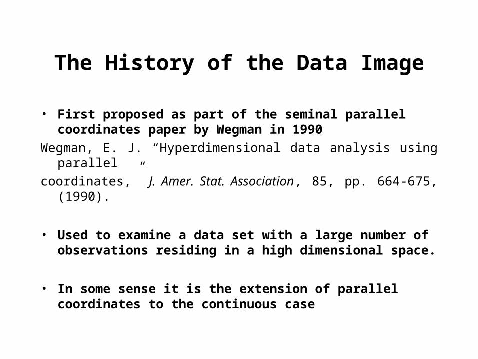
The History of the Data Image
• First proposed as part of the seminal parallel coordinates paper by Wegman in 1990
Wegman, E. J. “Hyperdimensional data analysis using parallel
coordinates,” J. Amer. Stat. Association, 85, pp. 664-675, (1990).
• Used to examine a data set with a large number of observations residing in a high dimensional space.
• In some sense it is the extension of parallel coordinates to the continuous case

Recent Reinvestigation of Data Imaging
• Recent work of Minnotte and West have examined the marriage of clustering schemes and data imaging
• The idea is for the user to identify underlying high-dimensional cluster structure visually
• "The data image: a tool for exploring high dimensional data sets," Michael C. Minnotte and R. Webster West, 1999. 1998 Proceedings of the ASA Section on Statistical Graphics, in press.
• Minnottee, West, and Solka are preparing a JCGS submission on data imaging
Issues Associated with the Minnotte/West Data Imaging Method
• These are the usual clustering isssues.
• Shall we scale the data first?
• How shall we compute distances between observations?
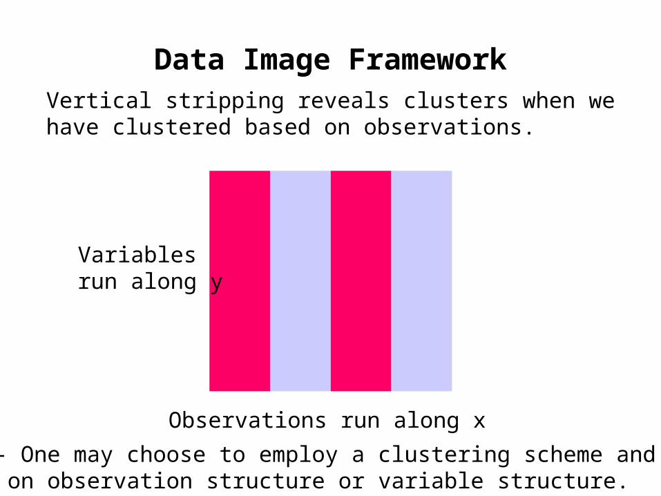
Data Image Framework
Variablesrun along y
Observations run along x
Vertical stripping reveals clusters when we have clustered based on observations.
N.B. - One may choose to employ a clustering scheme and sort based on observation structure or variable structure.
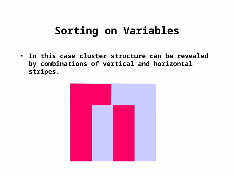
Sorting on Variables
• In this case cluster structure can be revealed by combinations of vertical and horizontal stripes.

Splus Data Image Code
• Mike Minnotte has been kind enough to provide us with a version of the data imaging code for our enjoyment.
• It runs quite well under S-Plus on the PC but I have yet been able to make it go under R.
• There are numerous straight forward extensions that would be fun to do with the code.

Dataimage -I
• dataimage<-function(data,obs.sort="complete",var.sort="complete",std=T, obs.met="euclidean",var.met="euclidean",doplot=T, maxv=apply(data,2,max),minv=apply(data,2,min),var.l=T,obs.l=T, lab.l=dimnames(data)[[2]],lab.r=dimnames(data)[[2]], lab.t=dimnames(data)[[1]],lab.b=dimnames(data)[[1]])
• {# calculate (and optionally plot) sortings for dataimage (color histogram)• # data - matrix or data frame of observations (rows) and variables (columns)• # obs.sort - method of sorting observations. One of:# "none" - leave in original ordering• # "complete" - heirarchical clustering, where cluster distances are• # measured as max of point distances# "single" - heirarchical clustering, where
cluster distances are# measured as min of point distances# "average" - heirarchical clustering, where cluster distances are# measured as average of point distances# "farthest" - farthest insertion spanning tour# "nearest" - nearest insertion spanning tour# k (numeric) - sort on variable k# var.sort - method of sorting variables, as obs.sort# std - if T, standardize all variables before sorting# obs.met - distance metric for observations. One of:# "euclidean" - L2# "manhattan" - L1# "maximum" - L-Infinity# var.met - distance metric for variables, as obs.met# doplot - if T, plot data image. If false, return list consisting of# obs.ord: vector of observation orderings# var.ord: vector of variable orderings# data: original data matrix# maxv - vector of maximums for each variable# minv - vector of minimums for each variable# maxv, minv may be passed to keep color scale the same between images# var.l - if T, label variables in plot# obs.l - if T, label observations in plot# lab.l - character vector for variable labels (left side)# lab.r - character vector for variable labels (right side)# lab.t - character vector for observation labels (top)# lab.b - character vector for observation labels (bottom)
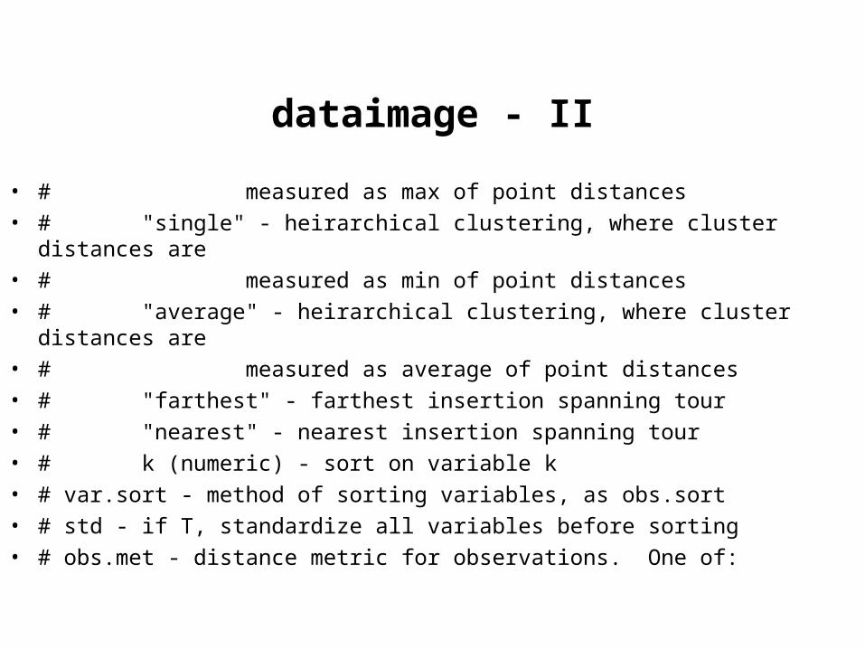
dataimage - II
• # measured as max of point distances• # "single" - heirarchical clustering, where cluster
distances are• # measured as min of point distances• # "average" - heirarchical clustering, where cluster
distances are• # measured as average of point distances• # "farthest" - farthest insertion spanning tour• # "nearest" - nearest insertion spanning tour• # k (numeric) - sort on variable k• # var.sort - method of sorting variables, as obs.sort• # std - if T, standardize all variables before sorting• # obs.met - distance metric for observations. One of:

dataimage - III
• # "euclidean" - L2• # "manhattan" - L1• # "maximum" - L-Infinity# var.met - distance
metric for variables, as obs.met• # doplot - if T, plot data image. If false, return
list consisting of• # obs.ord: vector of observation orderings• # var.ord: vector of variable orderings• # data: original data matrix• # maxv - vector of maximums for each variable# minv
- vector of minimums for each variable• # maxv, minv may be passed to keep color scale
the same between images
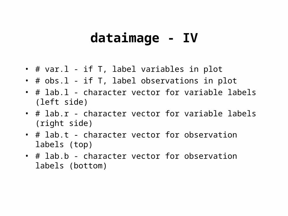
dataimage - IV
• # var.l - if T, label variables in plot• # obs.l - if T, label observations in plot• # lab.l - character vector for variable labels
(left side)• # lab.r - character vector for variable labels
(right side)• # lab.t - character vector for observation
labels (top)• # lab.b - character vector for observation
labels (bottom)
Artificial Olfactory Systems
[1] - T. A. Dickinson, S. R. Johnson, H. E. McClelland, P. C. Jurs, J. White, J.S. Kauer, and D. R. Walt (1998), "Mixture Component Identification UsingMultiple Wavelength Monitoring oa an Optical Sensor Array and ComputationalNeural Networks," preprint (submitted for publication).
[2] T. A. Dickinson, J. White, J. S. Kauer, and D. R. Walt (1996), "AChemica-Detecting System Based on a Cross-REactive Optical Sensor Array," Nture,Vol. 382, pp. 697-700.

Types of Artificial Noses
• There are fiber optic based systems (Tufts/Walt)
• There are electronic ones (Cal Tech/Nate Lewis)
Why Build Artificial Noses
• Explosives detection
• Drug detection
• Ground water contamination detection
• Human detection

Basics of the Fiber Optic Nose
• Consists of 19 doped fibers
• An analyte (mixture of compounds) is passed across the fibers and the resultant times series is sampled 60 times
• The system is typically measured at two wavelengths
• 620 nm and 690 nm
• Response of the system to a particular analyte consists of a point in R^(2x19x60) dimensional space

Ground Water Contamination Problem
• The compounds that were used as part of the artificial olfactory study include air, trichloroethylene (the target compound), benzene, BTEX (a mixture of benzene, toluene, ethylbenzene, and xylene), carbon tetrachloride, chlorobenzene, chloroform, kerosene,1-octane, and Coleman fuel.

Data Image of Fiber 12 Activity

Intrusion Detection
• NSWCDD has developed a network based intrusion detection package called SHADOW
• Work is ongoing at NSWCDD to improve this capabilities of this package
• I have been examining the application of data imaging to this problem

Machine Ports
• Each machine that is on the internet has a certain number of ports that are used by the machine to handle internet traffic
• Many of these ports are well known and preconfigued to allow certain services
• 21 is usually set for ftp services
• The activity on the ports of the machine conveys information about the nature of the machine
Port Probability Matrix
• We have assembled a data set that represents the probability of access a particular port for a set of 993 machines at our center.
• We recorded the probability of accessing any of 668 ports on each machine.
• We are currently studying the use of data imaging as a means to reveal cluster structure in this probability matrix
• Cluster structure may allow the user to infer useful information about the inherent functions of the various machines


Data Image of Gene Expression Data With Scaling, Sorting on Observations, and No Sorting on Variables.
GFAP
MOG
GRb2
L1
5HT2
NOS
mGluR3
NMDA2B
nAChRa3
5HT1b
NMDA2C
5HT1c
bFGF
ChAT
aFGF
cfos
G67I86
trk
mGluR1
NMDA2A
nAChRe
nAChRd
Ins1
nAChRa2
mGluR4
nAChRa6
PDGFb
IP3R3
mGluR2
5HT3
mGluR8
mGluR6
mAChR3
mAChR4
SC6
GDNF
NGF
PDGFR
keratin
cjun
nAChRa5
nAChRa4
BDNF
NMDA2D
EGF
CNTF
IP3R1
FGFR
TH
Brm
IGF II
TGFR
InsR
SC7
CCO2
CCO1
cyclin A
PTN
MK2
SC1
GAP43
DD63.2
ODC
H2AZ
CRAF
NT3
cyclin B
IGFR1
CNTFR
TCP
IGF I
PDGFa
SOD
Ins2
IGFR2
NFH
GRb1
GRg3
GRa5
GRa2
synaptophysin
MAP2
neno
GRb3
GRa3
IP3R2
GRa1
trkC
statin
pre-GAD67
GRa4
mGluR7
S100 beta
G67I80/86
trkB
GRg2
GAD65
ACHE
mAChR2
GAD67
mGluR5
nAChRa7
EGFR
SC2
GAT1
nestin
cellubrevin
actin
NFL
NMDA1
GRg1
NFM
E11
E13
E15
E18
E21
P0
P7
P14
A
E11
E13
E15
E18
E21
P0
P7
P14
A
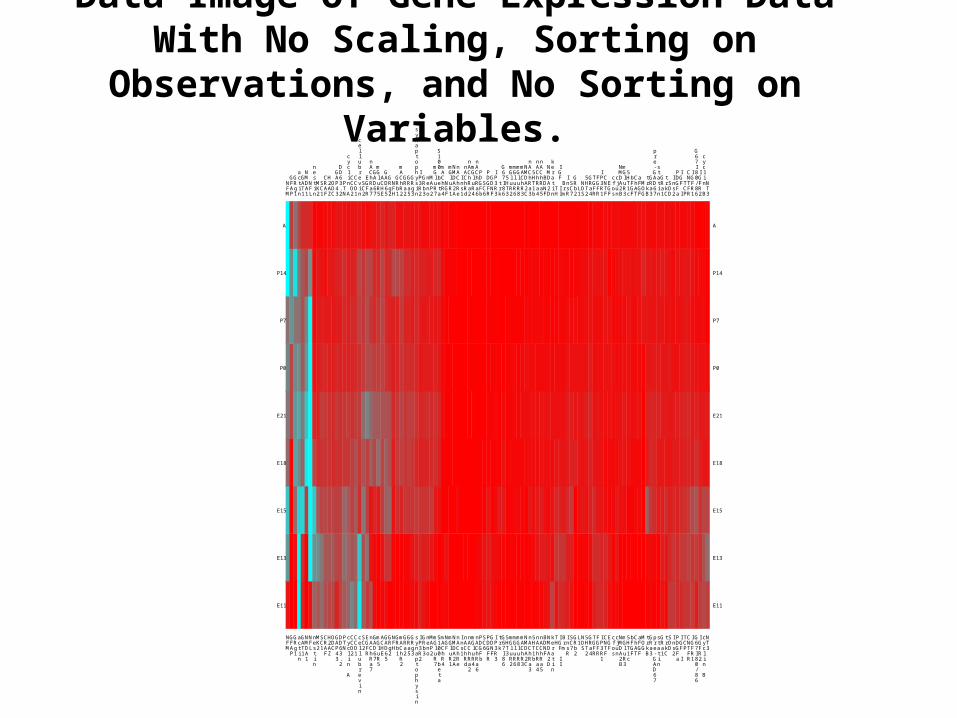
Data Image of Gene Expression Data With No Scaling, Sorting on Observations, and No Sorting
on Variables.
NFM
GFAP
GRg1
actin
GAT1
NMDA1
NFL
nestin
MK2
SC1
CRAF
H2AZ
ODC
GAP43
DD63.2
PTN
cyclin A
CCO2
CCO1
cellubrevin
SC2
EGFR
nAChRa7
GAD67
mGluR5
ACHE
GAD65
GRg2
NFH
GRb1
mAChR2
GRa2
GRa5
GRg3
synaptophysin
IP3R2
GRb3
neno
MAP2
mGluR7
S100 beta
mAChR4
NGF
mGluR1
NMDA2A
nAChRe
Ins1
nAChRd
nAChRa2
mGluR4
nAChRa6
PDGFb
SC6
PDGFR
GDNF
IP3R3
trk
G67I86
5HT3
mGluR2
mGluR6
mGluR8
mAChR3
NMDA2C
nAChRa3
5HT1b
nAChRa4
nAChRa5
BDNF
NMDA2D
keratin
TH
IGF II
Brm
InsR
SC7
GRb2
L1
NOS
5HT2
GRa4
TGFR
FGFR
IP3R1
CNTF
EGF
cfos
cjun
NMDA2B
mGluR3
5HT1c
bFGF
ChAT
aFGF
MOG
trkB
GRa3
pre-GAD67
statin
GRa1
trkC
SOD
Ins2
PDGFa
IGF I
TCP
CNTFR
IGFR1
G67I80/86
IGFR2
cyclin B
NT3
E11
E13
E15
E18
E21
P0
P7
P14
A
E11
E13
E15
E18
E21
P0
P7
P14
A