data loading complete.ppt - cgg · 2015-03-11 · introduction data loading has been made much...
TRANSCRIPT

SAMPLE IMAGE
Data Loading in CE8
Simon VoiseyJune 2008Hampson-Russell LondonWritten for CE8R1
Introduction
Data loading has been made much easier in CE8. The principles and locations of the buttons remain the same however in theand locations of the buttons remain the same, however in the case of 2D data there is no need to formulate your own geometry.
Data loading is rarely a fun task, so I hope this document makes life a little easier.
2
Sections
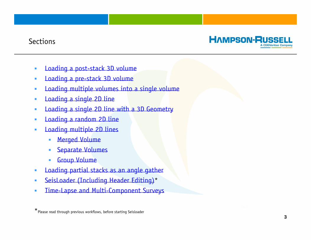
Loading a post-stack 3D volumeLoading a pre-stack 3D volumeLoading multiple volumes into a single volume Loading a single 2D lineLoading a single 2D line with a 3D GeometryLoading a random 2D lineLoading multiple 2D lines
Merged VolumeSeparate VolumesGroup Volume
Loading partial stacks as an angle gatherSeisLoader (Including Header Editing)*Time-Lapse and Multi-Component Surveys
3*Please read through previous workflows, before starting Seisloader
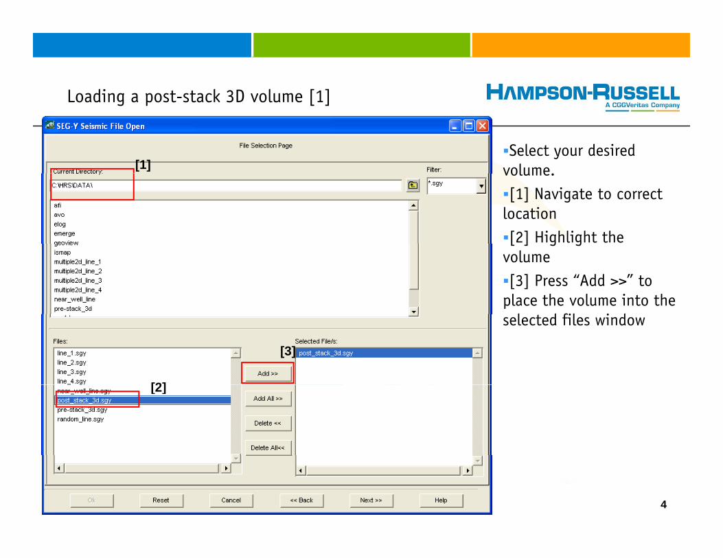
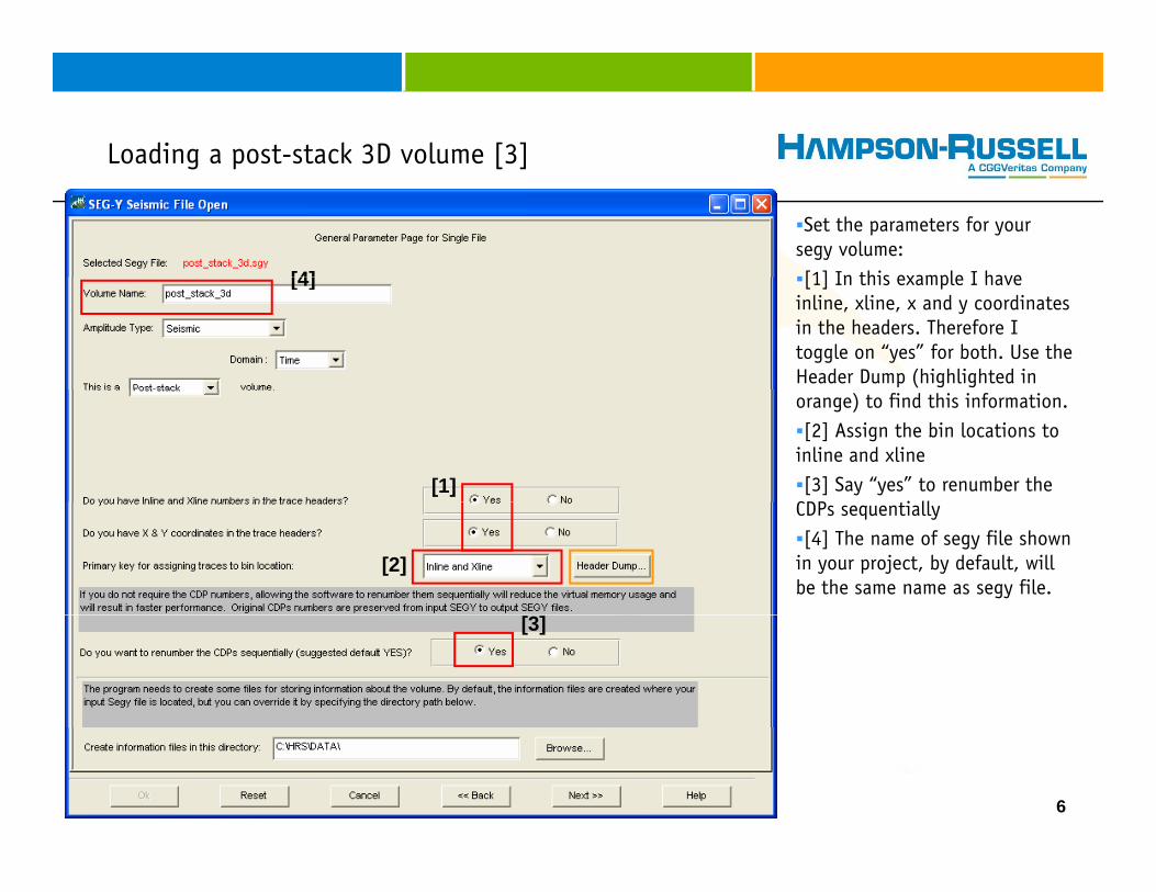
Loading a post-stack 3D volume [1]g p [ ]
Select your desired volume.[1] volume. [1] Navigate to correct
location[2] Highlight the [ ] g g
volume[3] Press “Add >>” to
place the volume into the l d fil i dselected files window
[2]
[3]
[2]
4
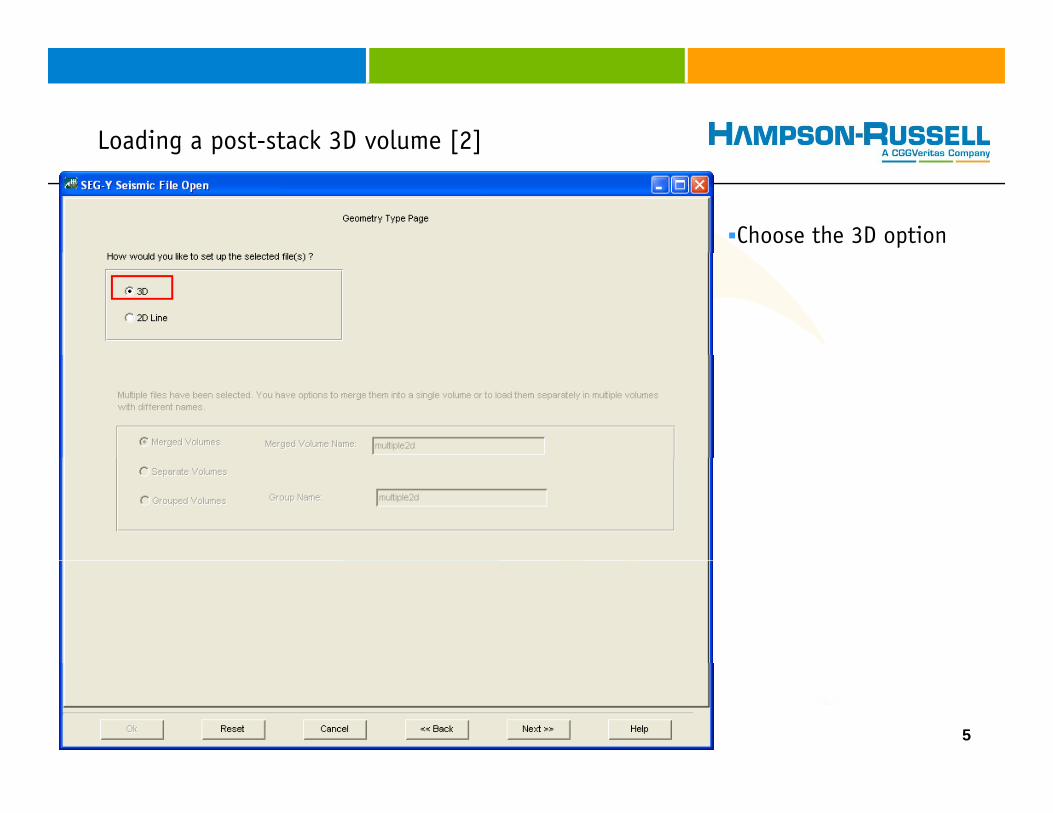
Loading a post-stack 3D volume [2]g p [ ]
Choose the 3D option
5
Loading a post-stack 3D volume [3]g p [ ]
Set the parameters for your segy volume:[1] In this example I have[4] [1] In this example I have
inline, xline, x and y coordinates in the headers. Therefore I toggle on “yes” for both. Use the Header Dump (highlighted in
[4]
orange) to find this information.[2] Assign the bin locations to
inline and xline[3] Say “yes” to renumber the
CDP ti ll[1]
CDPs sequentially[4] The name of segy file shown
in your project, by default, will be the same name as segy file.
[2]
[3]
6
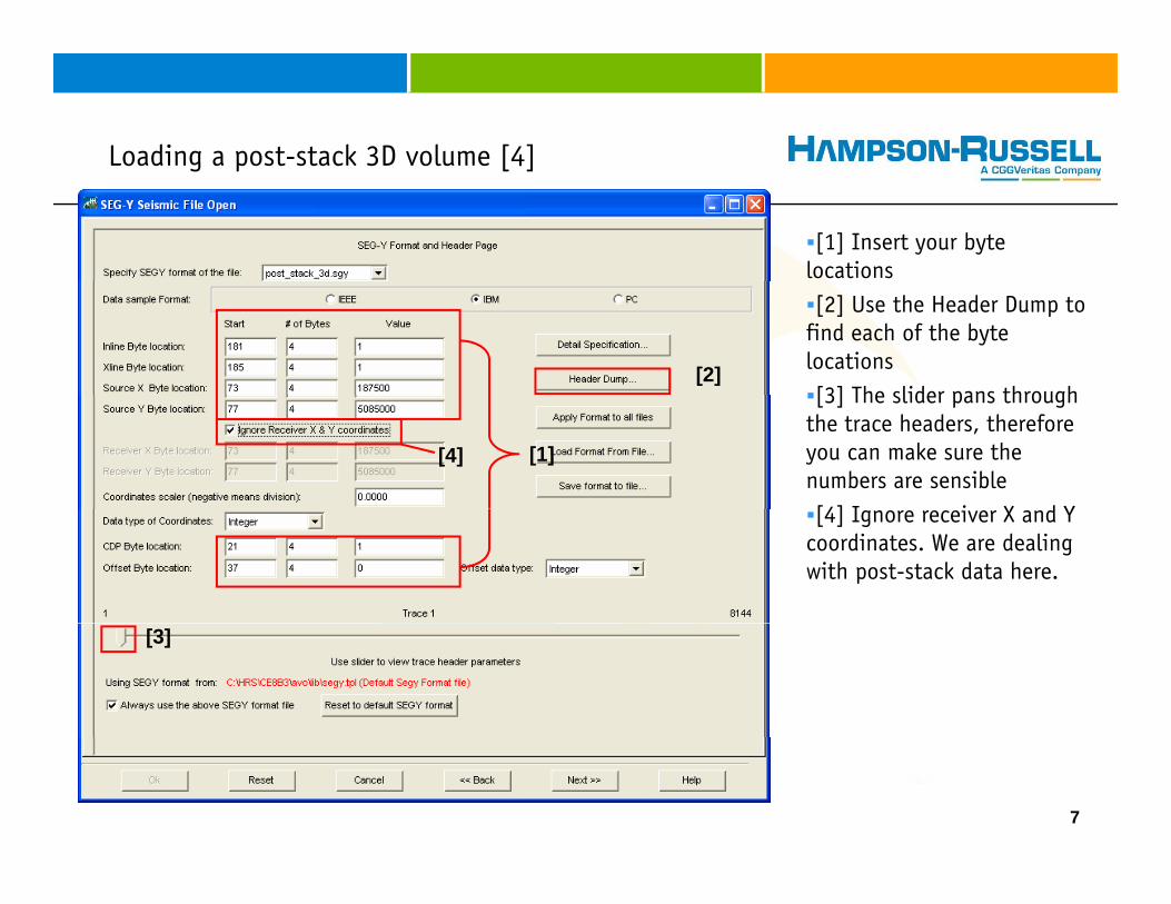
Loading a post-stack 3D volume [4]g p [ ]
[1] Insert your byte locations[2] Use the Header Dump to
find each of the byte locations[3] The slider pans through
[2][3] The slider pans through
the trace headers, therefore you can make sure the numbers are sensible[4] I i X d Y
[1][4]
[4] Ignore receiver X and Y coordinates. We are dealing with post-stack data here.
[3]
7

Loading a post-stack 3D volume [5]g p [ ]
Scanning the seismic is an important step. The software defines the location of the traces. If the operation is stopped, then no traces will appear.
The time of the operation is dependent on the size of the data set. Please have patience on large (>25GB) volumes. Even if the progress bar becomes white, the software is still computing the informationthe information.
8

Loading a post-stack 3D volume [6]g p [ ]
The final importation page shows the geometry of the segy file after scanningsegy file, after scanning. Please check the numbers are correct. This is fully interactive and you can alter the corner points [1] Seethe corner points [1]. See next slide.
If the correct geometry t h
[1]
parameters are shown, press “OK” [2] to bring the volume into your project
9
[2]

Loading a post-stack 3D volume [7]g p [ ]
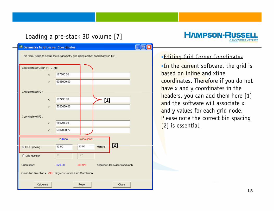
Editing Grid Corner CoordinatesIn the current software the grid isIn the current software, the grid is
based on inline and xline coordinates. Therefore if you do not have x and y coordinates in the headers, you can add them here [1] and the software will associate x and y values for each grid node. Please note the correct bin spacing
[1]
Please note the correct bin spacing [2] is essential.
[2][2]
10
Loading a post-stack 3D volume [8]g p [ ]
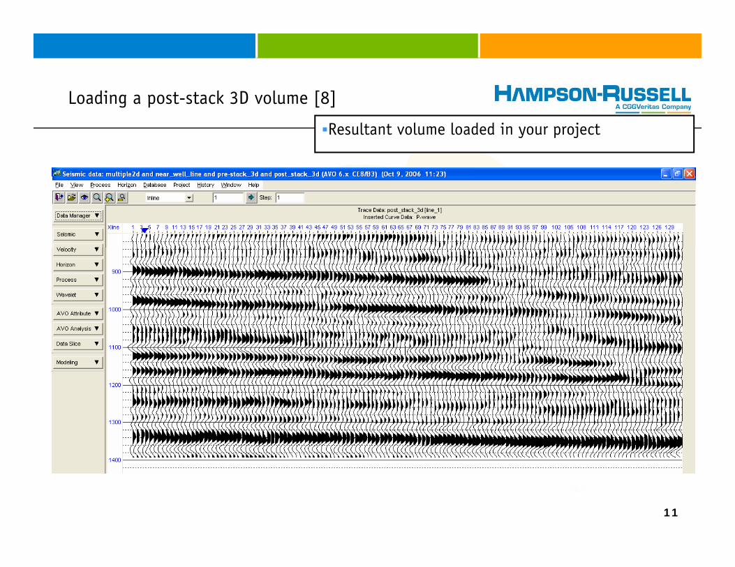
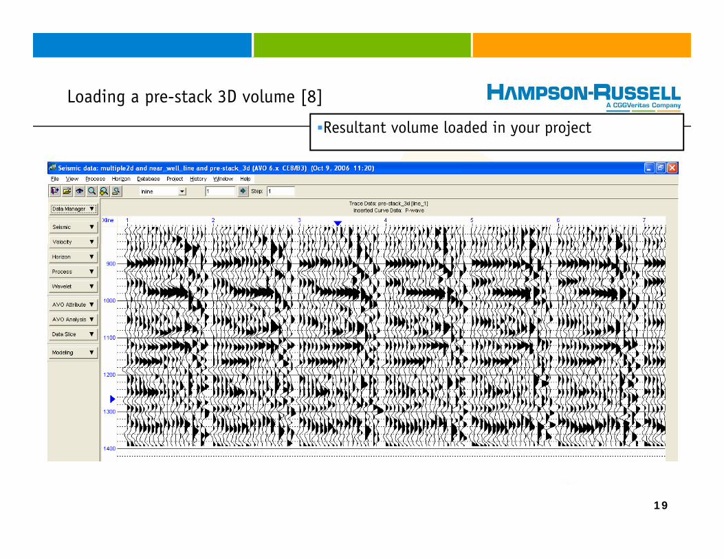
Resultant volume loaded in your project
11
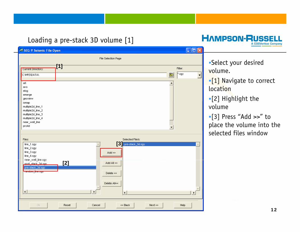
Loading a pre-stack 3D volume [1]g p [ ]
Select your desired volume.
[1]volume. [1] Navigate to correct
location[2] Highlight the [ ] g g
volume[3] Press “Add >>” to
place the volume into the l d fil i dselected files window
[3]
[2]
12
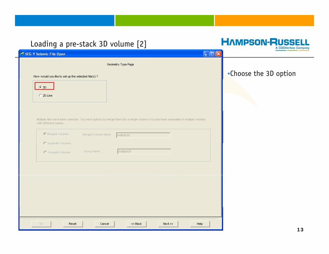
Loading a pre-stack 3D volume [2]g p [ ]
Choose the 3D option
13

Loading a pre-stack 3D volume [3]g p [ ]
Set the parameters for your segy volume:[1] In this example I have[4] [1] In this example I have
inline, xline, x and y coordinates in the headers. Therefore I toggle on “yes” for both. Use the Header Dump (highlighted in
[4]
orange) to find this information.[2] Assign the bin locations to
inline and xline[3] Say “yes” to renumber the
CDP ti ll[1]
CDPs sequentially[4] The name of segy file shown
in your project, by default, will be the same name as segy file.
[2]
[3]
14
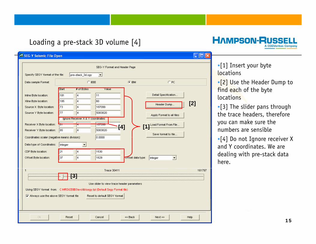
Loading a pre-stack 3D volume [4]g p [ ]
[1] Insert your byte locations[2] Use the Header Dump to
find each of the byte locations[3] The slider pans through[2] [3] The slider pans through
the trace headers, therefore you can make sure the numbers are sensible[4] D t I i X
[1][4]
[4] Do not Ignore receiver X and Y coordinates. We are dealing with pre-stack data here.
[3]
15
Loading a pre-stack 3D volume [5]g p [ ]
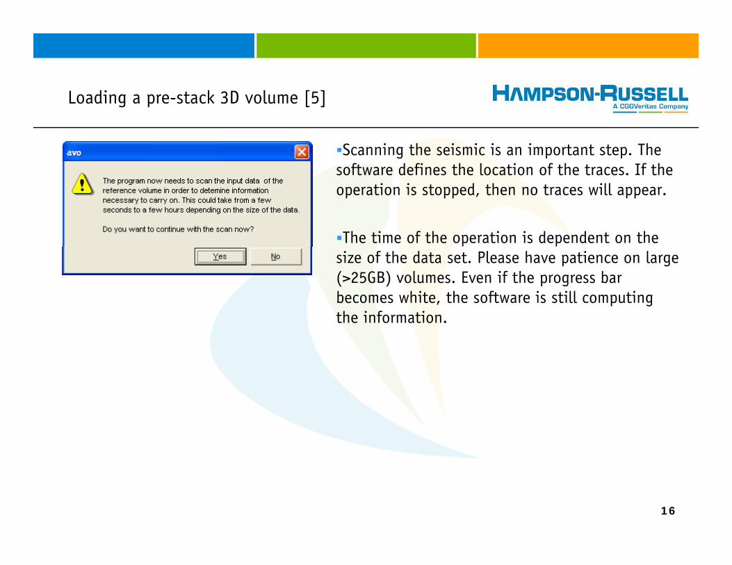
Scanning the seismic is an important step. The software defines the location of the traces. If the operation is stopped, then no traces will appear.
The time of the operation is dependent on the size of the data set. Please have patience on large (>25GB) volumes. Even if the progress bar becomes white, the software is still computing the informationthe information.
16
Loading a pre-stack 3D volume [6]g p [ ]
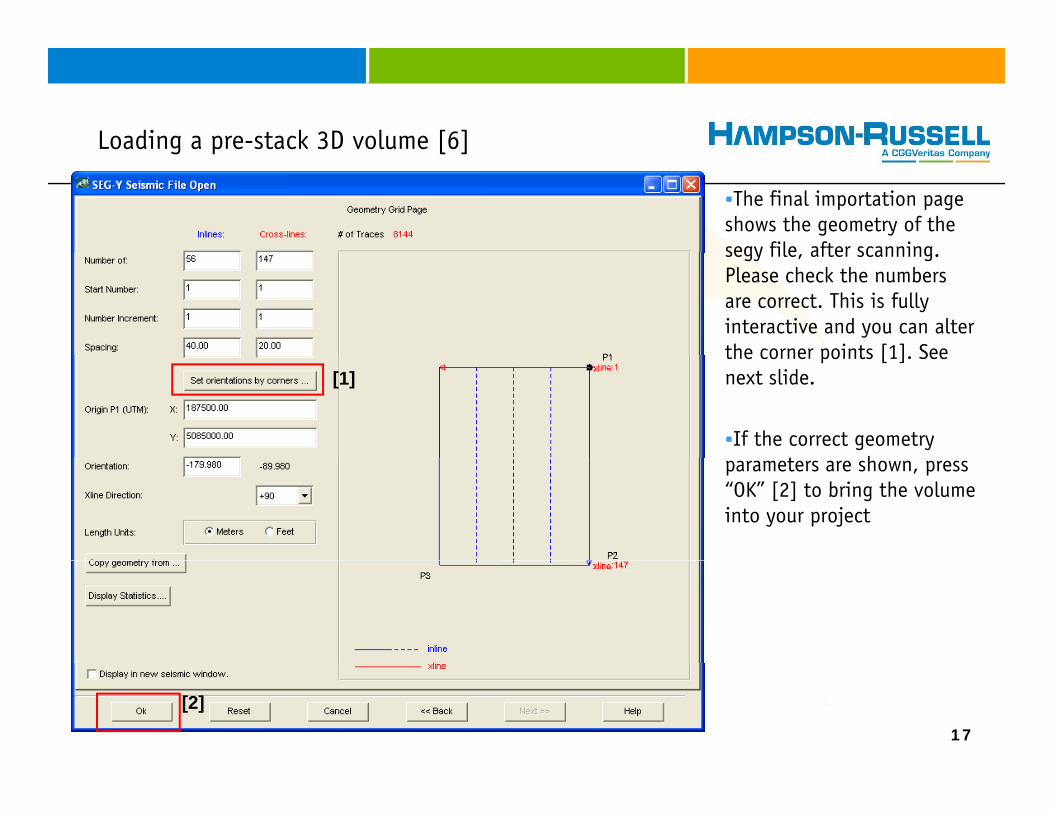
The final importation page shows the geometry of the segy file after scanningsegy file, after scanning. Please check the numbers are correct. This is fully interactive and you can alter the corner points [1] Seethe corner points [1]. See next slide.
If the correct geometry t h
[1]
parameters are shown, press “OK” [2] to bring the volume into your project
17
[2]
Loading a pre-stack 3D volume [7]g p [ ]
Editing Grid Corner CoordinatesIn the current software the grid isIn the current software, the grid is
based on inline and xline coordinates. Therefore if you do not have x and y coordinates in the headers, you can add them here [1] and the software will associate x and y values for each grid node. Please note the correct bin spacing
[1]
Please note the correct bin spacing [2] is essential.
[2][2]
18
Loading a pre-stack 3D volume [8]g p [ ]
Resultant volume loaded in your project
19
Loading a pre-stack 3D volume [9]g p [ ]
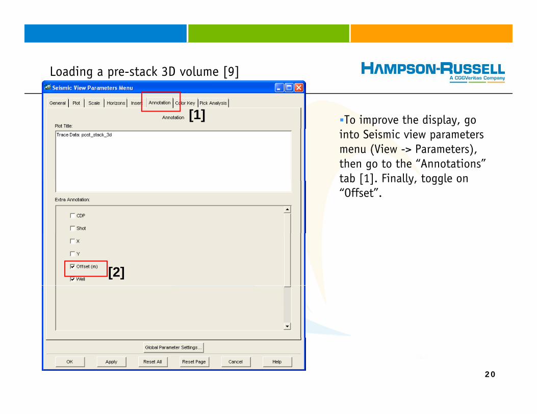
To improve the display, go [1]into Seismic view parameters menu (View -> Parameters), then go to the “Annotations” tab [1]. Finally, toggle ontab [1]. Finally, toggle on “Offset”.
[2]
20
Loading a pre-stack 3D volume [10]g p [ ]
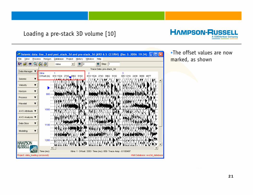
The offset values are now marked, as shownmarked, as shown
21
Loading a pre-stack 3D volume [11]g p [ ]
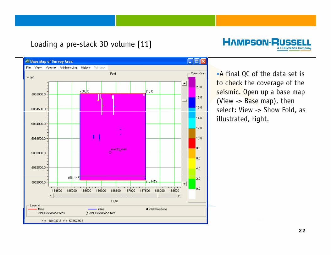
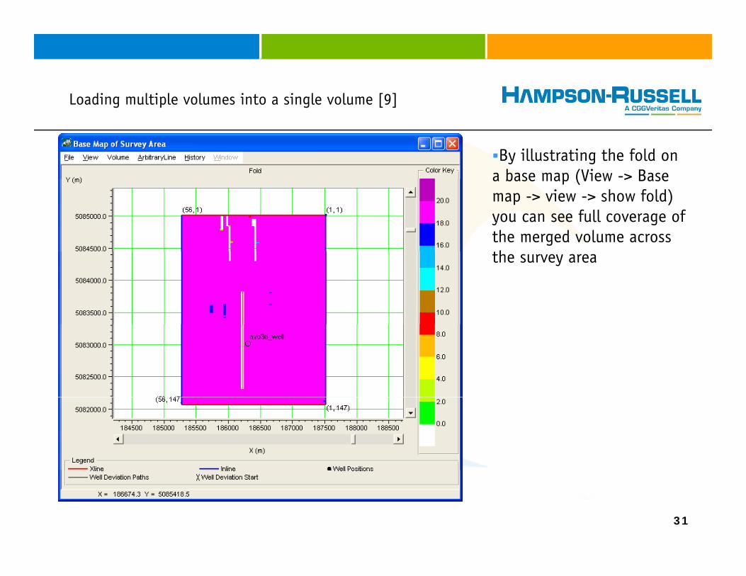
A final QC of the data set is to check the coverage of the seismic. Open up a base map (View -> Base map), then select: View -> Show Fold, asselect: View > Show Fold, as illustrated, right.
22
Loading multiple volumes into a single volume [1]
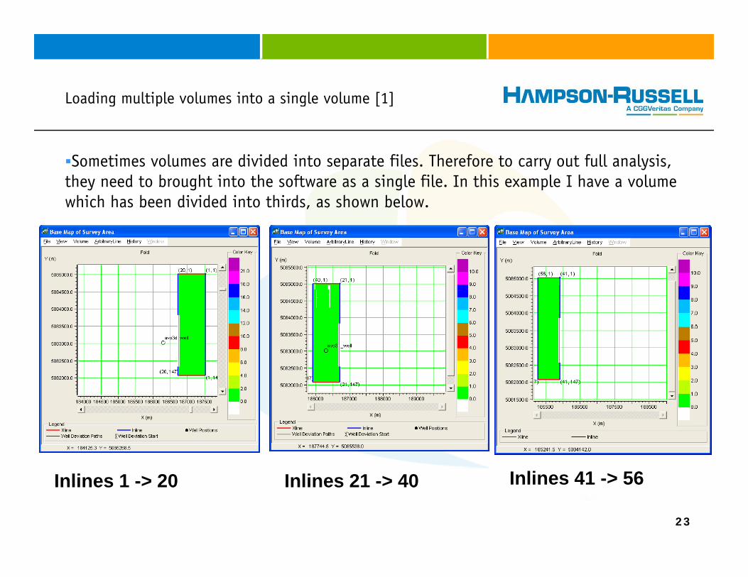
Sometimes volumes are divided into separate files. Therefore to carry out full analysis, they need to brought into the software as a single file In this example I have a volumethey need to brought into the software as a single file. In this example I have a volume which has been divided into thirds, as shown below.
23
Inlines 1 -> 20 Inlines 21 -> 40 Inlines 41 -> 56
Loading multiple volumes into a single volume [2]g p g [ ]
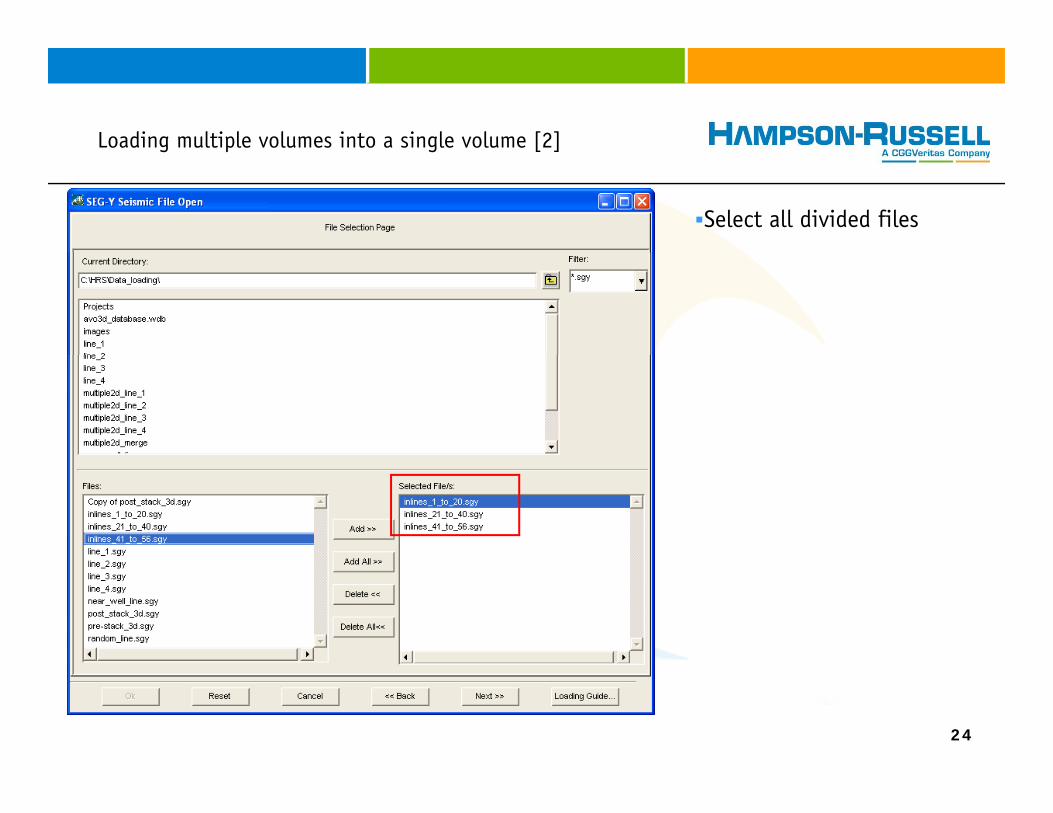
Select all divided files
24
Loading multiple volumes into a single volume [3]g p g [ ]
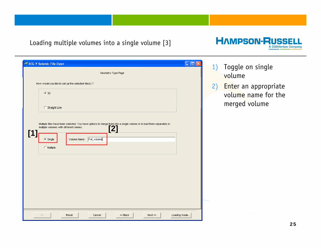
1) Toggle on single volumevolume
2) Enter an appropriate volume name for the merged volume
[1] [2]
25
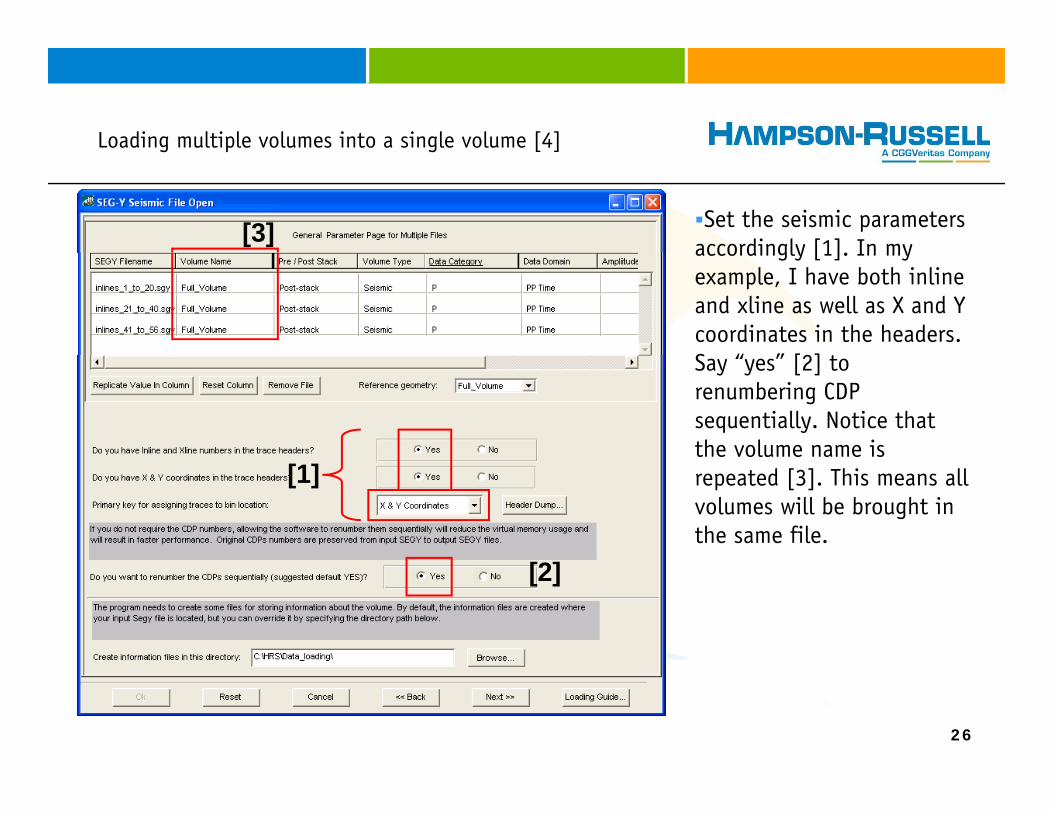
Loading multiple volumes into a single volume [4]g p g [ ]
Set the seismic parameters accordingly [1]. In my[3] accordingly [1]. In my example, I have both inline and xline as well as X and Y coordinates in the headers. S “ ” [2] tSay “yes” [2] to renumbering CDP sequentially. Notice that the volume name is repeated [3]. This means all volumes will be brought in the same file.
[1]
[2]
26
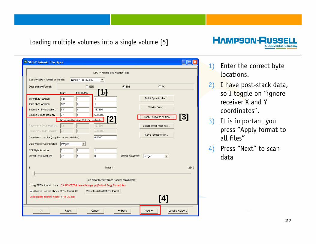
Loading multiple volumes into a single volume [5]g p g [ ]
1) Enter the correct byte locations.locations.
2) I have post-stack data, so I toggle on “ignore receiver X and Y
[1]
coordinates”.3) It is important you
press “Apply format to all files”
[2] [3]
all files4) Press “Next” to scan
data
[4]
27
[4]

Loading multiple volumes into a single volume [6]g p g [ ]
Scanning the seismic is an important step. The software defines the location of the traces. If the operation is stopped, then no traces will appear.
The time of the operation is dependent on the size of the data set. Please have patience on large (>25GB) volumes. Even if the progress bar becomes white, the software is still computing the information Do not resetthe information. Do not reset.
28
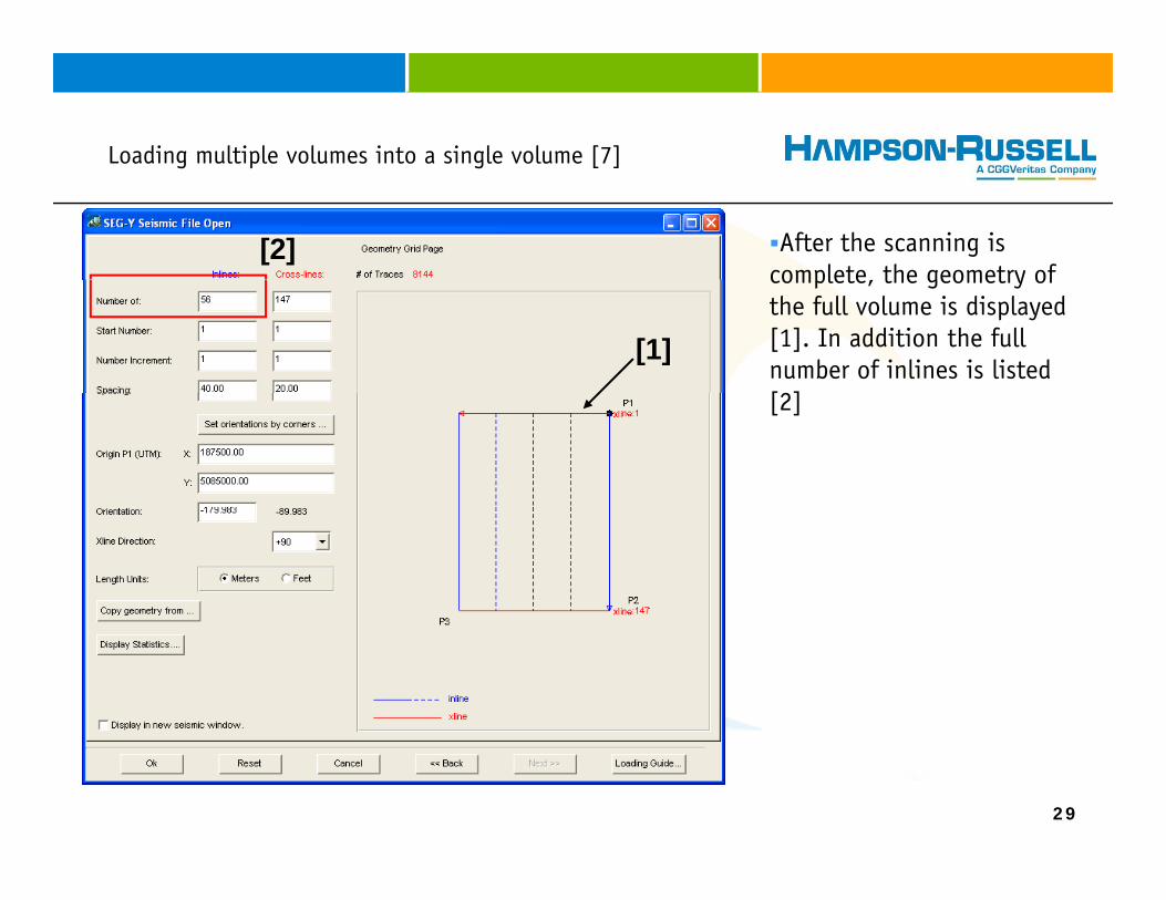
Loading multiple volumes into a single volume [7]g p g [ ]
After the scanning is complete, the geometry of
[2]complete, the geometry of the full volume is displayed [1]. In addition the full number of inlines is listed [2]
[1][2]
29
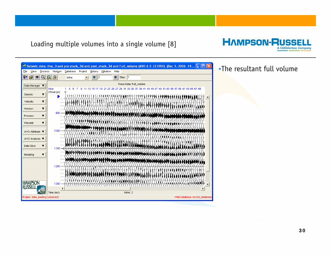
Loading multiple volumes into a single volume [8]g p g [ ]
The resultant full volume
30
Loading multiple volumes into a single volume [9]g p g [ ]
By illustrating the fold on a base map (View -> Basea base map (View > Base map -> view -> show fold) you can see full coverage of the merged volume across ththe survey area
31
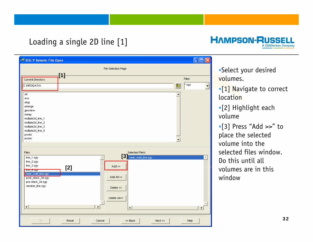
Loading a single 2D line [1]g g [ ]
Select your desired [1] volumes.
[1] Navigate to correct location[2] Hi hli ht h
[1]
[2] Highlight each volume[3] Press “Add >>” to
place the selectedplace the selected volume into the selected files window. Do this until all
l i hi[2]
[3]
volumes are in this window
[2]
32
Loading a single 2D line [2]g g [ ]
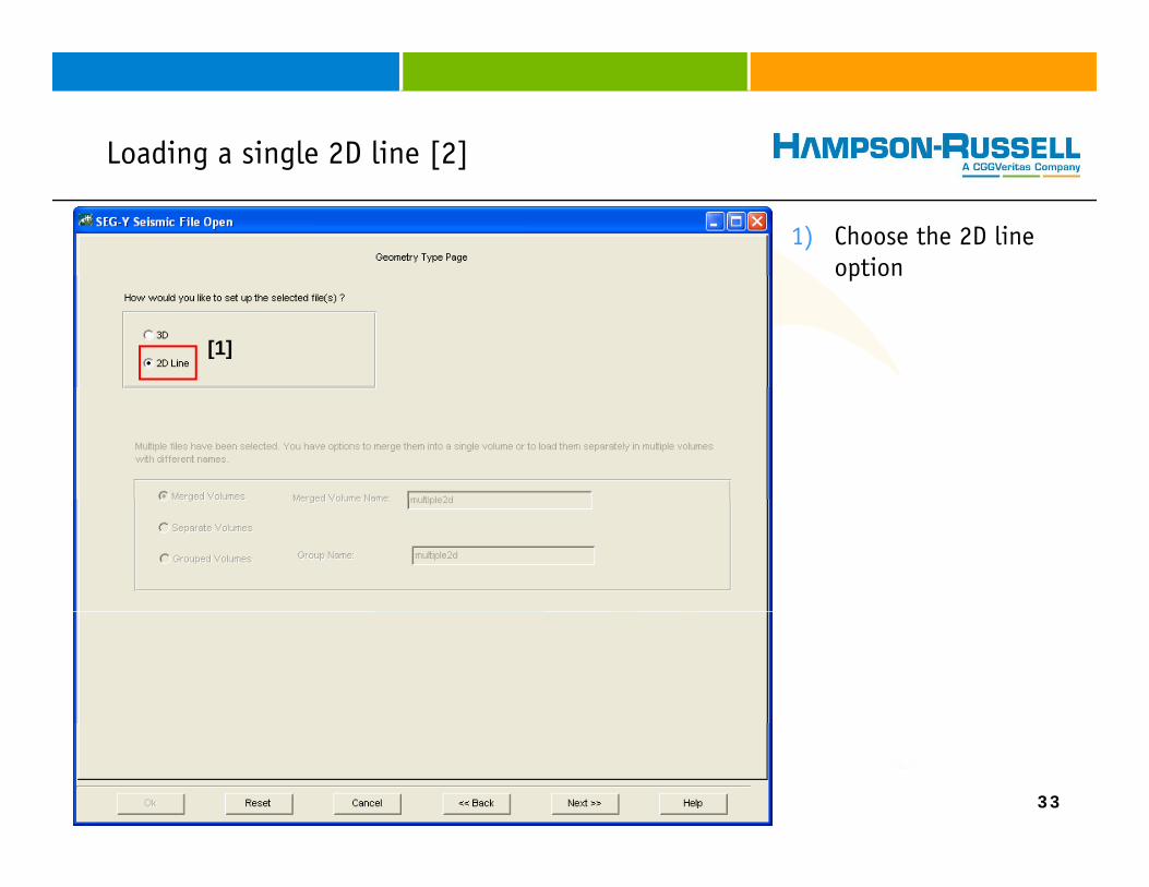
1) Choose the 2D line optionopt o
[1]
33
Loading a single 2D line [3]g g [ ]
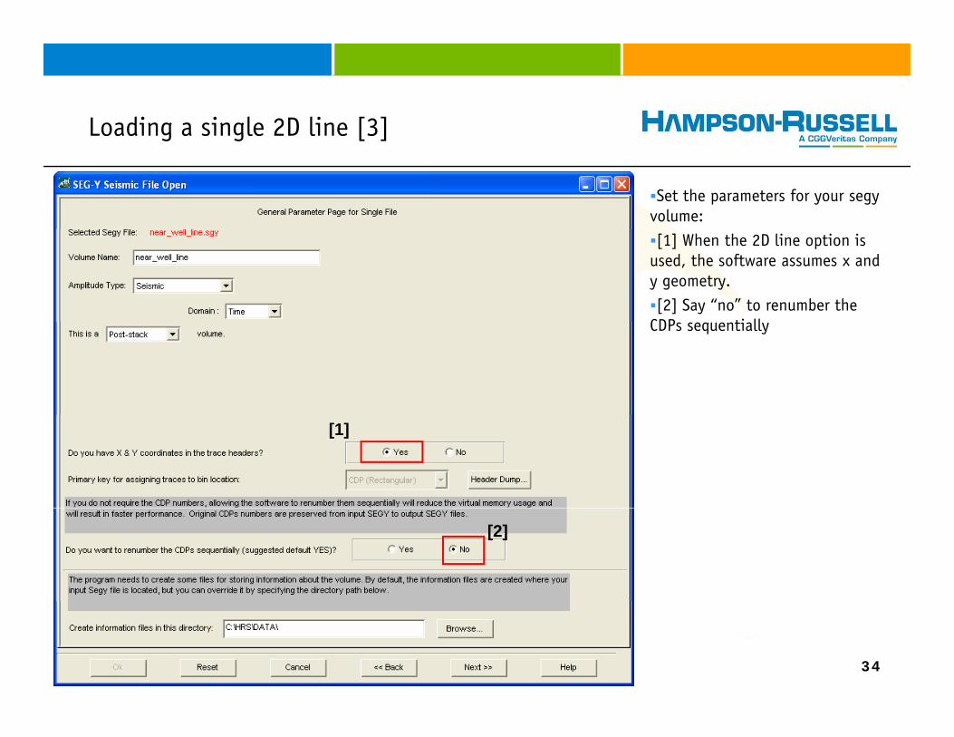
Set the parameters for your segy volume:[1] When the 2D line option is
used, the software assumes x and y geometry.[2] Say “no” to renumber the
CDP ti llCDPs sequentially
[1]
[2]
34
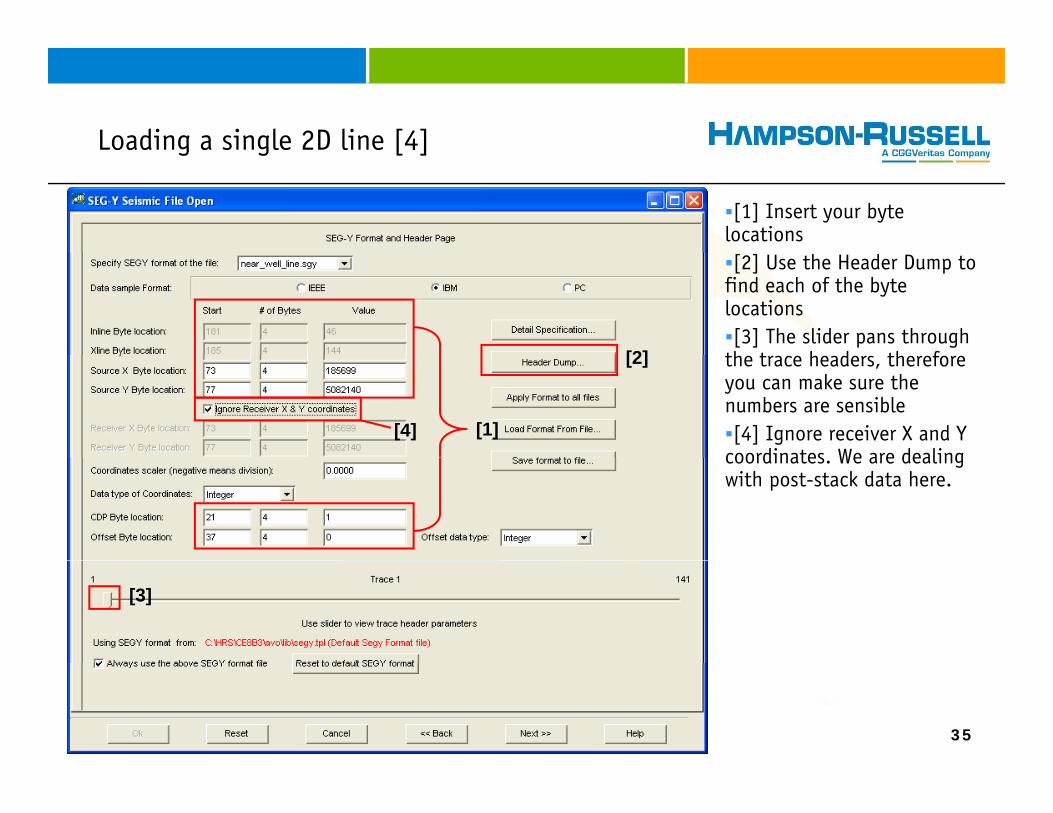
Loading a single 2D line [4]g g [ ]
[1] Insert your byte locations[2] Use the Header Dump to
find each of the byte locations[3] The slider pans through
th t h d th f[2] the trace headers, therefore you can make sure the numbers are sensible[4] Ignore receiver X and Y
coordinates We are dealing[1]
[2]
[4]coordinates. We are dealing with post-stack data here.
[3]
35
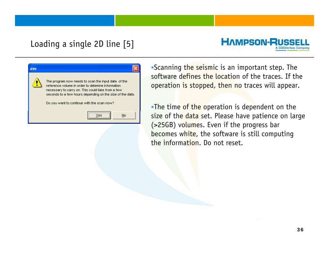
Loading a single 2D line [5]g g [ ]
Scanning the seismic is an important step. The software defines the location of the traces. If the operation is stopped, then no traces will appear.
The time of the operation is dependent on the size of the data set. Please have patience on large (>25GB) volumes. Even if the progress bar becomes white, the software is still computing the information Do not resetthe information. Do not reset.
36
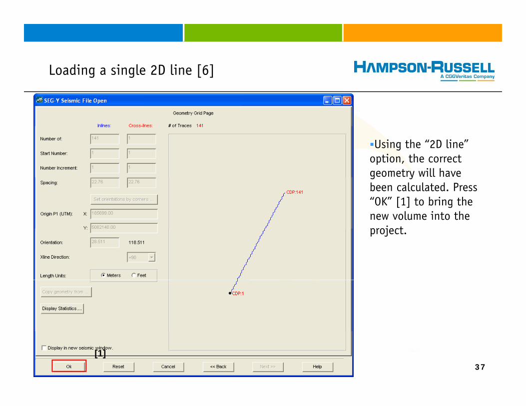
Loading a single 2D line [6]g g [ ]
Using the “2D line” option, the correct geometry will have g ybeen calculated. Press “OK” [1] to bring the new volume into the projectproject.
37
[1]

Loading a single 2D line [7]g g [ ]
Result of importation process, base-map displayed in bottom right
38
2D Line as a Single Line 3D Volume: Introductiong
It is usually inconvenient and time consuming to load in 2D data as a Straight Line. HRS software was designed for 3D volumes and consequently if you can load in a 2D line as a 3D volume, most workflows will be much easier for you. Most 2D SEG-Y files can easily be imported as a single line 3D it only requires that you can identify onecan easily be imported as a single line 3D – it only requires that you can identify one byte location in the Trace Header that is constant throughout the entire volume and use this to define the Inline.
This workflow will provide you with a quick way to successfully importing your 2D data as single-line 3D volume. It assumes that the file has X and Y coordinates
39
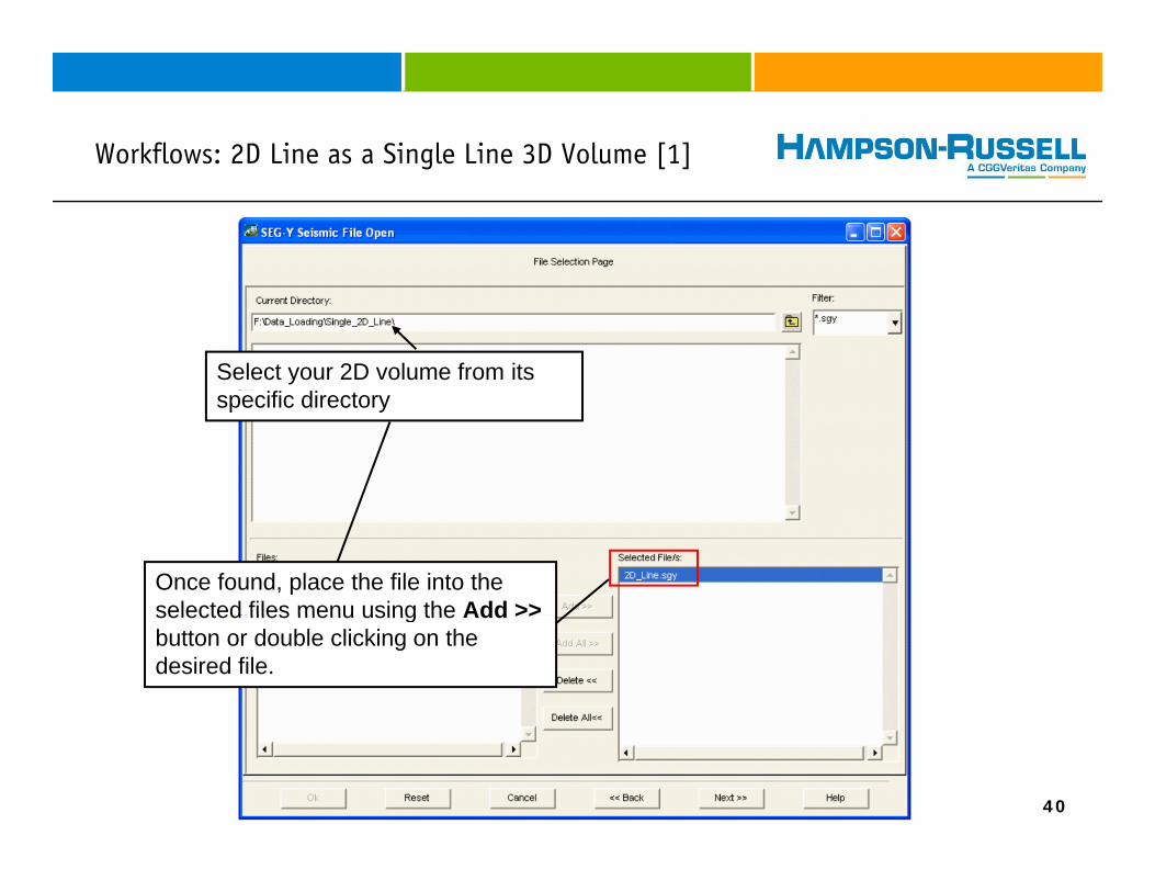
Workflows: 2D Line as a Single Line 3D Volume [1]g [ ]
Select your 2D volume from its specific directory
Once found, place the file into the selected files menu using the Add >>selected files menu using the Add >>button or double clicking on the desired file.
40
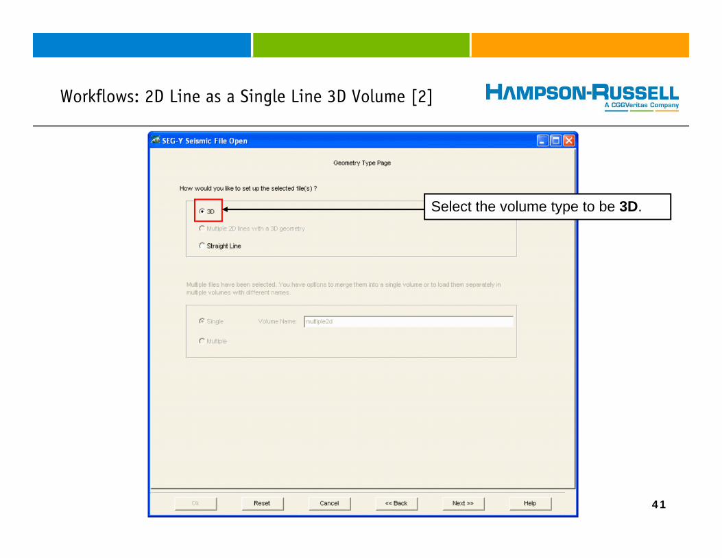
Workflows: 2D Line as a Single Line 3D Volume [2]g [ ]
Select the volume type to be 3D.
41
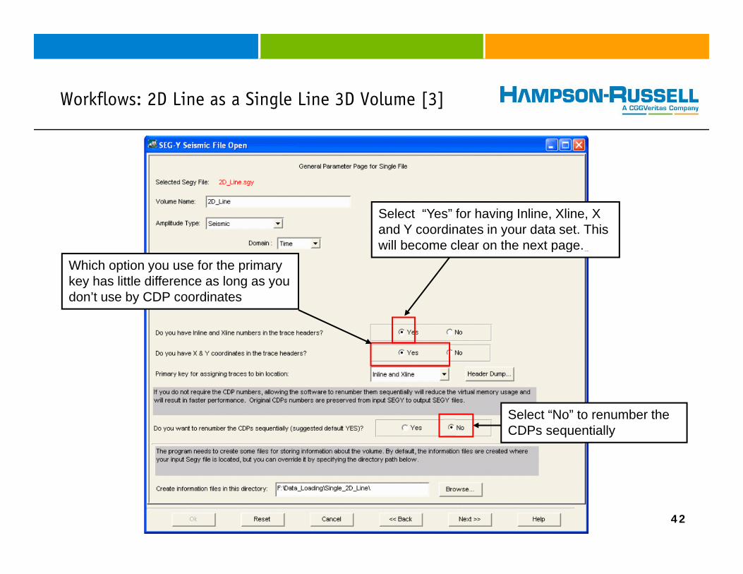
Workflows: 2D Line as a Single Line 3D Volume [3]g [ ]
Select “Yes” for having Inline, Xline, X and Y coordinates in your data set. This will become clear on the next page.p g
Which option you use for the primary key has little difference as long as you don’t use by CDP coordinates
Select “No” to renumber the CDPs sequentially
42
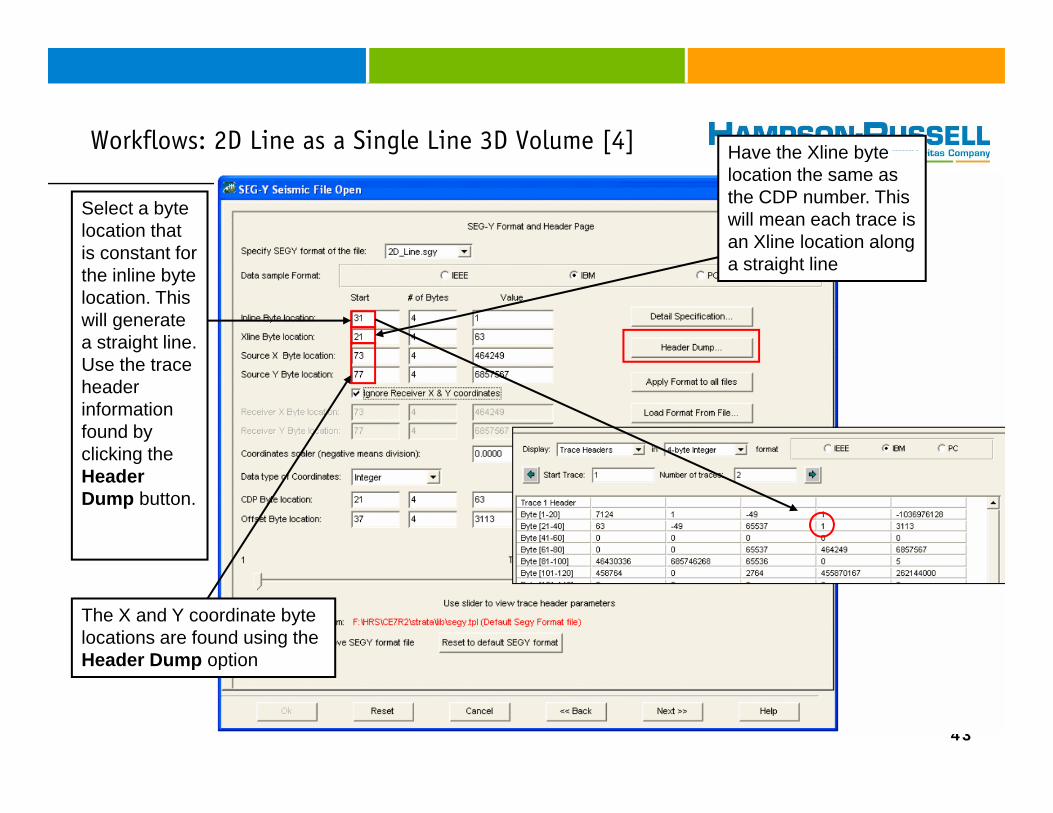
Workflows: 2D Line as a Single Line 3D Volume [4] Have the Xline byteg [ ]
Select a byte location that is constant for
Have the Xline byte location the same as the CDP number. This will mean each trace is an Xline location along is constant for
the inline byte location. This will generate a straight line.
a straight line
Use the trace header information found by clicking theclicking the Header Dump button.
The X and Y coordinate byte locations are found using the Header Dump option
43
Header Dump option
Workflows: 2D Line as a Single Line 3D Volume [5]g [ ]
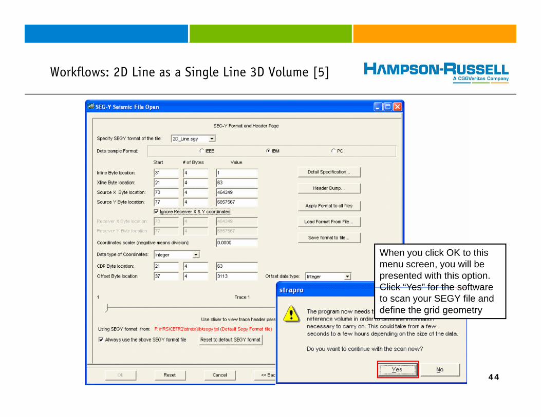
When you click OK to this menu screen, you will be presented with this option. Click “Yes” for the softwareClick Yes for the software to scan your SEGY file and define the grid geometry
44
Workflows: 2D Line as a Single Line 3D Volume [6]g [ ]
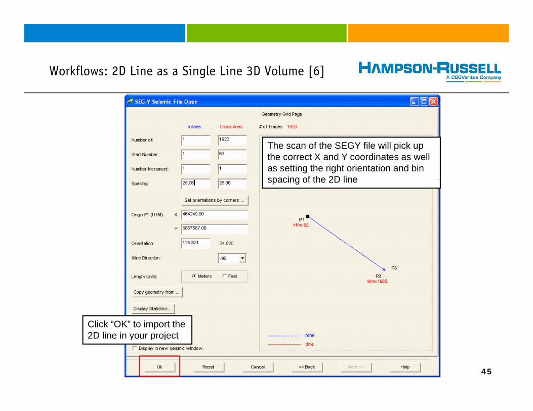
The scan of the SEGY file will pick up the correct X and Y coordinates as well as setting the right orientation and bin spacing of the 2D linespacing of the 2D line
Click “OK” to import the 2D line in your project
45
2D line in your project
Workflows: 2D Line as a Single Line 3D Volume [7]g [ ]
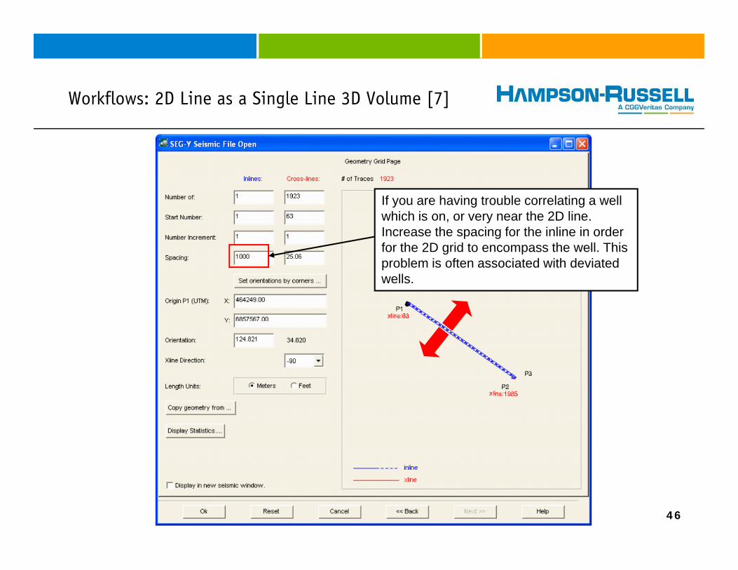
If you are having trouble correlating a well which is on, or very near the 2D line. Increase the spacing for the inline in order for the 2D grid to encompass the well Thisfor the 2D grid to encompass the well. This problem is often associated with deviated wells.
46
Loading a random 2D line [1]g [ ]
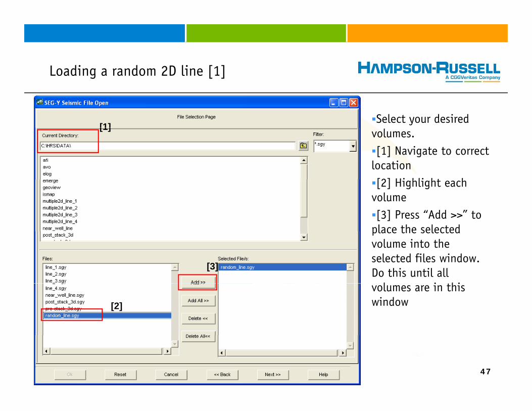
Select your desired [1]
volumes. [1] Navigate to correct
location[2] Hi hli ht h
[1]
[2] Highlight each volume[3] Press “Add >>” to
place the selectedplace the selected volume into the selected files window. Do this until all
l i hi
[3]
volumes are in this window[2]
47
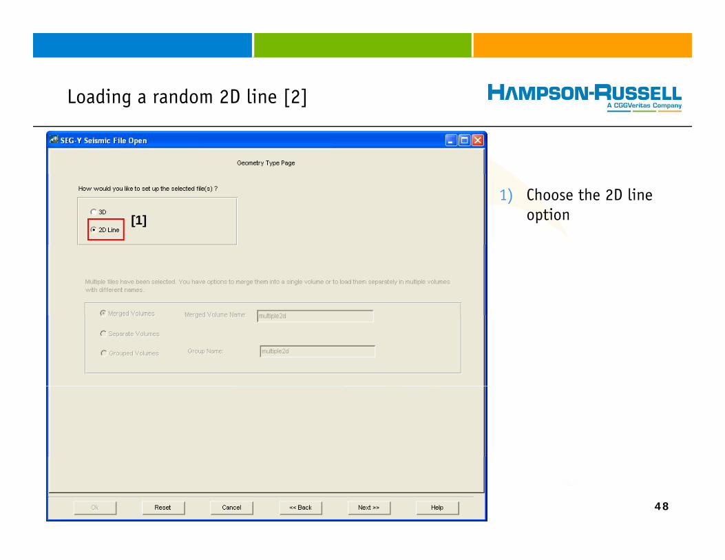
Loading a random 2D line [2]g [ ]
1) Choose the 2D line option[1]
48
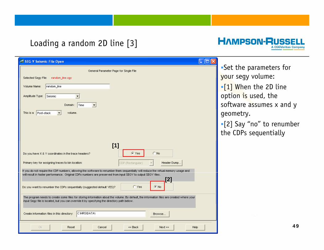
Loading a random 2D line [3]g [ ]
Set the parameters for your segy volume:your segy volume:[1] When the 2D line
option is used, the software assumes x and y geometry.[2] Say “no” to renumber
the CDPs sequentially
[1]
[2]
49

Loading a random 2D line [4]g [ ]
[1] Insert your byte locations[2] Use the Header Dump to
find each of the byte locations[3] The slider pans through
th t h d th f[2] the trace headers, therefore you can make sure the numbers are sensible[4] Ignore receiver X and Y
coordinates We are dealing[1]
[2]
[4]coordinates. We are dealing with post-stack data here.
[3]
50
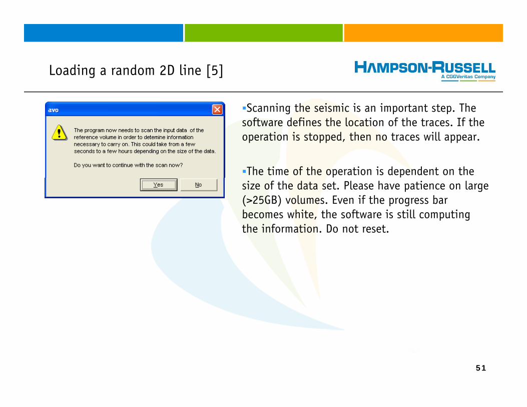
Loading a random 2D line [5]g [ ]
Scanning the seismic is an important step. The software defines the location of the traces. If the operation is stopped, then no traces will appear.
The time of the operation is dependent on the size of the data set. Please have patience on large (>25GB) volumes. Even if the progress bar becomes white, the software is still computing the information Do not resetthe information. Do not reset.
51
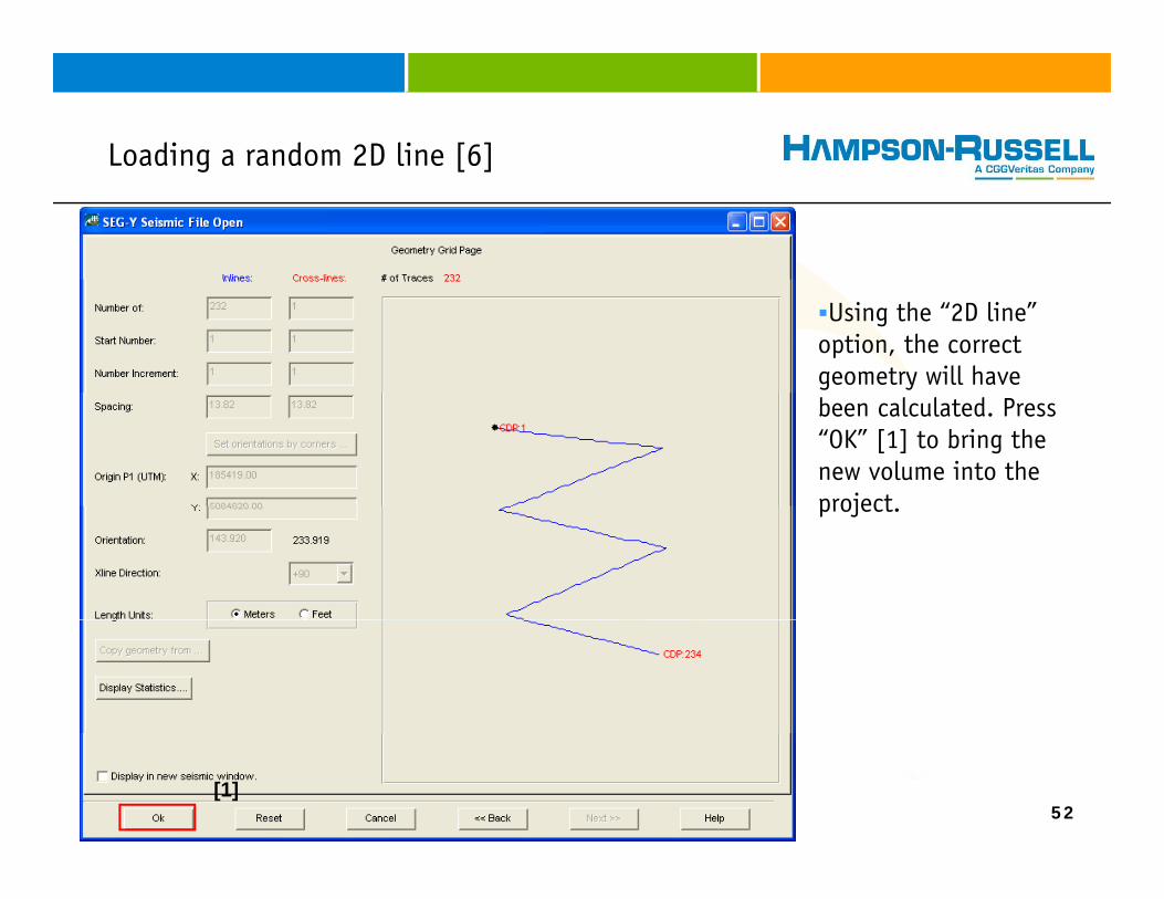
Loading a random 2D line [6]g [ ]
Using the “2D line” option, the correct geometry will have been calculated. Press “OK” [1] to bring the new volume into the projectproject.
52[1]
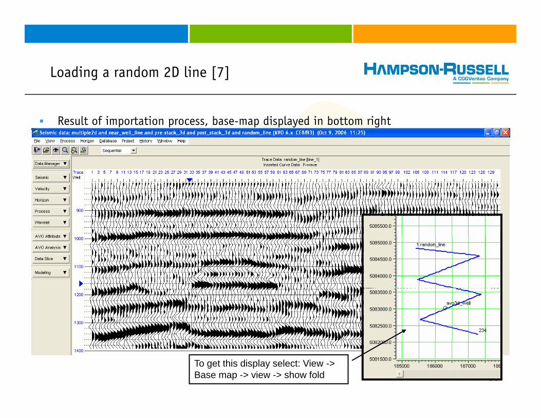
Loading a random 2D line [7]g [ ]
Result of importation process, base-map displayed in bottom right
53
To get this display select: View -> Base map -> view -> show fold
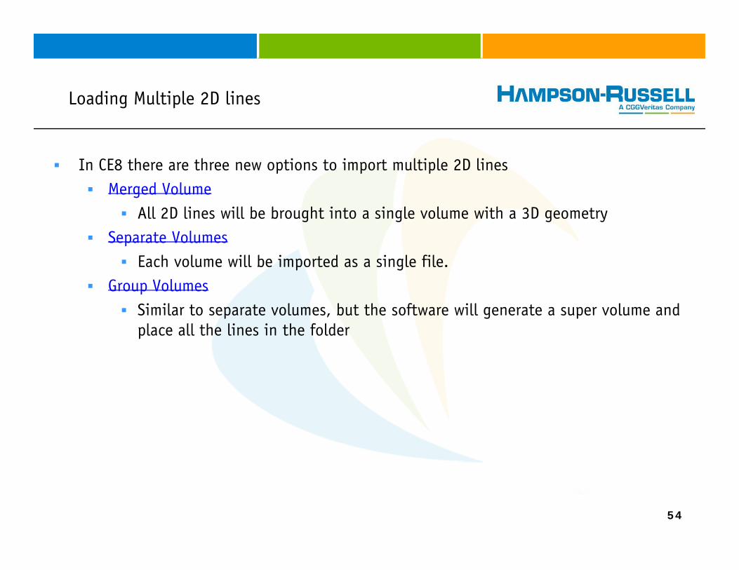
Loading Multiple 2D linesg p
In CE8 there are three new options to import multiple 2D linesMerged Volume
All 2D lines will be brought into a single volume with a 3D geometrySeparate Volumes
Each volume will be imported as a single file. Group Volumes
Similar to separate volumes, but the software will generate a super volume and place all the lines in the folder
54
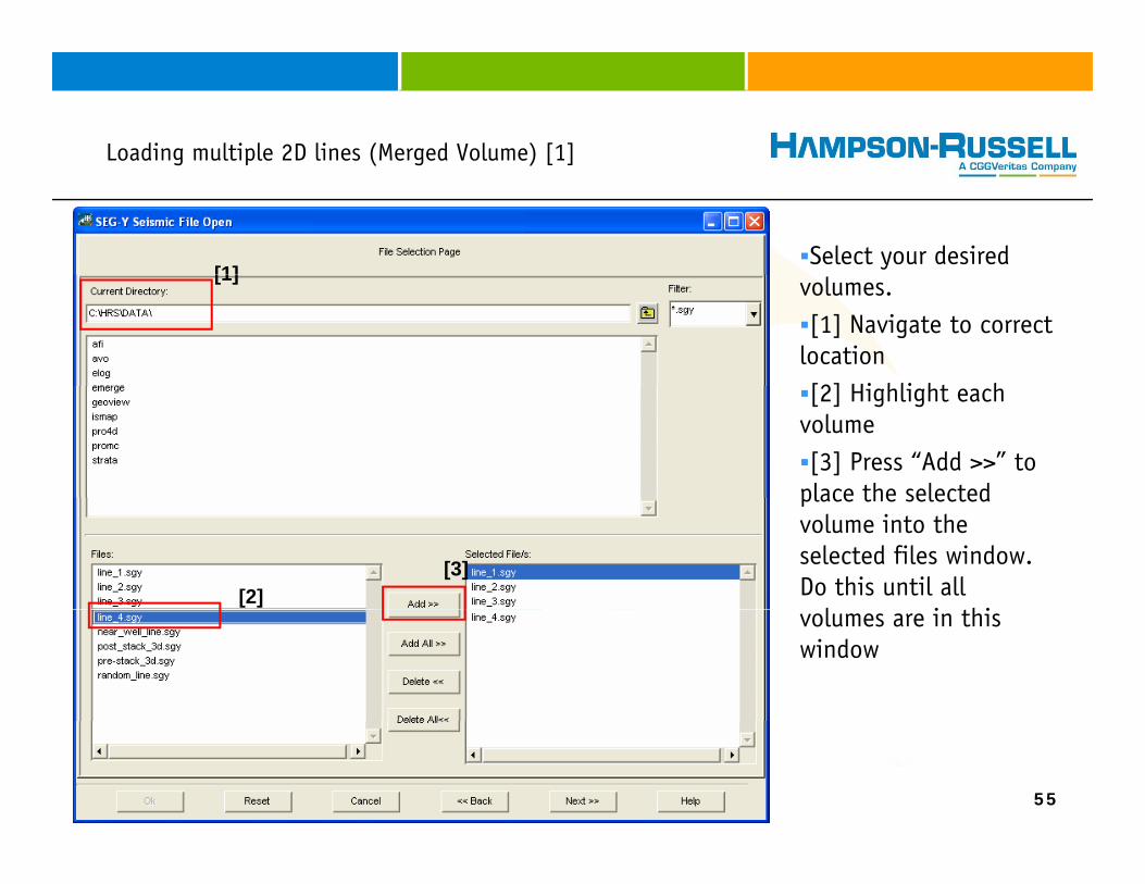
Loading multiple 2D lines (Merged Volume) [1]g p ( g ) [ ]
Select your desired [1] volumes.
[1] Navigate to correct location[2] Hi hli ht h
[1]
[2] Highlight each volume[3] Press “Add >>” to
place the selectedplace the selected volume into the selected files window. Do this until all
l i hi[2]
[3]
volumes are in this window
55
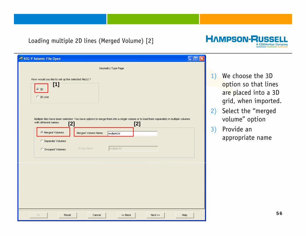
Loading multiple 2D lines (Merged Volume) [2]g p ( g ) [ ]
) W h h D1) We choose the 3D option so that lines are placed into a 3D grid, when imported.
[1]
g , p2) Select the “merged
volume” option3) Provide an
[2][2])
appropriate name
56
Loading multiple 2D lines (Merged Volume) [3]g p ( g ) [ ]
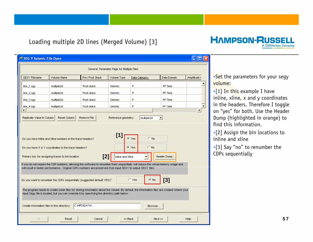
S t th t fSet the parameters for your segy volume:[1] In this example I have
inline, xline, x and y coordinates in the headers. Therefore I togglein the headers. Therefore I toggle on “yes” for both. Use the Header Dump (highlighted in orange) to find this information.[2] Assign the bin locations to [1]
inline and xline[3] Say “no” to renumber the
CDPs sequentially[2]
[1]
[3]
57
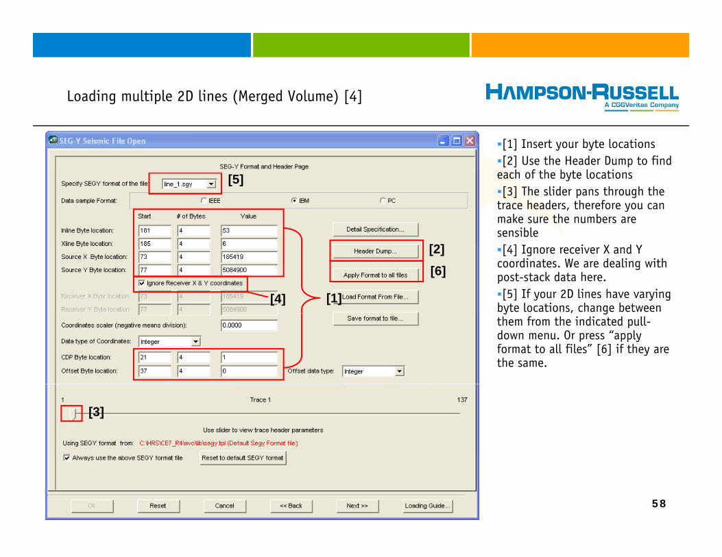
Loading multiple 2D lines (Merged Volume) [4]g p ( g ) [ ]
[1] Insert your byte locations[2] Use the Header Dump to find
each of the byte locationseach of the byte locations[3] The slider pans through the
trace headers, therefore you can make sure the numbers are sensible
[5]
[4] Ignore receiver X and Y coordinates. We are dealing with post-stack data here.[5] If your 2D lines have varying
byte locations, change between [1]
[2]
[4]
[6]
y gthem from the indicated pull-down menu. Or press “apply format to all files” [6] if they are the same.
[3]
58
Loading multiple 2D lines (Merged Volume) [5]g p ( g ) [ ]
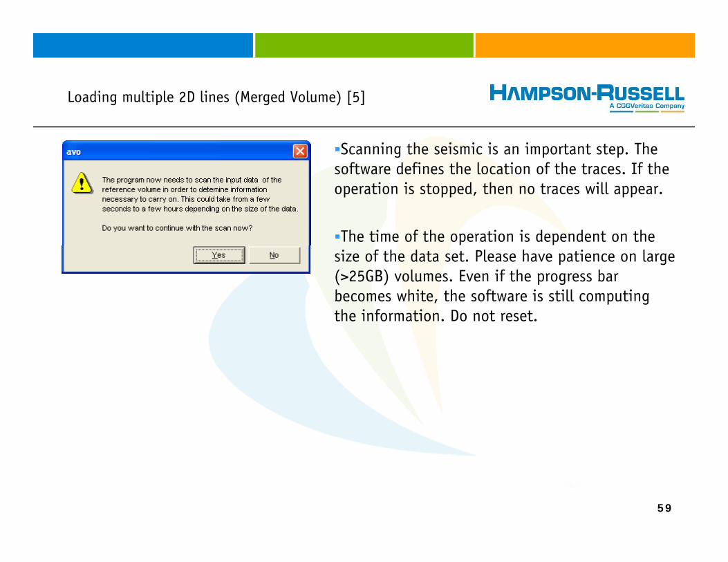
Scanning the seismic is an important step. The software defines the location of the traces. If the operation is stopped, then no traces will appear.
The time of the operation is dependent on the size of the data set. Please have patience on large (>25GB) volumes. Even if the progress bar becomes white, the software is still computing the information Do not resetthe information. Do not reset.
59
Loading multiple 2D lines (Merged Volume) [6]g p ( g ) [ ]
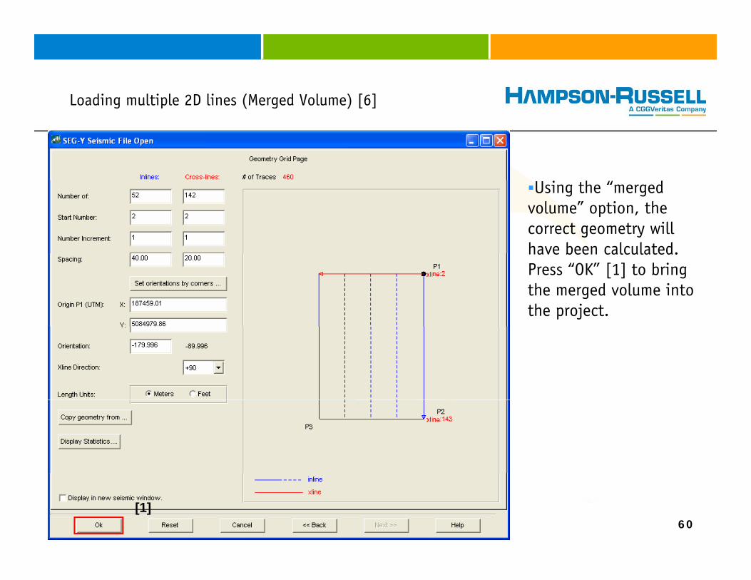
Using the “merged volume” option, the correct geometry will have been calculated.have been calculated. Press “OK” [1] to bring the merged volume into the project.
60[1]
Loading multiple 2D lines (Merged Volume) [7]g p ( g ) [ ]
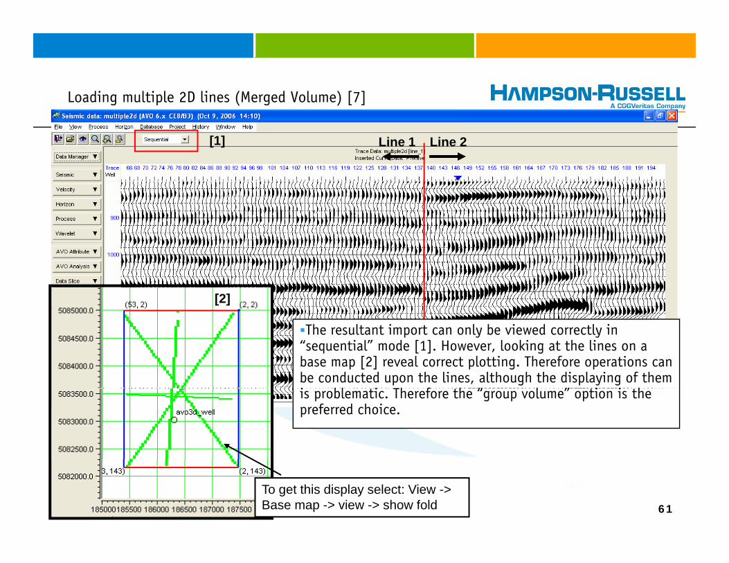
[1] Line 1 Line 2
[2]
The resultant import can only be viewed correctly in “sequential” mode [1]. However, looking at the lines on a base map [2] reveal correct plotting. Therefore operations can be conducted upon the lines, although the displaying of them i bl i Th f h “ l ” i i his problematic. Therefore the “group volume” option is the preferred choice.
61
To get this display select: View -> Base map -> view -> show fold

Loading multiple 2D lines (Separate Volume) [1]g p ( p ) [ ]
Select your desired [1] volumes.
[1] Navigate to correct location[2] Hi hli ht h
[1]
[2] Highlight each volume[3] Press “Add >>” to
place the selectedplace the selected volume into the selected files window. Do this until all
l i hi[2]
[3]
volumes are in this window
62
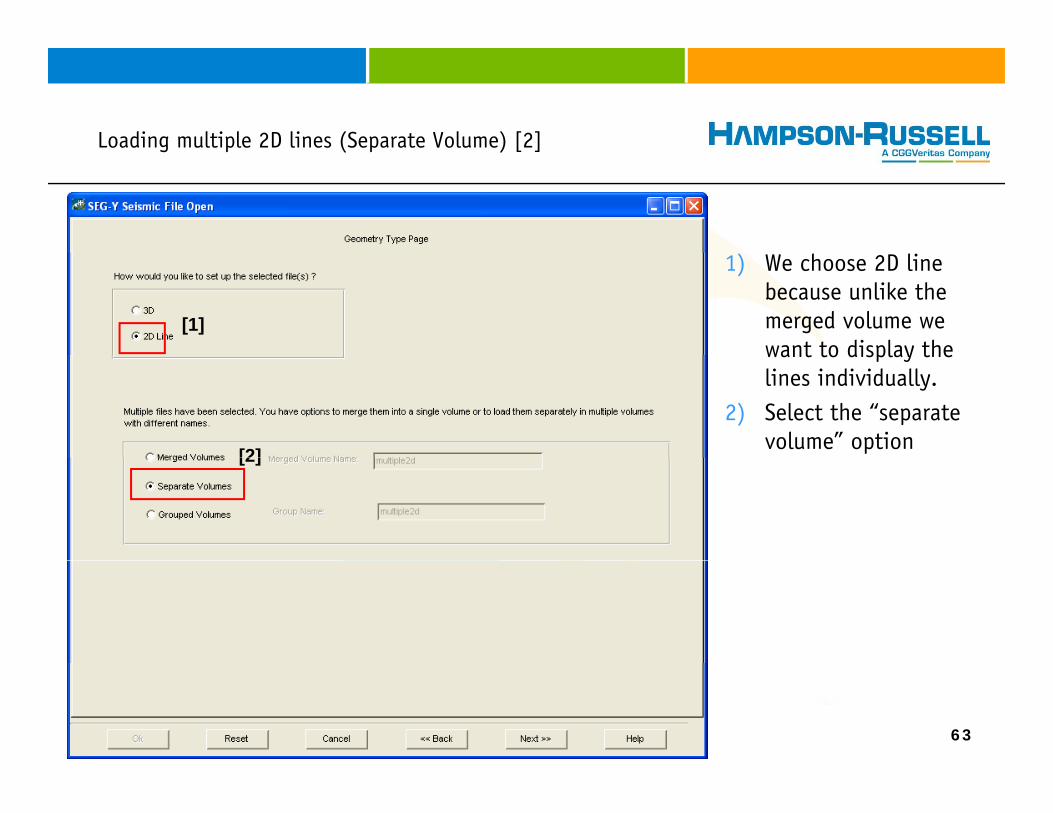
Loading multiple 2D lines (Separate Volume) [2]g p ( p ) [ ]
1) We choose 2D line because unlike the merged volume we want to display the
[1]want to display the lines individually.
2) Select the “separate volume” option
[2][2]
63
Loading multiple 2D lines (Separate Volume) [3]g p ( p ) [ ]
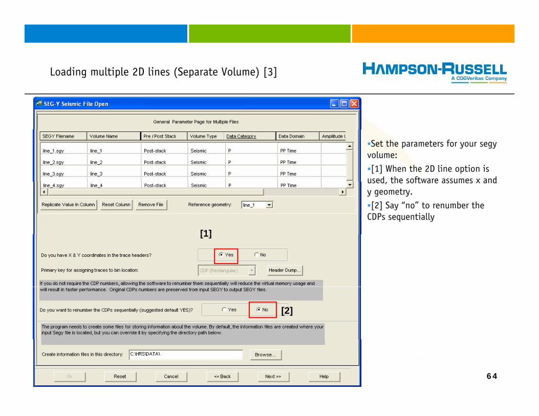
Set the parameters for your segy volume:[1] When the 2D line option is
used the software assumes x andused, the software assumes x and y geometry.[2] Say “no” to renumber the
CDPs sequentially
[1][1]
[2]
64
Loading multiple 2D lines (Separate Volume) [4]g p ( p ) [ ]
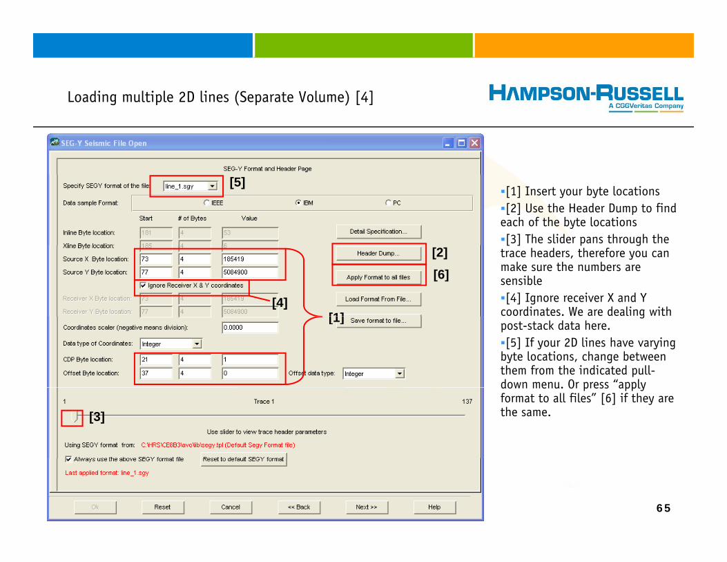
[1] Insert your byte locations[2] Use the Header Dump to find
each of the byte locations[3] The slider pans through the
[5]
[ ] p gtrace headers, therefore you can make sure the numbers are sensible[4] Ignore receiver X and Y
coordinates. We are dealing with [1]
[2]
[4]
[6]
gpost-stack data here.[5] If your 2D lines have varying
byte locations, change between them from the indicated pull-down menu. Or press “apply
[1]
down menu. Or press apply format to all files” [6] if they are the same.[3]
65

Loading multiple 2D lines (Separate Volume) [5]g p ( p ) [ ]
Scanning the seismic is an important step. The software defines the location of the traces. If the operation is stopped, then no traces will appear.
The time of the operation is dependent on the size of the data set. Please have patience on large (>25GB) volumes. Even if the progress bar becomes white, the software is still computing the information Do not resetthe information. Do not reset.
66

Loading multiple 2D lines (Separate Volume) [6]g p ( p ) [ ]
Using the “separate volume” option, the correct geometry will have been calculated.have been calculated. Press “OK” [1] to bring the merged volume into the project.
67
[1]

Loading multiple 2D lines (Separate Volume) [7]g p ( p ) [ ]
Image shows the 4 2D lines imported into the project
Base-map showing the 2D lines2D lines
68
To get this display select: View -> Base map -> view -> show fold
Loading multiple 2D lines (Separate Volume) [8]g p ( p ) [ ]
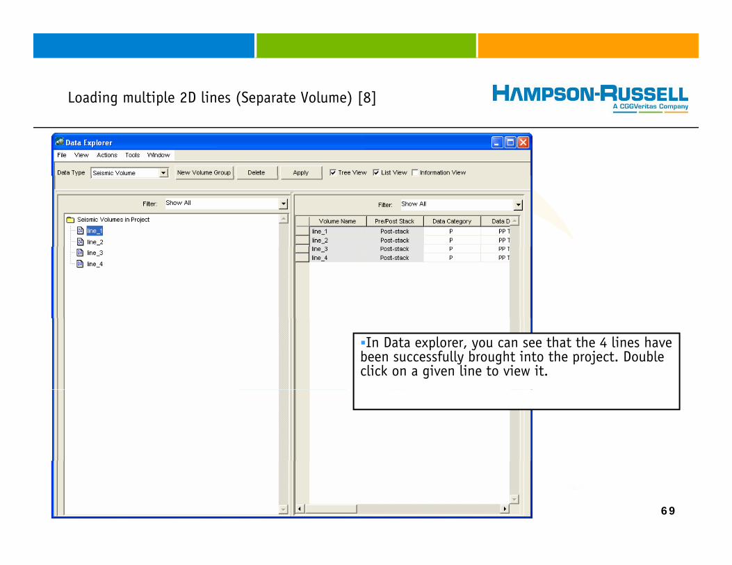
In Data explorer, you can see that the 4 lines have been successfully brought into the project. Double click on a given line to view it.
69
Loading multiple 2D lines (Grouped Volume) [1]g p ( p ) [ ]
l d d[1]
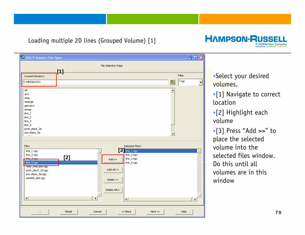
Select your desired volumes. [1] Navigate to correct
location
[1]
location[2] Highlight each
volume[3] Press “Add >>” to[3] Press Add >> to
place the selected volume into the selected files window. D thi til ll
[2][3]
Do this until all volumes are in this window
70
Loading multiple 2D lines (Grouped Volume) [2]g p ( p ) [ ]
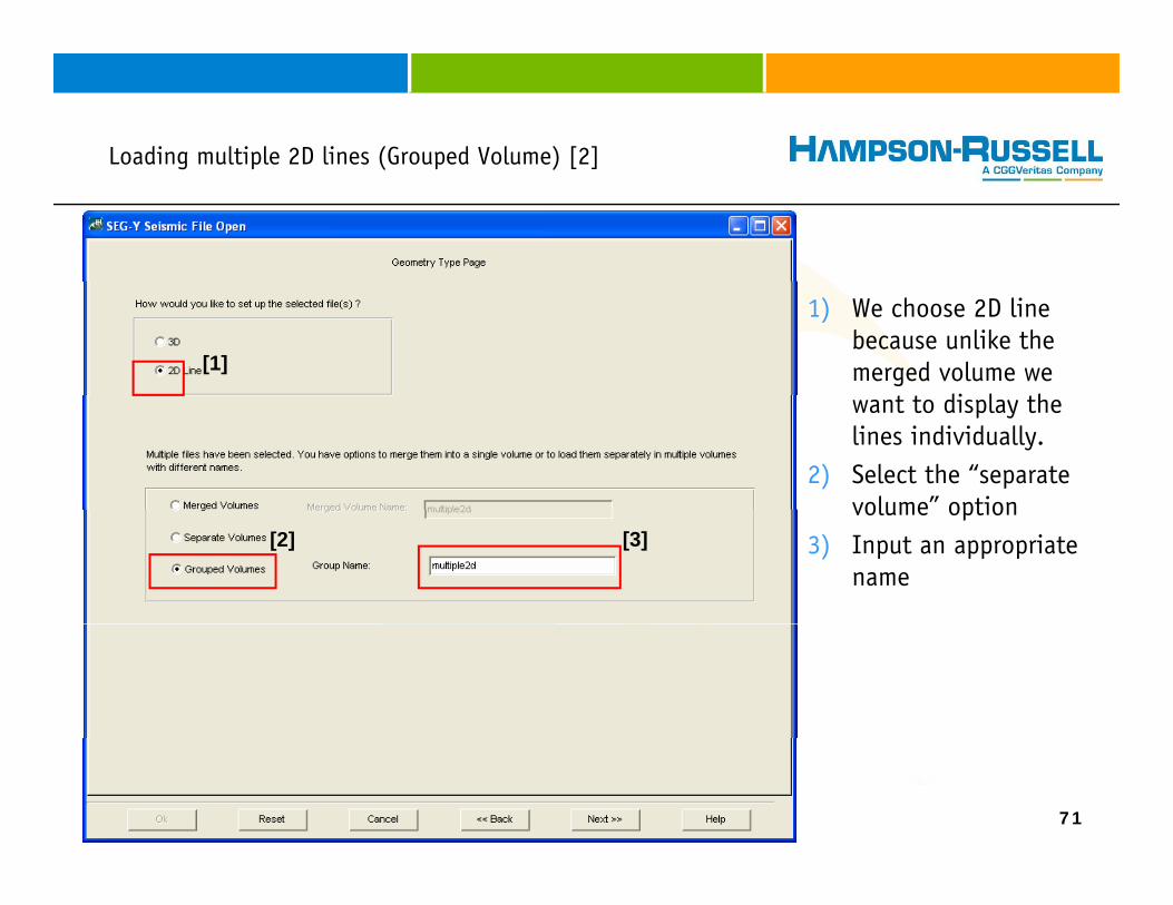
1) We choose 2D line because unlike the merged volume we
t t di l th
[1]
want to display the lines individually.
2) Select the “separate volume” optionvolume option
3) Input an appropriate name
[2] [3]
71
Loading multiple 2D lines (Grouped Volume) [3]g p ( p ) [ ]
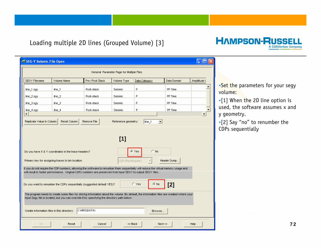
Set the parameters for your segy volume:[1] When the 2D line option is
used, the software assumes x andused, the software assumes x and y geometry.[2] Say “no” to renumber the
CDPs sequentially
[1][1]
[2]
72
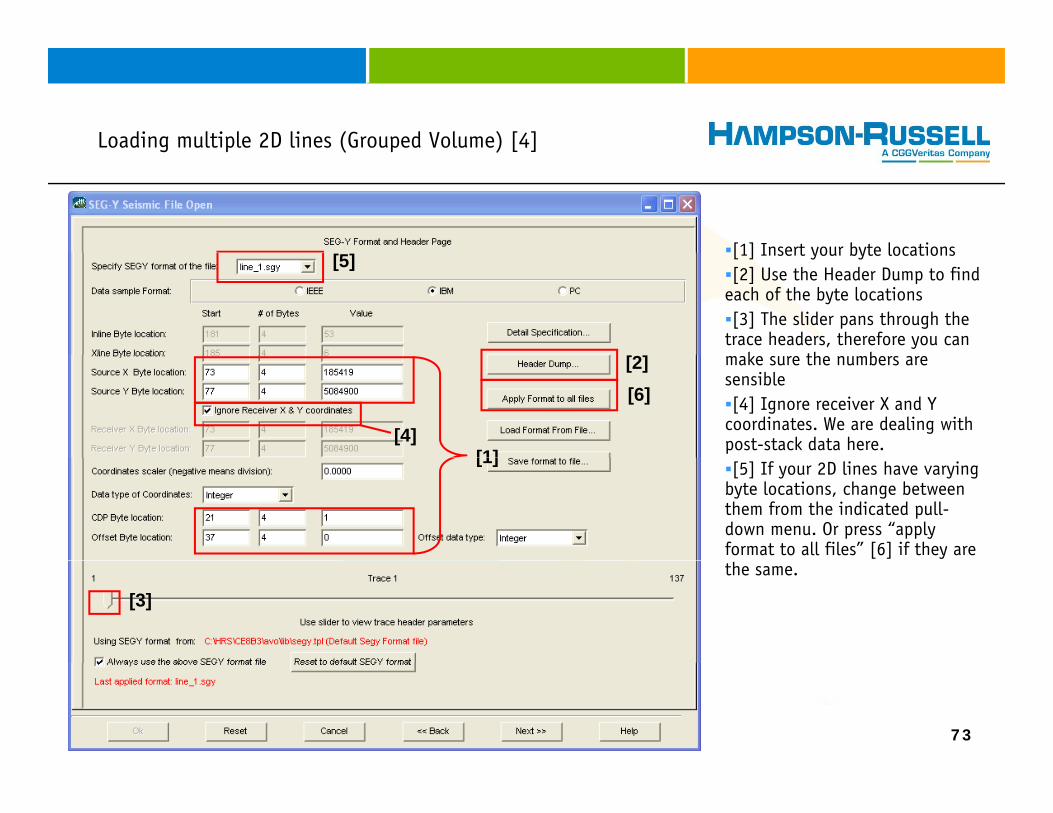
Loading multiple 2D lines (Grouped Volume) [4]g p ( p ) [ ]
[1] Insert your byte locations[1] Insert your byte locations[2] Use the Header Dump to find
each of the byte locations[3] The slider pans through the
trace headers, therefore you can k th b2
[5]
make sure the numbers are sensible[4] Ignore receiver X and Y
coordinates. We are dealing with post-stack data here.
[1]
[2]
[4]
[6]
[5] If your 2D lines have varying byte locations, change between them from the indicated pull-down menu. Or press “apply format to all files” [6] if they are
[1]
the same.
[3]
73

Loading multiple 2D lines (Grouped Volume) [5]g p ( p ) [ ]
Scanning the seismic is an important step. The software defines the location of the traces. If the operation is stopped, then no traces will appear.
The time of the operation is dependent on the size of the data set. Please have patience on large (>25GB) volumes. Even if the progress bar becomes white, the software is still computing the information Do not resetthe information. Do not reset.
74
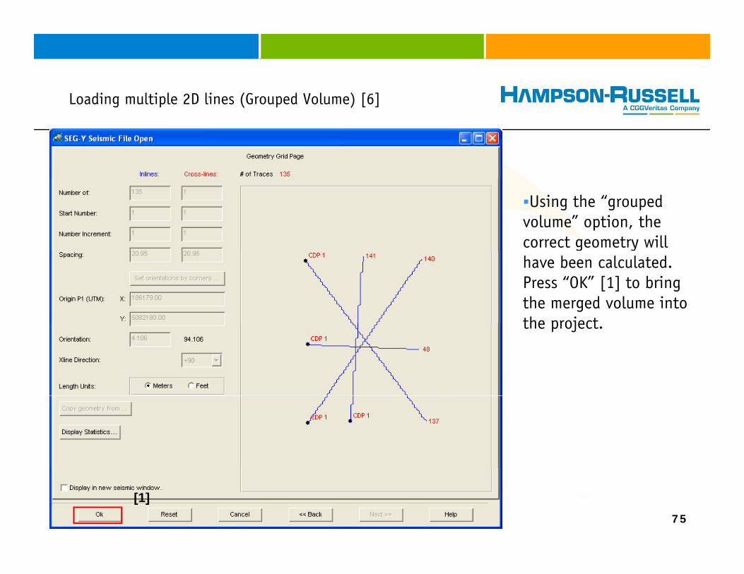
Loading multiple 2D lines (Grouped Volume) [6]g p ( p ) [ ]
Using the “grouped volume” option, the correct geometry will have been calculated. Press “OK” [1] to bring the merged volume into the projectthe project.
75
[1]
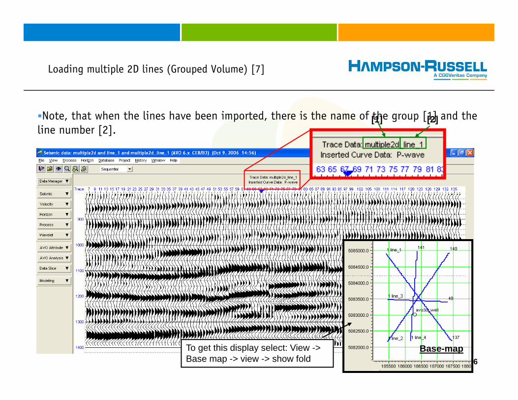
Loading multiple 2D lines (Grouped Volume) [7]g p ( p ) [ ]
Note, that when the lines have been imported, there is the name of the group [1] and the [1] [2]line number [2].
76
Base-mapTo get this display select: View -> Base map -> view -> show fold
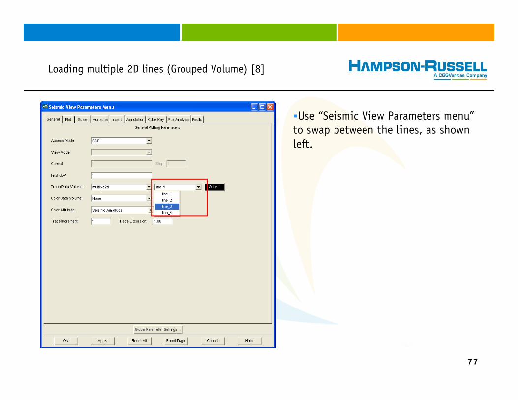
Loading multiple 2D lines (Grouped Volume) [8]g p ( p ) [ ]
Use “Seismic View Parameters menu” to swap between the lines, as shown left.
77
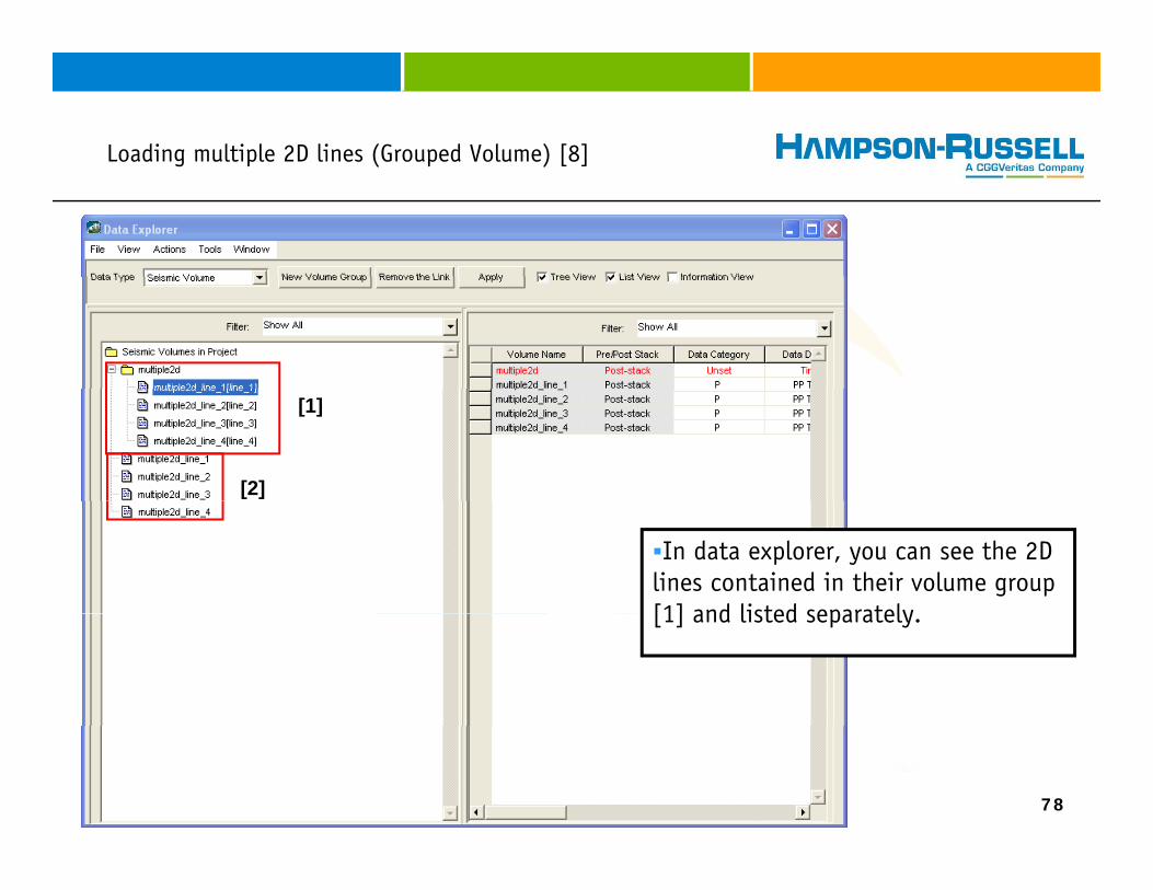
Loading multiple 2D lines (Grouped Volume) [8]g p ( p ) [ ]
[1]
[2]
In data explorer, you can see the 2D lines contained in their volume group [1] and listed separately[1] and listed separately.
78
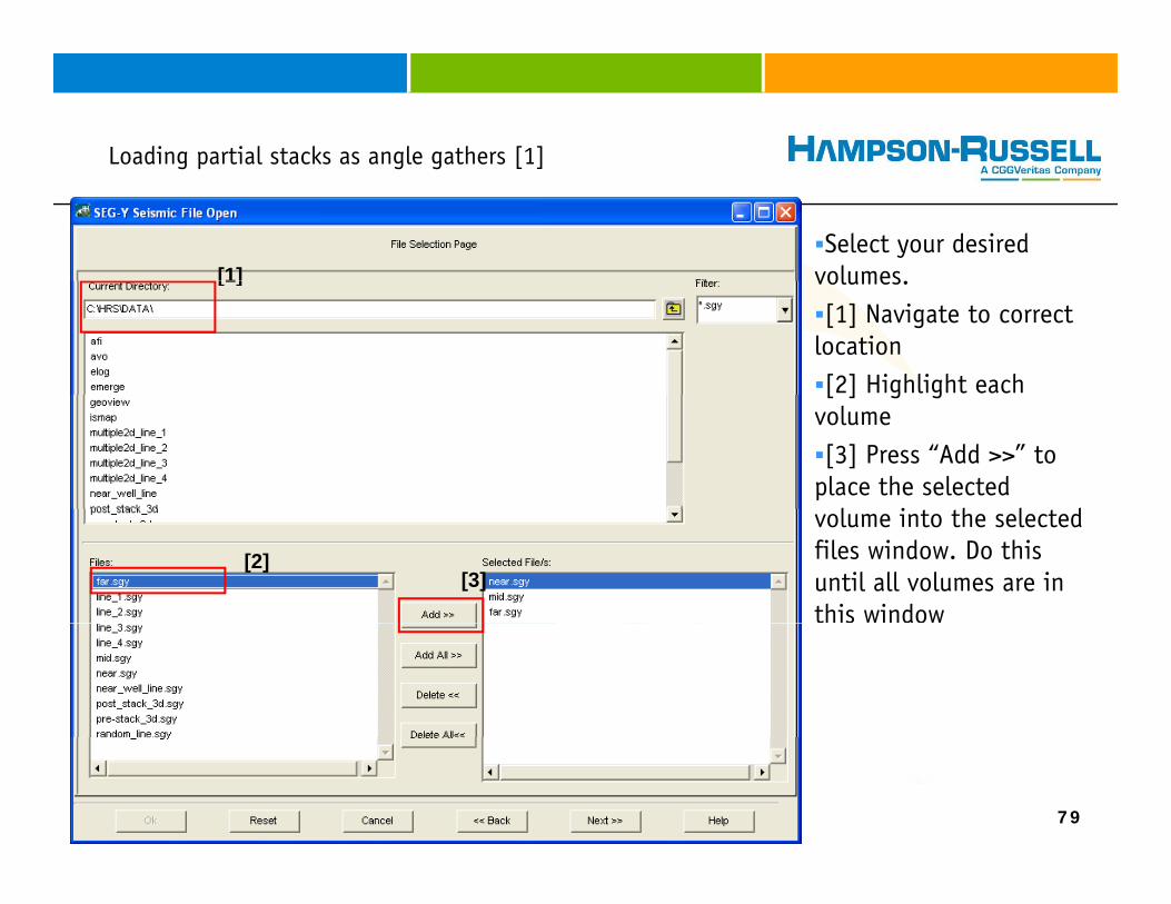
Loading partial stacks as angle gathers [1]g p g g [ ]
Select your desired volumes.
[1][1] volumes.
[1] Navigate to correct location[2] Highlight each
[1]
[ ] g gvolume[3] Press “Add >>” to
place the selected l i h l dvolume into the selected
files window. Do this until all volumes are in this window
[2] [3][2][3]
79
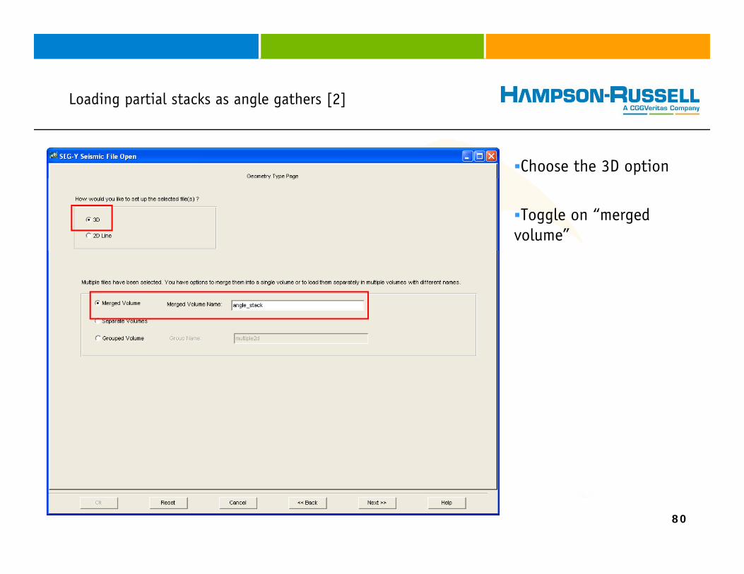
Loading partial stacks as angle gathers [2]g p g g [ ]
Choose the 3D option
Toggle on “merged volume”
80
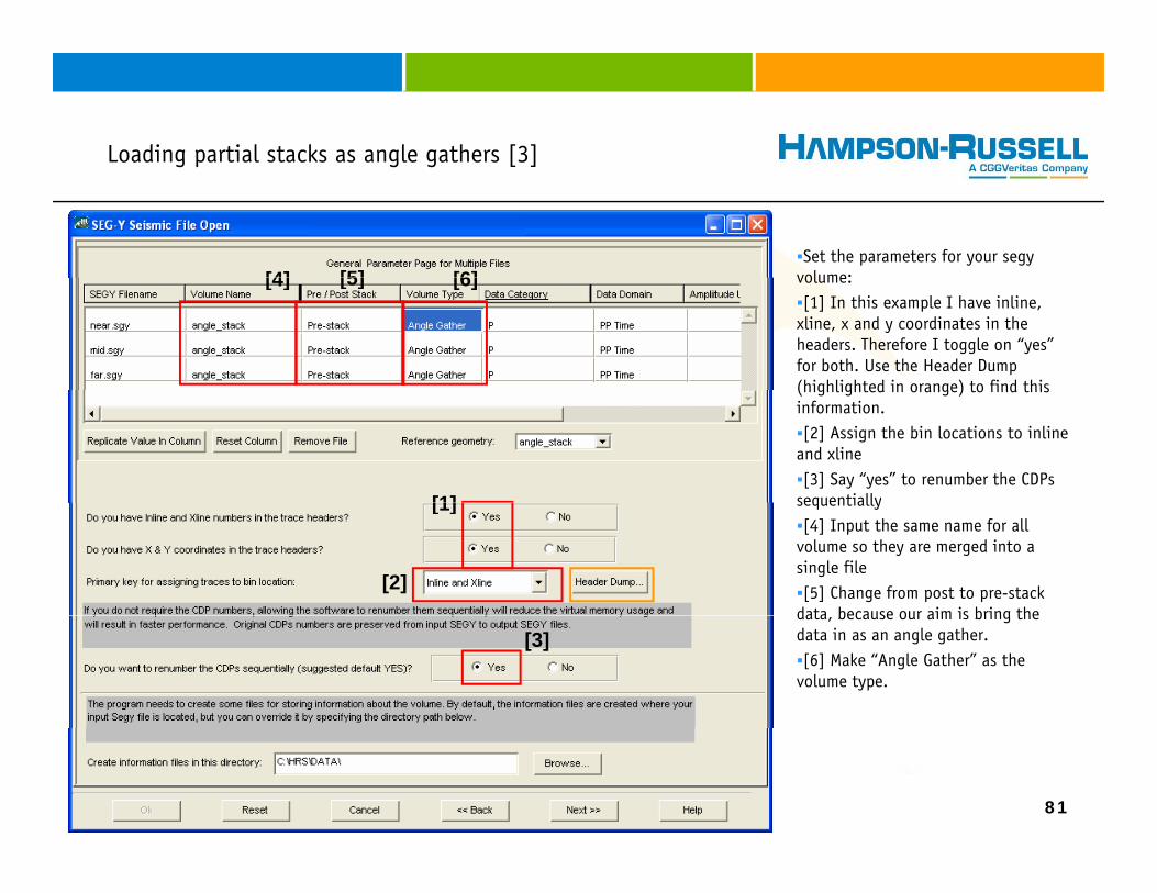
Loading partial stacks as angle gathers [3]g p g g [ ]
Set the parameters for your segy volume:[5] [6][4] volume:[1] In this example I have inline,
xline, x and y coordinates in the headers. Therefore I toggle on “yes” for both. Use the Header Dump (highlighted in orange) to find this
[5] [6][4]
(highlighted in orange) to find this information.[2] Assign the bin locations to inline
and xline[3] Say “yes” to renumber the CDPs
sequentially[1] sequentially[4] Input the same name for all
volume so they are merged into a single file[5] Change from post to pre-stack
data because our aim is bring the
[2]
[1]
data, because our aim is bring the data in as an angle gather.[6] Make “Angle Gather” as the
volume type.
[3]
81

Loading partial stacks as angle gathers [4]g p g g [ ]
[1] Insert your byte locations[2] Use the Header Dump to
find each of the byte locations[3] The slider pans through the
trace headers, therefore you can make sure the numbers are sensible[2]
[5]
sensible[4] Do not ignore receiver X and
Y coordinates. We want to import the files as pre-stack data[5] If your 2D lines have
varying byte locations, change[1]
[2]
[4]
[6]
varying byte locations, change between them from the indicated pull-down menu. Or press “apply format to all files” [6] if they are the same.
[3] Hampson-Russell software requires the angle value to be stored in byte location 37. By
82
y yusing Seisloader a constant value can be added to this location. Please use link ---->
Loading partial stacks as angle gathers [5]g p g g [ ]
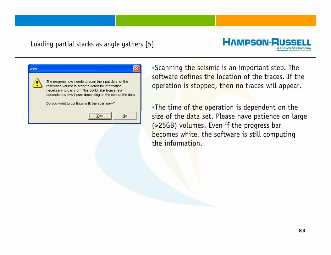
Scanning the seismic is an important step. The software defines the location of the traces. If the operation is stopped, then no traces will appear.
The time of the operation is dependent on the size of the data set. Please have patience on large (>25GB) volumes. Even if the progress bar becomes white, the software is still computing the informationthe information.
83
Loading partial stacks as angle gathers [6]g p g g [ ]
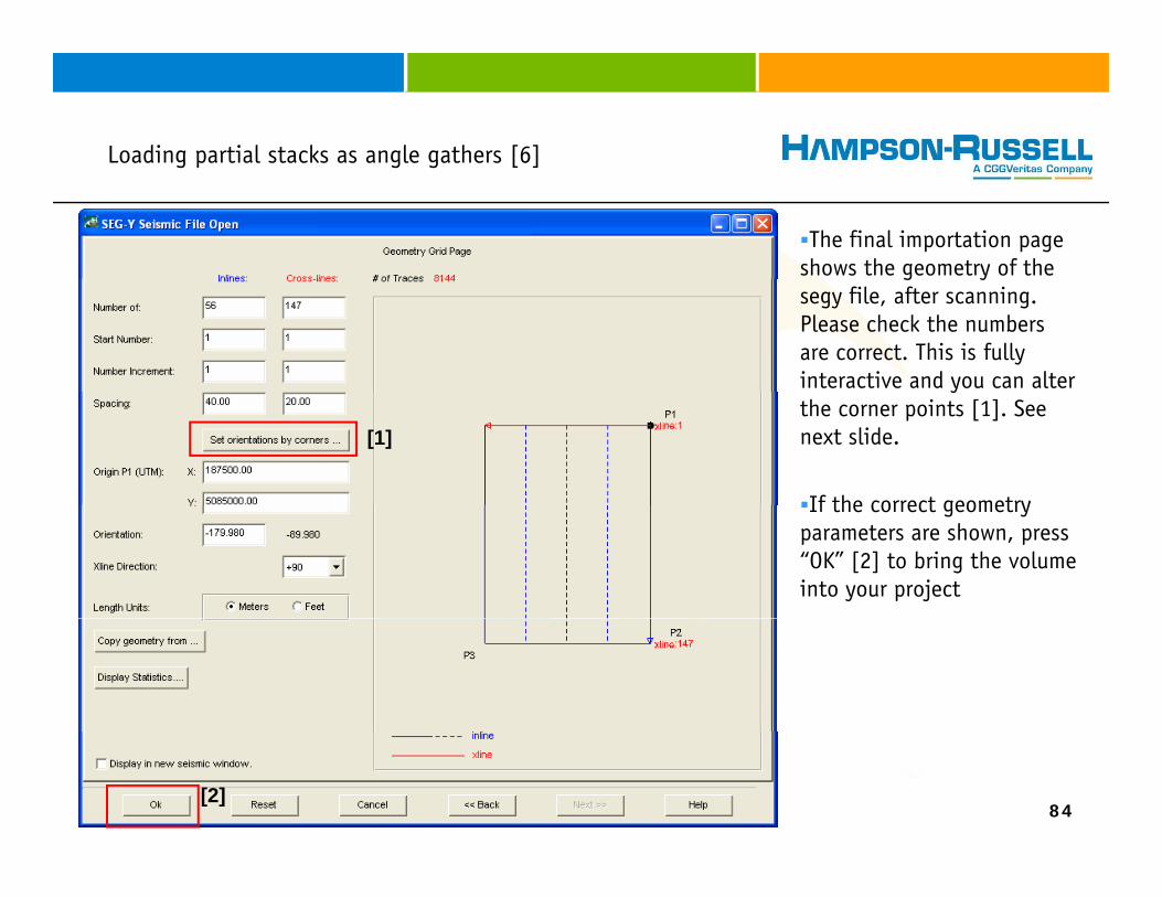
The final importation page shows the geometry of the g ysegy file, after scanning. Please check the numbers are correct. This is fully interactive and you can alter ythe corner points [1]. See next slide.
If the correct geometry
[1]
If the correct geometry parameters are shown, press “OK” [2] to bring the volume into your project
84[2]
Loading partial stacks as angle gathers [7]g p g g [ ]
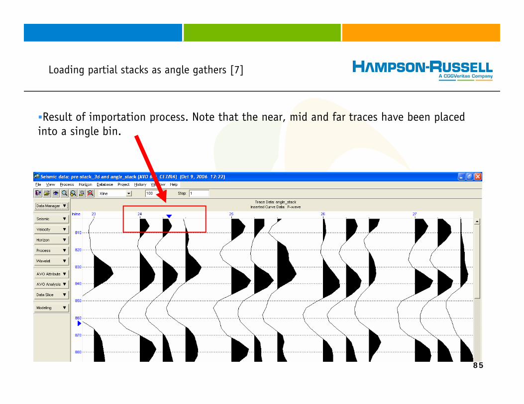
Result of importation process. Note that the near, mid and far traces have been placed into a single bin.
85
Loading partial stacks as angle gathers [8]g p g g [ ]
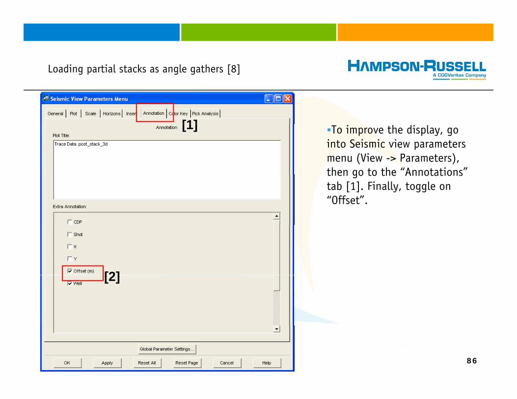
[1] To improve the display, go into Seismic view parameters menu (View -> Parameters), then go to the “Annotations”
[1]
then go to the Annotations tab [1]. Finally, toggle on “Offset”.
[2][2]
86
SeisLoader [1][ ]
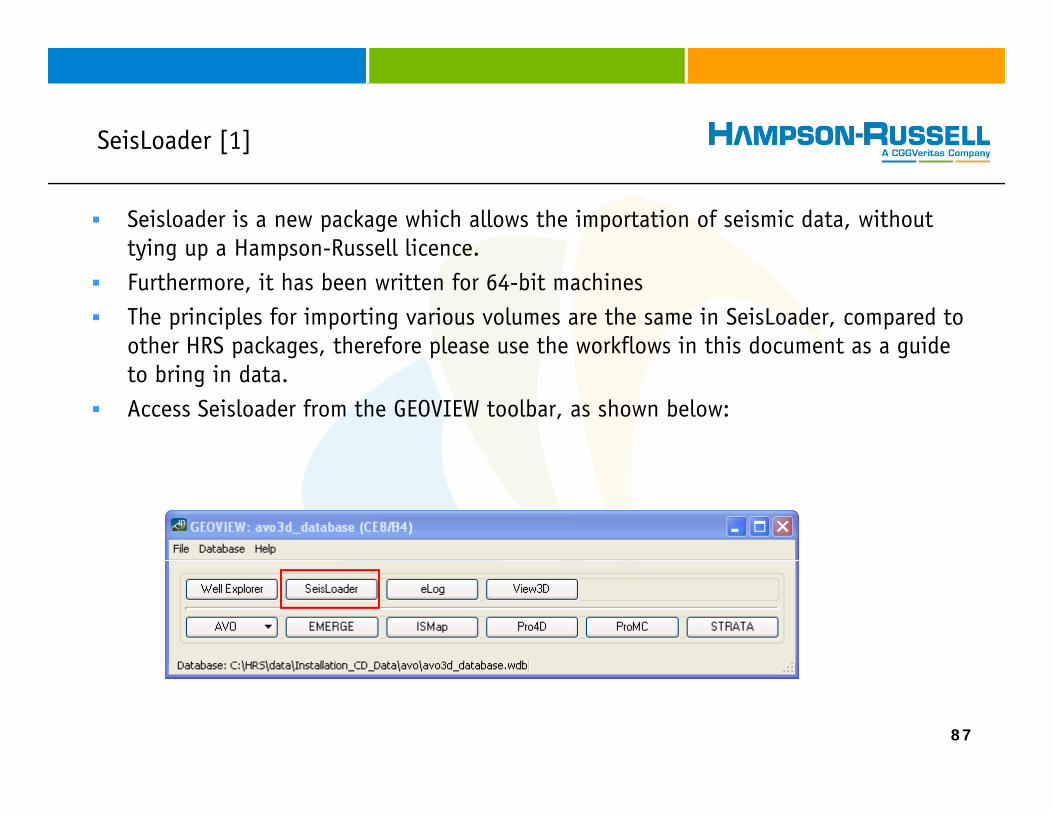
Seisloader is a new package which allows the importation of seismic data, without tying up a Hampson-Russell licence.tying up a Hampson Russell licence.Furthermore, it has been written for 64-bit machinesThe principles for importing various volumes are the same in SeisLoader, compared to other HRS packages, therefore please use the workflows in this document as a guide p g , p gto bring in data.Access Seisloader from the GEOVIEW toolbar, as shown below:
87
SeisLoader [2][ ]
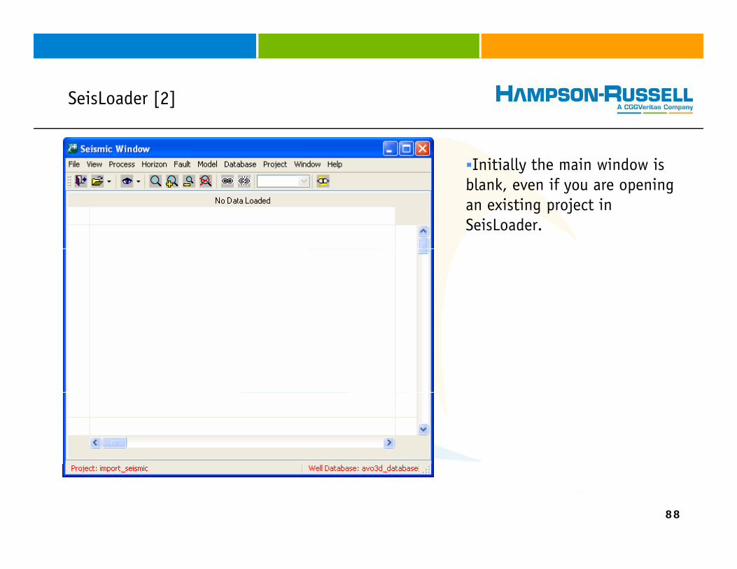
Initially the main window is blank, even if you are opening an existing project in SeisLoader.
88
SeisLoader [3][ ]
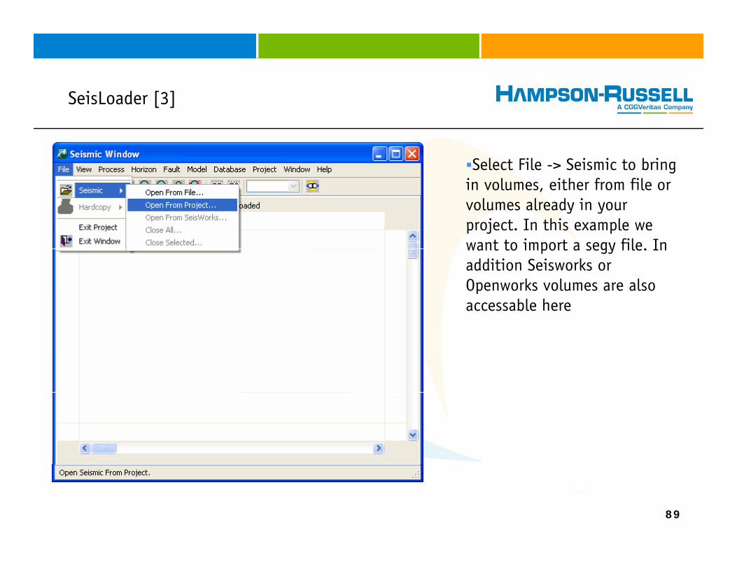
Select File -> Seismic to bring in volumes, either from file or volumes already in your project. In this example we want to import a segy file. Inwant to import a segy file. In addition Seisworks or Openworks volumes are also accessable here
89
SeisLoader [4][ ]
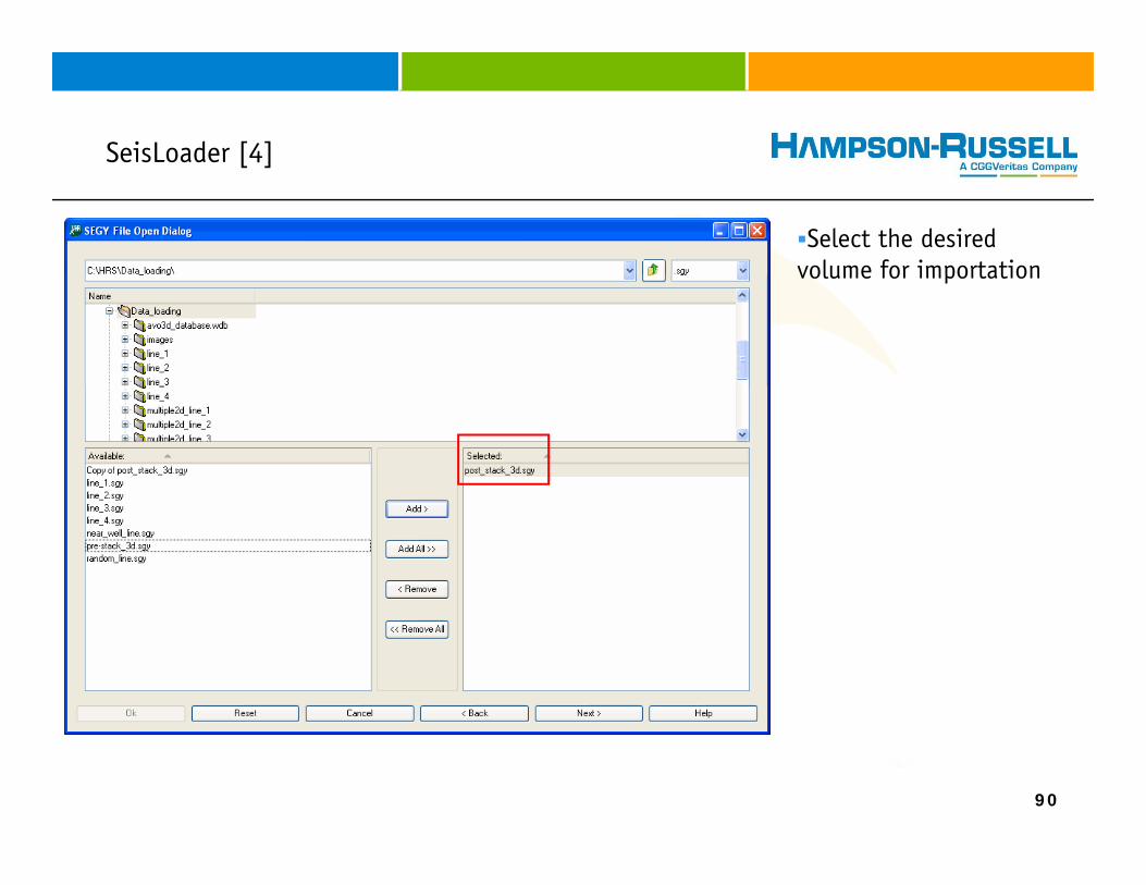
Select the desired volume for importationvolume for importation
90
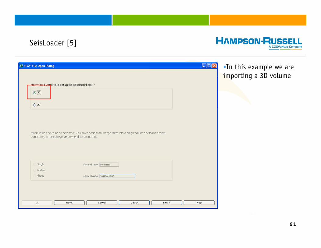
SeisLoader [5][ ]
In this example we are importing a 3D volumeimporting a 3D volume
91
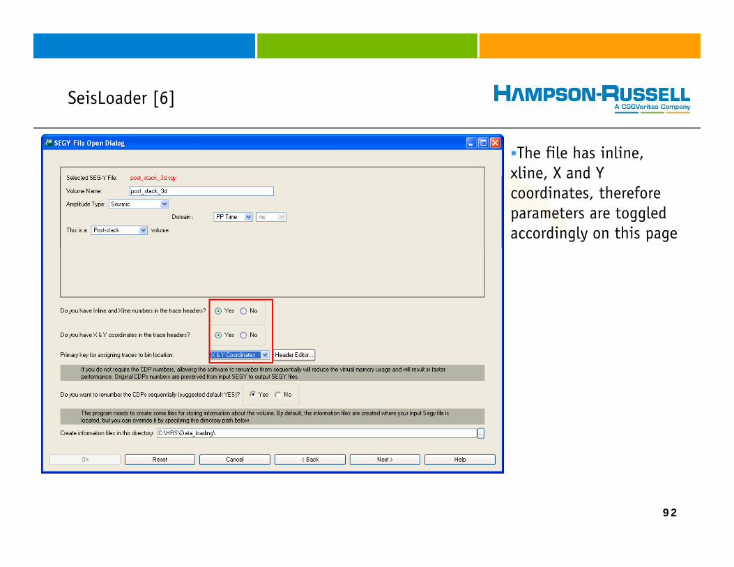
SeisLoader [6][ ]
The file has inline, xline, X and Yxline, X and Y coordinates, therefore parameters are toggled accordingly on this page
92
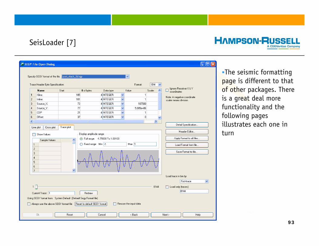
SeisLoader [7][ ]
The seismic formatting page is different to that of other packages. There is a great deal more functionality and thefunctionality and the following pages illustrates each one in turn
93
SeisLoader [8][ ]
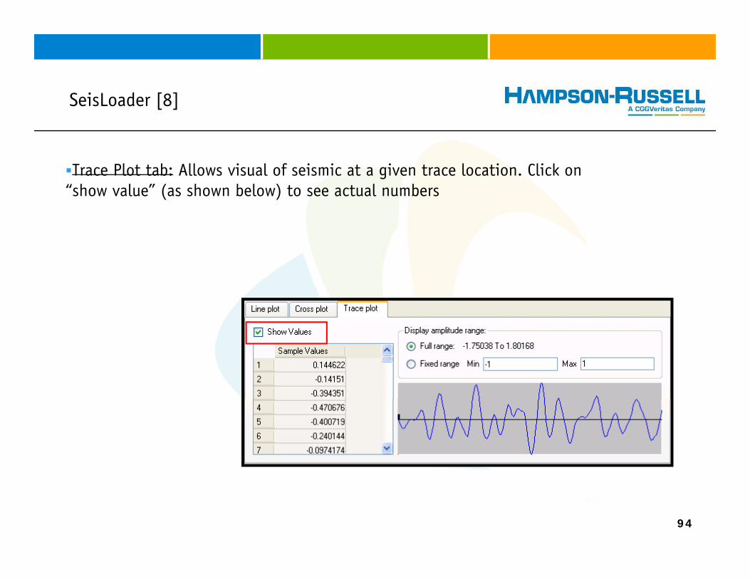
Trace Plot tab: Allows visual of seismic at a given trace location. Click on “show value” (as shown below) to see actual numbers
94
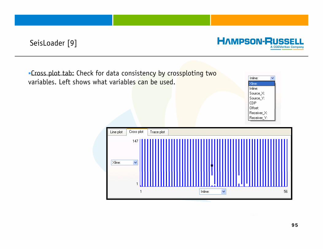
SeisLoader [9][ ]
Cross plot tab: Check for data consistency by crossploting two variables. Left shows what variables can be used.
95
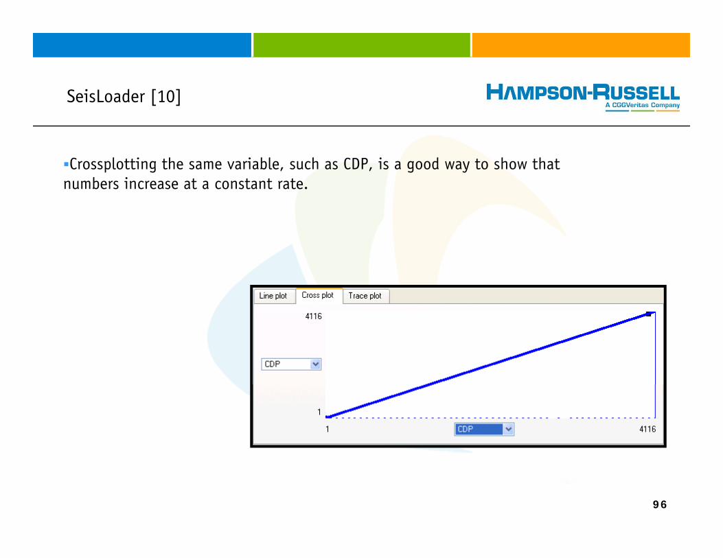
SeisLoader [10][ ]
Crossplotting the same variable, such as CDP, is a good way to show that numbers increase at a constant rate.
96
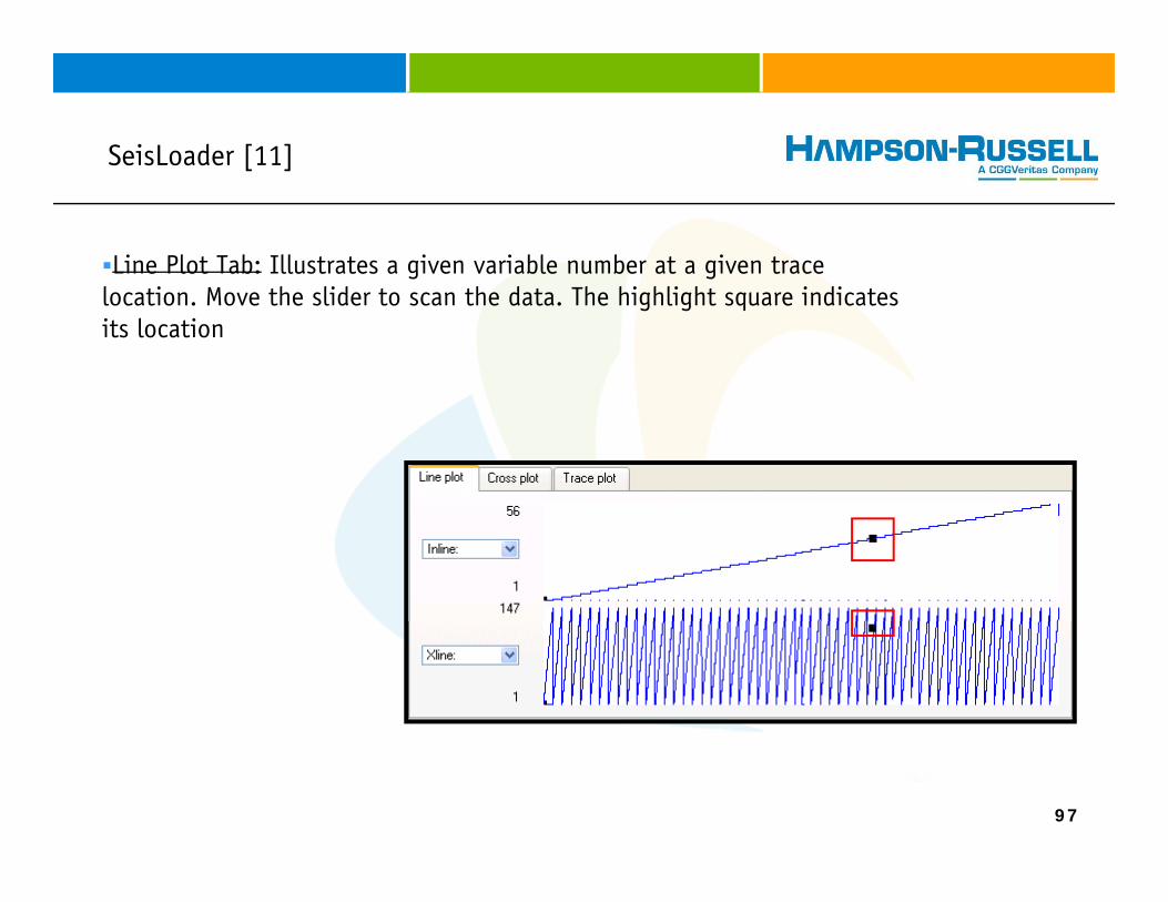
SeisLoader [11][ ]
Line Plot Tab: Illustrates a given variable number at a given trace location. Move the slider to scan the data. The highlight square indicates its location
97
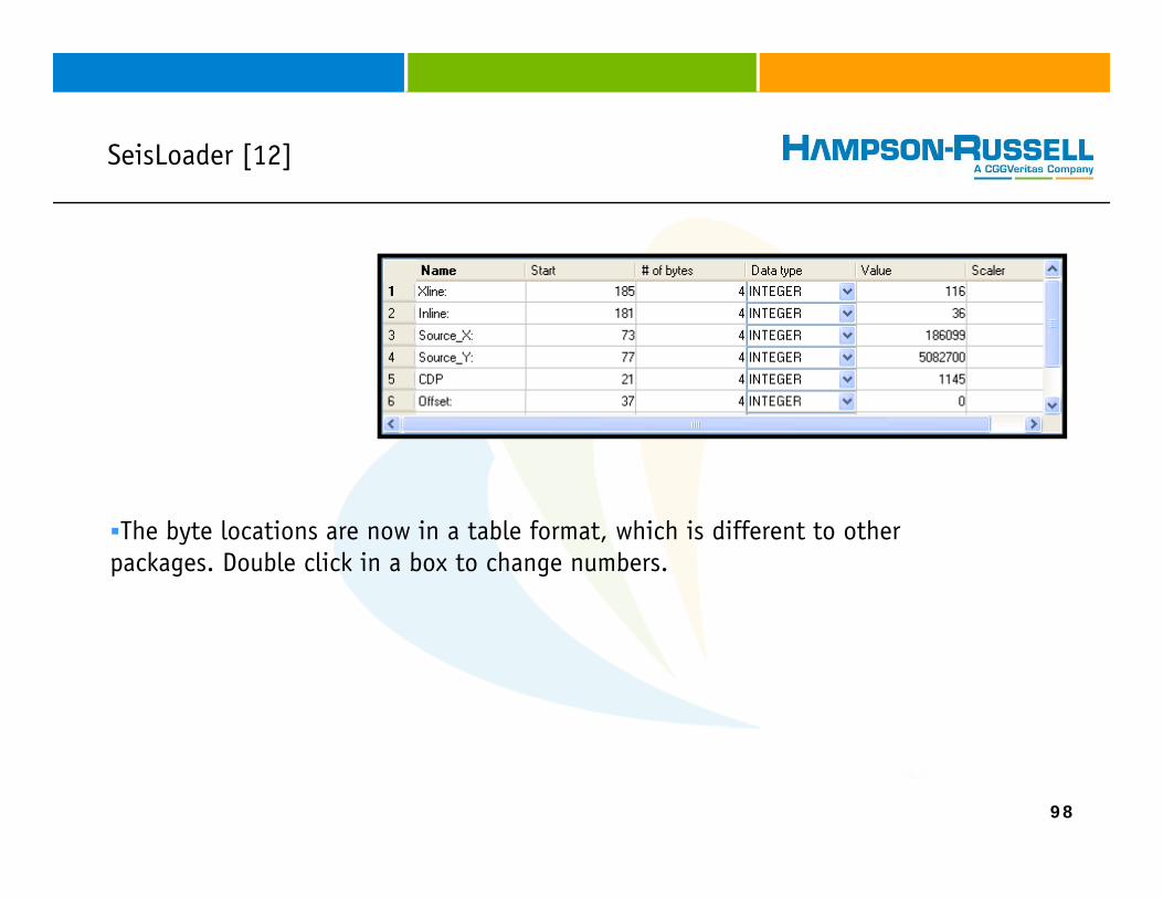
SeisLoader [12][ ]
The byte locations are now in a table format, which is different to other packages. Double click in a box to change numbers.
98
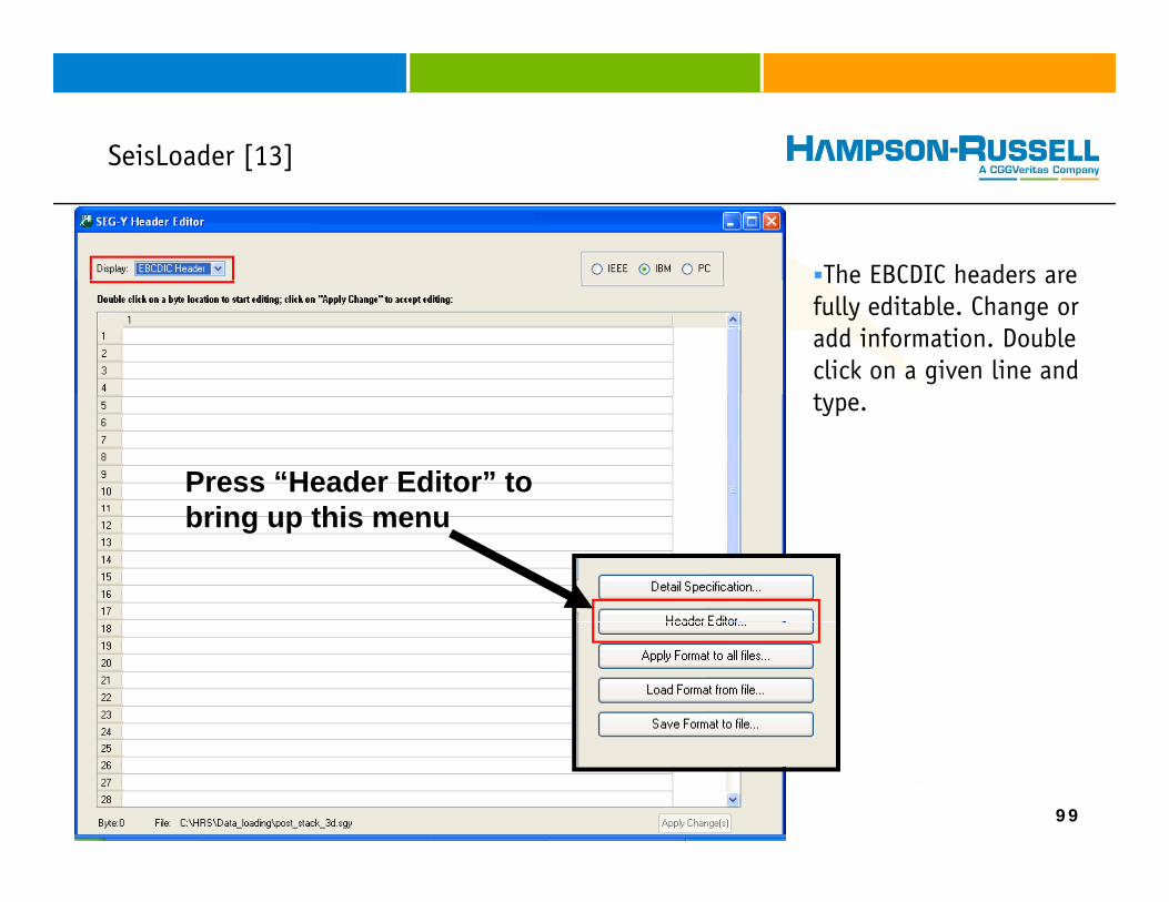
SeisLoader [13][ ]
The EBCDIC headers areThe EBCDIC headers are fully editable. Change or add information. Double click on a given line and ttype.
Press “Header Editor” to b i thibring up this menu
99
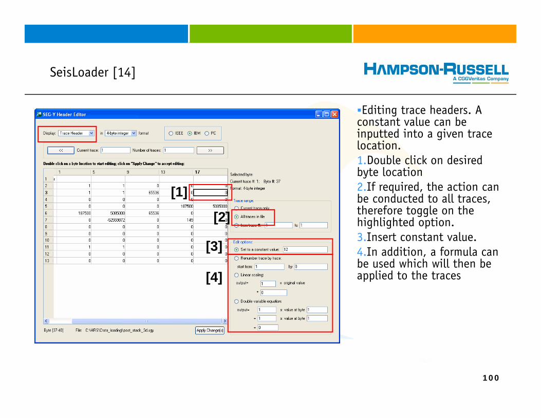
SeisLoader [14][ ]
Editing trace headers. A constant value can be i tt d i t i tinputted into a given trace location.1.Double click on desired byte location2 If i d th ti2.If required, the action can be conducted to all traces, therefore toggle on the highlighted option.3 Insert constant value
[1]
[2]3.Insert constant value.4.In addition, a formula can be used which will then be applied to the traces
[3]
[4]
100
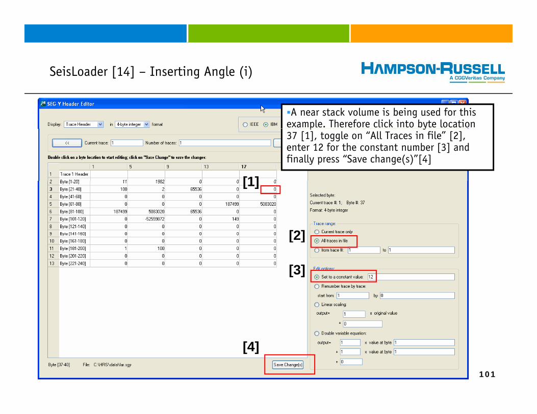
SeisLoader [14] – Inserting Angle (i)[ ] g g ( )
A near stack volume is being used for this example. Therefore click into byte location p y37 [1], toggle on “All Traces in file” [2], enter 12 for the constant number [3] and finally press “Save change(s)”[4]
[1][1]
[2][2]
[3]
101
[4]
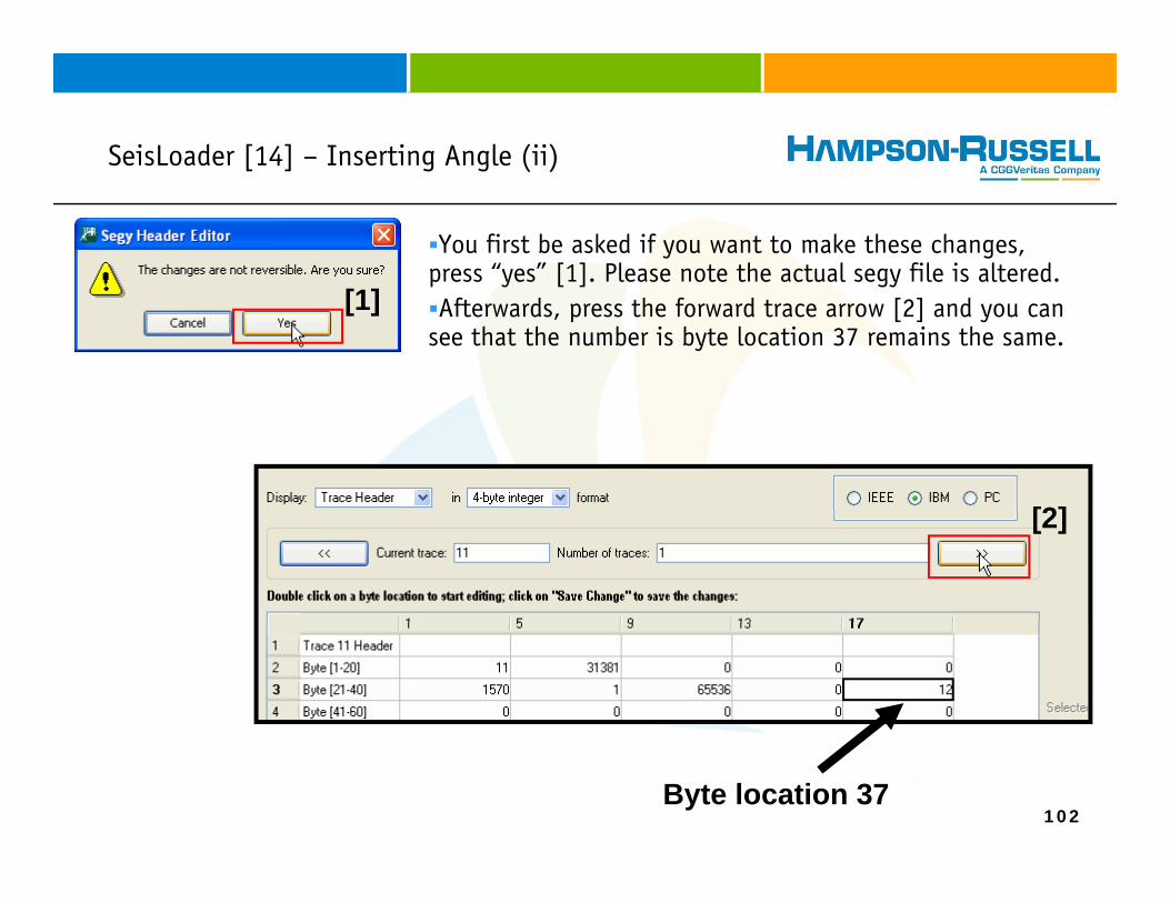
SeisLoader [14] – Inserting Angle (ii)[ ] g g ( )
You first be asked if you want to make these changes, press “yes” [1]. Please note the actual segy file is altered.press yes [1]. Please note the actual segy file is altered. Afterwards, press the forward trace arrow [2] and you can
see that the number is byte location 37 remains the same.[1]
[2][2]
102Byte location 37
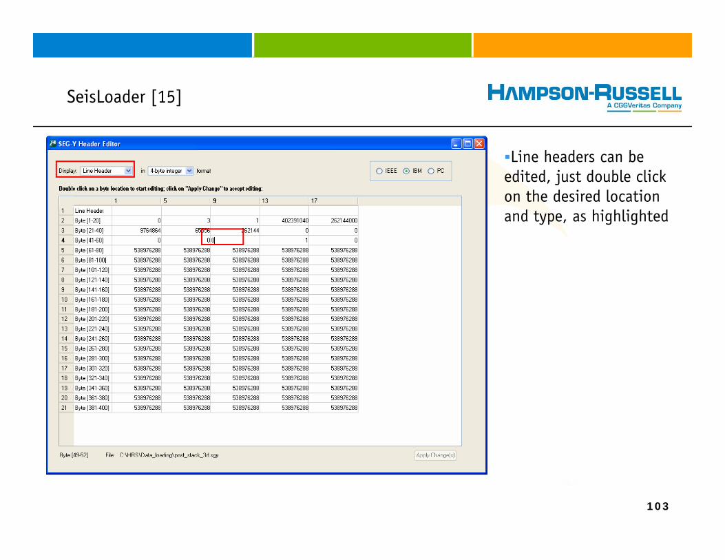
SeisLoader [15][ ]
Line headers can be edited just double clickedited, just double click on the desired location and type, as highlighted
103
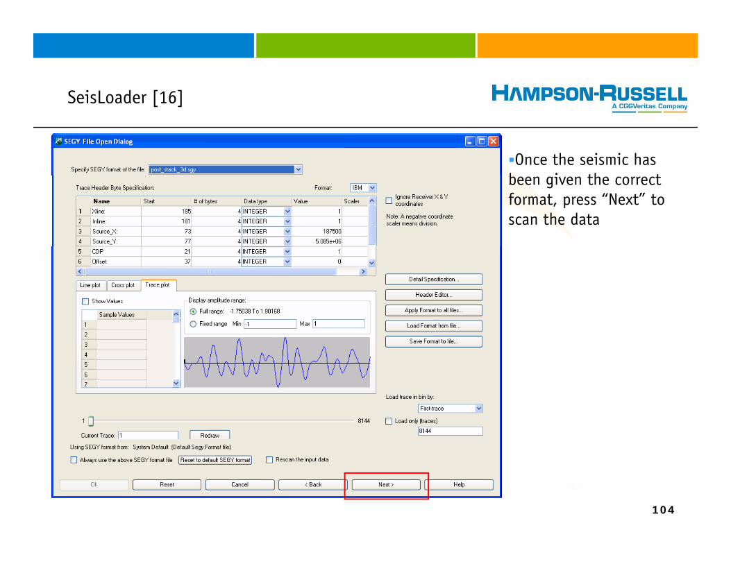
SeisLoader [16][ ]
Once the seismic has b i th tbeen given the correct format, press “Next” to scan the data
104
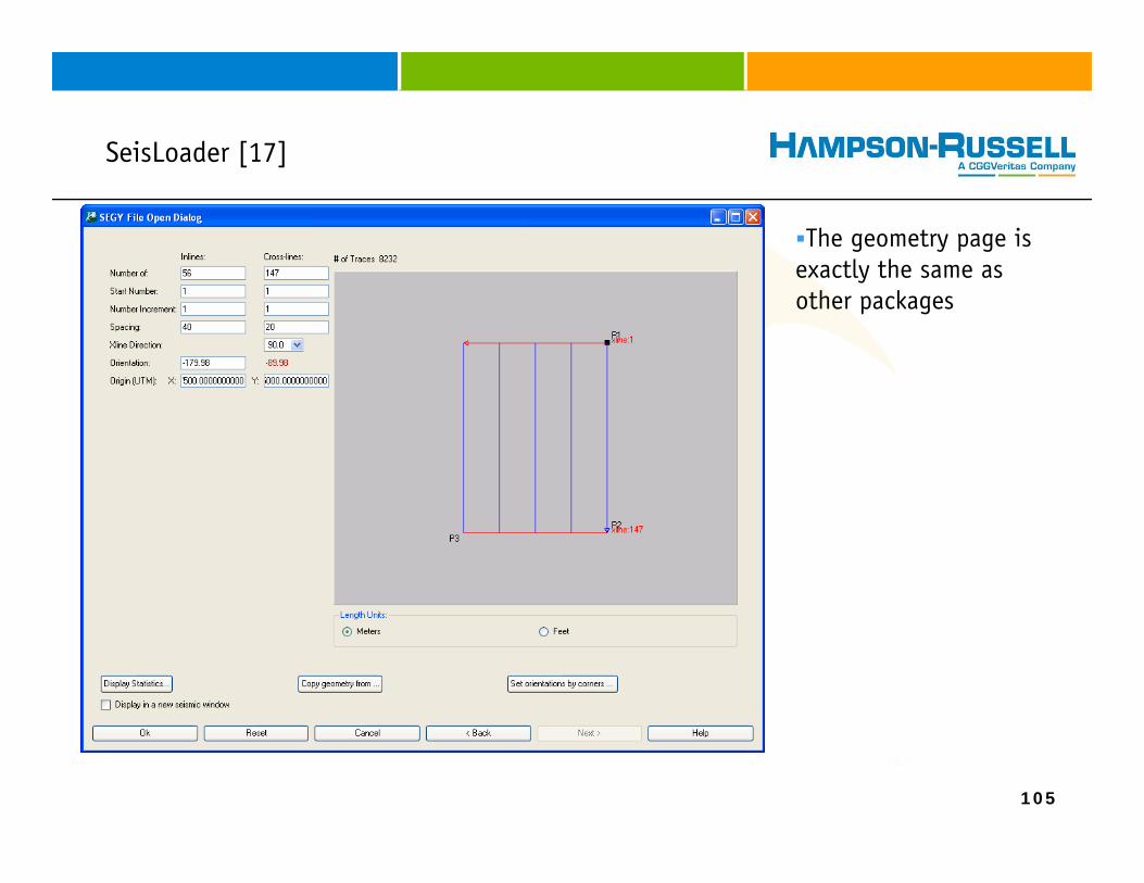
SeisLoader [17][ ]
The geometry page is exactly the same asexactly the same as other packages
105
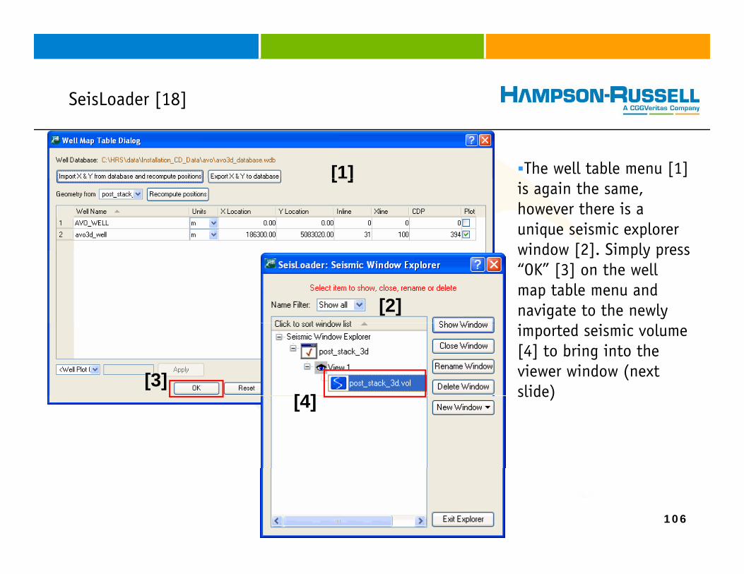
SeisLoader [18][ ]
The well table menu [1] [1]is again the same, however there is a unique seismic explorer window [2] Simply press
[1]
window [2]. Simply press “OK” [3] on the well map table menu and navigate to the newly [2]imported seismic volume [4] to bring into the viewer window (next slide)
[3][4] slide) [4]
106
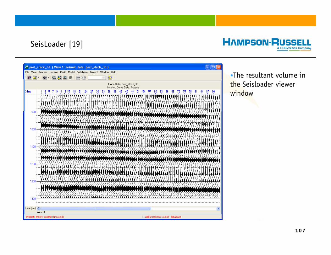
SeisLoader [19][ ]
The resultant volume in the Seisloader viewer window
107
Time-Lapse and Multi-Component Surveys: Introductionp p y
Time-Lapse and Multi-Component surveys are similar in that you typically have two or more seismic volumes that need to have the same geometry in order that differences between the two datasets can be compared.
Oft th i i fil ill d t b “ bi d” i d th t th t f llOften, the seismic files will need to be “rebinned” in order that the geometry of all volumes matches exactly the base survey (or the PP survey for multi-component work). This process can easily be accomplished using the Survey Regrid option in Pro4D and ProMC software.
Pro4D also offers the ability to group the surveys from different vintages into one group to allow for easy comparison. This grouping ability is available in the Data Explorer interface.
ProMC has some slight differences when loading the SEG-Y files. In this case, care b k h h d i (PP PS SS d i ) d h i
108
must be taken that the correct domain (PP, PS or SS domain) and the correct time domain (PP time, PS time or SS time) is entered.
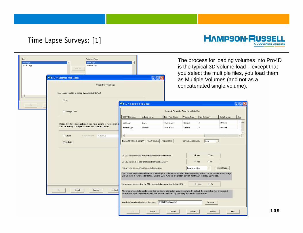
Time Lapse Surveys: [1]p y [ ]
The process for loading volumes into Pro4D is the typical 3D volume load – except that you select the multiple files you load themyou select the multiple files, you load them as Multiple Volumes (and not as a concatenated single volume).
109
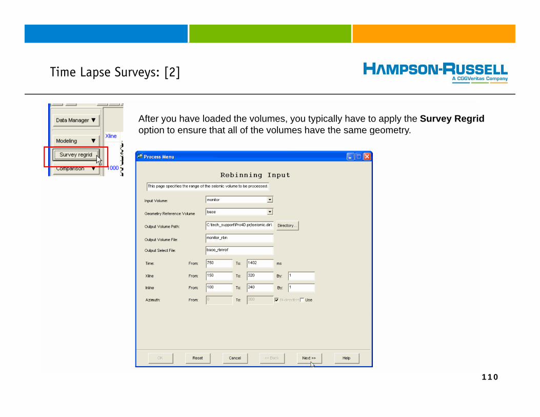
Time Lapse Surveys: [2]p y [ ]
After you have loaded the volumes, you typically have to apply the Survey Regridoption to ensure that all of the volumes have the same geometryoption to ensure that all of the volumes have the same geometry.
110
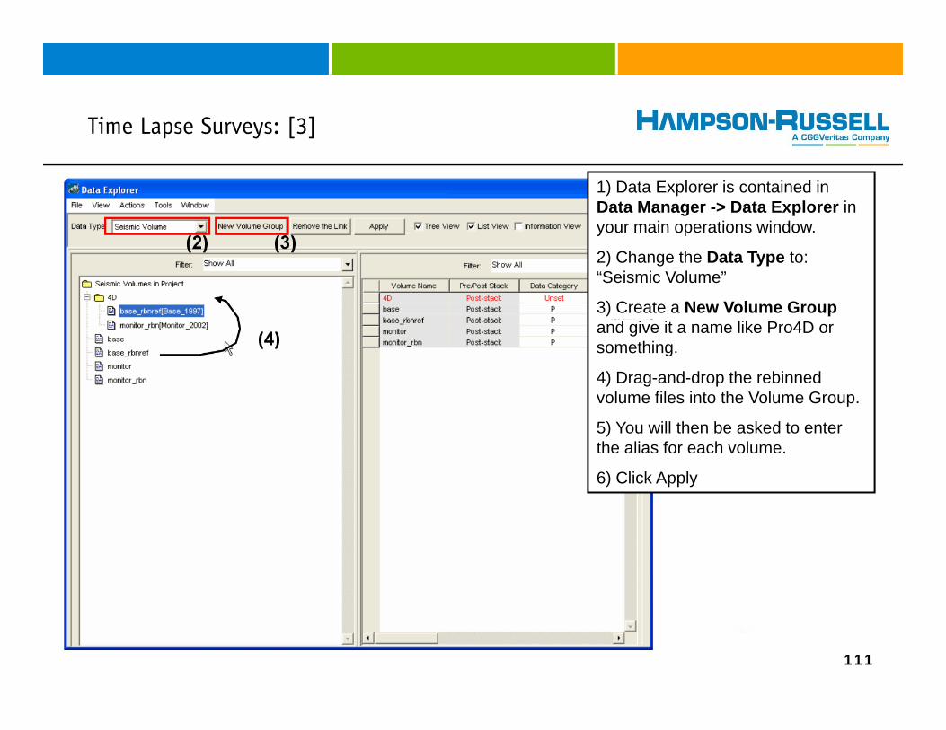
Time Lapse Surveys: [3]
1) Data Explorer is contained in Data Manager -> Data Explorer in your main operations window
p y [ ]
your main operations window.
2) Change the Data Type to: “Seismic Volume”
3) Create a New Volume Groupand give it a name like Pro4D or something.
4) Drag-and-drop the rebinned volume files into the Volume Group.
5) You will then be asked to enter the alias for each volume.
6) Click Apply
111
Time Lapse Surveys: [4]p y [ ]
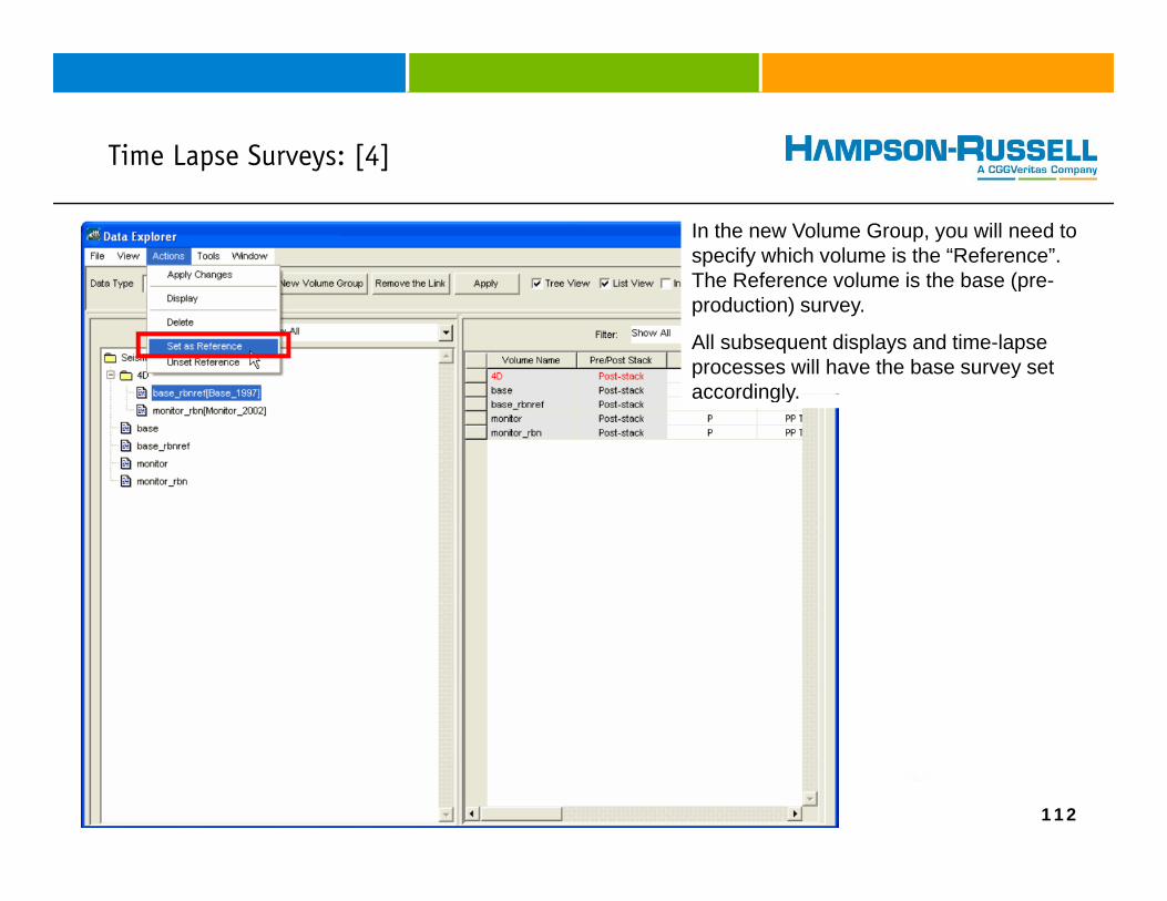
In the new Volume Group, you will need to specify which volume is the “Reference”. The Reference volume is the base (preThe Reference volume is the base (pre-production) survey.
All subsequent displays and time-lapse processes will have the base survey set accordinglyaccordingly.
112
Time-Lapse Surveys: [V]p y [ ]
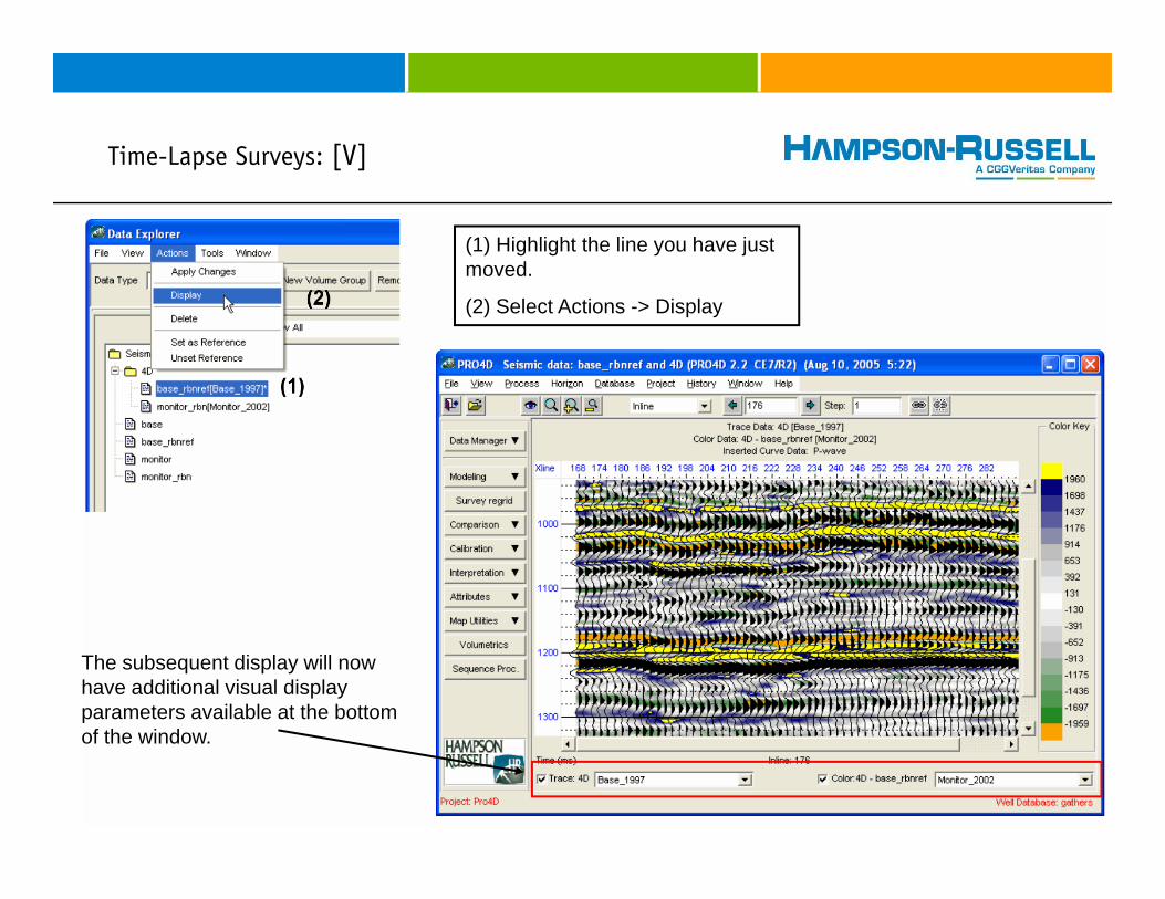
(1) Highlight the line you have just moved.
(2) Select Actions -> Display
The subsequent display will now have additional visual display parameters available at the bottom of the window
113
of the window.

Multi-Component Surveys: [I]p y [ ]
The process for loading volumes into ProMC is the typical 3D volume load –except that you select the multiple files, you y yload them as Multiple Volumes (and not as a concatenated single volume).
114
Multi-Component Surveys: [II]p y [ ]
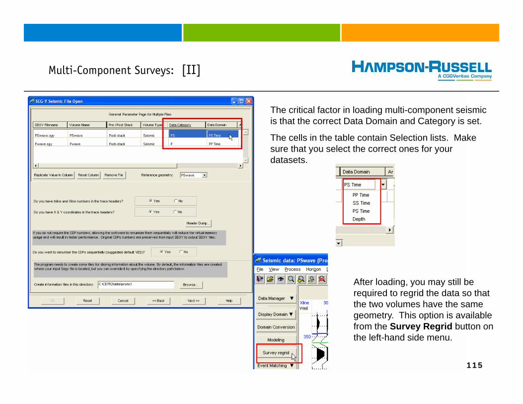
The critical factor in loading multi-component seismic is that the correct Data Domain and Category is set.g y
The cells in the table contain Selection lists. Make sure that you select the correct ones for your datasets.
Aft l di till bAfter loading, you may still be required to regrid the data so that the two volumes have the same geometry. This option is available from the Survey Regrid button on
115
y gthe left-hand side menu.