In

Encylopedia of Electrical and Electronic Engineering, John Wiley and Sons.

Data Structures and Algorithms

Panos M. Pardalos1 and Sanguthevar Rajasekaran2

Abstract

In this article we provide an introduction to data structures and algorithms.We consider some basic data structures and deal with implementations of adictionary and a priority queue. Algorithms for such basic problems as matrixmultiplication, binary search, sorting, and selection are given. The concepts ofrandomized computing and parallel computing are also visited.

1 Preliminaries

By an algorithm we mean any technique that can be used to solve a given problem.

The problem under concern could be that of rearranging a given sequence of numbers,

solving a system of linear equations, finding the shortest path between two nodes

in a graph, etc. An algorithm consists of a sequence of basic operations such as

addition, multiplication, comparison, and so on and is typically described in a machine

independent manner. When an algorithm gets coded in a specified programming

language such as C, C++, or Java, it becomes a program that can be executed on a

computer.

For any given problem, there could possibly be many different techniques that

solve it. Thus it becomes necessary to define performance measures that can be used

to judge different algorithms. Two popular measures are the time complexity and the

space complexity.

The time complexity or the run time of an algorithm refers to the total number of

basic operations performed in the algorithm. As an example, consider the problem

of finding the minimum of n given numbers. This can be accomplished using n − 1

comparisons. Of the two measures perhaps time complexity is more important. This

measure is useful for the following reasons. 1) We can use the time complexity of an

algorithm to predict its actual run time when it is coded in a programming language

and run on a specific machine. 2) Given several different algorithms for solving the

same problem we can use their run times to identify the best one.

1Dept. of ISE, Univ. of Florida2Dept. of CISE, Univ. of Florida. This work is supported in part by an NSF Award CCR-95-

03-007 and an EPA Grant R-825-293-01-0.

1

The space complexity of an algorithm is defined to be the amount of space (i.e.,

the number of memory cells) used by the algorithm. This measure can be critical

especially when the input data itself is huge.

We define the input size of a problem instance to be the amount of space needed

to specify the instance. For the problem of finding the minimum of n numbers, the

input size is n, since we need n memory cells, one for each number, to specify the

problem instance. For the problem of multiplying two n× n matrices, the input size

is 2n2, because there are these many elements in the input.

Both the run time and the space complexity of an algorithm are expressed as

functions of the input size.

For any given problem instance, its input size alone may not be enough to decide

its time complexity. To illustrate this point, consider the problem of checking if an

element x is in an array a[1 : n]. This problem is called the searching problem. One

way of solving this problem is to check if x = a[1]; if not check if x = a[2]; and so on.

This algorithm may terminate after the first comparison, after the second comparison,

. . ., or after comparing x with every element in a[ ]. Thus it is necessary to qualify the

time complexity as the best case, the worst case, the average case, etc. The average

case run time of an algorithm is the average run time taken over all possible inputs

(of a given size).

Analysis of an algorithm can be simplified using asymptotic functions such as

O(.), Ω(.), etc. Let f(n) and g(n) be nonnegative integer functions of n. We say

f(n) is O(g(n)) if f(n) ≤ c g(n) for all n ≥ n0 where c and n0 are some constants.

Also, we say f(n) = Ω(g(n)) if f(n) ≥ c g(n) for all n ≥ n0 for some constants c and

n0. If f(n) = O(g(n)) and f(n) = Ω(g(n)), then we say f(n) = Θ(g(n)). Usually

we express the run times (or the space complexities) of algorithms using Θ( ). The

algorithm for finding the minimum of n given numbers takes Θ(n) time.

An algorithm designer is faced with the task of developing the best possible algo-

rithm (typically an algorithm whose run time is the best possible) for any given prob-

lem. Unfortunately, there is no standard recipe for doing this. Algorithm researchers

have identified a number of useful techniques such as the divide-and-conquer, dy-

namic programming, greedy, backtracking, and branch-and-bound. Application of

any one or a combination of these techniques by itself may not guarantee the best

possible run time. Some innovations (small and large) may have to be discovered and

incorporated.

Note: All the logarithms used in this article are to the base 2, unless otherwise

mentioned.

2

2 Data Structures

An algorithm can be thought of as a mapping from the input data to the output data.

A data structure refers to the way the data is organized. Often the choice of the data

structure determines the efficiency of the algorithm using it. Thus the study of data

structures plays an essential part in the domain of algorithms design.

Examples of basic data structures include queues, stacks, etc. More advanced

data structures are based on trees. Any data structure supports certain operations

on the data. We can classify data structures depending on the operations supported.

A dictionary supports Insert, Delete, and Search operations. On the other hand a

priority queue supports Insert, Delete-Min, and Find-Min operations. The operation

Insert refers to inserting an arbitrary element into the data structure. Delete refers

to the operation of deleting a specified element. Search takes as input an element x

and decides if x is in the data structure. Delete-Min deletes and returns the minimum

element from the data structure. Find-Min returns the minimum element from the

data structure.

2.1 Queues and Stacks

In a queue, two operations are supported, namely, insert and delete. The operation

insert is supposed to insert a given element into the data structure. On the other hand,

delete deletes the first element inserted into the data structure. Thus a queue employs

the First-In-First-Out policy. A stack also supports insert and delete operations but

uses the Last-In-First-Out policy.

A queue or a stack can be implemented easily using an array of size n, where n is

the maximum number of elements that will ever be stored in the data structure. In

this case an insert or a delete can be performed in O(1) time. We can also implement

stacks and queues using linked lists. Even then the operations will only take O(1)

time.

We can also implement a dictionary or a priority queue using an array or a linked

list. For example consider the implementation of a dictionary using an array. At any

given time, if there are n elements in the data structure, these elements will be stored

in a[1 : n]. If x is a given element to be Inserted, it can be stored in a[n + 1]. To

Search for a given x, we scan through the elements of a[ ] until we either find a match

or realize the absence of x. In the worst case this operation takes O(n) time. To

Delete the element x, we first Search for it in a[ ]. If x is not in a[ ] we report so and

quit. On the other hand, if a[i] = x, we move the elements a[i+ 1], a[i+ 2], . . . , a[n]

one position to the left. Thus the Delete operation takes O(n) time.

It is also easy to see that a priority queue can be realized using an array such that

each of the three operations takes O(n) time. The same can be done using a linked

list as well.

3

11

5 3

1

98

12

5

8

3

9

(a) (b)

Figure 1: Examples of binary trees

2.2 Binary Search Trees

We can implement a dictionary or a priority queue in time better than offered by

queues and stacks with the help of binary trees with certain properties.

A binary tree is a set of nodes that is either empty or has a node called the root

and two disjoint binary trees that are called the left and right children of the root.

These children are also called the left and right subtrees, respectively. We store some

data at each node of a binary tree. Figure 1 shows examples of binary trees.

Each node has a label associated with it. We might use the data stored at any

node itself as its label. For example, in Figure 1(a), 5 is the root. 8 is the right child

of 5 and so on. In Figure 1(b), 11 is the root. 5 is the left child of 11. The subtree

containing the nodes 5, 12, and 8 is the left subtree of 11, etc. We can also define

parent relationship in the usual manner. For example, in the tree of Figure 1(a), 5 is

the parent of 8, 8 is the parent of 3, etc. A tree node is called a leaf if it does not

have any children. 9 is a leaf in the tree of Figure 1(a). The nodes 8 and 9 are leaves

in the tree of Figure 1(b).

The level of the root is defined to be 1. The level of any other node is defined to

be + 1, where is the level of its parent. In the tree of Figure 1(b), the level of 3

and 5 is 2; the level of 12 and 1 is 3; and the level of 8 and 9 is 4. The height of a

tree is defined to be the maximum level of any node in the tree. The trees of Figure

1 have a height of 4.

A binary search tree is a binary tree such that the data (or key) stored at any

node is greater than any key in its left subtree and smaller than any key in its right

subtree. Trees in Figure 1 are not binary search trees since for example, in the tree

of Figure 1(a), the right subtree of node 8 has a key 3 that is smaller than 8. Figure

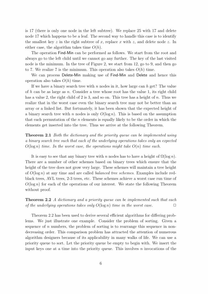
2 has an example of a binary search tree.

We can verify that the tree of Figure 2 is a binary search tree considering each

node of the tree and its subtrees. For the node 12, the keys in its left subtree are 9

and 7 which are smaller. Keys in its right subtree are 25, 17, 30, and 28 which are all

greater than 12. Node 25 has 17 in its left subtree and 30 and 28 in its right subtree,

4

12

9

717

25

30

28

Figure 2: Example of a binary search tree

and so on.

We can implement both a dictionary and a priority queue using binary search

trees. Now we illustrate how to perform the following operations on a binary search

tree: Insert, Delete, Search, Find-Min, and Delete-Min.

To Search for a given element x, we compare x with the key at the root y. If

x = y, we are done. If x < y, then if at all x is in the tree it has to be in the left

subtree. On the other hand, if x > y, x can only be in the right subtree, if at all.

Thus after making one comparison, the searching problem reduces to searching either

the left or the right subtree, i.e., the search space reduces to a tree of height one less.

Thus the total time taken by this search algorithm is O(h), where h is the height of

the tree.

In order to Insert a given element x into a binary search tree, we first search for x

in the tree. If x is already in the tree, we can quit. If not, the search will terminate

in a leaf y such that x can be inserted as a child of y. Look at the binary search tree

of Figure 2. Say we want to insert 19. The Search algorithm begins by comparing

19 with 12 realizing that it should proceed to the right subtree. Next 19 and 25 are

compared to note that the search should proceed to the left subtree. 17 and 19 are

compared next to realize that the search should move to the right subtree. But the

right subtree is empty. This is where the Search algorithm will terminate. The node

17 is y. We can insert 19 as the right child of 17. Thus we see that we can also

process the Insert operation in O(h) time.

A Delete operation can also be processed in O(h) time. Let the element to be

deleted be x. We first Search for x. If x is not in the tree, we quit. If not the Search

algorithm will return the node in which x is stored. There are three cases to consider.

1) The node x is a leaf. This is an easy case – we just delete x and quit. 2) The

node x has only one child y. Let z be the parent of x. We make z the parent of y

and delete x. In Figure 2, if we want to delete 9, we can make 12 the parent of 7 and

delete 9. 3) The node x has two children. There are two ways to handle this case.

The first way is to find the largest key y from the left subtree. Replace the contents

of node x with y and delete node y. Note that the node y can have at most one child.

In the tree of Figure 2, say we desire to delete 25. The largest key in the left subtree

5

is 17 (there is only one node in the left subtree). We replace 25 with 17 and delete

node 17 which happens to be a leaf. The second way to handle this case is to identify

the smallest key z in the right subtree of x, replace x with z, and delete node z. In

either case, the algorithm takes time O(h).

The operation Find-Min can be performed as follows. We start from the root and

always go to the left child until we cannot go any further. The key of the last visited

node is the minimum. In the tree of Figure 2, we start from 12, go to 9, and then go

to 7. We realize 7 is the minimum. This operation also takes O(h) time.

We can process Delete-Min making use of Find-Min and Delete and hence this

operation also takes O(h) time.

If we have a binary search tree with n nodes in it, how large can h get? The value

of h can be as large as n. Consider a tree whose root has the value 1, its right child

has a value 2, the right child of 2 is 3, and so on. This tree has a height of n. Thus we

realize that in the worst case even the binary search tree may not be better than an

array or a linked list. But fortunately, it has been shown that the expected height of

a binary search tree with n nodes is only O(logn). This is based on the assumption

that each permutation of the n elements is equally likely to be the order in which the

elements get inserted into the tree. Thus we arrive at the following Theorem.

Theorem 2.1 Both the dictionary and the priority queue can be implemented using

a binary search tree such that each of the underlying operations takes only an expected

O(logn) time. In the worst case, the operations might take O(n) time each.

It is easy to see that any binary tree with n nodes has to have a height of Ω(logn).

There are a number of other schemes based on binary trees which ensure that the

height of the tree does not grow very large. These schemes will maintain a tree height

of O(logn) at any time and are called balanced tree schemes. Examples include red-

black trees, AVL trees, 2-3 trees, etc. These schemes achieve a worst case run time of

O(logn) for each of the operations of our interest. We state the following Theorem

without proof.

Theorem 2.2 A dictionary and a priority queue can be implemented such that each

of the underlying operations takes only O(logn) time in the worst case.

Theorem 2.2 has been used to derive several efficient algorithms for differing prob-

lems. We just illustrate one example. Consider the problem of sorting. Given a

sequence of n numbers, the problem of sorting is to rearrange this sequence in non-

decreasing order. This comparison problem has attracted the attention of numerous

algorithm designers because of its applicability in many walks of life. We can use a

priority queue to sort. Let the priority queue be empty to begin with. We insert the

input keys one at a time into the priority queue. This involves n invocations of the

6

Insert operation and hence will take a total of O(n logn) time (c.f. Theorem 2.2). Fol-

lowed by this we apply Delete-Min n times, to read out the keys in sorted order. This

will take another O(n logn) time as well. Thus we have an O(n logn)-time sorting

algorithm.

3 Algorithms for Some Basic Problems

In this section we deal with some basic problems such as matrix multiplication, binary

search, etc.

3.1 Matrix Multiplication

Matrix multiplication plays a vital role in many areas of science and engineering.

Given two n × n matrices A and B, the problem is to compute C = AB. By

definition, C[i, j] =∑n

k=1A[i, k] ∗ B[k, j]. Using this definition, each element of C

can be computed in Θ(n) time and since there are n2 elements to compute, C can be

computed in Θ(n3) time. This algorithm can be specified as follows.

7

for i := 1 to n do

for j := 1 to n do

C[i, j] := 0;

for k := 1 to n do

C[i, j] := C[i, j] + A[i, k] ∗B[k, j];

One of the most popular techniques used for developing (both sequential and

parallel) algorithms is the divide-and-conquer. The idea is to partition the given

problem into k (for some k ≥ 1) sub-problems, solve each sub-problem, and combine

these partial solutions to arrive at a solution to the original problem. It is natural

to describe any algorithm based on divide-and-conquer as a recursive algorithm (i.e.,

and algorithm that calls itself). The run time of the algorithm will be expressed as

a recurrence relation which upon solution will indicate the run time as a function of

the input size.

Strassen has developed an elegant algorithm based on the divide-and-conquer

technique that can multiply two n × n matrices in Θ(nlog2 7) time. This algorithm

is based on the critical observation that two 2 × 2 scalar matrices can be multiplied

using only seven scalar multiplications (and 18 additions – the asymptotic run time

of the algorithm is oblivious to this number). Partition A and B into submatrices of

size n2× n

2each as shown.

A =

[A11 A12

A21 A22

]; B =

[B11 B12

B21 B22

]

Now make use of the formulas developed by Strassen to multiply two 2× 2 scalar

matrices. Here also there will be seven multiplications, but each multiplication in-

volves two n2× n

2submatrices. These multiplications are performed recursively. There

will also be 18 additions (of n2× n

2submatrices). Since two m ×m matrices can be

added in Θ(m2) time, all of these 18 additions only need Θ(n2) time.

If T (n) is the time taken by this divide-and-conquer algorithm to multiply two

n× n matrices, then T (n) satisfies

T (n) = 7T(n

2

)+Θ(n2)

whose solution is T (n) = Θ(nlog2 7).

Cppersmith and Winograd have proposed an algorithm that only takes O(n2.376)

time. This is a complex algorithm details of which can be found in the reference

supplied at the end of this article.

8

3.2 Binary Search

Let a[1 : n] be a given array whose elements are in non-decreasing order and let x

be another element. The problem is to check if x is a member of a[ ]. A simple

divide-and-conquer algorithm can also be designed for this problem.

The idea is to first check if x = a[

n2

]. If so, the problem has been solved. If not,

the search space reduces by a factor of 2. This is because if x > a[

n2

], then x can

only be in the second half of the array if at all. Likewise, if x < a[

n2

], then x can

only be in the first half of the array if at all. If T (n) is the number of comparisons

made by this algorithm on any input of size n, then T (n) satisfies T (n) = T(

n2

)+ 1,

which solves to T (n) = Θ(logn).

4 Sorting

Several optimal algorithms have been developed for sorting. We have already seen

one such algorithm in Section 2.2 that employs priority queues. We assume that the

elements to be sorted are from a linear order. If no other assumptions are made about

the keys to be sorted, the sorting problem will be called general sorting or comparison

sorting. In this section we consider general sorting as well as sorting with additional

assumptions.

4.1 General Sorting

We look at two general sorting algorithms. The first algorithm is called the selection

sort. Let the input numbers be in the array a[1 : n]. We first find the minimum of

these n numbers by scanning through them. This takes n− 1 comparisons. Let this

minimum be in a[i]. We exchange a[1] and a[i]. Next we find the minimum of a[2 : n]

using n− 2 comparisons, and so on.

The total number of comparisons made in the algorithm is (n − 1) + (n − 2) +

· · ·+ 2 + 1 = Θ(n2).

An asymptotically better algorithm can be obtained using divide-and-conquer.

This algorithm is referred to as the merge sort. If the input numbers are in a[1 : n],

we divide the input into two halves, namely a[1 : n

2

]and a

[n2+ 1 : n

]. Sort each half

recursively and finally merge the two sorted subsequences. The problem of merging

is to take as input two sorted sequences and produce a sorted sequence of all the

elements of the two sequences. We can show that two sorted sequences of length l

and m, respectively, can be merged in Θ(l+m) time. Therefore, the two sorted halves

of the array a[ ] can be merged in Θ(n) time.

If T (n) is the time taken by the merge sort on any input of size n, then we have

T (n) = 2T(

n2

)+Θ(n), which solves to T (n) = Θ(n logn).

9

Now we show how to merge two given sorted sequences with l and m elements,

respectively. Let X = q1, q2, . . . , ql and Y = r1, r2, . . . , rm be the sorted (in non-

decreasing order) sequences to be merged. Compare q1 and r1. Clearly, the minimum

of q1 and r1 is also the minimum of X and Y put together. Output this minimum and

delete it from the sequence it came from. In general, at any given time, compare the

current minimum element of X with the current minimum of Y , output the minimum

of these two, and delete the output element from its sequence. Proceed in this fashion

until one of the sequences becomes empty. At this time output all the elements of

the remaining sequence (in order).

Whenever the above algorithm makes a comparison, it outputs one element (either

fromX or from Y ). Thus it follows that the algorithm cannot make more than l+m−1

comparisons.

Theorem 4.1 We can sort n elements in Θ(n logn) time.

It is easy to show that any general sorting algorithm has to make Ω(n log n)

comparisons and hence the merge sort is asymptotically optimal.

4.2 Integer Sorting

We can perform sorting in time better than Ω(n log n) making additional assumptions

about the keys to be sorted. In particular, we assume that the keys are integers in

the range [1, nc], for any constant c. This version of sorting is called integer sorting.

In this case, sorting can be done in Θ(n) time.

We begin by showing that n integers in the range [1, m] can be sorted in time

Θ(n + m) for any integer m. We make use of an array a[1 : m] of m lists, one for

each possible value that a key can have. These lists are empty to begin with. Let

X = k1, k2, . . . , kn be the input sequence. We look at each input key and put it in

an appropriate list of a[ ]. In particular, we append key ki to the end of list a[ki], for

i = 1, 2, . . . , n. This takes Θ(n) time. We have basically grouped the keys according

to their values.

Next, we output the keys of list a[1], the keys of list a[2], and so on. This takes

Θ(m+ n) time. Thus the whole algorithm runs in time Θ(m+ n).

If one uses this algorithm (called the bucket sort) to sort n integers in the range

[1, nc] for c > 1, the run time will be Θ(nc). This may not be acceptable since we can

do better using the merge sort.

We can sort n integers in the range [1, nc] in Θ(n) time using the bucket sort and

the notion of radix sorting. Say we are interested in sorting n two-digit numbers. One

way of doing this is to sort the numbers with respect to their least significant digits

and then to sort with respect to their most significant digits. This approach works

provided the algorithm used to sort the numbers with respect to a digit is stable. We

10

say a sorting algorithm is stable if equal keys remain in the same relative order in the

output as they were in the input. Note that the bucket sort as described above is

stable.

If the input integers are in the range [1, nc], we can think of each key as a c logn-

bit binary number. We can conceive of an algorithm where there are c stages. In

stage i, the numbers are sorted with respect to their ith most significant logn-bits.

This means that in each stage we have to sort n log n-bit numbers, i.e., we have to

sort n integers in the range [1, n]. If we use the bucket sort in every stage, the stage

will take Θ(n) time. Since there are only a constant number of stages, the total run

time of the algorithm is Θ(n). We get the following Theorem.

Theorem 4.2 We can sort n integers in the range [1, nc] in Θ(n) time for any con-

stant c.

5 Selection

In this section we consider the problem of selection. We are given a sequence of n

numbers and we are supposed to identify the ith smallest number from out of these,

for a specified i, 1 ≤ i ≤ n. For example if i = 1, we are interested in finding the

smallest number. If i = n, we are interested in finding the largest element.

A simple algorithm for this problem could pick any input element k, partition the

input into two – the first part being those input elements that are less than x and the

second part consisting of input elements greater than x, identify the part that contains

the element to be selected, and finally recursively perform an appropriate selection in

the part containing the element of interest. This algorithm can be shown to have an

expected (i.e., average case) run time of O(n). In general the run time of any divide-

and-conquer algorithm will be the best if the sizes of the subproblems are as even as

possible. In this simple selection algorithm, it may happen so that one of the two

parts is empty at each level of recursion. The second part may have n− 1 elements.

If T (n) is the run time corresponding to this input, then, T (n) = T (n − 1) + Ω(n).

This solves to T (n) = Ω(n2). In fact if the input elements are already in sorted order

and we always pick the first element of the array as the partitioning element, then

the run time will be Ω(n2).

So, even though this simple algorithm has a good average case run time, in the

worst case it can be bad. We will be better off using the merge sort. It is possible

to design an algorithm that can select in Θ(n) time in the worst case, as has been

shown by Blum, Floyd, Pratt, Rivest, and Tarjan.

Their algorithm employs a primitive form of “deterministic sampling”. Say we

are given n numbers. We group these numbers such that there are five numbers in

each group. Find the median of each group. Find also the median M of these group

medians. We can expect M to be an “approximate median” of the n numbers.

11

For simplicity assume that the input numbers are distinct. The median of each

group can be found in Θ(1) time and hence all the medians (excepting for M) can

be found in Θ(n) time. Having found M , we partition the input into two parts X1

and X2. X1 consists of all the input elements that are less than M and X2 contains

all the elements greater than M . This partitioning can also be done in Θ(n) time.

We can also count the number of elements in X1 and X2 within the same time. If

|X1| = i − 1, then, clearly M is the element to be selected. If |X1| ≥ i, then the

element to be selected belongs to X1. On the other hand if |X1| < i− 1, then the ith

smallest element of the input belongs to X2.

It is easy to see that the size of X2 can be at most 710n. This can be argued

as follows. Let the input be partitioned into the groups G1, G2, . . . , Gn/5 with 5

elements in each part. Assume without loss of generality that every group has exactly

5 elements. There are n10

groups such that their medians are less than M . In each

such group there are at least three elements that are less than M . Therefore, there

are at least 310n input elements that are less than M . This in turn means that the

size of X2 can be at most 710n. Similarly, we can also show that the size of X1 is no

more than 710n.

Thus we can complete the selection algorithm by performing an appropriate se-

lection in either X1 or X2, recursively, depending whether the element to be selected

is in X1 or X2, respectively.

Let T (n) be the run time of this algorithm on any input of size n and for any i.

Then it takes T(

n5

)time to identify the median of medians M . Recursive selection

on X1 or X2 takes no more than T(

710n

)time. The rest of the computations account

for Θ(n) time. Thus T (n) satisfies:

T (n) = T(n

5

)+ T

(7

10n

)+Θ(n)

which solves to T (n) = Θ(n). This can be proved by induction.

Theorem 5.1 Selection from out of n elements can be performed in Θ(n) time.

6 Randomized Algorithms

The performance of an algorithm may not be completely specified even when the

input size is known, as has been pointed out before. Three different measures can

be conceived of: the best case, the worst case, and the average case. Typically, the

average case run time of an algorithm is much smaller than the worst case. For

example, Hoare’s quicksort has a worst case run time of O(n2), whereas its average

case run time is only O(n logn). While computing the average case run time one

assumes a distribution (e.g., uniform distribution) on the set of possible inputs. If

12

this distribution assumption does not hold, then the average case analysis may not

be valid.

Is it possible to achieve the average case run time without making any assump-

tions on the input space? Randomized algorithms answer this question in the affir-

mative. They make no assumptions on the inputs. The analysis done of randomized

algorithms will be valid for all possible inputs. Randomized algorithms obtain such

performances by introducing randomness into the algorithms themselves.

Coin flips are made to make certain decisions in randomized algorithms. A ran-

domized algorithm with one possible sequence of outcomes for the coin flips can be

thought of as being different from the same algorithm with a different sequence of

outcomes for the coin flips. Thus a randomized algorithm can be viewed as a family

of algorithms. Some of the algorithms in this family might have a ‘poor performance’

on a given input. It should be ensured that, for any input, the number of algorithms

in the family bad on this input is only a small fraction of the total number of algo-

rithms. If we can find at least (1− ε) (ε being very close to 0) portion of algorithms

in the family that will have a ‘good performance’ on any given input, then clearly,

a random algorithm in the family will have a ‘good performance’ on any input with

probability ≥ (1 − ε). We say, in this case, that this family of algorithms (or this

randomized algorithm) has a ‘good performance’ with probability ≥ (1 − ε). ε is

referred to as the error probability. Realize that this probability is independent of the

input distribution.

We can interpret ‘good performance’ in many different ways. Good performance

could mean that the algorithm outputs the correct answer, or its run time is small,

and so on. Different types of randomized algorithms can be conceived of depending

on the interpretation. A Las Vegas algorithm is a randomized algorithm that always

outputs the correct answer but whose run time is a random variable (possibly with

a small mean). A Monte Carlo algorithm is a randomized algorithm that has a

predetermined run time but whose output may be incorrect occasionally.

We can modify asymptotic functions such as O(.) and Ω(.) in the context of

randomized algorithms as follows. A randomized algorithm is said to use O(f(n))

amount of resource (like time, space, etc.) if there exists a constant c such that the

amount of resource used is no more than cαf(n) with probability ≥ 1− n−α on any

input of size n and for any positive α ≥ 1. We can similarly define Ω(f(n)) and

Θ(f(n)) as well. If n is the input size of the problem under concern, then, by high

probability we mean a probability of ≥ 1− n−α for any fixed α ≥ 1.

Illustrative Examples

We provide two examples of randomized algorithms. The first is a Las Vegas algorithm

and the second is a Monte Carlo algorithm.

13

Example 1. [Repeated Element Identification]. Input is an array a[ ] of n elements

wherein there are n− εn distinct elements and εn copies of another element, where ε

is a constant > 0 and < 1. The problem is to identify the repeated element. Assume

without loss of generality that εn is an integer.

Any deterministic algorithm to solve this problem will have to take at least εn+2

time in the worst case. This fact can be proven as follows: Let the input be chosen

by an adversary who has perfect knowledge about the algorithm used. The adversary

can make sure that the first εn+1 elements examined by the algorithm are all distinct.

Therefore, the algorithm may not be in a position to output the repeated element

even after having examined εn + 1 elements. In other words, the algorithm has to

examine at least one more element and hence the claim follows.

We can design a simple O(n) time deterministic algorithm for this problem. Par-

tition the elements such that each part (excepting for possibly one part) has⌈

1ε

⌉+ 1

elements. Then search the individual parts for the repeated element. Clearly, at least

one of the parts will have at least two copies of the repeated element. This algorithm

runs in time Θ(n).

Now we present a simple and elegant Las Vegas algorithm that takes only O(log n)

time. This algorithm is comprised of stages. Two random numbers i and j are picked

from the range [1, n] in any stage. These numbers are picked independently with

replacement. As a result, there is a chance that these two are the same. After picking

i and j we check if i = j and a[i] = a[j]. If so, the repeated element has been found.

If not, the next stage is entered. We repeat the stages as many times as it takes to

arrive at the correct answer.

Lemma 6.1 The above algorithm runs in time O(logn).

Proof: The probability of finding the repeated element in any given stage is P =εn(εn−1)

n2 ≈ ε2. Thus the probability that the algorithm does not find the repeated

element in the first cα loge n (c is a constant to be fixed) stages is

< (1− ε2)cα loge n ≤ n−ε2cα

using the fact that (1−x)1/x ≤ 1/e for any 0 < x < 1. This probability will be < n−α

if we pick c ≥ 1ε2.

I.e., the algorithm takes no more than 1ε2α loge n stages with probability ≥ 1−n−α.

Since each stage takes O(1) time, the run time of the algorithm is O(log n).

Example 2. [Large Element Selection]. Here also the input is an array a[ ] of n

numbers. The problem is to find an element of the array that is greater than the

median. We can assume, without loss of generality, that the array numbers are

distinct and that n is even.

14

Lemma 6.2 The preceding problem can be solved in O(logn) time using a Monte

Carlo algorithm.

Proof: Let the input be X = k1, k2, . . . , kn. We pick a random sample S of size

cα log n from X. This sample is picked with replacement. Find and output the

maximum element of S. The claim is that the output of this algorithm is correct

with high probability.

The algorithm can give an incorrect answer only if all the elements in S have a

value ≤ M , where M is the median. Probability that any element in S is ≤ M is 12.

Therefore, the probability that all the elements of S are ≤M is P =(

12

)cα log n= n−cα.

P will be ≤ n−α if c is picked to be ≥ 1.

In other words, if the sample S has ≥ α logn elements, then the maximum of S

will be a correct answer with probability ≥ (1− n−α).

7 Parallel Computing

One of the ways of solving a given problem quickly is to employ more than one

processor. The basic idea of parallel computing is to partition the given problem into

several subproblems, assign a subproblem to each processor, and put together the

partial solutions obtained by the individual processors.

If P processors are used to solve a problem, then there is a potential of reducing

the run time by a factor of up to P . If S is the best known sequential run time

(i.e., the run time using a single processor), and if T is the parallel run time using

P processors, then PT ≥ S. If not, we can simulate the parallel algorithm using a

single processor and get a run time better than S (which will be a contradiction).

PT is referred to as the work done by the parallel algorithm. A parallel algorithm is

said to be work-optimal if PT = O(S).

In this section we provide a brief introduction to parallel algorithms.

7.1 Parallel Models

The Random Access Machine (RAM) model has been widely accepted as a reasonable

sequential model of computing. In the RAM model, we assume that each of the basic

scalar binary operations such as addition, multiplication, etc. takes one unit of time.

We have assumed this model in our discussion thus far. In contrast, there exist many

well-accepted parallel models of computing. In any such parallel model an individual

processor can still be thought of as a RAM. Variations among different architectures

arise in the ways they implement interprocessor communications. In this article we

categorize parallel models into shared memory models and fixed connection machines.

A shared memory model (also called the Parallel RandomAccess Machine (PRAM))

is a collection of RAMs working in synchrony where communication takes place with

15

the help of a common block of global memory. If processor i has to communicate

with processor j it can do so by writing a message in memory cell j which can then

be read by processor j.

Conflicts for global memory access could arise. Depending on how these conflicts

are resolved, a PRAM can further be classified into three. An Exclusive Read and Ex-

clusive Write (EREW) PRAM does not permit concurrent reads or concurrent writes.

A Concurrent Read and Exclusive Write (CREW) PRAM allows concurrent reads but

not concurrent writes. A Concurrent Read and Concurrent Write (CRCW) PRAM

permits both concurrent reads and concurrent writes. In the case of a CRCW PRAM,

we need an additional mechanism for handling write conflicts, since the processors

trying to write at the same time in the same cell may have different data to write and

a decision has to be made as to which data gets written. Concurrent reads do not

pose such problems, since the data read by different processors will be the same. In

a Common-CRCW PRAM, concurrent writes will be allowed only if the processors

trying to access the same cell have the same data to write. In an Arbitrary-CRCW

PRAM, if more than one processor tries to write in the same cell at the same time,

an arbitrary one of them succeeds. In a Priority-CRCW PRAM, write conflicts are

resolved using priorities assigned to the processors.

A fixed connection machine can be represented as a directed graph whose nodes

represent processors and whose edges represent communication links. If there is an

edge connecting two processors, they can communicate in one unit of time. If two

processors not connected by an edge want to communicate they can do so by sending

a message along a path that connects the two processors. We can think of each

processor in a fixed connection machine as a RAM. Examples of fixed connection

machines are the mesh, the hypercube, the star graph, etc.

Our discussion on parallel algorithms is confined to PRAMs owing to their sim-

plicity.

7.2 Boolean Operations

The first problem considered is that of computing the boolean OR of n given bits.

With n Common-CRCW PRAM processors, we can compute the boolean OR in

O(1) time as follows. The input bits are stored in common memory (one bit per cell).

Every processor is assigned an input bit. We employ a common memory cell M that

is initialized to zero. All the processors that have ones try to write a one in M in one

parallel write step. The result is ready in M after this write step. Using a similar

algorithm, we can also compute the boolean AND of n bits in O(1) time.

Lemma 7.1 The boolean OR or boolean AND of n given bits can be computed in

O(1) time using n Common-CRCW PRAM processors.

16

The different versions of the PRAM form a hierarchy in terms of their computing

power. EREW PRAM, CREW PRAM, Common-CRCW PRAM, Arbitrary-CRCW

PRAM, Priority-CRCW PRAM is an ordering of some of the PRAM versions. Any

model in the sequence is strictly less powerful than any to its right, and strictly more

powerful than any to its left. As aresult, for example, any algorithm that runs on

the EREW PRAM will run on the Common-CRCW PRAM preserving the processor

and time bounds, but the converse may not be true.

7.3 Finding the Maximum

Now we consider the problem of finding the maximum of n given numbers. We

describe an algorithm that can solve this in O(1) time using n2 common CRCW

PRAM processors.

Partition the processors so that there are n processors in each group. Let the

input be k1, k2, . . . , kn and let the groups be G1, G2, . . . , Gn. Processor i is assigned

the key ki. Gi is in-charge of checking if ki is the maximum. In one parallel step,

processors of group Gi compare ki with every input key. In particular processor j of

group Gi computes the bit bij = ki ≥ kj. The bits bi1, bi2, . . . , bin are ANDed using

the algorithm of Lemma 7.1. This can be done in O(1) time. If Gi computes a one

in this step, then one of the processors in Gi outputs ki as the answer.

Lemma 7.2 The maximum (or minimum) of n given numbers can be computed in

O(1) time using n2 common CRCW PRAM processors.

7.4 Prefix Computation

Prefix computation plays a vital role in the design of parallel algorithms. This is as

basic as any arithmetic operation in sequential computing. Let ⊕ be any associative

unit-time computable binary operator defined in some domain Σ. Given a sequence

of n elements k1, k2, . . . , kn from Σ, the problem of prefix computation is to compute

k1, k1⊕k2, k1⊕k2⊕k3, . . . , k1⊕k2⊕· · ·⊕kn. Examples of⊕ are addition, multiplication,

and min. Example of Σ are the set of integers, the set of reals, etc. The prefix sums

computation refers to the special case when ⊕ is addition. The results themselves are

called prefix sums.

Lemma 7.3 We can perform prefix computation on a sequence of n elements in

O(logn) time using n CREW PRAM processors.

Proof. We can use the following algorithm. If n = 1, the problem is solved easily.

If not, the input elements are partitioned into two halves. Solve the prefix com-

putation problem on each half recursively assigning n2processors to each half. Let

y1, y2, . . . , yn/2 and yn/2+1, yn/2+2, . . . , yn be the prefix values of the two halves.

17

There is no need to modify the values y1, y2, . . ., and yn/2 and hence they can

be output as such. Prefix values from the second half can be modified as yn/2 ⊕yn/2+1, yn/2 ⊕ yn/2+2, . . . , yn/2 ⊕ yn. This modification can be done in O(1) time usingn2processors. These n

2processors first read yn/2 concurrently and then update the

second half (one element per processor).

Let T (n) be the time needed to perform prefix computation on n elements using

n processors. T (n) satisfies T (n) = T (n/2) +O(1), which solves to T (n) = O(logn).

The processor bound of the preceding algorithm can be reduced to nlog n

as follows.

Each processor is assigned log n input elements. 1) Each processor computes the prefix

values of its log n elements in O(logn) time. Let xi1, x

i2, . . . , x

ilog n be the elements

assigned to processor i. Also let Xi = xi1 ⊕ xi

2 ⊕ · · · ⊕ xilog n. 2) The n

log nprocessors

now perform a prefix computation on X1, X2, . . . , Xn/ log n, using the algorithm of

Lemma 7.3. This takes O(logn) time. 3) Each processor modifies the log n prefixes

it computed in step 1 using the result of step 2. This also takes O(logn) time.

Lemma 7.4 Prefix computation on a sequence of length n can be performed in O(logn)

time using nlog n

CREW PRAM processors.

Realize that the preceding algorithm is work-optimal. In all the parallel algorithms

we have seen so far, we have assumed that the number of processors is a function of

the input size. But the machines available in the market may not have these many

processors. Fortunately, we can simulate these algorithms on a parallel machine with

less number of processors preserving the asymptotic work done.

Let A be an algorithm that solves a given problem in time T using P processors.

We can simulate every step of A on a P ′-processor (with P ′ ≤ P ) machine in time

≤ PP ′ . Therefore, the simulation of A on the P ′-processor machine takes a total

time of ≤ T PP ′ . The total work done by the P ′-processor machine is ≤ P ′T P

P ′ ≤ PT + P ′T = O(PT ).

Lemma 7.5 [The Slow-Down Lemma] We can simulate any PRAM algorithm that

runs in time T using P processors on a P ′-processor machine in time O(

PTP ′

), for

any P ′ ≤ P .

18

Bibliographic Notes

There are several excellent texts on data structures. A few of these are by:

Horowitz, Sahni, and Mehta [7]; Kingston [11]; Weiss [26]; and Wood [27]. A discus-

sion on standard data structures such as red-black trees can be found in Algorithms

texts also. See e.g., the text by Cormen, Leiserson, and Rivest [5].

There exist numerous wonderful texts on Algorithms also. Here we list only a

subset: Aho, Hopcroft, and Ullman [1]; Horowitz, Sahni, and Rajasekaran [8, 9];

Cormen, Leiserson, and Rivest [5]; Sedgewick [23]; Manber [14]; Baase [2]; Brassard

and Bratley [4]; Moret and Shapiro [15]; Rawlins [21]; Smith [24]; Nievergelt and

Hinrichs [18]; Berman and Paul [3].

The technique of randomization was popularized by Rabin [19]. One of the prob-

lems considered in [19] was primality testing. In an independent work, at around the

same time, Solovay and Strassen [25] presented a randomized algorithm for primality

testing. The idea of randomization itself had been employed in Monte Carlo simu-

lations a long time before. The sorting algorithm of Frazer and McKellar [6] is also

one of the early works on randomization.

Randomization has been employed in the sequential and parallel solution of nu-

merous fundamental problems of computing. Several texts cover randomized algo-

rithms at length. A partial list is Horowitz, Sahni, and Rajasekaran [8, 9], Ja Ja [10],

Leighton [13], Motwani and Raghavan [16], Mulmuley [17], and Reif [22].

The texts [10], [22], [13], and [8, 9] cover parallel algorithms. For a survey of

sorting and selection algorithms over a variety of parallel models see [20].

References

[1] A.V. Aho, J.E. Hopcroft, and J.D. Ullman, The Design and Analysis of Com-

puter Algorithms, Addison-Wesley Publishing Company, 1974.

[2] S. Baase, Computer Algorithms, Addison-Wesley Publishing Company, 1988.

[3] K.A. Berman and J.L. Paul, Fundamentals of Sequential and Parallel Algo-

rithms, PWS Publishing Company, 1997.

[4] G. Brassard and P. Bratley, Fundamentals of Algorithmics, Prentice-Hall, 1996.

[5] T.H. Cormen, C.E. Leiserson, R.L. Rivest, Introduction to Algorithms, MIT

Press, 1990.

[6] W.D. Frazer and A.C. McKellar, Samplesort: A Sampling Approach to Minimal

Storage Tree Sorting, Journal of the ACM 17(3), 1977, pp. 496-502.

19

[7] E. Horowitz, S. Sahni, and D. Mehta, Fundamentals of Data Structures in C++,

W. H. Freeman Press, 1995.

[8] E. Horowitz, S. Sahni, and S. Rajasekaran, Computer Algorithms/C++, W. H.

Freeman Press, 1997.

[9] E. Horowitz, S. Sahni, and S. Rajasekaran, Computer Algorithms, W. H. Free-

man Press, 1998.

[10] J. Ja Ja, Parallel Algorithms: Design and Analysis, Addison-Wesley Publishers,

1992.

[11] J.H. Kingston, Algorithms and Data Structures, Addison-Wesley Publishing

Company, 1990,

[12] D.E. Knuth, The Art of Computer Programming, Vol.3, Sorting and Searching,

Addison-Wesley, Massachusetts, 1973.

[13] F.T. Leighton, Introduction to Parallel Algorithms and Architectures: Arrays-

Trees-Hypercubes, Morgan-Kaufmann Publishers, 1992.

[14] U. Manber, Introduction to Algorithms: A Creative Approach, Addison-Wesley

Publishing Company, 1989.

[15] B.M.E. Moret and H.D. Shapiro, Algorithms from P to NP, The Ben-

jamin/Cummings Publishing Company, Inc., 1991.

[16] R. Motwani and P. Raghavan, Randomized Algorithms, Cambridge University

Press, 1995.

[17] K. Mulmuley, Computational Geometry: An Introduction Through Randomized

Algorithms, Prentice-Hall, 1994.

[18] J. Nievergelt and K.H. Hinrichs, Algorithms and Data Structures, Prentice-Hall,

1993.

[19] M.O. Rabin, Probabilistic Algorithms, in Algorithms and Complexity, edited by

J. F. Traub, Academic Press, New York, 1976, pp. 21-36.

[20] S. Rajasekaran, Sorting and Selection on Interconnection Networks, DIMACS

Series in Discrete Mathematics and Theoretical Computer Science 21, 1995, pp.

275-296.

[21] G.J.E. Rawlins, Compared to What? An Introduction to the Analysis of Algo-

rithms, W. H. Freeman Press, 1992.

20

[22] J.H. Reif, editor, Synthesis of Parallel Algorithms, Morgan-Kaufmann Publish-

ers, 1992.

[23] R. Sedgewick, Algorithms, Addison-Wesley Publishing Company, 1988.

[24] J.D. Smith, Design and Analysis of Algorithms, PWS-KENT Publishing Com-

pany, 1989.

[25] R. Solovay and V. Strassen, A Fast Monte-Carlo Test for Primality, SIAM

Journal of Computing 6, 1977, pp. 84-85.

[26] M.A. Weiss, Data Structures and Algorithm Analysis, The Benjamin/Cummings

Publishing Company, Inc., 1992.

[27] D. Wood, Data Structures, Algorithms, and Performance, Addison-Wesley Pub-

lishing Company, 1993.

21