data triage - eecs at uc berkeley · 1.5 solving the hardware cost problem with data triage ... in...
TRANSCRIPT

Data Triage
Frederick Ralph Reiss
Electrical Engineering and Computer SciencesUniversity of California at Berkeley
Technical Report No. UCB/EECS-2007-79
http://www.eecs.berkeley.edu/Pubs/TechRpts/2007/EECS-2007-79.html
June 1, 2007

Copyright © 2007, by the author(s).All rights reserved.
Permission to make digital or hard copies of all or part of this work forpersonal or classroom use is granted without fee provided that copies arenot made or distributed for profit or commercial advantage and that copiesbear this notice and the full citation on the first page. To copy otherwise, torepublish, to post on servers or to redistribute to lists, requires prior specificpermission.

Data Triage
by
Frederick Ralph Reiss
A.B. (Dartmouth College) 2000M.S. (U.C. Berkeley) 2003
A dissertation submitted in partial satisfaction of therequirements for the degree of
Doctor of Philosophy
in
Computer Science
in the
GRADUATE DIVISIONof the
UNIVERSITY OF CALIFORNIA, BERKELEY
Committee in charge:Professor Joseph M. Hellerstein, Chair
Professor Michael FranklinProfessor Charles Stone
Spring 2007

Data Triage
Copyright 2007
by
Frederick Ralph Reiss

Abstract
Data Triage
by
Frederick Ralph Reiss
Doctor of Philosophy in Computer Science
University of California, Berkeley
Professor Joseph M. Hellerstein, Chair
Enterprise networks are becoming more complex and more vital to daily operations.
To cope with these changes, network administrators need new tools for troubleshooting
problems quickly in the face of ever more sophisticated adversaries. Passive network
monitoring with declarative queries can provide the combination of responsiveness, fo-
cus, and flexibility that administrators need. But networks are subject to high-speed
bursts of data, and keeping the cost of passive monitoring hardware under control is a
major problem.
In this dissertation, I propose an approach to passive network monitoring in which
the monitor is provisioned for the average data rate on the network. This average rate is
generally an order of magnitude or more lower than the peak rate. I describe Data Triage,
an architecture that wraps a general-purpose streaming query processor with a software
fallback mechanism that uses approximate query processing to provide timely answers
during bursts. I analyze the policy issues that this architecture exposes and present Delay
Constraints, an API and associated scheduling algorithm for managing Data Triage. I then
describe my work on novel query approximation techniques to make Data Triage’s fall-
back mechanism work with an important class of monitoring queries. Finally, I describe a
deployment study of Data Triage in the context of a prototype end-to-end network mon-
itoring system at Lawrence Berkeley National Laboratory.
1

To my parents.
i

Acknowledgments
I would like to thank my advisor, Joe Hellerstein, who took me on during my
first year at Berkeley. Joe’s support and guidance have been essential in helping
me to succeed in grad school.
I would also like to thank my other committee members, Professors Michael
Franklin, Chuck Stone, and Scott Shenker, for taking time out of their extremely
busy schedules to provide valuable feedback on drafts of my qualifying exam pro-
posal and my dissertation.
During my summer 2002 internship at IBM, Tapas Kanungo taught me all about
writing papers and helped point me in the right direction for getting my disserta-
tion underway.
My fellow grad students in the Berkeley Database Group have been an invalu-
able resource, not only for comraderie and helpful feedback, but also as role mod-
els when I needed direction. Special thanks to Mehul, Shawn, Boon, Sailesh, Amol,
David, David, and everyone else.
My friends outside of school have been especially instrumental in helping me
to weather the emotional tides of grad school. Many thanks to Tim, Meryl, Ally,
Roehl, Mark, Helen, Lara, and Susan. And of course to my fiance Dorit, who more
than anyone else has helped me get through the frustrating final slog to the end of
the dissertation.
I would also like to acknowledge the American Society for Engineering Educa-
tion and the U.S. Department of Defense for funding three years of my graduate
study through the NDSEG Fellowship Program. Seibel Corporation also provided
generous support during my first year at Berkeley.
Finally, I would like to thank my parents, Steven and Loretta Reiss, without
whose love and support I would not have made it through the last 22 years of
school.
ii

ContentsList of Figures vii
List of Tables xii
1 Introduction 11.1 Overview . . . . . . . . . . . . . . . . . . . . . . . . . . . . . . . . . . . . . . 21.2 The Growth of Enterprise Networks . . . . . . . . . . . . . . . . . . . . . . . 21.3 Monitoring Enterprise Networks . . . . . . . . . . . . . . . . . . . . . . . . . 41.4 The Hardware Cost Problem . . . . . . . . . . . . . . . . . . . . . . . . . . . 51.5 Solving the Hardware Cost Problem with Data Triage . . . . . . . . . . . . . 71.6 Background . . . . . . . . . . . . . . . . . . . . . . . . . . . . . . . . . . . . . 8
1.6.1 The TelegraphCQ Streaming Query Processor . . . . . . . . . . . . . 81.6.1.1 Query Model . . . . . . . . . . . . . . . . . . . . . . . . . . . 81.6.1.2 Architecture . . . . . . . . . . . . . . . . . . . . . . . . . . . 10
2 Related Work 132.1 Introduction . . . . . . . . . . . . . . . . . . . . . . . . . . . . . . . . . . . . . 142.2 Architecture . . . . . . . . . . . . . . . . . . . . . . . . . . . . . . . . . . . . . 14
2.2.1 Overload Handling . . . . . . . . . . . . . . . . . . . . . . . . . . . . . 152.3 Policy . . . . . . . . . . . . . . . . . . . . . . . . . . . . . . . . . . . . . . . . 162.4 Histograms . . . . . . . . . . . . . . . . . . . . . . . . . . . . . . . . . . . . . 182.5 Deployment . . . . . . . . . . . . . . . . . . . . . . . . . . . . . . . . . . . . . 19
3 Architecture 213.1 Introduction . . . . . . . . . . . . . . . . . . . . . . . . . . . . . . . . . . . . . 22
3.1.1 Approximate Query Processing with Summaries . . . . . . . . . . . . 223.2 Data Triage . . . . . . . . . . . . . . . . . . . . . . . . . . . . . . . . . . . . . 23
3.2.1 Approximate Query Processing Framework . . . . . . . . . . . . . . 243.3 Lifetime of a Query . . . . . . . . . . . . . . . . . . . . . . . . . . . . . . . . . 27
3.3.1 Summary Streams . . . . . . . . . . . . . . . . . . . . . . . . . . . . . 273.3.2 Query Rewrite . . . . . . . . . . . . . . . . . . . . . . . . . . . . . . . 293.3.3 Query Execution . . . . . . . . . . . . . . . . . . . . . . . . . . . . . . 30
iii

CONTENTS
3.4 Extending Data Triage for Archived Streams . . . . . . . . . . . . . . . . . . 31
4 Policy 334.1 Introduction . . . . . . . . . . . . . . . . . . . . . . . . . . . . . . . . . . . . . 344.2 The Latency-Accuracy Tradeoff . . . . . . . . . . . . . . . . . . . . . . . . . . 344.3 Delay Constraints . . . . . . . . . . . . . . . . . . . . . . . . . . . . . . . . . 364.4 The Triage Scheduler . . . . . . . . . . . . . . . . . . . . . . . . . . . . . . . . 384.5 General Sliding Windows . . . . . . . . . . . . . . . . . . . . . . . . . . . . . 40
4.5.1 Converting overlapping windows . . . . . . . . . . . . . . . . . . . . 404.5.2 Computing delay constraints . . . . . . . . . . . . . . . . . . . . . . . 414.5.3 Using aggregates to merge summaries . . . . . . . . . . . . . . . . . . 41
4.6 Provisioning Data Triage . . . . . . . . . . . . . . . . . . . . . . . . . . . . . 424.6.1 Data Triage and System Capacity . . . . . . . . . . . . . . . . . . . . . 42
4.6.1.1 Cshadow . . . . . . . . . . . . . . . . . . . . . . . . . . . . . . . 434.6.2 Csum . . . . . . . . . . . . . . . . . . . . . . . . . . . . . . . . . . . . . 43
4.7 Performance Analysis of Approximation Techniques . . . . . . . . . . . . . 444.7.1 Measuring Csum . . . . . . . . . . . . . . . . . . . . . . . . . . . . . . . 444.7.2 Measuring Cshadow . . . . . . . . . . . . . . . . . . . . . . . . . . . . . 46
4.7.2.1 Discussion . . . . . . . . . . . . . . . . . . . . . . . . . . . . 474.8 End-To-End Experimental Evaluation . . . . . . . . . . . . . . . . . . . . . . 47
4.8.1 Query Result Latency . . . . . . . . . . . . . . . . . . . . . . . . . . . 484.8.2 Query Result Accuracy . . . . . . . . . . . . . . . . . . . . . . . . . . 49
5 Histograms for IP Address Data 515.1 Introduction . . . . . . . . . . . . . . . . . . . . . . . . . . . . . . . . . . . . . 525.2 The IP Address Hierarchy . . . . . . . . . . . . . . . . . . . . . . . . . . . . . 545.3 Problem Definition . . . . . . . . . . . . . . . . . . . . . . . . . . . . . . . . . 56
5.3.1 Classes of Partitioning Functions . . . . . . . . . . . . . . . . . . . . . 575.3.1.1 Nonoverlapping Partitioning Functions . . . . . . . . . . . 575.3.1.2 Overlapping Partitioning Functions . . . . . . . . . . . . . . 585.3.1.3 Longest-Prefix-Match Partitioning Functions . . . . . . . . 59
5.3.2 Measuring Optimality . . . . . . . . . . . . . . . . . . . . . . . . . . . 605.3.2.1 The Query . . . . . . . . . . . . . . . . . . . . . . . . . . . . 605.3.2.2 The Query Approximation . . . . . . . . . . . . . . . . . . . 615.3.2.3 The Error Metric . . . . . . . . . . . . . . . . . . . . . . . . . 61
5.4 Algorithms . . . . . . . . . . . . . . . . . . . . . . . . . . . . . . . . . . . . . 635.4.1 High-Level Description . . . . . . . . . . . . . . . . . . . . . . . . . . 635.4.2 Recurrences . . . . . . . . . . . . . . . . . . . . . . . . . . . . . . . . . 63
5.4.2.1 Notation . . . . . . . . . . . . . . . . . . . . . . . . . . . . . 635.4.2.2 Nonoverlapping Partitioning Functions . . . . . . . . . . . 645.4.2.3 Overlapping Partitioning Functions . . . . . . . . . . . . . . 655.4.2.4 Longest-Prefix-Match Partitioning Functions . . . . . . . . 66
iv

CONTENTS
5.4.2.5 k-Holes Technique . . . . . . . . . . . . . . . . . . . . . . . . 665.4.2.6 Greedy Heuristic . . . . . . . . . . . . . . . . . . . . . . . . . 695.4.2.7 Quantized Heuristic . . . . . . . . . . . . . . . . . . . . . . . 70
5.5 Refinements . . . . . . . . . . . . . . . . . . . . . . . . . . . . . . . . . . . . . 725.5.1 Extension to Arbitrary Hierarchies . . . . . . . . . . . . . . . . . . . . 725.5.2 Extension to Multiple Dimensions . . . . . . . . . . . . . . . . . . . . 745.5.3 Sparse Group Counts . . . . . . . . . . . . . . . . . . . . . . . . . . . 765.5.4 Space Requirements . . . . . . . . . . . . . . . . . . . . . . . . . . . . 78
5.6 Experimental Evaluation . . . . . . . . . . . . . . . . . . . . . . . . . . . . . 805.6.1 Experimental Results . . . . . . . . . . . . . . . . . . . . . . . . . . . . 82
5.6.1.1 RMS Error . . . . . . . . . . . . . . . . . . . . . . . . . . . . 825.6.1.2 Average Error . . . . . . . . . . . . . . . . . . . . . . . . . . 835.6.1.3 Average Relative Error . . . . . . . . . . . . . . . . . . . . . 835.6.1.4 Maximum Relative Error . . . . . . . . . . . . . . . . . . . . 84
6 Deployment Study 866.1 Introduction . . . . . . . . . . . . . . . . . . . . . . . . . . . . . . . . . . . . . 886.2 Background . . . . . . . . . . . . . . . . . . . . . . . . . . . . . . . . . . . . . 88
6.2.1 Data Rates . . . . . . . . . . . . . . . . . . . . . . . . . . . . . . . . . . 906.2.2 Query Complexity . . . . . . . . . . . . . . . . . . . . . . . . . . . . . 916.2.3 Analyzing The Performance Problem . . . . . . . . . . . . . . . . . . 92
6.3 Architecture . . . . . . . . . . . . . . . . . . . . . . . . . . . . . . . . . . . . . 936.4 Data . . . . . . . . . . . . . . . . . . . . . . . . . . . . . . . . . . . . . . . . . 946.5 Queries . . . . . . . . . . . . . . . . . . . . . . . . . . . . . . . . . . . . . . . 96
6.5.1 Elephants . . . . . . . . . . . . . . . . . . . . . . . . . . . . . . . . . . 966.5.2 Mice . . . . . . . . . . . . . . . . . . . . . . . . . . . . . . . . . . . . . 976.5.3 Portscans . . . . . . . . . . . . . . . . . . . . . . . . . . . . . . . . . . . 986.5.4 Anomaly detection . . . . . . . . . . . . . . . . . . . . . . . . . . . . . 996.5.5 Dispersion . . . . . . . . . . . . . . . . . . . . . . . . . . . . . . . . . . 99
6.6 Experiments . . . . . . . . . . . . . . . . . . . . . . . . . . . . . . . . . . . . . 1016.6.1 TelegraphCQ Without Data Triage . . . . . . . . . . . . . . . . . . . . 1016.6.2 TelegraphCQ With Data Triage . . . . . . . . . . . . . . . . . . . . . . 1036.6.3 FastBit . . . . . . . . . . . . . . . . . . . . . . . . . . . . . . . . . . . . 108
6.6.3.1 Index Creation . . . . . . . . . . . . . . . . . . . . . . . . . . 1096.6.3.2 Index Lookup . . . . . . . . . . . . . . . . . . . . . . . . . . 110
6.6.4 Controller . . . . . . . . . . . . . . . . . . . . . . . . . . . . . . . . . . 1116.6.5 End-to-end Throughput Without Data Triage . . . . . . . . . . . . . . 1126.6.6 End-to-end Throughput With Data Triage . . . . . . . . . . . . . . . . 1146.6.7 Timing-Accurate Playback and Latency . . . . . . . . . . . . . . . . . 1156.6.8 Measuring the Latency-Accuracy Tradeoff . . . . . . . . . . . . . . . 122
6.7 Conclusions . . . . . . . . . . . . . . . . . . . . . . . . . . . . . . . . . . . . . 123
v

CONTENTS
7 Conclusion 125
Bibliography 127
A Differential Relational Algebra 136A.1 Selection . . . . . . . . . . . . . . . . . . . . . . . . . . . . . . . . . . . . . . . 138A.2 Projection . . . . . . . . . . . . . . . . . . . . . . . . . . . . . . . . . . . . . . 138
A.2.1 Duplicate Elimination . . . . . . . . . . . . . . . . . . . . . . . . . . . 138A.3 Cross Product . . . . . . . . . . . . . . . . . . . . . . . . . . . . . . . . . . . . 139A.4 Join . . . . . . . . . . . . . . . . . . . . . . . . . . . . . . . . . . . . . . . . . . 141A.5 Set Difference . . . . . . . . . . . . . . . . . . . . . . . . . . . . . . . . . . . . 142
vi

List of Figures
1.1 A typical passive network monitoring setup. . . . . . . . . . . . . . . . . . . 5
1.2 Distribution of the arrival rate of TCP sessions in 1-second windows in atrace of traffic on the NERSC supercomputing backbone. . . . . . . . . . . . 5
1.3 The architecture of TelegraphCQ. . . . . . . . . . . . . . . . . . . . . . . . . . 11
3.1 An overview of the Data Triage architecture. Data Triage acts as a middle-ware layer within the network monitor, isolating the real-time componentsfrom the best-effort query processor to maintain end-to-end responsive-ness. . . . . . . . . . . . . . . . . . . . . . . . . . . . . . . . . . . . . . . . . . 23
3.2 An illustration of the Data Triage query rewrite algorithm as applied to anexample query. The algorithm produces a main query, a shadow query,and auxiliary glue queries to merge their results. This example uses multi-dimensional histograms as a summary datatype. . . . . . . . . . . . . . . . 27
3.3 Illustration of how Data Triage can be extended to handle archived streams. 31
4.1 Query result latency for a simple aggregation query over a 10-second timewindow. The query processor is provisioned for the 90th percentile ofpacket arrival rates. Data is a trace of a web server’s network traffic. . . . . 35
4.2 Sample query with a delay constraint . . . . . . . . . . . . . . . . . . . . . . 36
4.3 The effective length of the Triage Queue for tuples belonging to a 5-secondtime window, as a function of offset into the window. The delay constraintis 2 seconds, and Cshadow is 1 second. . . . . . . . . . . . . . . . . . . . . . . . 40
4.4 The CPU cost of inserting a tuple into the four types of summary we imple-mented. The X axis represents the granularity of the summary data struc-ture. . . . . . . . . . . . . . . . . . . . . . . . . . . . . . . . . . . . . . . . . . 45
4.5 The time required to compute a single window of a shadow query usingfour kinds of summary data structure. The X axis represents the granular-ity of the summaries; the Y axis represents execution time. . . . . . . . . . . 46
vii

LIST OF FIGURES
4.6 A comparison of query result latency with and without Data Triage on withthe system provisioned for the 90th percentile of load. The data stream wasa timing-accurate trace of a web server. Each line is the average of 10 runsof the experiment. . . . . . . . . . . . . . . . . . . . . . . . . . . . . . . . . . 48
4.7 A comparison of query result accuracy using the same experimental setupas in Figure 4.6 and a 2-second delay constraint. Data Triage outperformedthe other two load-shedding methods tested. Each line is the average of 10runs of the experiment. . . . . . . . . . . . . . . . . . . . . . . . . . . . . . . 49
5.1 Diagram of the IP address hierarchy in the vicinity of my workstation. Ad-dress range sizes are not to scale. . . . . . . . . . . . . . . . . . . . . . . . . . 54
5.2 A 3-level binary hierarchy of unique identifiers. . . . . . . . . . . . . . . . . 565.3 A partitioning function consisting of nonoverlapping subtrees. The roots
of the subtrees form a cut of the main tree. In this example, the UID 010 isin Partition 2. . . . . . . . . . . . . . . . . . . . . . . . . . . . . . . . . . . . . 57
5.4 An overlapping partitioning function. Each unique identifier maps to thebuckets of all bucket nodes above it in the hierarchy. In this example, theUID 010 is in Partitions 1, 2, and 3. . . . . . . . . . . . . . . . . . . . . . . . . 58
5.5 A longest-prefix-match partitioning function over a 3-level hierarchy. Thehighlighted nodes are called bucket nodes. Each leaf node maps to its closestancestor’s bucket. In this example, node 010 is in Partition 1. . . . . . . . . 59
5.6 A more complex longest-prefix-match partitioning function, showing someof the ways that partitions can nest. . . . . . . . . . . . . . . . . . . . . . . . 59
5.7 Illustration of the interdependence that makes choosing a longest-prefix-match partitioning function difficult. The benefit of making node B abucket node depends on whether node A is a bucket node — and also onwhether node C is a bucket node. . . . . . . . . . . . . . . . . . . . . . . . . 67
5.8 Illustration of the process of splitting a partition with n “holes” into smallerpartitions, each of which has at most k holes, where k < n. In this example,a partition with 3 holes is converted into two partitions, each with twoholes. . . . . . . . . . . . . . . . . . . . . . . . . . . . . . . . . . . . . . . . . . 67
5.9 The recurrence for the k-holes algorithm. . . . . . . . . . . . . . . . . . . . . 695.10 The recurrence for a pseudopolynomial algorithm for finding
longest-prefix-match partitioning. . . . . . . . . . . . . . . . . . . . . . . . . 715.11 Diagram of the technique to extend my algorithms to arbitrary hierarchies
by converting them to binary hierarchies. Each node of the binary hierar-chy is labeled with its children from the old hierarchy. . . . . . . . . . . . . 72
5.12 Diagram of a single bucket in a two-dimensional hierarchical histogram.The bucket occupies the rectangular region at the intersection of the rangesof its bucket nodes. . . . . . . . . . . . . . . . . . . . . . . . . . . . . . . . . . 75
5.13 Recurrence for finding overlapping partitioning functions in two dimensions. 76
viii

LIST OF FIGURES
5.14 One of the sparse buckets that allow my overlapping histograms to representsparse group counts efficiently. Such a bucket produces zero error and canbe represented in O(log log |U|) more bits than a conventional bucket. . . . 77
5.15 Illustration of garbage-collecting unneeded table entries during a preordertraversal of the hierarchy. At most, the algorithms in this chapter need tokeep entries for one node from each level of the hierarchy at a given time. . 79
5.16 The distribution of IP prefix lengths in my experimental set of subnets. Thedotted line indicates the number of possible IP prefixes of a given length(2length). Jumps at 8, 16, and 24 bits are artifacts of an older system of sub-nets that used only three prefix lengths. . . . . . . . . . . . . . . . . . . . . . 80
5.17 The distribution of network traffic in my trace by source subnet. Due toquantization effects, most ranges appear wider than they actually are. Notethe logarithmic scale on the Y axis. . . . . . . . . . . . . . . . . . . . . . . . . 81
5.18 RMS error in estimating the results of my query with the different his-togram types. . . . . . . . . . . . . . . . . . . . . . . . . . . . . . . . . . . . . 83
5.19 Average error in estimating the results of my query with the different his-togram types. . . . . . . . . . . . . . . . . . . . . . . . . . . . . . . . . . . . . 84
5.20 Average relative error in estimating the results of my query with the dif-ferent histogram types. Longest-prefix-match histograms significantly out-performed the other two histogram types. . . . . . . . . . . . . . . . . . . . 85
5.21 Maximum relative error in estimating the results of my query with the dif-ferent histogram types. . . . . . . . . . . . . . . . . . . . . . . . . . . . . . . 85
6.1 High-level block diagram of the proposed nationwide network monitoringinfrastructure for the DOE labs. . . . . . . . . . . . . . . . . . . . . . . . . . . 89
6.2 Flow records per week in our 42-week snapshot of Berkeley Lab’s connec-tion to the NERSC backbone. . . . . . . . . . . . . . . . . . . . . . . . . . . . 91
6.3 Histogram of the number of flow records per second in the data set in Fig-ure 6.2. The distribution is heavy-tailed, with a peak observed rate of 55,000records per second. . . . . . . . . . . . . . . . . . . . . . . . . . . . . . . . . . 92
6.4 Block diagram of our network monitoring prototype. Our system com-bines the data retrieval capabilities of FastBit with the stream query pro-cessing of TelegraphCQ. . . . . . . . . . . . . . . . . . . . . . . . . . . . . . . 93
6.5 The throughput of TelegraphCQ running my queries with varying windowsizes over the 5th week of the NERSC trace. Note the logarithmic scale. . . . 102
6.6 The throughput of TelegraphCQ with Data Triage, running my querieswith varying window sizes over the 5th week of the NERSC trace. Notethe logarithmic scale. . . . . . . . . . . . . . . . . . . . . . . . . . . . . . . . . 103
6.7 Result error of TelegraphCQ with Data Triage, running my queries withvarying window sizes over the 5th week of the NERSC trace. . . . . . . . . . 105
ix

LIST OF FIGURES
6.8 A histogram of observed values in the bytes sent field of the flow recordsin our trace. Note the logarithmic scale on both axes. The high variance ofthese values makes it difficult to approximate queries that aggregate overthis field. . . . . . . . . . . . . . . . . . . . . . . . . . . . . . . . . . . . . . . . 106
6.9 An illustration of the decrease in result error that occurs when SUM aggre-gates over a high-variance field are replaced with COUNT aggregates. . . . . 107
6.10 Histogram of the number of tuples in a group in the output of the “anomalydetection” query. A count of k means that a particular 〈source, destination〉address pair appeared k times in a time window. The bins of the histogramfor more than 10 tuples are hidden below the border of the graph. . . . . . 108
6.11 Speed for appending data and building the bitmap index in batches of sizesranging from 1,000 to 100,000,000. Each tuple contains 11 attributes (48 bytes).109
6.12 FastBit index lookup time for 5 types of historical queries with variouslengths of history denoted by variable : history . . . . . . . . . . . . . . . . . . 111
6.13 End-to-end throughput with varying window sizes over the 5th week ofthe NERSC trace. Note the logarithmic scale. The thin dotted line indicatesthe minimum throughput necessary to deliver results at 1-second intervals. 113
6.14 End-to-end throughput at varying window sizes with Data Triage enabled.Note the logarithmic scale. The thin dotted line indicates the minimumthroughput necessary to deliver results at 1-second intervals. . . . . . . . . . 114
6.15 End-to-end throughput at varying window sizes with Data Triage enabledand index loading disabled. Note the logarithmic scale. . . . . . . . . . . . . 116
6.16 Measured query result latency over time for the “elephants” query. In thefirst graph, the system was running at 50% of average capacity. The secondgraph shows 100% capacity, and the third graph shows 200% capacity. . . . 117
6.17 Measured query result latency over time for the “mice” query. In the firstgraph, the system was running at 50% of average capacity. The secondgraph shows 100% capacity, and the third graph shows 200% capacity. . . . 118
6.18 Measured query result latency over time for the “portscans” query. In thefirst graph, the system was running at 50% of average capacity. The secondgraph shows 100% capacity, and the third graph shows 200% capacity. . . . 119
6.19 Measured query result latency over time for the “anomaly detection”query. In the first graph, the system was running at 50% of averagecapacity. The second graph shows 100% capacity, and the third graphshows 200% capacity. . . . . . . . . . . . . . . . . . . . . . . . . . . . . . . . . 120
6.20 Measured query result latency over time for the “dispersion” query. In thefirst graph, the system was running at 50% of average capacity. The secondgraph shows 100% capacity, and the third graph shows 200% capacity. . . . 121
x

LIST OF FIGURES
6.21 Error of query results with Data Triage as the delay constraint varies. Theaverage data rate was 100% of TelegraphCQ’s capacity. Each point repre-sents the mean of 5 runs of the experiment; error bars indicate standarddeviation. . . . . . . . . . . . . . . . . . . . . . . . . . . . . . . . . . . . . . . . 124
A.1 Intuitive version of the differential cross product definition. The largesquare represents the tuples in the cross-product of (S + S+) with(T + T+), borrowing a visual metaphor from Ripple Join [46]. The smallershaded square inside the large square represents the cross product ofthe original relations S and T. The speckled square represents the crossproduct of these two relations after the tuples in S− and T− are removedand the tuples in S+ and T− are added to S and T, respectively. Thedifferential cross product computes the difference between these two crossproducts. Note that Snoisy − S+ = S− S−. . . . . . . . . . . . . . . . . . . . 139
A.2 Intuitive version of the definition of the differential set difference operator,(Snoisy, S+, S−)−(Tnoisy, T+, T−). This operator computes a delta between(Snoisy − Tnoisy) and (S− T), where Snoisy represents the tuples that remainin S after the query processor drops some of its input tuples. The shadedarea in the Venn Diagram on the left contains the tuples in (Snoisy − Tnoisy),and the shaded area in the diagram on the right contains the tuples in(S − T). The shaded regions outlined in bold in one Venn diagram arenot shaded in the other diagram. . . . . . . . . . . . . . . . . . . . . . . . . . 142
xi

List of Tables4.1 Variables used in Sections 4.4 through 4.7 . . . . . . . . . . . . . . . . . . . . 37
5.1 Variable names used in the equations in this chapter. . . . . . . . . . . . . . 64
6.1 Number of network traffic records collected at Berkeley Lab over a periodof 5 weeks. . . . . . . . . . . . . . . . . . . . . . . . . . . . . . . . . . . . . . 94
6.2 Relationship between columns of our TelegraphCQ and FastBit schemas . . 96
xii

Chapter 1
Introduction
The future will be better tomorrow.
— Dan Quayle (1947 - )
1

Chapter 1: Introduction
1.1 OverviewNetworks are becoming more important, more complex, and more difficult to man-age. This growth leads to the need for improved management infrastructure fornetwork operators. In particular, operators need up to date status information, de-tailed data about the network, and the flexibility to focus on just the informationthat is relevant. Passive network monitoring with declarative queries is a promis-ing paradigm for meeting these needs, but the hardware costs of deploying passivemonitoring are currently prohibitive, due to the bursty nature of network traffic.
In this introductory chapter, I describe recent trends in enterprise networkingand how these trends motivate the use of passive network monitoring and declara-tive queries. I also analyze the costs of deploying such a monitoring infrastructurewith current technology and explain the factors that make such a deployment pro-hibitively expensive. Finally, I give an overview of my solution to this problemand outline how the remaining chapters will describe this solution in detail.
1.2 The Growth of Enterprise NetworksCurrent trends in information technology are making computer networks a moreintegral part of large businesses. New technologies leverage Internet protocolsand expanded network capacity to make existing processes more efficient and tocreate new opportunities for growth. These technologies span a wide variety offunctions:
• Virtual organizations with global VPNs: Large organizations are using VirtualPrivate Networks (VPNs) to give employees network access from home andfrom WiFi Internet access points. At AT&T,
“30 percent of AT&T managers are full-time virtual office workers andan added 41 percent work frequently out of the office. By increasingproductivity, reducing real estate costs and cutting employee turnover,enterprise mobility initiatives are delivering significant business ben-efits.” [23]
• Sales force automation: Companies are using Customer Relationship Manage-ment (CRM) software and hosted services to provide continuous up-to-dateinformation to salespeople on the road. According to Aberdeen Group,
“hosted CRM is emerging as a major force likely to shape the future ofCRM and the software industry in ways that cannot be fully appreci-ated today” [42]
Increasingly, salespeople are using handheld devices and third-generationwireless modems to access CRM portals from remote locations [68].
2

1.2 The Growth of Enterprise Networks
• IP telephony: By using existing IP infrastructure to route voice calls, businessesare providing high-end telephony services to their employees while saving sig-nificant amounts of money. According to BusinessWeek, “11.5 million IP lineswere shipped to businesses in 2005, a 46% increase . . . from 2004” [26].
• Service oriented architecture: Companies are increasingly using web servicesand open standards to tie together software components both within and be-tween organizations. This service-oriented architecture, or SOA, allows forgreater collaboration between different groups and facilitates code reuse. Ac-cording to analyst Tom Dwyer of the Yankee Group,
“SOA is heading toward broad implementation in only a matter of afew years in the United States, regardless of organization size or ver-tical industry. 2006 will be the year of initial SOA project completionon a broad basis: not on a hit-or-miss trend, but through a rising tideof broad and deep adoption of SOA across the market” [34]
• E-commerce and online marketing: The World Wide Web is becoming moreand more important to marketing and selling products in today’s global mar-ketplace. According to eMarketer,
“Figures released by the Internet Advertising Bureau (IAB) and Price-waterhouseCoopers (PwC), show that U.S. spending on Internet ad-vertising set a record in the first quarter of 2006, reaching $3.9 billion.That represents a healthy 38% increase over Q1 2005, when the totalwas $2.8 billion, and a 6% increase over the Q4 2005 total of $3.6 bil-lion.” [31]
These ongoing trends are leading to several kinds of growth in the complexityof managing enterprise networks. To make use of new technologies, companiesare adding thousands of new telephones, sensors, wireless handhelds, servers,and other devices to their networks. These new devices in turn communicate witha broad mix of different protocols that can be difficult to analyze and can inter-fere with each other. As vital functions like telephone communications and partsprocurement start requiring network connectivity, network downtime is becomingfar more costly than ever before. Finally, the increased reliance on networking isdrawing a new breed of sophisticated adversary, making it more difficult both tokeep networks available and secure.
3

Chapter 1: Introduction
1.3 Monitoring Enterprise NetworksOne of the important tasks of a network administrator is to know the status of thenetwork: Are all network services running smoothly? What hardware or softwarefailures are occurring? Is the network under attack?
The current generation of network monitoring tools has difficulty providingthese answers in the face of increasing network complexity. In particular, monitor-ing technology needs to grow in three areas:
• Up-to-date status: To maintain high availability, network administrators needinstant notification of network problems. Quick response time is especially im-portant when dealing with security breaches such as worm attacks [110]. Newclosed-loop control systems that react automatically to problems [4, 1, 32] makelatency even more important.
• Detailed information: Today’s multi-protocol, multi-site networks are proneto subtle failures and misconfigurations that can only be detected with detailedanalysis of the network traffic itself. For example, to detect the failure of a webservice piggybacked on the HTTP protocol, the administrator needs a tool thatcan decode HTTP sessions and track track information about the web serviceinvocations inside of them.
• Flexibility: While a detailed view of the network is important for detectingproblems, it can easily lead to information overload. Administrators need anefficient mechanism to filter out the details that are not relevant to the task athand. For example, the administrator might need to debug a problem with oneweb service among several hundred on a single machine, or to trace the sourceof dropped calls between a particular pair of IP-enabled telephones.
The networking community has been developing several types of tools to meetthese needs, and one of the more promising solutions is passive network monitoring.A passive network monitor is a device that monitors the traffic on a network link,parsing and analyzing the packet stream, as illustrated in Figure 1.1.
Early passive network monitoring systems relied on hard-coded software mod-ules to analyze network traffic. Recent generations have moved towards a moreflexible approach that uses declarative continuous queries to decode and analyzetraffic. Passive network monitoring with continuous queries provides a way tomeet the expanded monitoring needs of today’s network administrators. Continu-ous queries provide an up-to-date picture of the network because they constantlystream query results back to the user. At the same time, these queries can expose afine-grained picture of the network’s traffic to the user, allowing him or her to ex-tract important information about the status of important areas of the network. By
4

1.4 The Hardware Cost Problem
Network 1 Network 2
Passive Monitor
Figure 1.1: A typical passive network monitoring setup.
1e-12 1e-11 1e-10 1e-09 1e-08 1e-07 1e-06 1e-05 1e-04 0.001 0.01 0.1
0 10000 20000 30000 40000 50000 60000
Prob
abilit
y De
nsity
(log
scal
e)
Flow Records/Sec
Figure 1.2: Distribution of the arrival rate of TCP sessions in 1-second windows in a traceof traffic on the NERSC supercomputing backbone.
altering query parameters and adding new predicates, administrators can avoidinformation overload, extracting just those details that are relevant to the problemat hand.
1.4 The Hardware Cost ProblemResearchers in the networking community have long studied the aggregate char-acteristics of network traffic. One of the more interesting and well-documented ofthese characteristics is the self-similar, bursty rate of packet arrival. Packet arrivalrates in many different kinds of networks follow heavy-tailed distributions, withhigh-speed bursts occurring over a broad range of time scales [61, 79, 89]. Figure 1.2shows an example distribution, drawn from a trace of TCP flows on the NERSCbackbone link at Lawrence Berkeley National Lab.
5

Chapter 1: Introduction
To avoid outages during bursts, network equipment is generally provisionedfor the peak expected load on a network link. Modern enterprise networks oftenhave peak data rates of one gigabit per second. With the speed of modern comput-ing hardware, a number of common events can lead to bursts that saturate such anetwork link. Some of these events are normal occurrences; for example, a serverundergoing a period of heavy load, a client backing up its files, or a cluster of userslogging in at 9 am. Other events that can cause these bursts are serious problems;for example, a malfunctioning piece of network equipment, a denial of service at-tack, an errant software process, or an intruder downloading many confidentialfiles. Network administrators need to be able to distinguish between the differentevents that can saturate a gigabit link, so it is important for network monitors toremain operational in the face of such events.
Previous work has explored the feasibility of passive network monitoring atgigabit rates. The general conclusion of this work has been that passive monitoringof such traffic requires server-class hardware [25] or special-purpose processors[94]. Such hardware can cost more than the network itself: A high-end managedGigabit Ethernet switch currently costs about $80 per port, while a low-end rack-mount server costs at least $7501. Until a single low-end server can monitor 10or more network links, it will be difficult to justify deploying such a server asa passive monitor. This hardware cost problem is a major factor holding back thebroader adoption of passive network monitoring technology.
1Estimates based on prices of Dell PowerConnect 6024 24-port managed Layer 3 gigabit switch ($1959) and Dell PowerEdge850 entry-level server with an Intel Celeron CPU and 512 MB RAM ($769), as of July 21, 2006.
6

1.5 Solving the Hardware Cost Problem with Data Triage
1.5 Solving the Hardware Cost Problem with Data TriageIn this dissertation, I propose a novel solution to the hardware cost problem forpassive network monitoring. I have developed an architecture called Data Triagethat provides a software fallback mechanism for dealing with high-speed bursts.Data Triage uses approximate query processing techniques to increase effectivethroughput without seriously affecting the quality of query results. With this fall-back mechanism in place, the network administrator can provision a monitor forthe the average rate of traffic, reducing hardware requirements by one or moreorders of magnitude.
The primary benefit of my approach is that it allows the monitoring of fast net-work links with affordable hardware, surmounting a major barrier to the broaderadoption of passive network monitoring. Additionally, my solution maintains theexpressivity and flexibility of the streaming query processor and returns resultsin a timely manner. In between bursts, the system provides completely accurateresults to queries. The system can absorb small bursts with no ill effects; duringlarge bursts, result quality degrades gracefully and returns to normal as soon asthe burst ends.
This dissertation describes and analyzes the components of my solution. Chap-ter 3 describes the Data Triage architecture and its implementation in the Tele-graphCQ streaming query processor. Chapter 4 analyzes the scheduling and pol-icy tradeoffs inherent in Data Triage and presents my solutions for navigating thesetradeoffs. Chapter 5 points out weaknesses in existing work for approximatingqueries over network data and presents novel classes of histogram that addressthese weaknesses. Finally, Chapter 6 describes a deployment study at LawrenceBerkeley National Laboratory that demonstrates the feasibility of my approach ina real-world setting.
7

Chapter 1: Introduction
1.6 BackgroundHere I present background information that is important for an understanding ofthe rest of this dissertation.
1.6.1 The TelegraphCQ Streaming Query Processor
TelegraphCQ is a streaming query processor developed by the Telegraphproject at U.C. Berkeley from 2002 through 2006. The system extends thePostgreSQL database system [83] to support continuous queries over streamingdata. TelegraphCQ maintains the core feature set of PostgreSQL, includingthe transaction manager, type system, predicate logic, and stored procedures.In addition to these capabilities, TelegraphCQ adds support of the CQLquery language (See Section 1.6.1.1) with subqueries and recursive queries;high-performance data ingress for streaming large numbers of tuples into thesystem; and continuous multi-query optimization for running many queriessimultaneously. The initial beta release of TelegraphCQ occurred in late 2003, withversion 2.0 released in 2004 and version 2.1 in 2005. Version 3.0 is targeted for alate 2006 release and includes a new data ingress architecture and enhanced querysupport. The TelegraphCQ software can be downloaded from the Telegraph website at <http://telegraph.cs.berkeley.edu/>.
1.6.1.1 Query Model
The work in this dissertation uses the query model of the current developmentversion of TelegraphCQ [19]. Queries in TelegraphCQ are expressed in CQL [6],a stream query language based on SQL. Data streams in TelegraphCQ consist ofsequences of timestamped relational tuples. Users create streams and tables usinga variant of SQL’s Data Definition Language, as illustrated by the following sampleschema:
−− Stream of IP header information.−− The ”inet” type encapsulates a 32−bit IP addresscreate stream Packets ( src addr inet , dest ddr inet ,
length integer, ts timestamp)type unarchived;
−− Table of WHOIS informationcreate table Whois (min addr inet, max addr inet, name varchar);
In addition to traditional SQL query processing, TelegraphCQ allows users tospecify long-running continuous queries over data streams and/or static tables. In
8

1.6 Background
this dissertation, I focus on such continuous queries.
The basic building block of a continuous query in TelegraphCQ is a SELECTstatement similar to the SELECT statement in SQL. These statements can performselections, projections, joins, and time windowing operations over streams andtables.
An overview of the SQL query language can be found in [84]. The SELECTstatement in CQL has a similar structure to that of SQL:
select <columns and aggregates>from <stream(s) with window clauses>, <table(s)>where <predicate(s)>group by <columns>order by <columns>limit <num> per window
The entries for streams in CQL’s FROM clause take the form:
<stream name> [range ’<interval>’ slide ’<interval>’ start ’< interval>’]
where the RANGE, SLIDE, and START parameters specify a time window over thestream. Every time any stream’s time window advances, the query result is up-dated. As in SQL, optional GROUP BY, ORDER BY, and LIMIT clauses act over theresult tuples for each update interval.
TelegraphCQ can combine multiple SELECT statements by using a variantof the SQL99 WITH construct. The implementation of the WITH clause inTelegraphCQ supports recursive queries, but I do not consider recursion in thisdissertation.
The specifications of time windows in TelegraphCQ consist of RANGE and op-tional SLIDE and START parameters. Different values of these parameters can spec-ify sliding, hopping (also known as tumbling), or jumping windows.
The following listing gives several example network monitoring queries thatdemonstrate the utility of this query model.
−− Fetch all packets from Berkeleyselect ∗from Packets P [range by ’5 seconds’ slide by ’5 seconds’ ], Whois Wwhere P.src addr ≥W.min addr and P.src addr < W.max addr
and W.name like ’%berkeley.edu’;
9

Chapter 1: Introduction
−− Compute a traffic matrix (aggregate traffic between source−destination−− pairs), updating every 5 secondsselect P.src addr , P.dest addr , sum(P.length)from Packets P [range by ’30 sec’ slide by ’5 sec ’ ]group by P.src addr, P.dest addr ;
−− Find all <source, destination > pairs that transmit more than 1000−− packets for two 10−second windows in a row.with Elephants as
select P.src addr , P.dest addr , count(∗), wtime(∗) + ’10 sec’from Packets P [range ’10 sec’ slide ’10 sec’ ]group by P.src addr, P.dest addrhaving count(∗) > 1000
(select P.src addr , P.dest addr , count(∗)from Packets P [range ’10 sec’ slide ’10 sec’ ],
Elephants E [range ’10 sec’ slide ’10 sec’ ]−− Note that Elephants is offset by one window!
where P.src addr = E.src addr and P.dest addr = E.dest addrgroup by P.src addr, P.dest addrhaving count(∗) > 1000);
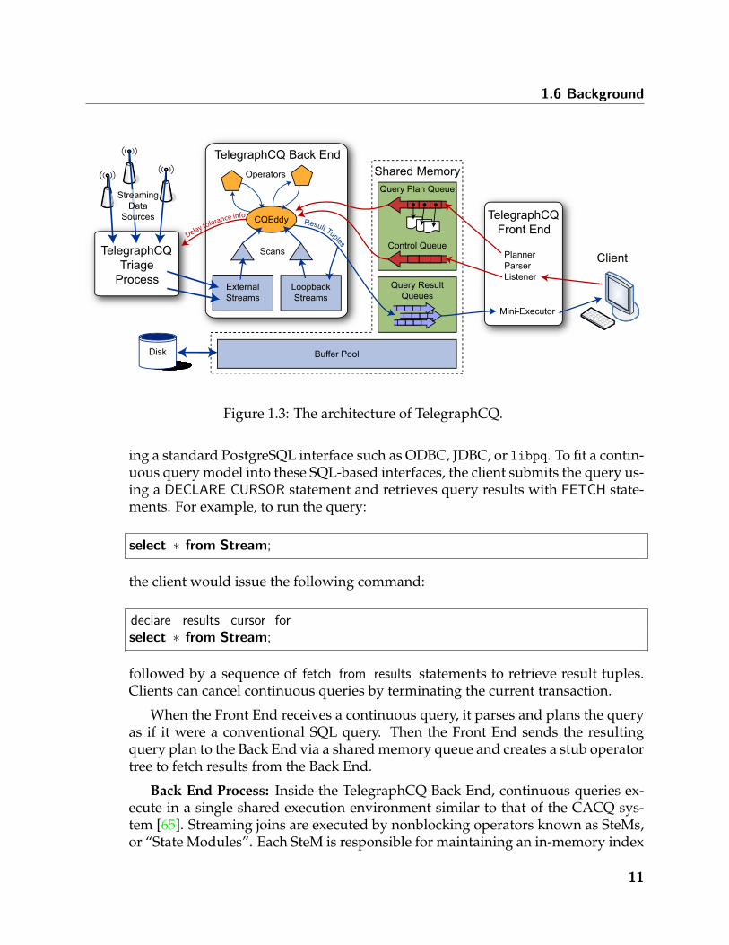
1.6.1.2 Architecture
The architecture of TelegraphCQ version 0.2 was the subject of a CIDR 2003paper [19]. Figure 1.3 shows the architecture of TelegraphCQ version 3.0. Here Ibriefly summarize aspects of the system that are relevant to the understanding ofthis dissertation.
The architecture of TelegraphCQ consists of three major components: The FrontEnd, the Back End, and the Triage Process. Each of these components runs in a sep-arate operating system process; the processes communicate with a combination ofshared memory and Berkeley sockets. The system currently runs on recent Linuxand MacOS platforms.
Front End Process: The TelegraphCQ Front End process has all the componentsof a standard PostgreSQL ”Back End” process; in particular, the TelegraphCQFront End exports the same client APIs as PostgreSQL, and it has full access Tele-graphCQ’s buffer pool and transaction manager. The system spawns a separateFront End process for each client connection, and conventional SQL queries runentirely within the Front End. The Front End forwards CQL continuous queriesto the Back End process and uses a stub “mini-executor” to fetch results from theBack End.
To run a continuous query on TelegraphCQ, clients connect to TelegraphCQ us-
10
1.6 Background
Query Result
Queues
Query Plan Queue
Control Queue
CQEddy
TelegraphCQ Back End
TelegraphCQ
Front End
Shared Memory
External
Streams
Loopback
Streams
Scans
Buffer PoolDisk
Listener
Mini-Executor
Planner
ParserClient
TelegraphCQ
Triage
Process
Delay tolerance info
Streaming
Data
Sources
Operators
Result Tuples
Figure 1.3: The architecture of TelegraphCQ.
ing a standard PostgreSQL interface such as ODBC, JDBC, or libpq. To fit a contin-uous query model into these SQL-based interfaces, the client submits the query us-ing a DECLARE CURSOR statement and retrieves query results with FETCH state-ments. For example, to run the query:
select ∗ from Stream;
the client would issue the following command:
declare results cursor forselect ∗ from Stream;
followed by a sequence of fetch from results statements to retrieve result tuples.Clients can cancel continuous queries by terminating the current transaction.
When the Front End receives a continuous query, it parses and plans the queryas if it were a conventional SQL query. Then the Front End sends the resultingquery plan to the Back End via a shared memory queue and creates a stub operatortree to fetch results from the Back End.
Back End Process: Inside the TelegraphCQ Back End, continuous queries ex-ecute in a single shared execution environment similar to that of the CACQ sys-tem [65]. Streaming joins are executed by nonblocking operators known as SteMs,or “State Modules”. Each SteM is responsible for maintaining an in-memory index
11

Chapter 1: Introduction
of one side of a join. Selections and projections are handled by conventional Post-greSQL operators and a special Grouped Selection Filter operator that can performmultiple selections at once. Aggregation occurs in a special operator that uses treeof PostgreSQL operators to compute aggregate values for each window. Tuplesenter the back end via modified PostgreSQL scan operators. These scans can readtuples from relations, live data streams, or the result streams of existing queries.A special operator known as a CQEddy acts as a nexus of control, coordinatingthe movement of tuples among different relational operators. The CQEddy adap-tively routes tuples among operators, using operator selectivities to determine anefficient execution order.
When a query plan enters the Back End, the CQEddy decomposes it into acollection of operators and merges this collection with the current set of “live”operators, removing duplicates. If multiple queries share a single operator, only asingle instance of the operator is created. Where possible, compatible predicatesare merged into a single Grouped Selection Filter operator. The CQEddy maintainsstate about which queries each tuple satisfies and forwards query results to theFront End as they are produced.
As noted in the previous section, TelegraphCQ supports subqueries and recur-sion via a SQL99-like WITH syntax. Internally, the backend uses “stub” streamsto implement the internal queries of these WITH clauses. Instead of sending theresults of these subqueries to the Front End, the system forwards the result tuplesto scan operators, where the tuples re-enter the CQEddy’s collection of operators.
Triage Process: The Triage Process is the component of TelegraphCQ that pro-vides buffering and latency management for incoming data streams. This com-ponent is the main focus of this dissertation, and subsequent chapters describethe internal structure of the Triage Process in detail. Streaming data sources senddata to the Triage Process, which forwards this data to the Back End as a mixtureof PostgreSQL tuples and compact summaries. The Back End sends informationabout the delay tolerance of queries to the Triage Process, which uses this informa-tion to determine the necessary mix of buffering and summarization. Internally,the Triage Process keeps tuples in their native binary or text format, convertingthem to a format that PostgreSQL (and hence TelegraphCQ) can recognize whensending tuples to the Back End.
12

Chapter 2
Related Work
Everything of importance has been said before by somebody who did not discover it.
— Alfred North Whitehead (1861 - 1947)
13

Chapter 2: Related Work
2.1 IntroductionThis chapter presents a survey of previous work that is relevant to this thesis.
The chapter breaks down this previous work according to which chapter of thethesis is most relevant to it.
2.2 ArchitectureThe problem of monitoring bursty network traffic with inexpensive hardware
has received attention in the networking literature. My solution to this problem,the Data Triage architecture, makes use of with a query processor that is provi-sioned for the data stream’s average data rate. The networking community, incontrast, has taken a different approach to the problem, working to lower the CPUrequirements of query processing itself.
The Gigascope system [25, 24] is one of the more well-known examples of thisapproach. Rather than build a general-purpose query processor, the designers ofGigascope designed a system that is closely tied to a small set of network moni-toring applications. Gigascope operates directly on raw network packets, using aquery language with primitives for composing hard-coded modules. These mod-ules perform the “inner loops” of query processing and are coded in low-levellanguages by experts. Some modules are implemented on special-purpose hard-ware [86]. Because the low-level portions of Gigascope are so specialized andheavily optimized, the system can monitor high-speed network links with rela-tively inexpensive hardware. The major disadvantage of this approach is that itrequires hours of time for experts to implement new queries. My architecture, incontrast, uses a general-purpose streaming query processor, so that relatively un-sophisticated users can write new queries quickly.
The CoMo system [48] represents another approach to keeping hardware costsunder control: Limit the real-time functionality of the system. The streaming com-ponent of CoMo is hard-coded by experts for “line speed” operation, but its func-tionality is limited to maintaining an on-disk circular buffer of recent network traf-fic. Basic query language allows remote sites to extract data from the buffer foroffline analysis with data-mining tools. Compared with my work, CoMo is a muchsimpler architecture to implement, but it provides limited real-time analysis andalert generation.
The SNORT intrusion detection system [92] addresses the hardware cost prob-lem by using a very simple query language. SNORT queries, known as “rules,”can express simple selections and projections over the packet stream. A highlyoptimized execution engine with multi-query optimization takes advantage of thesimplicity of the rules However, complex queries such as joins are difficult or im-
14

2.2 Architecture
possible to express in SNORT’s query language.
The Bro intrusion detection system [30] uses a C-like scripting language for ex-pressing analyses procedurally, with common “inner-loop” operations hard-codedin hand-optimized C++. Sophisticated users can use the scripting language towrite high-level operations, including “contingency plans” for dealing with var-ious overload situations. A combination of hand-optimized low-level code andsophisticated algorithms in the high-level code allows Bro to identify complex pat-terns on relatively inexpensive hardware. However, the use of a procedural lan-guage instead of a declarative one makes modifying Bro’s queries difficult andlimits the ability of unsophisticated users to write new analyses.
2.2.1 Overload Handling
Overload handling is a natural concern in stream query processing, and sev-eral pieces of previous work have proposed solutions to the problem. The Au-rora continuous query system sheds excess load by inserting drop operators intoits dataflow network [104]. My work differs from this approach in two ways: Firstof all, I use fixed end-to-end delay constraints, whereas Aurora’s drop operatorsminimize a local cost function given the resources available. Secondly, my sys-tem adaptively falls back on approximation in overload situations, while Aurorahandles overload by dropping tuples from the dataflow.
Other work has focused on choosing the right tuples to drop in the event ofoverload [27, 53, 100]. My work is complementary to these approaches. In mywork, I do not focus on choosing “victim” tuples in the event of overflow; rather, Idevelop a framework that sends the victim tuples through a fast, approximate datapath to maintain bounded end-to-end latency. Choosing the right victim tuples forData Triage is an important piece of future work.
Other stream processing systems have focused on using purely approximatequery processing as a way of handling high load [15, 60]. Load shedding systemsthat use this approach lossily compress sets of tuples and perform query process-ing on the compressed sets. The STREAM data manager [33] uses either drop-ping or synopses to handle load. In general, this previous work has focused onsituations in which the steady-state workload of the query processor exceeds itscapacity to process input streams; I focus here on provisioning a system to han-dle the steady state well and to degrade gracefully when bursts lead to temporaryoverload.
Techniques for providing fast, approximate answers to queries are awell-studied area in database research. My Data Triage architecture uses theseapproximate query processing techniques as a fall-back mechanism for overloadhandling, and the third part of my proposed thesis presents new techniques for
15

Chapter 2: Related Work
approximating a class of query that is important for network monitoring.
Approaches to approximate query processing generally involve either randomsamples or summary data structures. Random sampling has a long history in theliterature; Olken and Rotem [74] summarize work in the area prior to 1995. Asrecent examples, Chaudhuri et al. [21] analyze the effects of random sampling ofbase relations on the results of joins of those relations. Acharya et al. present atechnique called join synopses that involves sampling from the join of the tablesin a star schema rather than from the base tables themselves [3]. CongressionalSampling [2] and Dynamic Sample Selection [8] collect biased samples to improvethe accuracy of grouped aggregation.
Summary data structures are also well-studied. Garofalakis and Gibbons givea good overview of work in this area [36]. Chakrabarti et al. [17] describe methodsof performing query processing entirely in the wavelet domain using multidimen-sional wavelets. Getoor et al. [38] use probabilistic graph models as a compressedrepresentation of relations. Pavlov, Smith, and Mannila [77, 76] investigate meth-ods for lossy summarization of large, sparse binary data sets. Wang et al. havestudied methods of performing query processing and selectivity estimation usingwavelets [67, 66, 109]. Lim et al. use query feedback to tune a materialized set ofhistograms to the workload of the database [62].
2.3 PolicyChapter 4 of this thesis explains the Delay Constraints API for controlling the
tradeoff between query result latency and accuracy in Data Triage. I develop ascheduling algorithm for the Triage Process that ensures that it meets its con-straints on query result delay. Scheduling algorithms that meet constraints ondelay are common in multimedia scheduling and in real-time systems, but thisprevious work differs from my work in several important respects.
For “hard” real-time applications like avionics and nuclear power plant con-trol, various algorithms can compute processor schedules to ensure that a set ofwell-understood tasks meet a specified set of deadlines with 100 percent proba-bility. The most well-known of these approaches are Rate Monotonic and EarliestDeadline First (also known as Deadline Driven) scheduling, published by Liu andLayland in 1973 [63]. Rate Monotonic scheduling precomputes a static schedule fora fixed set of periodic tasks, guaranteeing that all tasks meet specified deadlines.The Earliest Deadline First approach schedules a stream of incoming tasks, givinghighest priority to Follow-on work has extended these algorithms in a number ofways. For example, the Spring scheduling algorithm adds support for admissioncontrol and distribution and has been implemented in hardware [85, 16]; and Lu et
16

2.3 Policy
al.add closed-loop control to support tasks with unpredictable runtimes [64].
In “soft” real time applications like multimedia scheduling, the scheduler pro-vides probabilistic guarantees that tasks will be finished on time. Lottery schedul-ing [107] and stride scheduling [108] schedule tasks in fixed ratios to ensure thatevery task receives at least the requested amount of CPU time per second. FairQueueing algorithms [72, 28, 9, 97, 102] provide similar guarantees when routingpackets from multiple flows across a network. The Dynamic Window-ConstrainedScheduling algorithm [111] divides network bandwidth between multiple streamswith different “deadlines” (maximum end-to-end latency of any packet) and “loss-tolerances” (percentage of packets in a given period of time that the network isallowed to drop).
In my work, I study a significantly different scheduling problem than previ-ous work in real-time systems and networking. Existing work on processor andnetwork scheduling focuses on determining the correct order in which to performa collection of different tasks in order to ensure that all the tasks meet individualdeadlines with high probability. The Data Triage scheduling problem, in contrast,involves scheduling the processing of a stream of very small, substantially identi-cal tuple processing tasks, with every tuple from a given window having the samedeadline. Since the tuples in a streaming query processor must be processed in or-der, the individual tasks in Data Triage occur in a very constrained order; choosingan order of operations is not an important factor in my work. The chief decisionthat my scheduling algorithm must make is whether to triage or to process fullythe tuple currently at the head of the Triage Queue.
17

Chapter 2: Related Work
2.4 HistogramsChapter 5 of this thesis describes a new class of histogram that I have de-
veloped. Histograms have a long history in the database literature. In recentyears, researchers have developed many heuristics for constructing histograms[82, 69, 51, 12, 29, 103]. Other work has focused on optimal algorithms for his-togram construction [49, 50, 51]. Poosala et al.[81] give a good overview of work inone-dimensional histograms, and Bruno et al.[12] provide an overview of existingwork in multidimensional histograms.
Previous work has identified histogram construction problems for queries overhierarchies in data warehousing applications, where histogram buckets can be ar-bitrary contiguous ranges. Koudas et al.first presented the problem and providedan O(n6) solution [57]. Guha et al.developed an algorithm that obtains “near-linear” running time but requires more histogram buckets than the optimal so-lution [44]. Both papers focus only on Root-Mean-Squared (RMS) error metrics. Inmy work, I consider a different version of the problem in which the histogrambuckets consist of nodes in the hierarchy, instead of being arbitrary ranges; andthe selection ranges form a partition of the space. This restriction allows us todevise efficient optimal algorithms that extend to multiple dimensions and allownested histogram buckets. Also, I support a wide variety of error metrics.
The STHoles work of Bruno et al.introduced the idea of nested histogram buck-ets [12]. The “holes” in STHoles histograms create a structure that is similar to mylongest-prefix-match histogram buckets. However, I present efficient and optimalalgorithms to build my histograms, whereas Bruno et al.used only heuristics (basedon query feedback) for histogram construction. My algorithms take advantage ofhierarchies of identifiers, whereas the STHoles work assumed no hierarchy.
Bu et al.study the problem of describing 1-0 matrices using hierarchical Mini-mum Description Length summaries with special “holes” to handle outliers [13].This hierarchical MDL data structure has a similar flavor to the longest-prefix-match partitioning functions I study, but there are several important distinctions.First of all, the MDL summaries construct an exact compressed version of binarydata, while my partitioning functions are used to find an approximate answerover integer-valued data. Furthermore, the “holes” that Bu et al.study are strictlylocated in the leaf nodes of the MDL hierarchy, whereas my hierarchies involvenested “holes”.
Wavelet-based histograms [67, 66] are another area of related work. The errortree in a wavelet decomposition is analogous to the UID hierarchies I study. Also,recent work has studied building wavelet-based histograms for distributive errormetrics [37, 54]. My overlapping histograms are somewhat reminiscent of wavelet-based histograms, but my concept of a bucket (and its contribution to the his-
18

2.5 Deployment
togramming error) is simpler than that of a Haar wavelet coefficient. This resultsin simpler and more efficient algorithms (in the case of non-RMS error metrics),especially for multi-dimensional data sets [37]. In addition, my histogrammingalgorithms can work over arbitrary hierarchies rather than assuming the fixed, bi-nary hierarchical construction employed by the Haar wavelet basis.
My longest-prefix-match class of functions is based on the technique usedto map network addresses to destinations in Internet routers [35]. Networkingresearchers have developed highly efficient hardware and software methods forcomputing longest-prefix-match functions over IP addresses [73] and generalstrings [14].
2.5 DeploymentTwo previous studies have used TelegraphCQ to run simple network monitor-
ing queries [80, 87]. In the deployment study I describe in Chapter 6, I embedTelegraphCQ in an end-to-end system and use a larger workload of more complexqueries to get a more realistic view of TelegraphCQ’s performance.
The objective of the work presented in [22] is to build a database system foranalyzing off-line network traffic data for studying coordinated scan activities.Another recent database effort for analyzing network traffic is described in [98].Both approaches use open source database systems and index data structures forefficient analysis of off-line network traffic data. However, these systems do notmanage streaming data.
A combination of live and historic data processing is presented in [20]. Historicdata is managed by a B-tree that is adaptively updated based on the query load. Inorder to keep up with high query loads, the B-tree updates are delayed for periodswith lower traffic. Thus, historic queries can operate on reduced (sampled) datasets during high loads. This leads to approximate answers for queries on historicaldata, which may affect analysis results. Rather than B-trees, we use bitmap indicesfor querying historic data. One reason for this change is that the bitmap indicescan answer multi-dimensional range queries quickly and accurately [75, 18, 114,93, 115]. Such queries appear frequently in my network monitoring workload.
One of the motivations given in [20] for their work was that updating B-treesmay take too much time to keep up with the arrival of new records. In my work,I reexamine this assumption in the context of bitmap indices and show that indexinsertions do not need to be a bottleneck. Unlike B-trees, bitmap indices do notrequire sorting of the input data. This property allows for very efficient bulk ap-pend operations. Recent proposals for improving the write performance of B-Trees[40] may narrow this performance gap, but I am unaware of any hard performance
19

Chapter 2: Related Work
numbers for the new designs.
In the network community, two commonly used Intrusion Detection Systemsare Bro [78] and Snort [91]. These systems are used to analyze and react to suspi-cious or malicious network activity in real time. Recently Bro was extended by aconcept called the time machine [56], i.e. to analyze historic data by traveling backin time. The high-level concept of a time machine is similar to the one described inChatper 6. However, the authors do not provide any details on the performance ofquerying historic data. The goal of my study is to provide a detailed performanceanalysis on the combination of stream processing and historic data analysis. In ad-dition, the analyses in Bro and Snort are performed through C-like scripting lan-guage with manual management of data structures, while the system described inChapter 6 uses high-level declarative queries. In contrast, similar scripts writtenin declarative languages such as SQL are much more compact and much easier tocreate.
FastBit implements a set of compressed bitmap indices using an efficient com-pression method called the Word Aligned Hybrid (WAH) code [114, 115]. In an num-ber of performance measurements, WAH compressed indices were shown to sig-nificantly outperform other indices [113, 114]. Recently, FastBit has also been usedin analysis of network traffic data and shown to be able to handle massive datasets [101, 11]. This earlier proof-of-concept made FastBit a convenient choice forthe prototype described in Chapter 6.
20

Chapter 3
Architecture
21

Chapter 3: Architecture
3.1 IntroductionThis chapter describes the Data Triage architecture and its implementation in theTelegraphCQ streaming query processor. Data Triage provides a software fallbackmechanism to isolate the query processor from high-speed bursts. The architectureshunts excess data through a shadow query that uses approximation to summarizemissing query results.
The chapter starts with a brief overview of approximate query processing, fol-lowed by a description of the architecture. Then I describe techniques for imple-menting approximate query processing in a general-purpose query processor likeTelegraphCQ. Finally, I describe the query rewrite process that my system uses toproduce shadow queries.
3.1.1 Approximate Query Processing with Summaries
Much work has been done on approximate relational query processing usinglossy set summaries. Originally intended for query optimization and interactivedata analysis, these techniques have also shown promise as a fast and approximatemethod of stream query processing. Examples of summary schemes include ran-dom sampling [106, 3], multidimensional histograms [82, 51, 29, 103], and wavelet-based histograms [17, 67].
Later in this dissertation, in Chapter 5, I will present my work in approximat-ing an important class of queries in the network monitoring space. However, thework in the current chapter centers on leveraging any kind of query approxima-tion, including my histograms and the broad body of previous work. No singlesummarization method has been shown to dominate all others for all query types,so my system supports a variety of techniques. To simplify this support, I have de-veloped a generic framework that allows my system to implement most existingapproximations.
My framework divides an approximation scheme into four components:
• A summary data structure that provides a compact, lossy representation of a setof relational tuples
• A compression function that constructs summaries from sets of tuples.
• A set of operators that compute relational algebra expressions in the summarydomain.
• A rendering function that converts from the summary domain back to the rela-tional domain by generating tuples containing either aggregates over the inputstream or representatives of that stream.
22

3.2 Data Triage
Tri
ag
e L
ayer
Qu
ery
En
gin
e
Initial Filteringand Parsing
The shadow
query computes
approximately
what results are
missing from the
main query
Shadow
Query
Summaries of
Sets of Tuples
The main portion of
the query operates
without regard to
load-shedding.
Main Query
TriagedTuples
Merge
Results
Summarizer
TriageScheduler
Triage
Queue
Summaries of
Missing Results
RawPackets
Render
Results
Figure 3.1: An overview of the Data Triage architecture. Data Triage acts as a middlewarelayer within the network monitor, isolating the real-time components from the best-effortquery processor to maintain end-to-end responsiveness.
These primitives allow one to approximate continuous queries of the type de-scribed in Section 1.6.1.1. First, summarize the tuples in the current time window,then run these summaries through a tree of operators, and finally render the ap-proximate result.
In addition to the primitives listed above, each approximation technique alsohas one or more tuning parameters. Examples of such parameters include samplerate, histogram bucket width, and number of wavelet coefficients. The tuning pa-rameters control the tradeoff between processing time and approximation error.
3.2 Data TriageFigure 3.1 gives an overview of the Data Triage architecture. This architectureconsists of several components:
• The initial parsing and filtering layer of the system decodes network packets orflow records and produces streams of binary data tuples containing detailed
23

Chapter 3: Architecture
information about the packet stream.
• The Main Query operates inside a stream query processor; my prototype usesthe TelegraphCQ query processor. The query processor converts tuples fromthe initial parsing and filtering layer into its internal format and passes themthrough the Main Query. Architecturally, the key characteristic of this query isthat it is tuned to operate at the network’s typical data rate. Data Triage protectsthe main query from data rates that exceed its capacity.
• A Triage Queue sits between each stream of tuples and the main query. TriageQueues act as buffers to smooth out small bursts, and they provide a mecha-nism for shunting excess data to a software fallback mechanism when there isnot enough time to perform full query processing on every tuple.
• The Triage Scheduler manages the Triage Queues to ensure that the system deliv-ers query results on time. The Scheduler manages end-to-end delay by triagingexcess tuples from the Triage Queues, sending these tuples through the ShadowQuery. I give a detailed description of my scheduling algorithm in Section 4.4.
• The Summarizer builds summary data structures containing information aboutthe tuples that the Scheduler has triaged. The Summarizer then encapsulatesthese summaries and sends them to the query engine for approximate queryprocessing.
• The Shadow Query uses approximate query processing over summary datastructures to compute the results that are missing from the main query. Theouter clause of his query then renders the summary into a set of relationaltuples that represents the approximate result.
• The Merge Query merges the results of the Main and Shadow queries to producea unified query answer for each time window. For GROUP BY queries, thismerge involves a join on the grouping columns. For queries that produce a setof base tuples, the merge involves a UNION ALL clause.
I have implemented Data Triage in the TelegraphCQ stream query processor.The sections that follow describe the approach I used to construct approximateshadow queries efficiently.
3.2.1 Approximate Query Processing Framework
An important challenge of implementing Data Triage is adding the approxi-mate query processing components to the query engine without rearchitecting thesystem. As I noted earlier in this chapter, most query approximation techniquescan be divided into four components: a summary data structure, a compressionfunction, a set of operators, and a rendering function. To perform approximate
24

3.2 Data Triage
query processing in TelegraphCQ, I have mapped these four components ontoTelegraphCQ’s object-relational capabilities. This implementation permits the useof many different summary types and minimizes changes to the TelegraphCQquery engine.
At the core of an approximation scheme is the summarization data structure,which provides a compact, lossy representation of a set of relational tuples. Iused the user-defined datatype functionality of TelegraphCQ to implement sev-eral types of summary data structures, including reservoir samples, two types ofmultidimensional histograms, and wavelet-based histograms.
The second component of a summary scheme is a compression function for sum-marizing sets of tuples. My implementation actually divides the compression func-tion into three parts, a design similar to the user-defined aggregates in PostgreSQL.The first part of a compression is a routine for creating an empty summary; the sec-ond part is a routine for adding a tuple to an existing summary; and the third partis a routine that finalizes the summary and prepares it to be sent to TelegraphCQ.
The Summarizer takes a compression function as an argument, with differ-ent C++ classes implementing different summarization schemes. This summaryis packed into the external representation (currently text) of a user-defined typeand sent to TelegraphCQ as a field of a tuple. The constructor for the user-definedtype converts this external representation into an internal binary representation ofthe summary. In my experiments, the overhead of this conversion represented avery small part of overall running time. If necessary, a production implementa-tion of the Summarizer could avoid this conversion step entirely by generating theinternal binary representation of the summary directly.
The third component of a summary scheme is a set of relational operatorsthat operate on the summary domain. Once summaries are stored in objects, itis straightforward to implement relational operators as functions on these objects.In TelegraphCQ, the syntax to define user-defined function over a user-definedtype is derived from that of PostgreSQL:
CREATE FUNCTION function name(argument list)RETURNS return type AS’<path to shared object>’, ’<function name>’LANGUAGE C;
where function name is a name used for calling the function from within CQLqueries, return type is the built-in or user-defined type that the function returns,and the shared object and function name tell TelegraphCQ where to find the
25

Chapter 3: Architecture
function implementation at runtime.
If, for example, MHIST multidimensional histograms [82] are encapsulated in auser-defined type, the common relational operators on this type are easily declaredin TelegraphCQ syntax:
−− Project S down to the indicated columns.create function project (S MHIST, colnames cstring)
returns MHIST as ...
−− Approximate SQL’s UNION ALL construct.create function union all (S MHIST, T MHIST)
returns MHIST as ...
−− Compute approximate equijoin of S and T.create function equijoin ( S MHIST, S colname cstring,
T MHIST, T colname cstring)returns MHIST as ...
The C implementation of each function performs the appropriate operations onthe binary representation of the summary. The binary representation of the sum-mary also tracks the mapping between dimensions of a multidimensional sum-mary and the columns of stream tuples. Shadow queries can use calls to thesefunctions to compute relational expressions; for example:
(select b,c from A) UNION ALL (select d,e from B)
becomes
select union all ( project (A.sum, ’b,c’ ), project (B.sum, ’d,e’ )) from A, B;
The final component of a summary scheme is a rendering function that com-putes aggregate values from a summary. TelegraphCQ contains functionality fromPostgreSQL for constructing functions that return sets of tuples. I use this set-returning function framework to implement the rendering functions for the differ-ent datatypes:
−− Convert S into tuples, one tuple for each bucketcreate function mhist render(S MHIST)
returns setof record as ...
26

3.3 Lifetime of a Query
select hist_to_count( hist_project( hist_bandjoin( (select summary from CachedHist where entryname = ‘Whois’), TP.summary, ‘Packets.src_addr’, ‘Whois.min_addr’, ‘Whois.max_addr’ ), ‘Packets.src_addr’ ) ) as shadow, TP.end_ts as tsFrom __triaged_Packets TP;
Shadow Query
insert into CachedHistsselect ‘Whois’, hist_from_query( ‘select min_addr, max_addr from Whois where name like \’%berkeley.edu\’’);
Precompute Static PortionsOriginal QueryOriginal Queryselect count(*), tsfrom Packets P [range ’5 seconds’ slide ’5 seconds’], Whois Wwhere P.src_addr >= W.min_addr and P.src_addr < W.max_addr and W.name LIKE ’%berkeley.edu’limit delay to ’1 second’;
DifferentialRelational Algebra
Final QueryMain Query
ShadowQuery
Packets-Packets+
Packetsnoisy
Whois-Whois+
Whoisnoisy
MergeQuery
with(select count(*)...) as main_q,(select hist_to_count(...)) as shadow_q,(select M.count as main_count, S.count as shadow_count, M.ts as ts from main_q M [range ‘5 seconds’], full outer join shadow_q S [range ‘5 seconds’] where M.ts = S.ts);
Figure 3.2: An illustration of the Data Triage query rewrite algorithm as applied to anexample query. The algorithm produces a main query, a shadow query, and auxiliaryglue queries to merge their results. This example uses multidimensional histograms as asummary datatype.
Having implemented the components of a given summarization scheme, I canconstruct Data Triage’s shadow queries and merging logic using query rewriting.Section 3.3 demonstrates this process on a simple example query.
3.3 Lifetime of a QueryTo illustrate the methods I use to construct shadow queries and how these methodsinteract with my implementation of Data Triage, I will now describe the queryrewrite and execution process as it applies to the query in Figure 4.2. The queryreports the number of packets coming from Berkeley domains every 5 seconds.
3.3.1 Summary Streams
Recall the sample CQL schema from Section 1.6.1.1. This schema contains atable of WHOIS information and a stream, Packet, of information about networkpackets.
To use Data Triage in TelegraphCQ, the user adds an ON OVERLOAD clause toeach CREATE STREAM statement:
27

Chapter 3: Architecture
create stream Packets ...on overload keep MHIST;
This clause specifies the type of summary that Data Triage will construct on excesstuples in the stream. An alternate syntax could have the user choose the sum-mary type at query execution time, though I did not expose such a syntax in myimplementation.
The ON OVERLOAD clause causes TelegraphCQ to generate an auxiliary sum-mary stream for summaries of triaged tuples:
create streamtriaged Packets (summary MHIST,
earliest timestamp,latest timestamp);
The two Timestamp fields in this stream indicate the range of timestamps in thetuples represented by the summary field. The summary stream will serve as aninput to all shadow queries that operate on the Packets stream.
TelegraphCQ supports stream-stream join queries, such as:
select ∗from S [range ’10 sec’ slide ’10 sec’ ],
T [range ’10 sec’ slide ’10 sec’ ]where S.a = T.a;
A more complex example of such a query is my “dispersion” query in Chap-ter 6. As the derivation in Section 3.3.2 indicates, the shadow query for a stream-stream join requires joining the triaged tuples for each stream the non-triaged tu-ples from the other stream. The system could join the summaries directly with thenon-triaged tuples, but it is generally more efficient to summarize these tuples andthen perform the join. To cover the case when a stream-stream join query operatesdirectly on base streams, my system also creates a second summary stream thatsummarizes non-triaged tuples:
create streamnontriaged Packets (summary MHIST,
earliest timestamp,latest timestamp);
28

3.3 Lifetime of a Query
This second stream and its associated summarizer are only activated when astream-stream joins query is present in the system.
3.3.2 Query Rewrite
Figure 3.2 shows the query rewrite process as applied to my sample query. Myquery rewriting methodology is based on an algebraic formalism that allows mysystem to correctly rewrite queries into shadow queries. I use relational algebrato build a set of differential relational algebra operators. My approach here resemblespast work in maintaining materialized views [45], though my setting is different.
Each differential operator propagates changes from the inputs to the outputsof the corresponding relational algebra operator. In naming the components of thealgebra, I borrow a convention from the field of signal processing. When analyzinga noisy analog channel, it is a common practice to break the channel into “signal”and “noise” components and to model these components separately. Similarly, thedifferential relational algebra divides each input relation S into noisy, additive noise,and subtractive noise components Snoisy, S+ and S−, such that:
Snoisy ≡ S + S+ − S− (3.1)
where + and − are the multiset union and multiset difference operators, respec-tively. Each differential operator propagates changes to these components sepa-rately.
Note that relational operations like negation and set difference can cause addi-tional tuples to appear in an expression’s output when tuples are removed fromits inputs. The additive noise component in the differential relational algebra com-pensates for these additional tuples. For base relations and subexpressions thatdo not contain negation or set difference operators, the additive noise componentof the shadow query is always empty. In general, the empty parts of a rewrittenshadow query can be pruned by substituting the empty set (∅) for these parts andsimplifying the resultant relational algebra expression. Appendix A gives detaileddefinitions of several important differential operators, including the set differenceoperator.
My query rewriter starts by constructing a differential relational algebra ex-pression for each SELECT clause in the original query. Each differential operator isdefined in terms of the basic relational operators. The query rewriter recursivelyapplies these definitions to the differential relational algebra expression to obtain arelational algebra expression for the tuples that are missing from the main query’soutput. Then the query rewriter removes empty relations and translates the rela-tional algebra expression into the object-relational framework described in Section
29

Chapter 3: Architecture
3.2.1 to produce the shadow query.
Certain portions of the shadow query reference static tables that do not changeduring the lifetime of the user’s continuous query. The query rewriter precom-putes these expressions and stores the resulting summary objects in a system table.At runtime, the shadow query fetches these cached summaries instead of recom-puting the corresponding subexpressions.
Finally, the query rewriter generates a single WITH statement that will run themain and shadow queries and merge their results. The application or GUI frontend submits this rewritten query to the query engine, which begins executing themain and shadow queries.
3.3.3 Query Execution
When TelegraphCQ receives the rewritten query, it passes query parametersto the Triage Process and begins pulling a mix of full tuples and summaries fromthe Triage Queue and Summarizer. The Scheduler monitors the Triage Queue onthe Packets stream and summarizes tuples that the system does not have timeto process fully. Once per time window, the Scheduler sends a summary to the__triaged_Packets stream that serves as an input to the shadow query. TheScheduler throttles the flow of full tuples until the query engine has consumedthe current summary.
The original query returns a single count of packets per time window. In placeof this single count, the rewritten query will instead return two counts per timewindow — one from the main query and one from the shadow query. The ap-plication can add these two counts to obtain an estimate of the true query resultsfor presentation via the appropriate interface. Keeping the results of the main andshadow queries separate provides feedback as to how much approximation wentinto the overall result.
In some applications, it is useful for the shadow query to return error estimatesor confidence intervals, in addition to the counts, aggregate values, or tuples thatthe queries normally produce. For example, the designers of a graphical visualiza-tion may wish to add error bars to indicate a 90% confidence interval. For randomsamples, a set of recursive formulas exist for computing the error in estimating theresults of a relational query with aggregation [46] Most other types of approxima-tion can produce similar, albeit looser, bounds on error.
30

3.4 Extending Data Triage for Archived Streams
Tria
ge
La
ye
r
Initial Filteringand Parsing
Summaries of
Sets of Tuples
TriagedTuples
SummarizerTriage
Queue
RawPackets
Triage
Scheduler
Staging
Area
Query Engine
Index
Bulk
Loader
Fetch
Historical Data
Figure 3.3: Illustration of how Data Triage can be extended to handle archived streams.
3.4 Extending Data Triage for Archived StreamsThe Data Triage architecture as presented in this chapter provides an overloadhandling mechanism for query processors that answer queries over live streams.In many network monitoring applications, it is useful to maintain an archive ofstreaming data from the past. Administrators often need to examine past historyto trace back the source of a problem that a “live” monitoring system detects. Also,historical data can provide a baseline for comparison against current network be-havior, helping to eliminate false positives.
Data Triage can be extended in a straightforward way to handle applicationsthat require keeping an archive of historical streaming data. Figure 3.3 illustrateshow this extension of the architecture works. Archived stream data is stored inan on-disk index. In addition to being sent to the Triage Queue, streaming datais also written to an on-disk staging area. During periods of low system load, abackground process bulk-loads data from the staging area into the index.
This design is partially based on Sirish Chandrasekaran’s work on“live/archive” query processing [20]. Unlike this previous work, my designtakes advantages of “economies of scale” by bulk-loading indexes. My approach
31

Chapter 3: Architecture
leads to a simplified design and higher indexing throughput at the expense ofsomewhat delayed index generation. In Chapter 6, I present an implementationof this design as well as experiments that characterize its throughput benefits andindex loading delays.
32

Chapter 4
Policy
I love deadlines. I like the whooshing sound they make as they fly by.
— Douglas Adams
33

Chapter 4: Policy
4.1 IntroductionThe Data Triage architecture creates a tradeoff between the latency and the accu-racy of query results. Different applications fit at different points along this trade-off. This chapter presents the delay constraints API that I have developed to controllatency and accuracy in Data Triage, along with my techniques for meeting theconstraints this API imposes.
The chapter starts by analyzing the latency-accuracy tradeoff in detail. Then itpresents the API, followed by my scheduling algorithm for implementing this API.I then analyze the problem of provisioning a system with Data Triage, paying par-ticular attention to the performance the system requires from it approximate queryprocessing implementation. I describe the results of a microbenchmark study thatshows that my current implementations of several approximation schemes per-form sufficiently well to provide an order of magnitude of additional data process-ing capacity to TelegraphCQ. Finally, I present an end-to-end experimental studyon my full implementation of Data Triage.
4.2 The Latency-Accuracy TradeoffThe Data Triage architecture uses a combination of buffering and approxima-
tion to handle overload. If tuples enter the Triage Process faster than the mainquery can consume them, the Triage Scheduler has two choices: buffer the excesstuples in the Triage Queue; or triage tuples in the Queue, adding them to the cur-rent approximate summary. Each of these choices has significant ramifications forthe latency and accuracy of the streaming query results that the user sees, as thebenchmarks in the following paragraphs demonstrate. Choosing the right mix ofbuffering and approximation is crucial to maintaining acceptable application per-formance with Data Triage.
Figure 4.1 shows the results of an experiment to measure the latency of queryresults in TelegraphCQ when the system uses buffering to absorb excess data. Thedata source for this experiment was a packet trace from the Lawrence BerkeleyNational Laboratories web server. I played back this trace through TelegraphCQ,using a schema similar to that in Section 1.6.1.1. I configured TelegraphCQ to runthe query:
select count(∗) from Packets [range ’10 sec’ slide ’10 sec’ ];
My software used the timestamps in the trace to determine when to send tuplesto TelegraphCQ. To simulate a less-powerful machine, I increased the playbackrate of the trace by a factor of 10 and reduced the query window by a factor of 10.At these settings, the query processor was provisioned for the 90th percentile of
34

4.2 The Latency-Accuracy Tradeoff
0 100 200 300 400 500012345678
Offset into Trace (sec)
Que
ry R
esul
t Lat
ency
(sec
)
Figure 4.1: Query result latency for a simple aggregation query over a 10-second timewindow. The query processor is provisioned for the 90th percentile of packet arrivalrates. Data is a trace of a web server’s network traffic.
packet arrival rates. The graph shows the observed latency between query resultgeneration and the end of each time window.
About 200 seconds into the trace, a burst of high-speed data overwhelms thecapacity of the main query to consume data. As the amount of data in the TriageQueue increases, the buffering creates a rapidly-increasing delay between data ar-rival and query result generation. When the burst ends, this high latency persistsfor several time windows as the query processor gradually drains the buffer. Notethat the heavy-tailed distribution of burst lengths means that this latency is poten-tially unbounded in practice.
Of course, the Triage Scheduler can limit query result latency by triaging tuples,removing them from the Triage Queue and incorporating them into a compressedsummary. As long as there is enough time to summarize the entire input stream,the Scheduler can impose arbitrary limits on query result latency by limiting thenumber of tuples in the Triage Queue. However, this latency reduction comesat a significant cost: As the system triages larger fractions of the input data, theaccuracy of query results will necessarily go down.
The Triage Scheduler must choose the right mix of buffering and approxima-tion to ensure that the system meets application requirements for latency and ac-curacy. Unfortunately, different network monitoring applications have vastly dif-
35

Chapter 4: Policy
select count(∗)from Packets P [range by ’5 seconds’ slide by ’5 seconds’ ], Whois Wwhere P.src\string addr ≥W.min\string addr
and P.src\ string addr < W.max\string addrand W.name LIKE ’\%berkeley.edu’
limit delay to ’1 second’ ;
Figure 4.2: Sample query with a delay constraint
ferent requirements for these two metrics. For example, systems that detect andrespond to security breaches [110] require very low latency but can tolerate falsepositives. At the other extreme, systems that produce digests of network traffic be-havior for offline analysis can tolerate several hours of delay but need to producedetailed, accurate results.
In the applications that I have studied, latency requirements are more strictand show significantly more variation across applications, compared with require-ments for result accuracy. Because of this asymmetry, my research has focusedon maintaining strict limits on query result latency while delivering the most ac-curate query results possible. In the sections that follow, I propose an API calleddelay constraints that allows applications to inform the Triage Scheduler of their tol-erance for query result latency on a per-query basis. Later in the chapter, I presenta scheduling algorithm that allows the Triage Scheduler to meet a delay constraintwhile minimizing the system’s reliance on approximation.
4.3 Delay ConstraintsA delay constraint is a user-defined bound on the latency between data arrival
and query result generation. Figure 4.2 shows an example of my syntax for delayconstraints. My modification to CQL adds the optional clause
limit delay to [ interval ]
to the end of the SELECT statement.
If the SELECT clause does not involve windowed aggregation, the delay con-straint bounds the delay between the arrival of a tuple and the production of itscorresponding join results. When the SELECT clause contains a windowed ag-gregate, the delay constraint becomes what I call a windowed delay constraint. Awindowed delay constraint of D seconds means that the aggregate results for atime window are available at most D seconds after then end of the window.
Most of the monitoring queries I have studied contain windowed GROUP BY
36

4.3 Delay Constraints
Variable Units Description
D sec The delay constraintW sec Size of the query’s hopping windowC f ull sec (CPU) Incremental CPU cost of sending a tuple through the main
query in Data TriageCshadow sec (CPU) Cost of sending a tuple through the shadow queryCtup sec (CPU) Overall cost of processing a tupleCsum sec (CPU) CPU cost of adding a tuple to a summaryRpeak
tuplessec The highest data rate that Data Triage can handle
Rexacttuples
sec The highest data rate at which Data Triage does not useapproximation
Table 4.1: Variables used in Sections 4.4 through 4.7
and aggregation, so I concentrate here on delay constraints for windowed queries.
Table 4.1 summarizes the variable names used in this section and the ones thatfollow. Consider a query with a hopping time window of size W and a windoweddelay constraint of D seconds. Let wt denote the time window to which a giventuple t belongs, and let Ctup denote the marginal cost of processing a tuple. Weassume that Ctup is constant across all tuples; I discuss relaxing this assumption inthe Future Work section. Let end(w) denote the end of window w.
The delay constraint defines a delivery deadline for each tuple t of
deadline(t) = end(wt) + D − Ctup (4.1)
It can be easily shown that, if the query processor consumes every tuple before itsdelivery deadline, then the query engine satisfies the delay constraint.
Note that every tuple in a hopping window has the same deadline. Duringthe remainder of this chapter, I denote the deadline for the tuples in window w bydeadline(w)
37

Chapter 4: Policy
4.4 The Triage SchedulerThe Triage Scheduler is the control component of Data Triage. The Scheduler’sprimary purpose is to ensure that the system meets the current delay constraint.The Triage Scheduler meets this goal by controlling three important decisions:
• Whether to send a tuple from the Triage Queue to the main query
• Whether to “triage” a tuple from the Triage Queue, by adding it to a summary
• Whether to transfer the current summary from the Summarizer to the shadowquery.
Sending tuples to the summarizer supports significantly higher data rates thanfull query processing, but compression operations do not have nonzero cost. AsI will show in my experiments, summarizing a large number of triaged tuplesrequires a relatively small but still significant amount of CPU time. Likewise, rela-tional operations on summaries can take a significant amount of time, though theyonly occur once per time window. In order to satisfy the user’s delay constraints,the Triage Scheduler needs to take these costs into account when deciding whichtuples to triage and when to triage them.
Recall from the previous section that a delay constraint of D defines a tupledelivery deadline of deadline(t) = end(wt) + D − Ctup for each tuple t, whereCtup is the time required to process the tuple.
In the Data Triage architecture, the value of Ctup depends on which datapatha tuple follows. Let C f ull denote the CPU time required to send a tuple throughthe main query, and let Csum denote the CPU time to add a tuple to the current
summary. Then: Ctup =
C f ull (for main query)Csum (for shadow query)
The Triage Scheduler also needs to account for the cost of sending summariesthrough the shadow query. Let Cshadow denote the cost per time window of theshadow query, including the cost of merging query results. I assume that Cshadow isconstant regardless of the number of tuples triaged. I assume that the system usesa single CPU. Under this assumption, an increase in Cshadow decreases the amountof processing time available for other operations.
Incorporating the costs of the approximate datapath into the deadline equationfrom Section 4.3, I obtain the new equation:
deadline(w) = end(w) + D − Cshadow −
C f ull (for main query)Csum (for shadow query)
(4.2)
38

4.4 The Triage Scheduler
In other words, the deadline for a tuple depends on whether the tuple is triaged.Of course, whether the tuple is triaged depends on the tuple’s deadline.
One can satisfy all the above requirements with a single scheduling invariant.Intuitively:
Time to process remainingtuples in window ≤ Time before delay
constraint violated. (4.3)
More formally, letting n denote the number of tuples in the Triage Queue, Wthe window size, O the real-time offset into the current window, and C f ull the costof sending a tuple through the main query:
nC f ull ≤ W + D − Cshadow − O, (4.4)
or equivalently
n ≤(
W + D − CshadowC f ull
)− O
C f ull. (4.5)
As long as the Triage Scheduler maintains this invariant (by triaging enoughtuples to keep n sufficiently low), the query processor will satisfy its delay con-straint. I note that the Scheduler must maintain the invariant simultaneously forall windows whose tuples could be in the Triage Queue.
It is important to note that n, the number of tuples that can reside in the TriageQueue without violating this invariant, decreases linearly throughout each time win-dow. One could imagine using a fixed queue length to satisfy the invariant, butdoing so would require a queue length of the minimum value of n over the entirewindow. In other words, using a fixed-length queue causes the system to triagetuples unnecessarily. In keeping with my philosophy of using approximation as afallback mechanism, my scheduler avoids triaging tuples for as long as possible bycontinuously varying the number of tuples from the window that are permitted toreside in the Triage Queue. Figure 4.3 illustrates this variation in effective queuelength.
39

Chapter 4: Policy
Offset into Window (sec)
Effe
ctiv
e Q
ueue
Len
gth
WCshadow
D
0 1 2 3 4 5 6 70
1000
2000
3000
4000
5000
6000 Next window
Effective queue length for this window
Figure 4.3: The effective length of the Triage Queue for tuples belonging to a 5-secondtime window, as a function of offset into the window. The delay constraint is 2 seconds,and Cshadow is 1 second.
4.5 General Sliding WindowsThe previous sections have described my implementation of the Triage Scheduleras it applies to nonoverlapping, or “hopping,” time windows. Extending this workto multiple queries with general sliding windows is straightforward.
Briefly, the framework described in this chapter can accommodate arbitrarycombinations of TelegraphCQ window clauses with the following changes:
• Use the method described in [58] to convert overlapping time windows to arepeating sequence of nonoverlapping windows.
• Compute delay constraints for each of the nonoverlapping windows by deter-mining the query delay constraints that apply at a given point in the sequence.
• When constructing shadow queries, use user-defined aggregates to merge sum-maries from adjacent windows as needed.
In the remainder of this section, I explain these steps in greater detail.
4.5.1 Converting overlapping windows
The main challenge in supporting general sliding windows is that the windowscan overlap. In particular, a tuple could belong to any number of time windows.
40

4.5 General Sliding Windows
If a tuple can be a member of n windows, the system should to avoid adding thetuple to n summaries.
Krishnamurthy et al. have developed a general method of converting any com-bination of overlapping window specifications into a sequence of nonoverlappingtime windows [58]. The idea behind this approach is to create a new nonoverlap-ping window whenever one of the overlapping windows advances. The transfor-mation produces a repeating sequence of overlapping windows of varying widths.The Triage Scheduler produces a summary for each of these nonoverlapping win-dows.
4.5.2 Computing delay constraints
Once the original set of sliding windows has been converted into a sequence ofnonoverlapping windows, the system assigns a separate delay constraint to eachwindow in the sequence. To compute the delay constraint for a given nonover-lapping window, the system starts by computing the result delivery deadline forevery sliding window that contains the nonoverlapping window. The delay con-straint is set to the time from the end of the nonoverlapping window to the earliestsuch deadline.
This approach guarantees that the Triage Scheduler will not triage a tuple un-less at least one query requires triage in order to meet its delay constraint. At thesame time, the approach is somewhat conservative in that not every query mayrequire that a given tuple be triaged. If there is a large difference in delay toleranceamong queries, the system can divide the queries into clusters and create multiple“copies” of the input stream, one for each cluster. This approach is similar to theclustering technique used by Krishnamurthy et al.[59].
4.5.3 Using aggregates to merge summaries
Once the system has converted a sliding window to a set of nonoverlappingwindows, it needs an efficient way to merge sets of adjacent nonoverlapping win-dows into a single sliding window. To perform this merging, I create a user-defined aggregate function that computes the approximate UNION ALL of a set ofsummaries:
create aggregate Summary agg(sfunc = union all ,basetype = Summary,stype = Summary
);
41

Chapter 4: Policy
I can now write a subquery that fetches a “custom” summary of the droppedtuples in a particular window. For ease of exposition, I present this subquery as aview:
−− Where <fraction in window> and−− <window number> are SQL expressions.create view R triaged windowed asselect
Summary agg( R.summary ) as summaryfrom triaged R [ original window spec]
4.6 Provisioning Data TriageData Triage uses approximate query processing as a fallback mechanism for isolat-ing a streaming query processor from high-speed bursts of data. The effectivenessof this approach of course depends on the summary implementation being fasterthan the general-purpose query processor.
In particular, one would like to know:
• If the approximation method in Data Triage’s shadow query performs at a givenlevel, what will be the maximum throughput of the entire system?
• How quickly can different query approximation methods process data?
In this section, I address both of these questions. I start with a theoretical analy-sis of approximate query processing performance as it applies to Data Triage, thenI apply my theory to a microbenchmark study of several approximation method-ologies. As in previous sections, my analysis assumes that the time windows inthe user’s query are hopping windows.
4.6.1 Data Triage and System Capacity
Data Triage operates in two regimes: Up to a certain data rate Rexact, the systemcan perform exact query processing, sending all tuples through the main query.Above Rexact, Data Triage must resort to approximation to handle data rates up toa maximum of Rpeak.
As in Section 4.4, I characterize the CPU cost of a summarization/approxima-tion scheme by two parameters, Cshadow and Csum. I assume for ease of expositionthat these parameters are constants; similar conclusions can be reached by treatingCshadow and Csum as random variables.
In the sections that follow, I derive the relationship between the summarizationparameters, Cshadow and Csum, and the system capacity parameters, Rexact and Rpeak.
42

4.6 Provisioning Data Triage
4.6.1.1 Cshadow
Cshadow represents the CPU cost incurred by sending a summary through theshadow query.
The maximum possible value of Rexact is 1C f ull
, the rate at which the main querycan consume tuples. If the user’s query involves hopping windows of length Wand it takes C f ull to process a tuple in the main query, then the number of tuplesthat the main query can process in a single window is
W − CshadowC f ull
. (4.6)
Time spent processing the shadow query reduces Rexact by a factor of 1− CshadowW .
Additionally, since the system cannot send a summary to the shadow query untilthe end of a time window, Cshadow serves as a lower bound on the delay constraint.
In summary, Cshadow constrains the query parameters D and W. In order forData Triage to work effectively, the value of Cshadow needs to be less than the delayconstraint D and small relative to the window size W.
4.6.2 Csum
Csum represents the incremental CPU cost of adding a single tuple to a sum-mary. In contrast to Cshadow, Csum is a per-tuple cost. The value of Csum limits Rpeak,the maximum instantaneous rate at which tuples can enter the system.
The system must be able to summarize incoming tuples quickly enough to meetits delay constraint. The Triage Queue can contain tuples from up to
⌊WD⌋
+ 1windows at once, and the number of tuples from each window that can reside in
the Triage Queue decreases at a rate of 1C f ull
tuplessec . Since the system must be able to
handle a sustained load of Rpeak without dropping any tuples, the peak sustainablerate is:
Rpeak =(
1− CshadowW
)(1
Csum−(⌊
WD
⌋+ 1)
1C f ull
)(4.7)
Note that, if Cshadow W and Csum C f ull, then Rpeak ≈ 1Csum
.
43

Chapter 4: Policy
4.7 Performance Analysis of Approximation TechniquesAs the previous sections showed, the ability of Data Triage to handle tight delay
constraints and high data rates depends on the performance of the query approx-imation technique in use. The Csum parameter affects the rate at which the systemcan triage excess tuples, while the C f ull parameter affects the minimum windowsize and delay constraints that the system can support, as well as having a sec-ondary effect the maximum data rate. This section describes a microbenchmarkstudy that measures the value of these two parameters on prototype implementa-tions of several query approximation techniques. The goal of this study is to deter-mine whether these approximation schemes have sufficiently high performance tosupport a useful Data Triage implementation on TelegraphCQ.
I have implemented several summary types within the framework I describedin Section 3.2.1:
• Multidimensional histograms with a fixed grid of buckets
• MHIST multidimensional histograms [82]
• Wavelet-based histograms [66]
• Reservoir sampling [106]
All of the approximation schemes I studied allow the user to adjust the trade-off between speed and accuracy by changing a summary granularity parameter. Forexample, reservoir sampling uses a sample size parameter, and wavelet-based his-tograms keep a fixed number of wavelet coefficients.
I conducted a microbenchmark study to determine the relationship betweensummary granularity and the parameters Csum and Cshadow for my implementa-tions.
4.7.1 Measuring Csum
My first experiment measured Csum, the CPU cost of inserting a tuple into eachof the data structures. The experiment inserted randomly-generated two-columntuples into the summaries. I measured the insertion cost across a range of sum-mary granularities.
Figure 4.4 shows the results of this experiment; note the logarithmic scale onthe Y axis. The X axis represents summary granularity, measured by the numberof histogram buckets, wavelet coefficients, or sampled tuples.
The insertion cost for reservoir sampling was very low compared with theothers, though it did increase somewhat at larger sample sizes, probably due tocaching effects. Fixed-grid histograms provided low insertion times across a wide
44

4.7 Performance Analysis of Approximation Techniques
0 20000 40000 60000
se
c/t
up
le (
log
sca
le)
Summary Size (buckets/coeffs/tuples)
MHISTFixed-Grid Hist
Wavelet-Based HistReservoir Sample
10–1
10–3
10–5
10–7
Figure 4.4: The CPU cost of inserting a tuple into the four types of summary we imple-mented. The X axis represents the granularity of the summary data structure.
variety of data structure sizes. The insertion operation on such a histogram is asimple index into an array, and cache effects were not significant at the summarysizes I examined. The insertion cost for wavelet-based histograms increased some-what with summary size, primarily due to the cost of sorting to find the largestwavelet coefficients. This increase was only a factor of 2 across the entire range ofwavelet sizes.
MHISTs exhibited a relatively high insertion cost that became progressivelyworse as the number of buckets was increased. For more than a few hundredbuckets, inserting tuples into my MHIST implementation would be slower thansending these tuples through a full query processor. The high insertion cost of myimplementation stems mostly from the lack of an efficient data structure for map-ping tuples to the appropriate MHIST buckets. Using a kd-tree [10] to map tuplesto buckets would rectify this problem. Even with this optimization, my MHISTimplementation would still have a higher insertion cost than the other summaries,as evidenced by the leftmost point on the curve.
45

Chapter 4: Policy
0 20000 40000 60000 800000
5
10
15
20
MH
IST Sa
mple
Wavelet-Based Histogram
Fixed-Grid Histogram
Summary Size (buckets/coeffs/samples)
Cos
t Per
Win
dow
(sec
)
Figure 4.5: The time required to compute a single window of a shadow query using fourkinds of summary data structure. The X axis represents the granularity of the summaries;the Y axis represents execution time.
4.7.2 Measuring Cshadow
My second experiment measured the value of the Cshadow constant as a functionof summary granularity. The experiment measured the cost of performing theshadow query for a query involving a stream-table equijoin.
Figure 4.5 shows the results of this experiment. The cost of the join was sen-sitive to summary size for all summaries studied. The join costs of the four sum-mary types were separated by significant constant factors, with MHISTs taking thelongest, followed by reservoir samples, wavelet-based histograms, and fixed-gridhistograms.
Again, MHISTs were significantly slower than the other histogram-based sum-maries. In this case, the discrepancy was due to MHIST buckets not being alignedwith each other along the join dimension. This misalignment meant that eachbucket joined with several other buckets and produced a large number of resultbuckets.
I also conducted a version of this experiment in which I varied the number oftuples inserted into the summaries. Beyond 100 tuples, the cost of the shadow
46

4.8 End-To-End Experimental Evaluation
query was insensitive to the number of tuples.
4.7.2.1 Discussion
My evaluation of the four approximation schemes I have implemented showsthat three of them can summarize tuples fast enough to be useful for Data Triage.On the machine used in this experiment, C f ull, the time to process a tuple in aconventional query, typically ranges from 1× 10⁻⁴ to 1× 10⁻³ seconds, dependingon query complexity. The compression functions for the three summary types canconsume tuples considerably faster, with Csum values of approximately 1 × 10⁻⁵
for fixed-grid or wavelet-based histograms and 1 × 10⁻⁶ for samples. I expectthese times would drop significantly on a production implementation.
My shadow query microbenchmark shows that simple fixed-grid histogramshave very small values of Cshadow, even at very fine summary granularities. Evenaccounting for their relatively inefficient partitioning function, these simple his-tograms should work better than the other summary types studied for queries withshort time windows or tight delay constraints. For window sizes of 10 seconds ormore, the sampling and wavelet-based histogram techniques should provide ac-ceptable performance.
4.8 End-To-End Experimental EvaluationThe microbenchmark study in the preceding section examined the performanceof the summarization and approximate query processing components of my DataTriage implementation. The results of this study showed that Data Triage has thepotential to provide significant improvements in system capacity while meetingtight delay constraints. In this section, I present an end-to-end experimental studythat verifies that my full Data Triage implementation can live up to this potentialin a realistic environment.
I used a 105-MB trace of the traffic to and from the HTTP server www.lbl.govas the input to my experiments. The query used in the experiments was a variantof the example query from the previous chapter. The current implementation ofband joins in TelegraphCQ is inefficient, so I modified the query to be an equijoinon the most significant 16 bits of the IP address and created multiple lookup tableentries for each subnet:
select count(∗), tsfrom Packets P [range ’10 seconds’ slide ’10 seconds’ ],
Whois Wwhere P.src addr pfx = W.addr pfxlimit delay to ...
47

Chapter 4: Policy
5 sec
2 sec
10 sec delay constraint
Without Data Triage
10
20
30
0 0
10
20
30
0 10 20 30 40 50
Que
ry R
esul
t Del
ay (s
ec)
Window Number (10-second windows)
With Data Triage:
Burst from t=180-240 sec
Figure 4.6: A comparison of query result latency with and without Data Triage on with thesystem provisioned for the 90th percentile of load. The data stream was a timing-accuratetrace of a web server. Each line is the average of 10 runs of the experiment.
I ran my experiments on a server with two 1.4 GHz Pentium III CPUs and 1.5GB of main memory. To simulate using a less powerful embedded CPU, I wrote aprogram that would “play back” the trace at a multiple of its original speed anddecreased the delay constraint and window size of the query accordingly. I usedreservoir samples as the approximation method for this experiment. I adjusted thetrace playback rate to 10 times the original rate. At this data rate, my system wasprovisioned for the 90th percentile of packet arrival rates in my trace.
4.8.1 Query Result Latency
For my first experiment, I ran the query both with and without Data Triageand measured the latency of query results. I computed latency by measuring thetime at which the system output the result for each window and subtracting thewindow’s last timestamp from this figure. I repeated the experiment 10 times andrecorded the average latency for each time window.
Figure 4.6 shows a graph of query result latency during the first 500 secondsof the trace. The the line marked “Without Data Triage” shows the latency of the
48

4.8 End-To-End Experimental Evaluation
Figure 4.7: A comparison of query result accuracy using the same experimental setup asin Figure 4.6 and a 2-second delay constraint. Data Triage outperformed the other twoload-shedding methods tested. Each line is the average of 10 runs of the experiment.
query on an unmodified version of TelegraphCQ. The other lines show the latencyof TelegraphCQ with Data Triage and delay constraints of 10, 5, and 2 seconds,respectively.
Approximately 180 seconds into the trace, a 50-second burst exceeds the queryprocessor’s capacity. Without Data Triage, the unmodified version of TelegraphCQfalls steadily behind the trace and does not catch up until 90 seconds after the endof the burst.
With Data Triage enabled, the Triage Scheduler shunts excess tuples to theshadow query as needed to satisfy the delay constraint. As the graph shows, thesystem triages just enough tuples to avoid violating the constraint, performing fullprocessing on as much of the input data as possible.
4.8.2 Query Result Accuracy
My second experiment examined how well Data Triage does at keeping ap-proximation error in check in the presence of bursty data rates. The experimentcompared the Data Triage approach against two alternate methods of handlingbursty streams. The metric that I used for comparison was the amount of approxi-mation error in the query results. I measured result error within each time windowusing a root-mean-squared error metric. That is, I defined the error for time win-
49

Chapter 4: Policy
dow w as:
Ew =
√∑g∈groups (actual(g)− reported(g))2
|groups| (4.8)
where groups is the set of groups in the query’s output for a given time window.
Using this error metric and the same query and experimental setup as the pre-vious experiment, I measured the result error of three load-shedding methods:
• Data Triage as described in this chapter
• Drop Excess Tuples: When the delay constraint is about to be violated, dropthe remaining tuples in the window.
• Summarize All: Generate summaries of all tuples and perform approximatequery processing on the summaries.
I used a reservoir sample as the summary type for both Data Triage and theSummarize All technique. I tuned the reservoir size to the delay constraint and themaximum data rate in the trace.
Figure 4.7 shows the results for the first 500 seconds of this experiment.Throughout the trace, Data Triage provides more accurate results than eitherof the other methods. During the bursts in windows 0 and 18-21, Data Triageprocesses as many tuples as possible before resorting to approximation. The DropExcess Tuples method, on the other hand, generates query results that are missingsignificant chunks of the data. Likewise, the Summarize All method drops tuplesthat could have been processed fully.
During the periods in between bursts, both Data Triage and the Drop ExcessTuples method processed all tuples in each window, producing no error. The errorfor Summarize All also decreased somewhat during these lulls, as the reservoirsample covered a larger portion of the data in the window.
50

Chapter 5
Histograms for IP Address Data
51

Chapter 5: Histograms for IP Address Data
5.1 IntroductionData Triage relies on extensive previous work in query approximation to provide afast but approximate way of generating query answers. My architecture treats theapproximation method as a “black box” consisting of a summarizer and a set of op-erators. This approach allows the system to use different approximation schemesfor different queries, which is important because different schemes work better fordifferent queries.
In the process of implementing and testing Data Triage, I discovered an im-portant class of queries on which existing approximation techniques provide poorapproximations. These queries involve joining streams of unique identifiers like IPaddresses with tables of metadata about the objects to which those identifiers refer,then aggregating according to the metadata. The general form of such a query is:
select G.GroupId, AGG(...)from UIDStream U [range ... slide ...],
GroupTable Gwhere G.uid = U.uidgroup by G.GroupId;
where AGG is an aggregate.
This class of query has many important uses in the network monitoring do-main, such as:
• Producing a breakdown of network traffic by administrative domain.
• Comparing present traffic patterns against clusters identified in an offline anal-ysis.
• Geocoding IP addresses to produce a graph of physical location.
In my early experiments, I tried several existing techniques for approximat-ing this class of queries, and the results were disappointing. Techniques basedon sampling resulted in high approximation error for groups represented by fewtuples. Histogram-based techniques tended to group together ranges of the IP ad-dress space corresponding to different entries in the lookup table, again resultingin large errors.
Since Data Triage needs an effective approximation technique to be able tocover this class of queries, I have developed novel histogram-based techniquesfor approximating these queries. My histograms exploit the inherent hierarchicalstructure of the IP address space and and other unique identifier spaces to produce
52

5.1 Introduction
a compact representation of a set of identifiers that can be joined with a lookup ta-ble.
Although I developed them for network monitoring in a system with DataTriage, these histograms have additional uses in several other contexts. The classof query that these histograms target arises in a number of different monitoringscenarios, ranging from supply chain monitoring to military intelligence. In theseapplications, a monitoring station receives a stream of unique identifiers, such asUPC symbols or credit card numbers. The monitor uses one or more lookup tablesto map the identifiers to information about the objects they identify, then producesperiodic reports that break down the stream in terms of this information.
Like the IP address space, many of these unique identifiers have an inherenthierarchical structure, for reasons similar to those outlined in Section 5.2 of thischapter. Many types of identifier are assigned in batches, and there are often ad-ditional technical reasons (Efficient postal routing with zip codes and validationof credit card numbers are two examples.) for enforcing a hierarchy. Unlike theIP address hierarchy, these other hierarchies are generally not binary hierarchies.However, as I explain in Section 5.5.1, my algorithms extend to arbitrary hierar-chies in a straightforward manner.
My histograms can be especially helpful in cases where the stream ofunique identifiers and the lookup tables are at different locations, separated bylow-bandwidth links. A histogram of a time window of the stream serves as acompressed representation of the information in that time window.
This chapter starts by explaining the origins and basic structure of the IP ad-dress hierarchy. I then explain how my histograms work and give a formal prob-lem definition. Then I present efficient algorithms for precomputing a histogrampartitioning function given a lookup table and an estimate of the stream’s data dis-tribution. Finally, I present an experimental evaluation of my techniques on realnetwork data.
53

Chapter 5: Histograms for IP Address Data
128.32.37.255
128.32.37.0
128.32.31.0
128.32.49.255
128.32.0.0
128.32.0.255
IP AddressSpace0.0.0.0
UC Berkeley128.32.0.0/16, 136.152.0.0/16, 169.229.0.0/16
4th Floor Soda Wired128.32.37.0/24, 129.229.63.0/24
Soda Hall (CS Div.)128.32.32.0/20, 128.32.168.0/24, 129.229.[59,60,62,63].0/24
q.cs.berkeley.edu128.32.37.223
255.255.255.255
Figure 5.1: Diagram of the IP address hierarchy in the vicinity of my workstation. Ad-dress range sizes are not to scale.
5.2 The IP Address HierarchyAt first glance, an IP address appears to be a random string of bits. On closerexamination, however, there turns out to be a strong hierarchical structure in mostof the IP address space.
Figure 5.1 shows the IP address space in the vicinity of my workstation,q.cs.berkeley.edu. I gleaned the information in the diagram from tables on theweb site of U.C. Berkeley’s Communication and Network Services division. TheIP addresses in the diagram are divided into nested ranges that show a strongcorrelation with physical locations (e.g. fourth floor of Soda Hall), administrativedomains (e.g. Computer Science Division), and logical location (e.g. inside theU.C. Berkeley campus network).
This hierarchy and its correlation with physical, administrative, and logical lo-cation arise due to several administrative and technical factors:
• Administrative Factors: The Internet Assigned Numbers Authority (IANA) [7]
54

5.2 The IP Address Hierarchy
controls the allocation of IP addresses throughout the Internet. IANA allocatesIP address prefixes according to the Classless Interdomain Routing (CIDR) stan-dard [35]. An address prefix consists of all the IP addresses that share a givennumber of their most significant bits. For example, the prefix 128.32.0.0/16
represents all addresses that share their most significant 16 bits with the address128.32.0.0; that is, the range from 128.32.0.0 to 128.32.255.255, inclusive.
IANA generally assigns large IP address prefixes to Internet Service Providersand other large organizations. These organizations in turn allocate sub-prefixesto customers or suborganizations, who may further subdivide their addressblocks, and so on. As a result, most of the IP address space can be dividedinto nested blocks that correspond closely to customer-provider relationships.
• Technical Factors: The CIDR prefixes themselves exist because they greatlysimplify the design of Internet routers. The Border Gateway Protocol (BGP)routers that route most Internet backbone traffic use routing tables that mapprefixes of the IP address space to routing destinations. The destination ad-dress in a packet is routed to the destination that shares the longest possibleaddress prefix [88]. This design allows routers to truncate routing tables by re-moving longer prefixes, as well as allowing for efficient hardware acceleration[73, 55, 105].
As a side effect, longest-prefix-match routing creates a strong incentive for net-work administrators to make the physical and logical structure of their net-works correlate closely with a tree of nested IP address prefixes. If all the com-puters on a local network share the same IP address prefix, then routers willneed only one routing table entry to find the most efficient route to those com-puters. This correlation keeps routing tables compact and helps ensure thatrouters will choose the most efficient route for a given packet.
55

Chapter 5: Histograms for IP Address Data
Root
0xx 1xx
11x
000 001 010 011 100 101 110 111000 001 010 011 100 101 110 111111000 001 010 011 100 101 110 111
Group Nodes
Bucket Nodes
Unique Identifier Nodes
Figure 5.2: A 3-level binary hierarchy of unique identifiers.
5.3 Problem DefinitionThe remainder of this chapter describes algorithms for choosing optimal histogrampartitioning functions over a general hierarchical unique identifier space. I startwith a description of the theoretical problem that I solve in the rest of the chapter.First, I specify the classes of partitioning function that my algorithms generate.Then I describe the criteria that I use to rank partitioning functions.
My partitioning functions operate over streams of unique identifiers (UIDs).These unique identifiers form the leaves of a hierarchy, which I call the UID hi-erarchy. Figure 5.2 illustrates a simple binary UID hierarchy. My work handlesarbitrary hierarchies, as I show in Section 5.5.1, but I limit my discussion here tobinary hierarchies for ease of exposition.
As Figure 5.2 shows, certain nodes within the UID hierarchy will have specialsignificance in my discussion:
• Group nodes (shown as squares in Figure 5.2) define the groups within the user’sGROUP BY query. In particular, each group node resides at the top of a subtreeof the hierarchy. The UIDs at the leaves of this subtree are the members of thegroup. In my problem definition, these subtrees cannot overlap.
• Bucket nodes (large circles in Figure 5.2) define the partitions of my partitioningfunctions. During query execution, each of these partitions defines a bucket ofa histogram. The semantics of the bucket nodes vary for different classes ofpartitioning functions, as I discuss in the next section.
In a nutshell, my goal is to approximate many squares using just a few circles; thatis, to estimate aggregates at the group nodes by instead computing aggregates for
56

5.3 Problem Definition
Root
0xx 1xx
11x
000 001 010 011 100 101 110 111
Cut of T
ree
Partition 2Partition 1
Partition 3
Figure 5.3: A partitioning function consisting of nonoverlapping subtrees. The roots ofthe subtrees form a cut of the main tree. In this example, the UID 010 is in Partition 2.
a carefully-chosen (and much smaller) collection of bucket nodes.
5.3.1 Classes of Partitioning Functions
The goal of my algorithms is to choose optimal histogram partitioning func-tions. I represent my partitioning functions with sets of bucket nodes within thehierarchy. I have studied three different ways of interpreting a set of bucket nodes:Nonoverlapping, Overlapping, and Longest-Prefix-Match. The sections that follow de-fine the specifics of each of these interpretations.
5.3.1.1 Nonoverlapping Partitioning Functions
My simplest class of partitioning functions is for nonoverlapping partitionings.A nonoverlapping partitioning function divides the UID hierarchy into disjointsubtrees, as illustrated by Figure 5.3. I call the hierarchy nodes at the roots of thesesubtrees the bucket nodes. Note that the bucket nodes form a cut of the hierarchy.Each unique identifier maps to the bucket of its ancestor bucket node. For example,in Figure 5.3, the UID 010 maps to Partition 2.
Nonoverlapping partitioning functions have the advantage that they are easyto compute. In Section 5.4.2.2, I will present a very efficient algorithm to com-pute the optimal nonoverlapping partitioning function for a variety of error met-rics. Compared with my other types of partitioning functions, nonoverlappingpartitioning functions produce somewhat inferior histograms in my experiments.However, the speed with which these functions can be chosen makes them an at-tractive choice for lookup tables that change frequently.
57

Chapter 5: Histograms for IP Address Data
Root
1xx1xx1xx
11x11x11x
100 101 110 111
Partition 1
Partition 2
Partition 3
Figure 5.4: An overlapping partitioning function. Each unique identifier maps to thebuckets of all bucket nodes above it in the hierarchy. In this example, the UID 010 is inPartitions 1, 2, and 3.
5.3.1.2 Overlapping Partitioning Functions
The second class of functions I consider is the class of overlapping partitioningfunctions. Figure 5.4 shows an example of this kind of function. Like a nonover-lapping function, an overlapping partitioning function divides the UID hierarchyinto subtrees. However, the subtrees in an overlapping partitioning function mayoverlap. As before, the root of each subtree is called a bucket node. In this case,“partitioning function” is something of a misnomer, since a unique identifier mapsto the “partitions” of all the bucket nodes between it and the root. In the exampleillustrated in the diagram, the UID 010 maps to Partitions 1, 2, and 3.
Overlapping partitioning functions provide a strictly larger solution space thannonoverlapping functions. I have adapted my dynamic programming algorithmfor nonoverlapping partitioning functions to the space of overlapping functions.The worst-case running time of the new algorithm is larger by a logarithmic factor,due to the larger size of the solution space. This increase in running time is off-set by a decrease in error. In my experiments, overlapping partitioning functionsproduce histograms that more efficiently represent network traffic data, comparedwith existing techniques.
58

5.3 Problem Definition
Root
0xx 1xx1xx1xx
11x11x11x
000 001 010 011 100 101 110 111
Partition 1
Partition 2
Figure 5.5: A longest-prefix-match partitioning function over a 3-level hierarchy. Thehighlighted nodes are called bucket nodes. Each leaf node maps to its closest ancestor’sbucket. In this example, node 010 is in Partition 1.
Figure 5.6: A more complex longest-prefix-match partitioning function, showing some ofthe ways that partitions can nest.
5.3.1.3 Longest-Prefix-Match Partitioning Functions
My final class of partitioning functions is called the longest-prefix-match parti-tioning functions. A longest-prefix-match partitioning function uses bucket nodesto define partition subtrees, as with an overlapping partitioning function. How-ever, in the longest-prefix-match case, each UID maps only to the partition of itsclosest ancestor bucket node (selected in the histogram). Figure 5.5 illustrates asimple longest-prefix-match function. In this example, UID 010 maps to Parti-tion 1 only. Figure 5.6 illustrates a more complex longest-prefix-match partitioningfunction. As the figure shows, partitions can be arbitrarily nested, and a givenpartition can have multiple “holes”.
Longest-prefix-match functions are inspired by the routing tables for
59

Chapter 5: Histograms for IP Address Data
inter-domain routers on the Internet. As noted earlier in this chapter, theserouting tables map prefixes of the IP address space to destinations, and eachaddress is routed to the destination of the longest prefix that matches it. Thisrouting algorithm not only reflects the inherent structure of Internet addresses,it reinforces this structure by making it efficient for an administrator to groupsimilar hosts under a single prefix.
Longest-prefix-match partitioning has the potential to produce histogramsthat give very compact and accurate representations of network traffic. However,choosing an optimal longest-prefix-match partitioning function turns out to bea difficult problem. I propose an algorithm that explores a limited subset oflongest-prefix-match partitionings and requires at least cubic time (while offeringcertain approximation guarantees for the resulting histogram), as well as twosub-quadratic heuristics that can scale to large data sets. In my experiments,longest-prefix-match partitioning functions created with these heuristics producebetter histograms in practice than optimal partitioning functions from the otherclasses.
5.3.2 Measuring Optimality
Having described the classes of partitioning functions that my algorithms pro-duce, I can now present the metric I use to measure the relative “goodness” ofdifferent partitioning functions.
5.3.2.1 The Query
The introduction to this chapter gave a general description the type of querythat can be approximated with my histograms. To simplify my formal problemdefinitions, the theoretical analysis in this chapter uses a slightly constrained ver-sion of this query:
select G.gid , count(∗)from UIDStream U [sliding window],
GroupHierarchy Gwhere G.uid = U.uid
−− GroupHierarchy places all UIDs below−− a group node in the same group.
group by G.node;
As in the introduction, this query joins UIDStream, a stream of unique identifiers,with a lookup table, Group−Hierarchy, and then performs aggregation. However,the table Group−Hierarchy in the above query explicitly refers to the nodes of the hi-erarchy. In this chapter, I focus on groups that consist of non-overlapping subtreesof the UID hierarchy. I call the root of each such subtree a group node. Note that,
60

5.3 Problem Definition
since the subtrees cannot overlap, no group node can be an ancestor of anothergroup node. Also for ease of exposition, the aggregate in this query is a COUNTaggregate; the extension of my work to other SQL aggregates is straightforward.
5.3.2.2 The Query Approximation
My algorithms generate partitioning functions for the purposes of approximat-ing a query like the one in the previous section. The input of this approximationscheme is a window’s worth of tuples from the UIDStream stream. The Summa-rizer component of Data Triage (See Section 6.3) uses the partitioning function topartition the UIDs in the window into histogram buckets, and the system keeps acount for each bucket. Within each bucket, the approximation algorithm assumesthat the counts are uniformly distributed among the groups that map to the bucket.This uniformity assumption is a common feature of most histogram-based queryapproximations [81] and leads to an estimated count for each group. For overlap-ping partitioning functions, only the closest enclosing bucket is used to estimatethe count for each group.
5.3.2.3 The Error Metric
The query approximation in the previous section produces an estimated countfor each group in the original query. There are many ways to quantify the effec-tiveness of such an approximate answer, and different metrics are appropriate todifferent applications. My algorithms work for a general class of error metrics thatI call distributive error metrics.
A distributive error metric is a distributive aggregate [41]⟨
start ,⊕, finalize⟩
,where:
• start is a function on groups that converts the actual and estimated counts fora group into a “partial state record” (PSR);
• ⊕ is a commutative and associative operator that merges the two PSRs; and,
• finalize is a function that converts a PSR into a numeric error.
In addition to being distributive, the aggregate that defines a distributive errormetric must also satisfy the following “monotonicity” properties for any PSRs A,
61

Chapter 5: Histograms for IP Address Data
B, and C1:
finalize (B) > finalize (C) → finalize (A⊕ B) ≥ finalize (A⊕ C) (5.1)
finalize (B) = finalize (C) → finalize (A⊕ B) = finalize (A⊕ C) (5.2)
As an example, consider the common average error metric:
Error =∑g∈G |g.actual− g.approx|
|G| (5.3)
where G is the set of groups in the query result. Average error can be defined as:
start (g) = 〈|g.actual− g.approx| , 1〉 (5.4)〈s1, c1〉 ⊕ 〈s2, c2〉 = 〈s1 + s2, c1 + c2〉 (5.5)
finalize (〈s, c〉) =sc
(5.6)
Note that this metric uses an intermediate representation of 〈sum, count〉 whilesumming across buckets. A distributive error metric can use any fixed number ofcounters in a PSR.
In addition to the average error metric defined above, many other useful mea-sures of approximation error can be expressed as distributive error metrics. Someexamples include:
• RMS error:
Error =
√∑g∈G (g.actual− g.approx)2
|G| (5.7)
• Average relative error:
Error =∑g∈G
|g.actual−g.approx|max(g.actual,b)
|G| (5.8)
where b is a constant to prevent division by zero (typically chosen as a low-percentile actual value from historical data [37]).
• Maximum relative error:
Error = maxG∈G
(|g.actual− g.approx|
max(g.actual, b)
)(5.9)
I examine all four of these error metrics in my experiments.1These properties ensure that the principle of local optimality needed by my dynamic programs holds. Intuitively, the
properties mean that error increases monotonically as a solution is constructed from subtrees of the hierarchy; hence the name“monotonicity”.
62

5.4 Algorithms
5.4 AlgorithmsHaving defined the histogram construction problems I solve in this chapter, I nowpresent dynamic programming algorithms for solving them. Section 5.4.1 givesa high-level description of my general dynamic programming approach. Then,Section 5.4.2 gives specific recurrences for choosing partitioning functions.
5.4.1 High-Level Description
My algorithms perform dynamic programming over the UID hierarchy. In thecontext of the Data Triage architecture, these algorithms would be run periodicallyto update the histogram partitioning function used by the Summarizer componentin response to changes in the lookup table or the distribution of IP addresses in thestream.
I expect that the number of groups, |G|, will be very large. To keep the runningtime for each batch tractable, I focus on making my algorithms efficient in terms of|G|.
For ease of exposition, I will assume for the time being that the hierarchy is abinary tree; later on, I will relax this assumption. For convenience, I number thenodes of the hierarchy 1 through n, such that the children of the node with index iare nodes 2i and 2i + 1. Node 1 is the root.
The general structure of all my algorithms is to traverse the hierarchy bottom-up, building a dynamic programming table E. Each entry in E will hold the small-est error for the subtree rooted at node i, given that B nodes in that subtree arebucket nodes. (In some of my algorithms, there will be additional parameters be-yond i and B, increasing the complexity of the dynamic program.) I also annotateeach entry E with the set of bucket nodes that produce the chosen solution. In theend, my algorithms will look for the solution that produces the least error at theroot (for any number of buckets ≤ b, the specified space budget for the histogram).
5.4.2 Recurrences
For each type of partitioning function, I will introduce a recurrence relation (or“recurrence”) that defines the relationship between entries of the table E. In thissection, I present the recurrence relations that allow us to find optimal partitioningfunctions using the algorithm in the previous section. I start by describing thenotation I use in my equations.
5.4.2.1 Notation
Table 5.1 summarizes the variable names I use to define my recurrences. Forease of exposition, I also use the following shorthand in my equations:
• If A and B are PSRs, I say that A < B if finalize (A) < finalize (B).
63

Chapter 5: Histograms for IP Address Data
Variable Description
U The universe of unique identifiers.H The UID hierarchy, a set of nodes h1, h2, . . . , hn. I order nodes such that
the children of hi are h2i and h2i+1.G The group nodes; a subset of H.b The given budget of histogram buckets.start The starting function of the error aggregate (see Section 5.3.2.3).⊕ The function that merges error PSRs (Section 5.3.2.3).finalize The function that converts the intermediate error PSRs to a numeric
error value (Section 5.3.2.3).grperr(i) The result of applying start and ⊕ to the groups below hi (see Sec-
tion 5.4.2).
Table 5.1: Variable names used in the equations in this chapter.
• For any set of group nodes G = g1, · · · , gk, grperr(G) denotes the result ofapplying the starting and transition functions of the error aggregate to G:
grperr(G) = start (g1)⊕ start (g2)⊕ · · · ⊕ start (gk) (5.10)
5.4.2.2 Nonoverlapping Partitioning Functions
Recall from Figure 5.3 that a nonoverlapping partitioning function consists ofa set of nodes that form a cut of the UID hierarchy. Each node in the cut maps theUIDs in its child subtrees to a single histogram bucket.
Let E[i, B] denote the minimum total error possible using B nodes to bucketizethe subtree rooted at hi (the ith node in the hierarchy). Then:
E[i, B] =
grperr(i) if B = 1,min1≤c≤B (E[2i, c]⊕ E[2i + 1, B− c]) otherwise
(5.11)
where ⊕ represents the appropriate operation for merging errors for the errormeasure and grperr(i) denotes the result of applying the start and ⊕ componentsof the error metric to the groups below hi.
Intuitively, this recurrence consists of a base case (B = 1) and a recursive case(B > 1). In the base case, the only possible solution is to make node node i a bucketnode. For the recursive case, the algorithm considers all possible ways of dividingthe current bucket budget B among the left and right subtrees of hi, and simplyselects the one resulting in the smallest error.
Observe that the algorithm does not need to consider making any node belowa group node into a bucket node. So the algorithm only needs to compute entries
64

5.4 Algorithms
of E for nodes that are either group nodes or their ancestors. The number of suchnodes is O(|G|), where G is the set of group nodes. Not counting the computationof grperr , the algorithm does at most O(b2) work for each node it touches (O(b)work for each of O(b) table entries), where b is the number of buckets. A binary-search optimization is possible for certain error metrics (e.g., maximum relativeerror), resulting in a smaller per-node cost of O(b log b).
For RMS error, one can compute all the values of grperr(i) in O(|G|) amortizedtime by taking advantage of the fact that the approximate value for a group issimply the average of the actual values within, which can be computed by carryingsums and counts of actual values up the tree. So my algorithm runs in O(|G|b2)time overall for RMS error. For other error metrics, computing the values of grperrtakes O(|G| log |U|) amortized time (where U is the set of unique identifiers), sothe algorithm requires O(|G|(b2 + log |U|)) time.
5.4.2.3 Overlapping Partitioning Functions
In this section, I extend the recurrence of the previous section to generate over-lapping partitioning functions, as illustrated in Figure 5.5. As the name suggests,overlapping partitioning functions allow configurations of bucket nodes in whichone bucket node’s subtree overlaps another’s. To cover these cases of overlap, Iadd a third parameter, j, to the table E from the previous section to create a tableE[i, B, j]. Parameter j represents the index of the closest ancestor of node i that hasbeen selected as a bucket node. I add the j parameter because the algorithm needsto know about the enclosing partition to decide whether to make node i a bucketnode. In particular, if node i is not a bucket node, then the groups below node i inthe hierarchy will map to node j’s partition.
Similarly, I augment grperr with a second argument: grperr(i, j) computes theerror for the groups below node i when node j is the closest enclosing bucket node.The new dynamic programming recurrence can be expressed as:
E[i, B, j] =
grperr(i, j) if B = 0,min0≤c≤B (E[2i, c, i]⊕ E[2i + 1, B− c− 1, i])
if B ≥ 1 and i = j, (i is a bucket node)min0≤c≤B−1 (E[2i, c, j]⊕ E[2i + 1, B− c, j])
otherwise (i is not a bucket node)
(5.12)
Intuitively, the recurrence considers all the ways to divide a budget of B bucketsamong node i and its left and right subtrees, given that the next bucket node up thehierarchy is node j. For the cases in which node i is a bucket node, the recurrence
65

Chapter 5: Histograms for IP Address Data
conditions on node i being its children’s closest bucket node.
This algorithm computes O(|G|bh) table entries, where h is the height of thetree, and each entry takes (at most) O(b) time to compute. Assuming that the UIDhierarchy forms a balanced tree, my algorithm will run in O(|G|b2 log |U|) time.
5.4.2.4 Longest-Prefix-Match Partitioning Functions
Longest-prefix-match partitioning functions are similar to the overlapping par-titioning functions that were discussed in the previous section. Both classes offunctions consist of a set of bucket nodes that define nested partitions. A longest-prefix-match partitioning function, however, maps a given unique identifier to thepartition of its closest ancestor bucket node, as opposed to mapping the UID tothe partitions of all bucket nodes between it and the root. This difference in thesemantics of the bucket node set renders the optimal histogram construction prob-lem significantly harder.
An algorithm that finds a longest-prefix-match partitioning function must de-cide whether each node in the hierarchy is a bucket node. Intuitively, this choiceis hard to make because it must be made for every node at once. A given parti-tion can have several (possibly nested) subpartitions that act as “holes”, removingchunks of the UID space from the parent partition. Each combination of holes pro-duces a different amount of error both within the holes themselves and also in theparent partition.
For example, consider the example in Figure 5.7. Assume for the sake of argu-ment that node A is a bucket node. Should node B also be a bucket node? Thisdecision depends on what other nodes below A are also bucket nodes. For ex-ample, making node C a bucket node will remove C’s subtree from A’s partition.This choice could change the error for the groups below B, making B a more orless attractive candidate to also be a bucket node. At the same time, the decisionwhether to make node C a bucket node depends on whether node B is a bucketnode. Indeed, the decision for each node in the subtree could depend on decisionsmade at every other subtree node.
In the sections that follow, I describe an exact algorithm that explores a limitedsubset of longest-prefix-match partitionings, by essentially restricting the numberof holes in each bucket to a small constant. The resulting algorithm can offer certainapproximation guarantees, but requires at least Ω(n3) time. Since cubic runningtimes are essentially prohibitive for the scale of data sets I consider, I also developtwo sub-quadratic heuristics.
5.4.2.5 k-Holes Technique
One can reduce the longest-prefix-match problem’s search space by limiting thenumber of holes per bucket to a constant k. This reduction yields a polynomial-
66

5.4 Algorithms
A
CB
Figure 5.7: Illustration of the interdependence that makes choosing a longest-prefix-match partitioning function difficult. The benefit of making node B a bucket node de-pends on whether node A is a bucket node — and also on whether node C is a bucketnode.
Bucket Node
“Holes”“Holes”
New Bucket NodeNew Bucket Node
Figure 5.8: Illustration of the process of splitting a partition with n “holes” into smallerpartitions, each of which has at most k holes, where k < n. In this example, a partitionwith 3 holes is converted into two partitions, each with two holes.
time algorithm for finding longest-prefix-match partitioning functions.
Observe that, if k ≥ 2, one can convert any longest-prefix-match partition withm holes into the union of several k-hole partitions. Figure 5.9 illustrates how thisconversion process works for an example configuration. In the example, adding abucket node converts a partition with 3 holes into two partitions, each with 2 holes.Given any set of b bucket nodes, one can apply this process recursively to all theoriginal partitions to produce a new set of partitions, each of which has at most kholes. In general, this conversion adds at most b b
k−1c additional bucket nodes tothe original solution.
Consider what happens if one applies this conversion to the optimal set of b
67

Chapter 5: Histograms for IP Address Data
bucket nodes. If the error metric satisfies the “super-additivity” property [70]:
Error(P1) + Error(P2) ≤ Error(P1 ∪ P2) (5.13)
for any partitions P1 and P2, the conversion will not increase the overallerror. (Note that several common error metrics, e.g., RMS error, are indeedsuper-additive [70].) So, if the optimal b-partition solution has error E, there mustexist a k-hole solution with at most b(1 + b b
k−1c) partitions and an error of at mostE.
I now give a polynomial-time dynamic programming algorithm that finds thebest longest-prefix-match partitioning function with k holes in each bucket. Thedynamic programming table for this algorithm is in the form:
E [i, B, j, H]
where i is the current hierarchy node, B is the number of partitions at or belownode i, j is the closest ancestor bucket node, and H = h1, . . . , hl , l ≤ k are theholes in the node j’s partition.
To simplify the notation and avoid repeated computation, I use a second tableF [i, B] to tabulate the best error for the subtree rooted at i, given that node i is abucket node.
To handle base cases, I extend grperr with an a third parameter. grperr(i, j, H)computes the error for the zero-bucket solution to the subtree rooted at i, giventhat node j is a bucket node with the holes in H.
The recurrence for the k-holes case is similar to that of my overlapping-partitions algorithm, with the addition of the second table F. I define thisrecurrence in Figure 5.9. Intuitively, the first two cases of the recurrence for E arebase cases, and the remaining ones are recursive cases. The first base case prunessolutions that consider impossible sets of holes. The second base case computesthe error when there are no bucket nodes (and, by extension, no elements of H)below node i.
The first recursive case looks at all the ways that the bucket budget B could bedivided among the left and right subtrees of node i, given that node i is not a bucketnode. The second recursive case finds the best solution for i’s subtree in whichnode i is a bucket node with B − 1 bucket nodes below it. Keeping the table Favoids needing to recompute the second recursive case of E for every combinationof j and H.
The table E has O(b|G|k+1 log |U|) entries, and each entry takes O(b) time tocompute. Table F has O(b|G|) entries, and each entry takes O(b|G|k) time to com-pute. The overall running time of the algorithm is O(b2|G|k+1 log |G|).
Although the above algorithm runs in polynomial time for a given value of
68

5.4 Algorithms
E[i, B, j, H] =
∞ if |H| > kor |H ∩ subtree(i)| > Bor ∃h1, h2 ∈ H.h1 ∈ subtree(h2),
grperr(i, j, H) if B = 0,
min
min0≤c≤B (E[2i, c, j, H]⊕ E[2i + 1, B− c, j, H])
(i is not a bucket node)F[i, B] (only if i ∈ H)
(i is a bucket node)if B ≥ 1
F[i, B] = minH⊆subtree(i)
0≤c≤B−1
E[2i, c, i, H] + E[2i + 1, B− c− 1, i, H]
Figure 5.9: The recurrence for the k-holes algorithm.
k, its running time (for k ≥ 2) is at least cubic in the number of groups, makingit impractical for monitoring applications with thousands of groups. In the sec-tions that follow, we describe two heuristics for finding good longest-prefix-matchpartitioning functions in sub-quadratic time.
5.4.2.6 Greedy Heuristic
As noted earlier, choosing a longest-prefix-match partitioning function is hardbecause the choice must be made for every node at once. One way around thisproblem is to choose each bucket node independently of the effects of other bucketnodes. Intuitively, making a node into a bucket node creates a hole in the partitionof the closest bucket node above it in the hierarchy. The best such holes tend tocontain groups whose counts are very different from the counts of the rest of thegroups in the parent bucket. So, if a node makes a good hole for a partition, itis likely to still be a good hole after the contents of other good holes have beenremoved from the partition.
My overlapping partitioning functions are defined such that adding a hole toa partition has no effect on error for groups outside the hole. Consider the exam-ple in Figure 5.7. For an overlapping partitioning function, the error for B’s sub-tree only depends on what is the closest ancestor bucket node; making C a bucketnode does not change the contents of A’s overlapping partition. In other words,overlapping partitioning functions explicitly codify the independence assumption
69

Chapter 5: Histograms for IP Address Data
in the previous paragraph. Assuming that this independence assumption holds,the overlapping partitioning function algorithm in Section 5.4.2.3 will find bucketnodes that are also good longest-prefix-match bucket nodes. Thus, my greedy al-gorithm simply runs the overlapping algorithm and then selects the best b buckets(in terms of bucket approximation error) from the overlapping solution. As myexperiments demonstrate, this turns out to be an effective heuristic for longest-prefix-match partitionings.
5.4.2.7 Quantized Heuristic
My second heuristic for the longest-prefix-match case is a quantized versionof a pseudopolynomial algorithm. In this section, I start by describing a pseu-dopolynomial dynamic programming algorithm for finding longest-prefix-matchpartitioning functions. Then, I explain how to quantize the table entries in thealgorithm to make it run in polynomial time.
My pseudopolynomial algorithm uses a dynamic programming tableE [i, B, g, t, d] where:
• i is the current node of the UID hierarchy;
• B is the current bucket node budget;
• g is the number of group nodes in the subtree rooted at node i;
• t is the number of tuples whose UIDs are in the subtree rooted at node i; and,
• d, the bucket density, is the ratio of tuples to groups in the smallest selectedancestor bucket containing node i.
The algorithm also requires a version of grperr that takes a subtree of groups and abucket density as arguments. This aggregate uses the density to estimate the countof each group, then compares each of these estimated counts against the group’sactual count.
One can compute E by using the recurrence in Figure 5.10. Intuitively, the den-sity of the enclosing partition determines the benefit of making node i into a bucketnode. My recurrence chooses the best solution for each possible density value. Inthis way, the recurrence accounts for every possible configuration of bucket nodesin the rest of the hierarchy. The algorithm is polynomial with regard to the numberof values taken by each of the table indices i, B, g, t, and d.
More precisely, the recurrence will find the optimal partitioning if the valuesof g and t range from 0 to the total number of groups and tuples, respectively;with d taking on every possible value of t
g . The number of entries in the tablewill be O(|G|3T2b), where T is the number of possible values for t. All the base
70

5.4 Algorithms
E [i, B, g, t, d] =
grperr(i, d) if B = 0and g = number of group nodes below iand t = number of tuples below i∞ if B = 0and (t 6= number of tuples below i
or g 6= number of group nodes below i)
minb,g′ ,t′
E [2i, b, g′, t′, d]+E [2i + 1, B− b, g− g′, t− t′, d]
(Node i is not a bucket node)E [2i, b, g′, t′, d]+E [2i + 1, B− b− 1, g− g′, t− t′, d]if d = t
g
(Node i is a bucket node)if B ≥ 1
Figure 5.10: The recurrence for a pseudopolynomial algorithm for finding longest-prefix-match partitioning.
cases can be computed in O(|G|2T) amortized time, but the recursive cases eachtake O(|G|Tb) time. So, the overall running time of this algorithm is O(|G|4T3b2).However, each combination of bucket nodes could potentially lead to distinct val-ues of t T (the number of values of t) is therefore O(|G|b). Alternately, T is alsobounded by the total number of tuples in all the groups. Both of these bounds on Tmake the pseudopolynomial algorithm intractable in practice; real-world lookuptables can have thousands or millions of groups, and network links can receivethousands of packets per second.
One can approximate the above algorithm by considering only quantized valuesof the counters g, t and d. That is, round the values of each counter to the closestof a set of k exponentially-distributed values (1 + Θ)i. (Of course, k is logarithmicin T, the number of values of t.) Recall that each entry of the dynamic program-ming table is in the form E [i, B, g, t, d]. Since the quantized algorithm chooses fromamong k values for each of g,t, and d, the algorithm generates O(k3b) table entriesfor each node of the hierarchy. For each table entry, the quantized algorithm con-siders each of k values for g′ and t′ and therefore does O(k2b) work. The overallrunning time for the quantized algorithm is O(k5|G|b2).
71
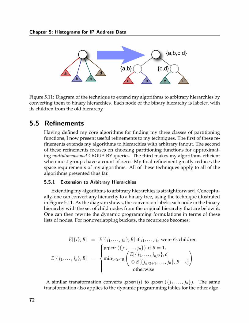
Chapter 5: Histograms for IP Address Data
dcb
aa,b c,d
a,b,c,d
ba dc
Figure 5.11: Diagram of the technique to extend my algorithms to arbitrary hierarchies byconverting them to binary hierarchies. Each node of the binary hierarchy is labeled withits children from the old hierarchy.
5.5 RefinementsHaving defined my core algorithms for finding my three classes of partitioningfunctions, I now present useful refinements to my techniques. The first of these re-finements extends my algorithms to hierarchies with arbitrary fanout. The secondof these refinements focuses on choosing partitioning functions for approximat-ing multidimensional GROUP BY queries. The third makes my algorithms efficientwhen most groups have a count of zero. My final refinement greatly reduces thespace requirements of my algorithms. All of these techniques apply to all of thealgorithms presented thus far.
5.5.1 Extension to Arbitrary Hierarchies
Extending my algorithms to arbitrary hierarchies is straightforward. Conceptu-ally, one can convert any hierarchy to a binary tree, using the technique illustratedin Figure 5.11. As the diagram shows, the conversion labels each node in the binaryhierarchy with the set of child nodes from the original hierarchy that are below it.One can then rewrite the dynamic programming formulations in terms of theselists of nodes. For nonoverlapping buckets, the recurrence becomes:
E[i, B] = E[ j1, . . . , jn, B] if j1, . . . , jn were i’s children
E[ j1, . . . , jn, B] =
grperr ( j1, . . . , jn) if B = 1,
min1≤c≤B
(E[ j1, . . . , jn/2, c]⊕ E[ jn/2+1, . . . , jn, B− c]
)otherwise
A similar transformation converts grperr(i) to grperr ( j1, . . . , jn). The sametransformation also applies to the dynamic programming tables for the other algo-
72

5.5 Refinements
rithms.
The number of interior nodes in the graph is still O(|G|) after the transfor-mation, so the transformation does not increase the order-of-magnitude runningtime of the nonoverlapping buckets algorithm. For the overlapping and longest-prefix-match algorithms, the longest path from the root to the leaves increases bya multiplicative factor of O(log(fanout)), increasing “big-O” running times by afactor of log2(fanout)).
73

Chapter 5: Histograms for IP Address Data
5.5.2 Extension to Multiple Dimensions
This chapter so far has dealt with queries over single-dimensional streams ofunique identifiers:
select G.GroupId, AGG(...)from UIDStream U [range ... slide ...],
GroupTable Gwhere G.uid = U.uidgroup by G.GroupId;
Some network monitoring applications require a variant of this query thatbreaks down traffic according to multiple unique identifiers:
select G1.gid, G2.gid, AGG(...)from UIDStream U [sliding window],
GroupTable G1,GroupTable G2
where G1.uid = U.uid1and G2.uid = U.uid2
group by G.GroupId;
The most common application of such multidimensional queries is breaking downtraffic by source and destination subnet. Other examples include tracking the rela-tionship between subnet and DNS name or between country and web URL. In thissection, I extend my algorithms to support building histograms that approximatethese multidimensional queries.
My histograms extend naturally to multiple dimensions while still finding op-timal histogram partitioning functions in polynomial time for a given dimension-ality. In d dimensions, I define a bucket as an d-tuple of hierarchy nodes. I assumethat there is a separate hierarchy for each of the d dimensions. Each bucket coversthe rectangular region of space defined by the ranges of its constituent hierarchynodes. Figure 5.12 illustrates a single bucket of a two-dimensional histogram builtusing this method. I denote the rectangular bucket region for nodes i1 through idas r(i1, . . . , id).
The extension of the non-overlapping buckets algorithm to d dimensions usesa dynamic programming table with entries in the form E[(i1, . . . , id), B], where i1through id are nodes of the d UID hierarchies. Each entry holds the best possibleerror for r(i1, . . . , id) using a total of B buckets. I also define a version of grperr that
74

5.5 Refinements
Root
0xx 1xx
11x
000 001 010 011 100 101 110 111
Root
0xx
1xx
11x
000
001
010
011
100
101
110
111
BucketNodes
0xxBucket
0xx
1xx
11x
Bucket
src_ip
dest
_ip
Figure 5.12: Diagram of a single bucket in a two-dimensional hierarchical histogram. Thebucket occupies the rectangular region at the intersection of the ranges of its bucket nodes.
aggregates over the region r(i1, · · · , id): grperr (i1, . . . , id)
E[(i1, . . . , id), B] is computed based on the entries for all subregions ofr(i1, . . . , id), in all combinations that add up to B buckets. For a two-dimensionalbinary hierarchy, the dynamic programming recurrence is shown below.Intuitively, the algorithm considers each way to split the region (i, j) in half alongone dimension. For each split dimension, the algorithm considers every possibleallocation of the B bucket nodes between the two halves of the region.
E[(i1, i2), B] =
grperr(i1, i2) if B = 1,
min
min1≤c≤BE[(i1, 2i2), c]⊕ E[(i1, 2i2 + 1), B− c]min1≤c≤BE[(2i1, i2), c]⊕ E[(2i1 + 1, i2), B− c]
otherwise
The extension of the overlapping buckets algorithm to multiple dimensionsis similar to the extension of the nonoverlapping algorithm. I make explicit theconstraint, implicit in the one-dimensional case, that every bucket region in a givensolution be strictly contained inside its parent region, with no partial overlap. For
75
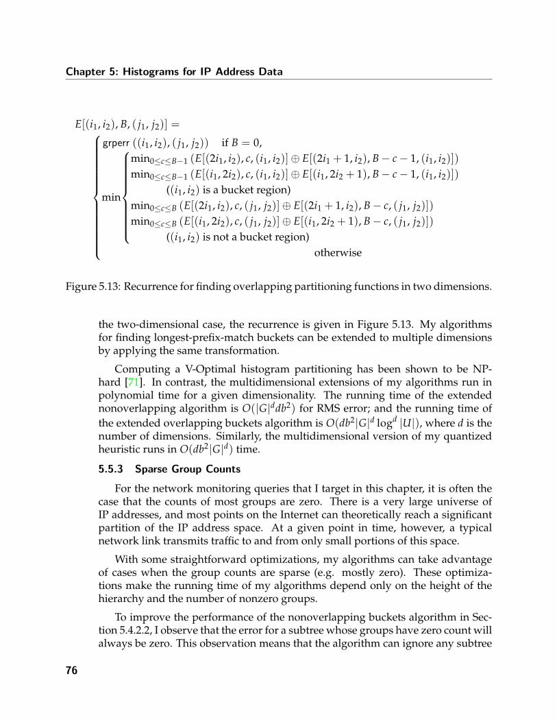
Chapter 5: Histograms for IP Address Data
E[(i1, i2), B, ( j1, j2)] =
grperr ((i1, i2), ( j1, j2)) if B = 0,
min
min0≤c≤B−1 (E[(2i1, i2), c, (i1, i2)]⊕ E[(2i1 + 1, i2), B− c− 1, (i1, i2)])min0≤c≤B−1 (E[(i1, 2i2), c, (i1, i2)]⊕ E[(i1, 2i2 + 1), B− c− 1, (i1, i2)])
((i1, i2) is a bucket region)min0≤c≤B (E[(2i1, i2), c, ( j1, j2)]⊕ E[(2i1 + 1, i2), B− c, ( j1, j2)])min0≤c≤B (E[(i1, 2i2), c, ( j1, j2)]⊕ E[(i1, 2i2 + 1), B− c, ( j1, j2)])
((i1, i2) is not a bucket region)otherwise
Figure 5.13: Recurrence for finding overlapping partitioning functions in two dimensions.
the two-dimensional case, the recurrence is given in Figure 5.13. My algorithmsfor finding longest-prefix-match buckets can be extended to multiple dimensionsby applying the same transformation.
Computing a V-Optimal histogram partitioning has been shown to be NP-hard [71]. In contrast, the multidimensional extensions of my algorithms run inpolynomial time for a given dimensionality. The running time of the extendednonoverlapping algorithm is O(|G|ddb2) for RMS error; and the running time ofthe extended overlapping buckets algorithm is O(db2|G|d logd |U|), where d is thenumber of dimensions. Similarly, the multidimensional version of my quantizedheuristic runs in O(db2|G|d) time.
5.5.3 Sparse Group Counts
For the network monitoring queries that I target in this chapter, it is often thecase that the counts of most groups are zero. There is a very large universe ofIP addresses, and most points on the Internet can theoretically reach a significantpartition of the IP address space. At a given point in time, however, a typicalnetwork link transmits traffic to and from only small portions of this space.
With some straightforward optimizations, my algorithms can take advantageof cases when the group counts are sparse (e.g. mostly zero). These optimiza-tions make the running time of my algorithms depend only on the height of thehierarchy and the number of nonzero groups.
To improve the performance of the nonoverlapping buckets algorithm in Sec-tion 5.4.2.2, I observe that the error for a subtree whose groups have zero count willalways be zero. This observation means that the algorithm can ignore any subtree
76

5.5 Refinements
EmptySubtree
Single-GroupBucket
zerocount
zerocount
nonzerocount
Figure 5.14: One of the sparse buckets that allow my overlapping histograms to representsparse group counts efficiently. Such a bucket produces zero error and can be representedin O(log log |U|) more bits than a conventional bucket.
whose leaf nodes all have a count of zero. Furthermore, the system does not needto store any information about buckets with counts of zero, as these buckets can beeasily inferred from the non-empty buckets on the fly.
For overlapping and longest-prefix-match buckets, I introduce a new class ofbucket, the sparse bucket. A sparse bucket consists of a single-group sub-bucket andan empty subtree that contains it, as shown in Figure 5.14. As a result, the ap-proximation error within a sparse bucket is always zero. Since the empty subtreehas zero count and can be encoded as a distance up the tree from the sub-bucket,a sparse bucket takes up only O(log log |U|) more space than a single normalbucket.
A sparse bucket dominates any other solution that places bucket nodes in itssubtree. As a result, my overlapping buckets algorithm does not need to considerany such solutions when it can create a sparse bucket. Dynamic programming canstart at the upper node of each candidate sparse bucket. Since there is one candi-date sparse bucket for each nonzero group, the algorithm runs in O(gb2 log |U|)time, where g is the number of nonzero groups.
For my target monitoring applications, it is important to note that the timerequired to produce an approximate query answer from one of my histograms isproportional to the number of groups the histogram predicts will have nonzerocount. Because of this relationship, the end-to-end running time of the system canbe sensitive to how aggressively the histogram marks empty ranges of the UIDspace as empty. Error metrics that penalize giving a zero-count group a nonzerocount will make the approximate group-by query run much more quickly.
77

Chapter 5: Histograms for IP Address Data
5.5.4 Space Requirements
A naive implementation of my algorithms would require large in-memory ta-bles. However, a simple technique developed by Guha [43] reduces the memoryoverhead of the algorithms to very manageable sizes. The basic strategy is to com-pute only the error and number of buckets on the left and right children at the rootof the tree. Once entry E[i, · · · ] has been used to compute all the entries for nodeb i
2c, the entry can be garbage-collected.
To reconstruct the entire bucket set, the technique uses a divide-and-conquerstrategy: First, run the algorithm over the entire hierarchy to determine how manybucket nodes are in the root’s left and right subtrees, then recurse on those sub-trees. This technique divides the original problem into two subproblems, each ofwhich is half the size of the original problem. To further reduce memory require-ments, the nodes themselves could be stored on disk in this order and read intomemory as needed. In the worst case, it takes O(log |U|) passes (one pass for eachlevel of the hierarchy) of divide-and-conquer to reconstruct the entire solution.
When Guha’s technique is applied to my algorithm for finding nonoverlap-ping partitioning functions for RMS error, each round of subproblems takes a totalof O(|G|(b2 + log |U|)) time. So the overall running time of the nonoverlappingalgorithm increases to O(|G| log |U|(b2 + log |U|)). Likewise, the running time ofmy algorithm for finding overlapping partitioning functions also increases by afactor of log |U| to O(|G|b2 log2 |U|) time. As Guha notes, algorithms that requireO(|G|2) or more time will see no increase in running time when his technique isapplied. My algorithms for finding longest-prefix-match partitioning functions, aswell as my multidimensional algorithms, all fall into this category.
In my actual implementation, I use a less aggressive form of pruning that avoidthe O(log |U|) increase in running time of Guha’s technique. My implementationprunes all elements of the table except those that are part of the optimal solutionto a subproblem at the current level of the hierarchy under consideration. Whendynamic programming reaches the root of the hierarchy, the optimal set of bucketnodes can be reconstructed as if the entire table were in memory. Theoretically,this technique may not prune any table entries at all. In my experiments, however,the technique results in a space reduction comparable to that of Guha’s technique,without requiring multiple passes to recover the bucket nodes. Intuitively, thepartial solutions for a given subtree tend to overlap; the best b-bucket solutionfor a subtree will share most of its bucket nodes (and hence most of its optimalsub-problems) with the best b− 1-bucket solution, and so on.
The number of table entries that must be kept in memory at a given time isalso a function of the order in which the algorithm processes the nodes of the UIDhierarchy. The maximum working set size of my algorithms can be minimized by
78

5.5 Refinements
Next node
of traversal
Nodes whose table
entries can be
garbage-collectedNodes whose table entries
are in main memory
Figure 5.15: Illustration of garbage-collecting unneeded table entries during a preordertraversal of the hierarchy. At most, the algorithms in this chapter need to keep entries forone node from each level of the hierarchy at a given time.
processing nodes in the order of a preorder traversal, keeping the memory foot-print to a minimum. At a given point in the preorder traversal, a pass of dynamicprogramming will be considering table entries associated with the nodes alonga cut in the hierarchy that contains at most one node from each level, as illus-trated in Figure 5.15. There are O(log |U|) such nodes at any time (assuming abalanced UID hierarchy), and the only table entries that need to be in memory arethe ones for the nodes along the cut. Since my nonoverlapping algorithm has btable entries for each node, the algorithm needs to keep only O(b log |U|) table en-tries in memory at a time. Similarly, my overlapping partitions algorithm requiresO(b log2 |U|) space. My quantized heuristic requires O(k3b log2 |U|) space, wherek is the number of quanta for each counter.
79

Chapter 5: Histograms for IP Address Data
0.1
1
10
100
1000
10000
100000
1e+06
4 8 12 16 20 24 28 32
Num
ber o
f Sub
nets
(Log
Sca
le)
Prefix Length
Maximum
Possible
Figure 5.16: The distribution of IP prefix lengths in my experimental set of subnets. Thedotted line indicates the number of possible IP prefixes of a given length (2length). Jumpsat 8, 16, and 24 bits are artifacts of an older system of subnets that used only three prefixlengths.
5.6 Experimental EvaluationTo measure the effectiveness of my techniques, I conducted a series of evaluationson real network monitoring data and metadata.
The WHOIS databases store ownership information on publicly accessiblesubnets of the Internet. Each database serves a different set of addresses,though WHOIS providers often mirror each others’ entries. I downloadedpublicly-available dumps of the RIPE and APNIC WHOIS databases [90, 5] andmerged them, removing duplicate entries. I then used this table of subnets togenerate a table of 1.1 million nonoverlapping IP address prefixes that completelycover the IP address space. Each prefix corresponds to a different subnet. Theprefixes ranged in length from 3 bits (536 million addresses) to 32 bits (1 address),with the larger address ranges denoting unused portions of the IP address space.Figure 5.16 shows the distribution of prefix lengths.
I obtained a large trace of “dark address” traffic on a slice of the global Internet.The destinations of packets in this trace are IP addresses that are not assigned toany active subnet. The trace contains 7 million packets from 187866 unique sourceaddresses. Figure 5.17 gives a breakdown of this traffic according to the subnets inmy subnet table.
I chose a query that counts the number of packets in each subnet:
select S. id , count(∗)
80

5.6 Experimental Evaluation
Figure 5.17: The distribution of network traffic in my trace by source subnet. Due toquantization effects, most ranges appear wider than they actually are. Note the logarith-mic scale on the Y axis.
fromPacket P,Subnet S
where−− Adjacent table entries with the same subnet−− are merged into a single table entryP. src ip ≥ I . id and P.src ip ≤ I . id
group by S.id
I used six kinds of histogram to approximate the results of this query:
• Hierarchical histograms with nonoverlapping buckets
• Hierarchical histograms with overlapping buckets
• Hierarchical histograms with longest-prefix-match buckets, generated with thegreedy heuristic
• Hierarchical histograms with longest-prefix-match buckets, generated with thequantized heuristic
• End-biased histograms [50]
• V-Optimal histograms [52]
81

Chapter 5: Histograms for IP Address Data
An end-biased histogram consists of a set of single-group buckets for the b− 1groups with the highest counts and a single multi-group bucket containing thecount for all remaining groups. I chose to compare against this type of histogramfor several reasons. End-biased histograms are widely used in practice. Also, con-struction of these histograms is tractable for millions of groups, and my data setcontained 1.1 million groups. Additionally, end-biased histograms model skeweddistributions well, and the traffic in my data set was concentrated in a relativelysmall number of groups.
A V-Optimal histogram is an optimal histogram where each bucketcorresponds to an arbitrary contiguous range of values. For RMS error, theV-Optimal algorithm of Jagadish et al.[52] can be adapted to run in O(|G|2) time,where G is the set of nonzero groups. For an arbitrary distributive error metric,the algorithm takes O(|G|3) time, making it unsuitable for the sizes of data set Iconsidered. I therefore used RMS error to construct all the V-Optimal histogramsin my study.
I studied the four different error metrics discussed in Section 5.3.2.3:
• Root Mean Square (RMS) error
• Average error
• Average relative error
• Maximum relative error
Note that these errors are computed across vectors of groups in the result of thegrouped aggregation query, not across vectors of histogram buckets.
For each error metric, I constructed hierarchical histograms that minimize theerror metric. I compared the error of the six histogram types, repeating the experi-ment at histogram sizes ranging from 10 to 20 buckets in increments of 1 and from20 to 1000 buckets in increments of 10.
5.6.1 Experimental Results
I divide my experiment results according to the type of error metric used. Foreach error metric, I give a graph of query result estimation error as a function ofthe number of histogram buckets. The dynamic range of this error can be as muchas two orders of magnitude, so the y axes of my graphs have logarithmic scales.
5.6.1.1 RMS Error
My first experiment measured RMS error. The RMS error formula empha-sizes larger deviations, making it sensitive to the accuracy of the groups withthe highest counts. Longest-prefix-match histograms produced with the greedy
82

5.6 Experimental Evaluation
100
1000
0 50 100 150 200 250 300 350 400 450 500
RM
S E
rro
r(L
og
Sca
le)
Number of Buckets
Nonoverlapping
Overlapping
Greedy
Quantized
End-BiasedV-Optimal
Figure 5.18: RMS error in estimating the results of my query with the different histogramtypes.
heuristic were the clear winner, by virtue of their ability to isolate these “outlier”groups inside nested partitions. Interestingly, the quantized heuristic fared rela-tively poorly in this experiment, finishing at the middle of the pack. The heuris-tic’s logarithmically-distributed counters were unable to capture sufficiently fine-grained information to produce more accurate results than the greedy heuristic.
5.6.1.2 Average Error
My second experiment used average error as an error metric. Figure 5.19 showsthe results of this experiment. As with RMS error, the greedy heuristic producedthe lowest error, but the V-Optimal histograms and the quantized heuristic pro-duced results that were almost as good. Average error puts less emphasis ongroups with very high counts, and these heuristics emphasize such outliers in theirpartition choices. The other types of histogram produced significantly higher er-ror. As before, I believe this performance difference is mainly due to the ability oflongest-prefix-match and V-Optimal histograms to isolate outliers by putting theminto separate buckets.
5.6.1.3 Average Relative Error
My third experiment compared the three histogram types using average rela-tive error as an error metric. Compared with the previous two metrics, relativeerror emphasizes errors on the groups with smaller counts. Figure 5.20 shows theresults of this experiment. The quantized heuristic produced the best histograms
83

Chapter 5: Histograms for IP Address Data
10
100
1000
0 50 100 150 200 250 300 350 400 450 500
Ave
rag
e E
rro
r(L
og
Sca
le)
Number of Buckets
Nonoverlapping
Overlapping
Greedy
Quantized
End-Biased
V-Optimal
Figure 5.19: Average error in estimating the results of my query with the different his-togram types.
for this error metric. The heuristic’s quantized counters were better at trackinglow-count groups than they were at tracking the larger groups that dominated theother experiments. V-Optimal histograms produced low error at smaller bucketcounts, but fell behind as the number of buckets increased.
5.6.1.4 Maximum Relative Error
My final experiment used maximum relative error. This error metric measuresthe ability of a histogram to produce low error for every group at once. Resultsare shown in Figure 5.21. Histograms with overlapping partitioning functionsproduced the lowest result error for this error measure. Interestingly, the greedyheuristic was unable to find good longest-prefix-match partitioning functions forthe maximum relative error measure. Intuitively, the heuristic assumes that re-moving a hole from a partition has no effect on the mean count of the partition.Most of the time, this assumption is true; however, when it is false, the resultinghistogram can have a large error in estimating the counts of certain groups. Sincethe maximum relative error metric finds the maximum error over the entire set ofgroups, a bad choice anywhere in the UID hierarchy will corrupt the entire parti-tioning function.
84

5.6 Experimental Evaluation
1
10
100
0 50 100 150 200 250 300 350 400 450 500
Ave
rag
e R
ela
tive
Err
or
(Lo
g S
ca
le)
Number of Buckets
Nonoverlapping
Overlapping
Greedy
Quantized
End-Biased
V-Optimal
Figure 5.20: Average relative error in estimating the results of my query with the differenthistogram types. Longest-prefix-match histograms significantly outperformed the othertwo histogram types.
10
100
1000
10000
100000
0 50 100 150 200 250 300 350 400 450 500
Ma
xim
um
Re
lative
Err
or
(Lo
g S
ca
le)
Number of Buckets
Nonoverlapping
Overlapping
Greedy
QuantizedEnd-Biased
V-Optimal
Figure 5.21: Maximum relative error in estimating the results of my query with the differ-ent histogram types.
85

86

Chapter 6
Deployment Study
Good judgment comes from experience, and experience comes from bad judgment.
— Barry LePatner
87

Chapter 6: Deployment Study
6.1 IntroductionThis chapter presents a detailed performance study of the Data Triage architec-
ture in the context of an end-to-end network monitoring system. The system inquestion arose from a collaboration between myself and researchers at LawrenceBerkeley National Laboratory. The high-level aim of this collaboration was to builda software platform for monitoring the network traffic of the Department of Engi-neering national laboratories.
From the perspective of this dissertation, the study had several goals:
• Demonstrate the feasibility of using a general-purpose streaming query proces-sor to monitor high-speed networks
• Show that Data Triage is necessary to maintain low query result latency in sucha context
• Demonstrate that my prototype implementation of Data Triage can scale to sup-port a “real-world” workload
• Show that the extension of Data Triage for archived streams as described inSection 3.4 also works in such a setting
6.2 BackgroundThe United States Department of Energy (DOE) operates nine major research labsnationwide. These laboratories conduct classified and unclassified research in ar-eas such as high-energy physics, nuclear fusion and climate change. Researchersat the labs regularly collaborate with major university and industrial research or-ganizations. To support collaborations both between the labs and with outsideresearchers, each lab maintains high-speed network connections to several nation-wide networks. In addition, each lab publishes large amounts of information viaits connection to the public Internet.
The security of these network connections is crucial to operations at the DOElabs. As a U.S. government agency, the Department of Energy is a prime target ofmalicious hackers worldwide. The laboratories need to protect sensitive informa-tion and to prevent illegal misuse of their equipment.
Network availability and performance are another important priority at DOE.Large data transfers are an integral part of many important projects at the labs.Multimillion-dollar particle accelerators cannot run unless enough network band-width is available to absorb their data streams. DOE scientists running simulationsroutinely ship large data sets across the world, and increased use of grid comput-
88

6.2 Background
Query
Processor
Historical
Data
Network
AdminOperations
Center
Backbone
Network
Flow Monitors
Network Links(Nationwide)
Flow
Records
Figure 6.1: High-level block diagram of the proposed nationwide network monitoringinfrastructure for the DOE labs.
ing is making network uptime even more essential.
To help maintain network security, availability, and performance at its labora-tories, DOE is creating a nationwide network operations center. This centralizedmonitoring station will enable a small team of network administrators to maintaina 24-hour alert for potential problems. Figure 6.1 illustrates how this system willwork. At each laboratory, TCP/IP flow monitors collect information about networksessions and stream the resulting flow records to the operations center via a back-bone link. Software at the operations center aggregates and analyzes the streamsof flow records to present a real-time picture to the human operators on the scene.
This chapter describes my experiences working with researchers at LawrenceBerkeley National Laboratories to build a prototype of the analysis software thatcould be run at the network operations center. We identified three key require-ments for this software:
• Flexibility: The network operator needs to focus analysis on the machines, pat-
89

Chapter 6: Deployment Study
terns, and protocols that are relevant to the problem at hand. He or she willalso need to develop and deploy new analyses quickly in response to evolvingthreats.
• History: An effective monitoring system needs access to historical data aboutthe network. This past history allows the operator to weed out false positivesby comparing present behavior against past behavior. History is also essentialfor determining the cause of a malfunction or security breach that occurred inthe past.
• Performance: During periods of peak load, the DOE networks each generatetens of thousands of flow records per second. It is during these peak periodsthat effective network monitoring is most essential. High traffic puts stresses onthe network that make it more likely to fail. Also, knowledgeable adversarieswill attempt to hide their attacks inside these large bursts of data.
My collaborators have been working on FastBit [11, 101], a high-performancebitmap index with a declarative SQL interface. Working with the FastBit team, I de-signed an end-to-end system that uses TelegraphCQ for streaming query process-ing and FastBit to provide access to historical data. This design easily meets ourfirst two requirements, since TelegraphCQ and FastBit both use flexible declarativequery languages and FastBit provides access to historical data. Our main questiongoing forward was whether the combination of these two general-purpose systemscan handle sufficiently high data rates to meet the performance requirement.
6.2.1 Data Rates
The total traffic on the Department of Energy’s networks is classified, but wecan make a rough estimate based on unclassified data. We have obtained flowrecords from Berkeley Lab’s unclassified NERSC (National Energy Research Sci-entific Computing) Center for a 42-week period from August 2004 through June2005.
Figure 6.2 shows the number of flows (or network sessions) per week duringthis period. During the trace, the network generated as many as 250 million flowrecords in a week, or 500 records/sec on average. However, the rate at whichthese flows arrived varied significantly, reaching as high as 55,000 flow recordsper second as shown in Figure 6.3. This figure shows the histogram of flow recordrates. We observed that this distribution is heavy-tailed.
The NERSC traffic is one of three wide-area network links currently deployedat Berkeley Lab, and the lab’s employees represent about one tenth of all DOElab researchers. Assuming that other network links have approximately the sametraffic levels as the NERSC link and that network usage scales with the number ofresearchers, we therefore expect the NERSC link to represent approximately 1/30
90

6.2 Background
Figure 6.2: Flow records per week in our 42-week snapshot of Berkeley Lab’s connectionto the NERSC backbone.
of the total DOE traffic. So a DOE-wide network operations center would needto process sustained rates of roughly 500 × 30 = 15, 000 flow records per second,with peaks of as much as 55, 000× 30 = 1, 650, 000 records per second.
6.2.2 Query Complexity
Based on a literature survey and my own conversations with networking re-searchers, I developed a sample workload of queries for monitoring networks. Idescribe this workload in detail in Section 6.5. Each of my queries has a live stream-ing component and a historical archive component. The live component of eachquery monitors the current status of the network. The historical parts analyze pre-vious flow records to trace problems back to their roots or to determine whetherpotential anomalies are actually normal behavior. Running these queries requiresreal-time analysis and fast index access to as much as a month of historical data.A real deployment would run a mix of 10 to 100 such queries, monitoring various
91

Chapter 6: Deployment Study
1e-12 1e-11 1e-10 1e-09 1e-08 1e-07 1e-06 1e-05 1e-04 0.001 0.01 0.1
0 10000 20000 30000 40000 50000 60000
Prob
abilit
y De
nsity
(log
scal
e)
Flow Records/SecFigure 6.3: Histogram of the number of flow records per second in the data set in Fig-ure 6.2. The distribution is heavy-tailed, with a peak observed rate of 55,000 records persecond.
aspects of the network in real time.
6.2.3 Analyzing The Performance Problem
Based on my earlier experience with smaller prototypes, I hypothesized thatTelegraphCQ would be the major bottleneck in our combined system and that thesystem would need Data Triage to provide reasonable response times in the faceof bursty network traffic. I worked with the FastBit team to design a performancestudy that would break down the performance of the system in terms of both datathroughput and query result latency. The Berkeley Lab researchers optimized theFastBit engine and tweaked the historical components of my query workload forbetter performance. I debugged and performance tuned TelegraphCQ, as well asadding query language support for my query workload. I also created a robusthigh-performance implementation of Data Triage to match the performance-tunedTelegraphCQ. Then I wrote and optimized the code that ties these three compo-nents together. I designed a set of experiments that break down system perfor-mance in terms of the individual components of the system, as well as end-to-endexperiments for evaluating the entire system. The FastBit team measured the per-formance of the FastBit component of our system. I measured the performanceof TelegraphCQ by itself, both with and without my Data Triage implementation.Finally, I ran experiments that measured the performance of the entire system. The
92

6.3 Architecture
Staging
Area
Query Results
Network
Admin
Summarizer
Triage Queue
Flow
Records
FastBit
Index
TelegraphCQ
Engine
FastBit
Loader
FastBit
Runtime
Application
Logic
DBI
Library
Ingress Manager
Reorder
Controller
Figure 6.4: Block diagram of our network monitoring prototype. Our system combinesthe data retrieval capabilities of FastBit with the stream query processing of TelegraphCQ.
remainder of this chapter describes the steps of our performance study in detail,starting with my overall design and data/query workload and then describing ourexperimental results.
6.3 ArchitectureThis section gives a high-level overview of the architecture I designed for our pro-totype monitoring system and provides references for further reading on individ-ual components of our system. Figure 6.4 shows how the pieces of our architecturefit together. The major components of the system are as follows:
TelegraphCQ is a streaming query processor that filters, categorizes, and ag-gregates flow records according to one or more continuous queries, generatingperiodic reports. I give an overview of TelegraphCQ in Section 1.6 of this disserta-tion.
FastBit is a bitmap index system with an SQL interface. It is designed to workwith append-only data sets such as historical records of a network monitoring sys-tem. My design uses FastBit to provide fast associative access to archived networkmonitoring data. The keys to FastBit’s efficiency are its vertical data organizationand efficient bitmap compression algorithms [96, 114, 115].
The Ingress Manager component corresponds to the Triage Process in my de-sign for Data Triage with archival data (See Section 3.4). The Ingress Manager pro-cess contains a Triage Queue, Triage Scheduler, and Summarizer, as well as codethat stages data to disk for loading into FastBit. This component also merges in-coming streams of flow records and converts data into formats that TelegraphCQ
93

Chapter 6: Deployment Study
Week Records/week Cumulative no. of records
1 49,289,726 49,289,7262 17,826,252 67,115,9783 22,315,221 89,431,1994 11,402,761 100,833,9605 20,256,664 121,090,624
Table 6.1: Number of network traffic records collected at Berkeley Lab over a period of 5weeks.
and FastBit understand.
The Controller is a component that receives streaming query results from Tele-graphCQ, requests relevant historical data from the FastBit index, and generatesconcise reports for the network administrator. Each analysis that the controllerperforms consists of three parts: A TelegraphCQ query template, a FastBit querytemplate, and application logic. The Controller reads TelegraphCQ and FastBitquery templates from configuration files and substitutes in runtime parameters.The application logic for an analysis consists of a callback that is invoked for eachbatch of query results that comes back from TelegraphCQ. Each analysis runs ina separate process, but the Controller’s admission control limits the number ofconcurrent FastBit queries to prevent thrashing.
The Controller is currently implemented in the Perl programming language. Ichose Perl because it has an efficient interface with TelegraphCQ, dynamic com-pilation for loading application logic at runtime, and well-developed facilities forgenerating reports.
6.4 DataAll our performance benchmarks are based on real network connection datathat researchers at Berkeley Lab collected on the Lab’s NERSC supercomputingbackbone connection. The data represents a time period of 5 weeks and consistsof 121 million TCP/IP flow records. Each flow record contains information on thesource/destination IP addresses, source/destination ports, time stamp, packetsize, etc. In total, each record contains 11 attributes.
Table 6.1 shows the number of network traffic records per week along with thecumulative number of records. Note that week 1 comprises about 5 times morerecords than week 4.
I mapped the attributes in the flow records into the following TelegraphCQstream:
94

6.4 Data
create stream Flow(src ip Inet,dst ip Inet,src port integer,dst port integer,protocol integer, −− Protocol numberbytes sent integer, −− src−>dstbytes recv integer, −− dst−>srcoutgoing boolean,
−− TRUE if this connection was initiated−− inside the protected network
state integer,−− Where in the TCP state machine the−− connection ended up.
duration interval ,tcqtime timestamp TIMESTAMPCOLUMN
)type unarchived;
Recall from Section 1.6 that TelegraphCQ create stream statements are similarto SQL create table statements. The text type unarchived at the end of the state-ment indicates that the TelegraphCQ is not to archive flow records internally; mysystem design uses FastBit for all archival storage. The Inet data type is a built-in PostgreSQL type for storing IP addresses; other types used in this schema arenative SQL92 types.
To store the historical flow records, my LBNL collaborators created acorresponding FastBit table. FastBit’s queries operate over a single vertically-partitioned table, with columns stored in separate files. Individual columnsvalues are stored in native C++ data types. Table 6.2 summarizes the mappingbetween our FastBit and TelegraphCQ schemas.
95

Chapter 6: Deployment Study
TCQ Column FastBit Column(s) C++ Type
src ip IPS intdst ip IPR intsrc port SP intdst port DP intprotocol PROT intbytes sent S SIZE intbytes recv R SIZE intoutgoing FLAG intstate STATE intduration dur doubletcqtime ts int
Table 6.2: Relationship between columns of our TelegraphCQ and FastBit schemas
6.5 QueriesBased on a literature search and discussions with networking researchers, I havecreated a representative workload of real-time network analyses. Each analysis iscomprised of a stream query processing component, expressed as a TelegraphCQquery; and a historical component, expressed as a FastBit query. These queriesrepresent an important contribution: To my knowledge, no other collection of sim-ilarly complex live/archive queries for network monitoring has been publishedin the data management, streaming query processing, or network measurementliterature.
In the sections that follow, I present these queries in the native query languagesof TelegraphCQ and FastBit, respectively, using the schemas from Section 6.4.
Each query has one or more parameters that are bound at runtime. Followingthe convention of most SQL databases, I denote these variable parameters with apreceding colon. For example, in the first “elephants” query below, the parameter:windowsz is variable. At runtime, the Controller component of the system substi-tutes the appropriate values for for the variable parameters in the templates.
6.5.1 Elephants
Goal: This analysis finds the k most significant sources of traffic (source/desti-nation pairs, subnets, ports, etc.)1. TelegraphCQ finds the top k, and FastBit com-pares these top k against their previous history. Reports significant traffic sources
1The names of this query and the one that follow derive from the networking term “elephants and mice”, which refers to thesources of the largest and smallest traffic on a network link, respectively. “Elephants” tend to dominate bandwidth usage, andsecurity problems often involve “mice”.
96

6.5 Queries
that were not significant in the past.
TelegraphCQ Query: Finds top 100 addresses by data sent.
select sum(bytes sent), src ip , wtime(∗) as nowfrom flow [range by :windowsz slide by :windowsz]where outgoing = falsegroup by src iporder by sum(bytes sent) desclimit 100 per window;
FastBit Query: Retrieves the total traffic from the indicated 100 addresses forthe same time of day over the past 7 days. The variables :X1, :X2 and so on are thesrc ip output from the above TelegraphCQ query. Note also that FastBit querieshave an implicit GROUP BY clause on all selected attributes that are not part of anyaggregate functions.
select IPS, sum(S SIZE), sum(R SIZE)where IPS in (:X1, :X2, :X3, ..., :X100) and(( ts between [:now − 24 hr] and [:now − 23 hr])or (ts between [:now − 48 hr] and [:now − 47 hr])or (ts between [:now − 72 hr] and [:now − 71 hr])or (ts between [:now − 96 hr] and [:now − 95 hr])or (ts between [:now − 120 hr] and [:now − 125 hr])or (ts between [:now − 144 hr] and [:now − 143 hr])or (ts between [:now − 168 hr] and [:now − 167 hr]));
6.5.2 Mice
Goal: Find all traffic from hosts that have not historically sent large amountsof traffic. FastBit finds the top k hosts by bytes sent over the past week. ThenTelegraphCQ looks for traffic that is not from these top k hosts.
FastBit Query: Retrieves the top k hosts by total traffic for the past week. Thevariable : history , called the length of history, defines how far back in history thequery looks for historical patterns. We usually vary its value from a few days to amonth.
select sum(S SIZE), IPSwhere ts between [:now − :history] and [:now]order by sum(S SIZE) desc
97

Chapter 6: Deployment Study
limit :k;
TelegraphCQ Query: Produces a breakdown of traffic that is not from the hostsin the FastBit query’s results.
select sum(bytes sent), src ip , dst ip , wtime(∗)from flow [range by :windowsz slide by :windowsz]where
src ip != :X1 and src ip != :X2 and ... and src ip != :X100group by src ip , dst iporder by sum(bytes sent) desclimit 100 per window;
6.5.3 Portscans
Goal: This analysis finds behavior that suggests port scanning activity2. Tele-graphCQ flags current behavior, and FastBit is used to filter out hosts that exhibitthis behavior as part of normal traffic.
TelegraphCQ Query: Finds external hosts that connect to many distinct desti-nations and ports within Berkeley Lab. The ORDER BY and LIMIT clause at the endof the query indicates that TelegraphCQ should return the top 100 hosts accordingto “fanout”.
select src ip ,count(distinct ( dst ip :: varchar || dst port :: varchar)) as fanout,wtime(∗)
from flow [range by :windowsz slide by :windowsz]where outgoing = falsegroup by src iporder by fanout desclimit 100 per window;
FastBit Query: Given the IP addresses returned by the TelegraphCQ query( :X1 through :X100), this query determine which hosts those addresses have his-torically communicated with. Application logic can use this information to differ-entiate between suspicious behavior and normal traffic patterns.
Note that FastBit queries with no aggregates have an implicit count(∗) aggre-
2A port is a numeric identifier within a single host that is associated with a single process running on the host. The termportscan refers to the common practice of making blind connection attempts to a remote host to determine which network portsare associated with running programs [112].
98

6.5 Queries
gate.
select IPR, IPSwhere
IPS in (:X1, :X2, :X3, ... , :X100)and (ts between [:now − :history] and [:now])
6.5.4 Anomaly detection
Goal: This analysis compares the current local traffic matrix (traffic bysource/destination pair) against a traffic matrix from the past. TelegraphCQfetches the current traffic matrix, and FastBit fetches the matrix in the past. Thenapplication logic compares the matrices using a change metric such as the L1norm or Euclidean distance. More sophisticated analyses involving multiplehistorical traffic matrices are also possible [99].
TelegraphCQ Query: Computes the local traffic matrix, merging the traffic inboth directions.
select(case when outgoing = truethen src ip else dst ip end) as inside ip ,(case when outgoing = truethen dst ip else src ip end) as outside ip ,sum(bytes sent) + sum(bytes recv) as bytes
from flow [range by :windowsz slide by :windowsz]group by inside ip , outside ip ;
FastBit Query: Fetches the incoming portion of the traffic matrix for a singleperiod of time.
selectIPS, sum(S SIZE)
whereoutgoing = falseand (ts between [:now − :history] and [:now])
order by sum(S SIZE) desc
6.5.5 Dispersion
Goal: This analysis finds subnets at a parametrizable IP prefix length that ap-pear in two time windows within a given period, and reports the time lag be-
99

Chapter 6: Deployment Study
tween these two windows. Certain patterns of time lag can indicate maliciousbehavior[22]. A TelegraphCQ query with two subqueries does the real-time analy-sis, and a FastBit query summarizes the traffic history for each IP prefix identified.This is based on a query in [22].
TelegraphCQ Query: Produces a breakdown of traffic by subnet. The parame-ter : prefixlen determines the length of the IP address prefix that defines a subnet.WTIME(∗) is a TelegraphCQ built-in function that returns the latest timestamp inthe current time window.
withWindowResults1 as(select
network(set masklen( src ip , : prefixlen )) as prefix ,wtime(∗) as tcqtime
from Flow [range by :windowsz slide by :windowsz]group by prefix)WindowResults2 as(
−− Create a second copy of the streamselect ∗ from WindowResults1
)(select
W1.prefix as prefix ,W2.tcqtime − W1.tcqtime as lag,count(∗),wtime(∗)
fromWindowResults1 W1 [range by 10 ∗ :windowsz
slide by :windowsz],WindowResults2 W2 [range by 10 ∗ :windowsz
slide by :windowsz]where W1.prefix = W2.prefix
and W2.tcqtime > W1.tcqtimegroup by W1.prefix, lag );
FastBit Query: Fetches the incoming traffic for the given subnets in the giventime window.
Ideally, this query would group results by network subnet as in theTelegraphCQ query above (e.g. select network(set masklen(IPS, : prefixlen ))).However, FastBit currently does not support arithmetic expressions in its select
100

6.6 Experiments
lists, so the query breaks down traffic by source address.
selectIPS, IPR, sum(R SIZE)
where( prefix (IPS, : prefixlen ) = :X1 OR ... = :X2 OR ... )and (ts between [:now − :history] and [:now])and outgoing = false
order by sum(R SIZE) desc
6.6 ExperimentsIn this section, I evaluate the performance of our system in a series of experiments.I start by analyzing the major components of the system separately to determinethe peak data throughput of each component. I then benchmark the throughput ofthe entire system and compare this end-to-end throughput against that of the indi-vidual components. Finally, I evaluate the performance of the system with realisticpacket arrival rates derived from the timestamps in Lawrence Berkeley NationalLab’s traces. All experiments were conducted on a server with dual 2.8 GHz Pen-tium 4 processors, 2 GB of main memory, and an IDE RAID storage system capableof sustaining 60 MB/sec for reads and writes.
6.6.1 TelegraphCQ Without Data Triage
My first experiment examined the performance tradeoffs of the TelegraphCQcomponent of the system without Data Triage. I focused on two parameters: querytype and window size. Recall that each of the five TelegraphCQ queries in myworkload produces results for discrete windows of time, and the size of these win-dows is given as a parameter in the query.
Bypassing the Data Triage components of the Ingress Manager, I sent week 5 ofthe trace directly through TelegraphCQ and measured the total running time foreach of my five TelegraphCQ queries. From this running time, the window size,and the number of tuples in the trace, I computed an average throughput figurefor the query processor. I repeated the experiment while varying the window sizefrom 1 to 1,000 seconds. This range of time intervals corresponds to an average ofbetween 38.1 and 38,114 tuples per time window.
Figure 6.5 shows the measured throughput of TelegraphCQ in my experiments.Each query showed an initial increase in throughput as window size increased. Aswindow size continued to increase, throughput eventually reached a peak anddeclined somewhat. The “dispersion” query showed a particularly pronouncedinstance of this pattern, with throughput increasing from 6,000 to 25,000 tuples
101

Chapter 6: Deployment Study
30000
20000
10000
5000 10 100 1000 10000 100000
Flo
w R
ecord
s/s
ec
(log s
cale
)
Average Number of Records per Window(log scale)
anomalydispersionelephants
miceportscans
Figure 6.5: The throughput of TelegraphCQ running my queries with varying windowsizes over the 5th week of the NERSC trace. Note the logarithmic scale.
across the range of window sizes targeted. The remaining queries had much flatterthroughput curves.
I profiled my TelegraphCQ testbed to determine the reason for the changesin throughput I observed. I found that the relatively low throughputs at smallerwindow sizes were due to the large number of result tuples the queries produce atthose window sizes. This effect was particularly pronounced with the dispersionquery because the results of the first subquery went into a self-join, which is a morecomplex operation than the rest. I traced the slight falloff in performance at largerwindow sizes to increased memory footprint, as TelegraphCQ buffers the tuplesin the current window in memory.
With the appropriate choice of window size, a single instance of TelegraphCQcan handle the average aggregate flow record traffic of all the DOE labs. A smallcluster of machines should be able to run a 10-20 query workload at this averagedata rate. It is important to note, however, that such a setup would buffer excessdata and return delayed query results whenever data rates exceeded the average.The experiments in Section 6.6.7 quantify this delay and explore methods for re-
102

6.6 Experiments
10000
100000
10 100 1000 10000 100000
Tupl
es/s
ec(lo
g sc
ale)
Average Number of Tuples per Window(log scale)
anomalydispersionelephants
miceportscans
Figure 6.6: The throughput of TelegraphCQ with Data Triage, running my queries withvarying window sizes over the 5th week of the NERSC trace. Note the logarithmic scale.
ducing it.
6.6.2 TelegraphCQ With Data Triage
My next experiment measured the peak throughput of the streaming compo-nent of the system when Data Triage is used. I used the same setup as the experi-ment in the previous section, except that the Data Triage components in the IngressManager were enabled. I used a 1000-tuple reservoir sample as the summary typein this experiment. To push the system to its peak data rate, I replaced the normalTriage Scheduler with a scheduler that triages every input tuple. For each run ofthe experiment, I measured both peak throughput and result error. To measure re-sult error, I logged the results of the main and shadow queries to disk during eachrun of the experiment. After each run of the experiment, a postprocessing stepmeasured query result error by comparing the results from the Data Triage runsagainst the exact answer computed in a separate run with Data Triage disabled.
My postprocessing script used weighted percent error to measure result error.Intuitively, this error metric measures percent error across the groups, weightedby the actual aggregate values. More formally, weighed percent error is defined as
103
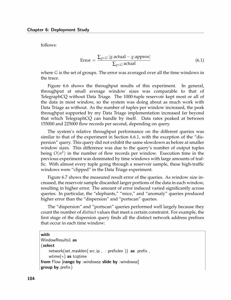
Chapter 6: Deployment Study
follows:
Error =∑g∈G |g.actual− g.approx|
∑g∈G actual(6.1)
where G is the set of groups. The error was averaged over all the time windows inthe trace.
Figure 6.6 shows the throughput results of this experiment. In general,throughput at small average window sizes was comparable to that ofTelegraphCQ without Data Triage. The 1000-tuple reservoir kept most or all ofthe data in most window, so the system was doing about as much work withData Triage as without. As the number of tuples per window increased, the peakthroughput supported by my Data Triage implementation increased far beyondthat which TelegraphCQ can handle by itself. Data rates peaked at between155000 and 225000 flow records per second, depending on query.
The system’s relative throughput performance on the different queries wassimilar to that of the experiment in Section 6.6.1, with the exception of the “dis-persion” query. This query did not exhibit the same slowdown as before at smallerwindow sizes. This difference was due to the query’s number of output tuplesbeing O(n2) in the number of flow records per window. Execution time in theprevious experiment was dominated by time windows with large amounts of traf-fic. With almost every tuple going through a reservoir sample, these high-trafficwindows were “clipped” in the Data Triage experiment.
Figure 6.7 shows the measured result error of the queries. As window size in-creased, the reservoir sample discarded larger portions of the data in each window,resulting in higher error. The amount of error induced varied significantly acrossqueries. In particular, the “elephants,” “mice,” and “anomaly” queries producedhigher error than the “dispersion” and “portscan” queries.
The “dispersion” and “portscan” queries performed well largely because theycount the number of distinct values that meet a certain constraint. For example, thefirst stage of the dispersion query finds all the distinct network address prefixesthat occur in each time window:
withWindowResults1 as(select
network(set masklen( src ip , : prefixlen )) as prefix ,wtime(∗) as tcqtime
from Flow [range by :windowsz slide by :windowsz]group by prefix)
104

6.6 Experiments
0
10
20
30
40
50
60
70
10 100 1000 10000 100000
Wei
ghte
d P
erce
nt E
rror
Avg Tuples/Window(log scale)
anomalydispersionelephants
miceportscans
Figure 6.7: Result error of TelegraphCQ with Data Triage, running my queries with vary-ing window sizes over the 5th week of the NERSC trace.
...
Due to the projection and duplicate elimination operations performed and theheavy-tailed distribution of our network traffic across prefixes, such queries canbe approximated from a small random sample of the input stream with relativelyhigh accuracy [47].
The remaining three queries produced higher result error. Analyzing the ap-proximate results of these queries in detail, I determined that these larger errorswere due to a combination of query and data characteristics. All three high-errorqueries computed SUM aggregates over the bytes sent field of the flow records.When using a random sample to approximate such an aggregate, the expected rel-ative error for the sum of a group is given by:
√(1− f )σ2 N
f
actual sum(6.2)
105

Chapter 6: Deployment Study
100
1000
10000
100000
1e+06
1e+07
1e+08
100 101 102 103 104 105 106 107 108 109
Coun
t (LO
G S
CALE
)
Bytes Sent (LOG SCALE)
Values of BYTES SENT Field
Figure 6.8: A histogram of observed values in the bytes sent field of the flow records inour trace. Note the logarithmic scale on both axes. The high variance of these valuesmakes it difficult to approximate queries that aggregate over this field.
where N is the number of tuples in the group, f is the fraction of tuples that areincluded in the sample, and and σ is the variance of the values in the group [39].
As Figure 6.8 shows, the values of the bytes sent field have extremely highvariance. Since the approximation error for a SUM aggregate is proportional to thevariance of the aggregate column, random sampling produced significant errorson the queries that computed SUM aggregates over the bytes sent column.
To demonstrate that the error I observed was in fact largely due to computingsums of a high-variance column, I replaced the SUM aggregates in the elephants,mice, and anomaly queries with COUNT aggregates and reran the experiment. AsFigure 6.9 shows, this change decreased the error of the elephants and mice queriessignificantly.
Error for the anomaly detection query also decreased with the switch to aCOUNT aggregate, but by a smaller factor. Since it computes a complete traf-fic matrix, the anomaly detection query produces results with a large number ofgroups. The random sample is spread across the groups, so the effective sample
106
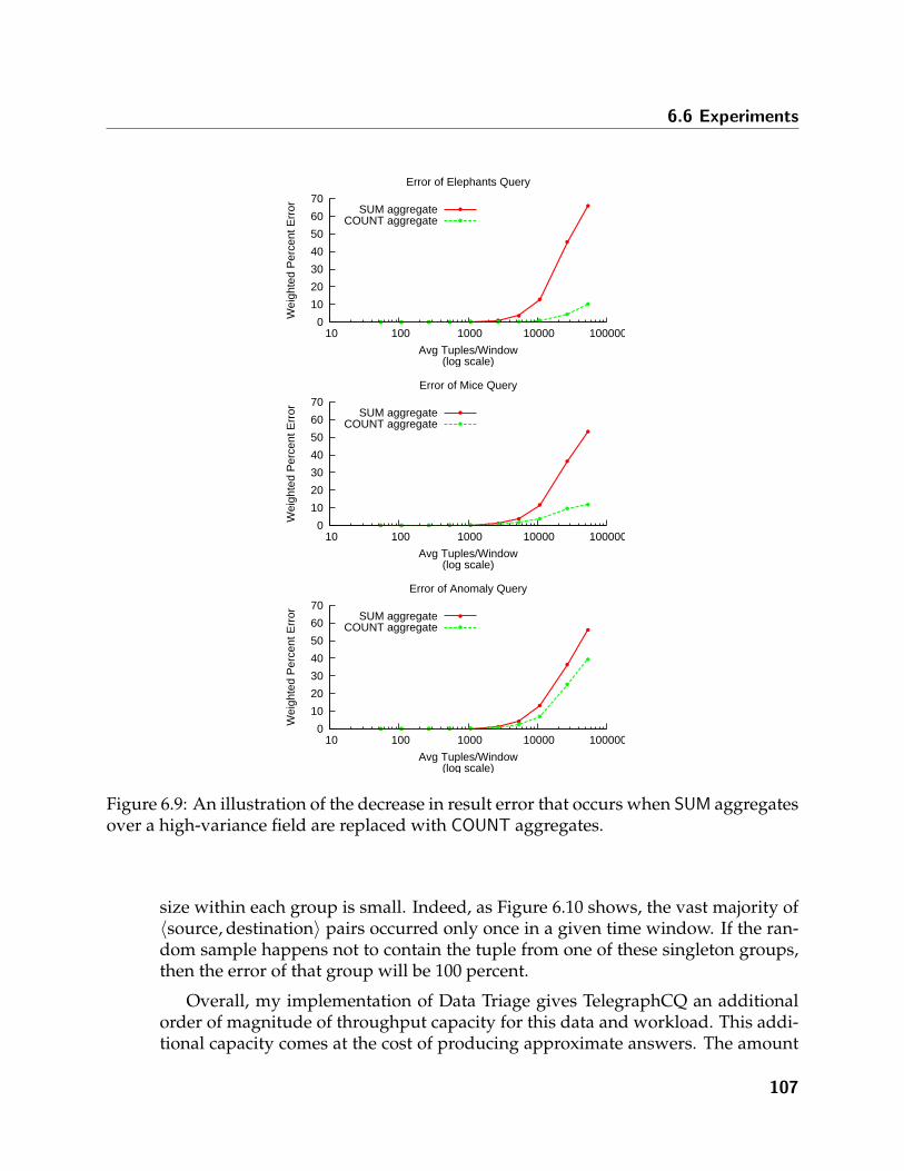
6.6 Experiments
0
10
20
30
40
50
60
70
10 100 1000 10000 100000
Wei
ghte
d P
erce
nt E
rror
Avg Tuples/Window(log scale)
Error of Elephants Query
SUM aggregateCOUNT aggregate
0
10
20
30
40
50
60
70
10 100 1000 10000 100000
Wei
ghte
d P
erce
nt E
rror
Avg Tuples/Window(log scale)
Error of Mice Query
SUM aggregateCOUNT aggregate
0
10
20
30
40
50
60
70
10 100 1000 10000 100000
Wei
ghte
d P
erce
nt E
rror
Avg Tuples/Window(log scale)
Error of Anomaly Query
SUM aggregateCOUNT aggregate
Figure 6.9: An illustration of the decrease in result error that occurs when SUM aggregatesover a high-variance field are replaced with COUNT aggregates.
size within each group is small. Indeed, as Figure 6.10 shows, the vast majority of〈source, destination〉 pairs occurred only once in a given time window. If the ran-dom sample happens not to contain the tuple from one of these singleton groups,then the error of that group will be 100 percent.
Overall, my implementation of Data Triage gives TelegraphCQ an additionalorder of magnitude of throughput capacity for this data and workload. This addi-tional capacity comes at the cost of producing approximate answers. The amount
107

Chapter 6: Deployment Study
0
1e+06
2e+06
3e+06
4e+06
5e+06
6e+06
7e+06
8e+06
100 80 60 40 20
Cou
nt
Number of Tuples in Group
>100
Figure 6.10: Histogram of the number of tuples in a group in the output of the “anomalydetection” query. A count of k means that a particular 〈source, destination〉 address pairappeared k times in a time window. The bins of the histogram for more than 10 tuples arehidden below the border of the graph.
of approximation error observed varies depending on the query, the data distri-bution, and the strengths of the particular approximation technique in use. Someparts of the query and data workload pushed the reservoir sampling techniquebeyond its useful range. Other approximation techniques may be able to correctfor this deficiency. In general, when using query approximation, it is importantto match the approximation technique to the expected query and data character-istics. Early observations of this fact motivated my design choice to modularizeData Triage’s approximation code.
6.6.3 FastBit
The next set of experiments measured the throughput of the FastBit componentof the system. I designed these experiments and worked with the FastBit team toimplement them. The experiments analyze FastBit’s performance in two separatecomponents: loading the index and querying the index. To measure index loadperformance, we conducted an experiment to determine the effect of batch size on
108

6.6 Experiments
1000
10000
100000
1e+06
100 1000 10000 100000 1e+06 1e+07 1e+08
Tu
ple
s p
er
se
co
nd
(lo
g s
ca
le)
Batch Size(log scale)
Figure 6.11: Speed for appending data and building the bitmap index in batches of sizesranging from 1,000 to 100,000,000. Each tuple contains 11 attributes (48 bytes).
load throughput. For querying performance, we measured average response timewhile varying the amount of historical data incorporated into the analysis.
6.6.3.1 Index Creation
We first measured the speed for appending new data and building the respec-tive bitmap indices. For these experiments we appended the data and built theindices in batches of various sizes to identify the most efficient batch size. In par-ticular, the batch sizes ranged from 1,000 to 100,000,000 tuples. Each tuple contains11 attributes.
Figure 6.11 shows the speed for building the bitmap indices in terms of tuplesper second. In our test data, each tuple is 48 bytes, 10 4-byte values plus 1 8-byte value. The maximum speed of 213,092 tuples per second is achieved whenthe append and index build operations are done in batches of 10,000,000 tuples.The performance graph also shows that the tuple rate decreases for batch sizesabove 10,000,000 tuples and later stays about constant at around 170,000 tuplesper second.
109

Chapter 6: Deployment Study
When the batch size is small, say, 1000 tuples, fixed overheads such as openingindex scans and parsing schema information dominate the overall running time.When the batch size is in the millions, the total time required to load the indexis dominated by the overhead of constructing index records and writing them todisk.
Once the batch size increases beyond 10 million records, throughput decreasessomewhat due to caching effects. To enable query processing during index buildoperations, FastBit keeps two copies of the index. These copies are stored in indexdirectories called the active directory and backup directory. During a bulk load oper-ation, the system first loads new tuples into the backup directory. Once the backupdirectory is up to date, FastBit swaps the active and backup directories and copiesthe new index records to the former active directory. When the batch size sur-passes 10 million records, the newly-created records no longer fit in the operatingsystem’s buffer cache, so the final bulk copy operation must read data from diskinstead of memory.
6.6.3.2 Index Lookup
In the following experiments we measure the throughput of the index lookups(query response time) of the five queries described in Section 5. Apart from the“mice” queries (see Section 5.2), the starting point for all the queries was one day’sworth of output data produced by TelegraphCQ. In particular, the TelegraphCQcontinuous queries as described in Section 5 were run starting from week 5. Next,the output of these queries was used as input for FastBit to query the historicaldata. In order to measure the scalability of FastBit, we varied the length of historybetween 1 and 28 days. All queries were executed with 10 different lengths of his-tory of equal size in the range of 1 and 28 days. By increasing the length of history,the result set (number of records fetched) of the queries increases monotonicallyand thus allows us to measure the query response time as a function of the resultsize.
Figure 6.12 shows the average query response time for all the 5 query typeswith 10 different lengths of history. In total, 100 × 10 queries were executed perquery type on 100 million tuples with different lengths of history. The input for the100 queries was randomly selected from the output of the TelegraphCQ stream-ing queries. In general, we observe a linear query response time with respect tothe number of records fetched. One can see that the “elephants” and “portscans”queries have the best query response times between 0.1 and 1 seconds. The “mice”,“anomalies” and “dispersion” queries have a higher query response time sincethey fetch more records. In fact, for large historical window sizes, nearly all of the100 million records are fetched. Thus, the query response time is dominated by thetime spent on fetching the results as opposed to the time spent on evaluating thequeries with the bitmap index. For example, it takes about 20 seconds to answer
110

6.6 Experiments
0.01
0.1
10
1
100
1000 10000 100000 1e+06 1e+07 1e+08
Ave
rag
e Q
ue
ry R
un
tim
e (
se
c)
(lo
g s
ca
le)
Number of Records Fetched(log scale)
anomaliesdispersionelephants
miceportscans
Figure 6.12: FastBit index lookup time for 5 types of historical queries with variouslengths of history denoted by variable : history .
the “anomalies” and “mice” queries when they fetch about 100 million records.Since both these queries select two attributes of 4-byte each, a total of about 800MB are read into memory and sorted to compute aggregate functions. This leadsto a reading speed of about 40 MB/s, which is nearly optimal because the readoperations are not contiguous (some records are not needed). This implies thatthe time spent in evaluating the range conditions in these queries over 100 millionrecords were negligible. The total query processing time is dominated by readingthe selected values.
6.6.4 Controller
Overall, the Controller component was not a bottleneck. I measured Controlleroverhead by running the TelegraphCQ query select ∗ from Flow on TelegraphCQvia the Controller, while sending flow data directly to TelegraphCQ. This queryproduces an output tuple for every input tuple and therefore puts stress on theController. I found that the TelegraphCQ Front End process dominated CPU us-age. The rate at which the Controller can consume tuples was not a bottleneck. Forthe workload I studied in this chapter, the analysis and report generation functions
111
Chapter 6: Deployment Study
of the Controller consumed far less CPU time than the process of receiving andparsing result tuples from TelegraphCQ. This distribution of work may change inthe future if our system were to incorporate complex predictive logic such as thatproposed by Soule et al.[99]. Currently, however, the Controller component is nota bottleneck.
6.6.5 End-to-end Throughput Without Data Triage
My next two sets of experiments combined TelegraphCQ, the FastBit loader,the FastBit query engine, the Controller, and the Ingress Manager to create an end-to-end system. For the first round of experiments, I disabled the Data Triage com-ponents of the Ingress Manager. I fed our trace through this system and measuredthe time until the Controller produced its last report. I then used this total elapsedtime and the number of tuples in the trace to compute the number of flow recordsper second that the system can consume without Data Triage.
I benchmarked each pair of TelegraphCQ/FastBit queries separately. Theranges of time selected in the FastBit queries were as depicted in Section 6.5.I varied the window size of the TelegraphCQ queries over the range of timeintervals used in Section 6.6.1. Flow records were appended to the FastBit indexin batches of 1 million.
Figure 6.13 shows the results of this experiment. Each thick line shows theperformance of a TelegraphCQ/FastBit query pair. The thin dotted line indicatesthe number of flow records per second the system would need to sustain to be ableto deliver results at 1-second intervals. Points above this threshold indicate datarates at which the system can support window sizes of 1 second.
At smaller window sizes, FastBit lookup time dominated the combined queryprocessing time. As window size increased, TelegraphCQ’s performance came todominate the system throughput. One exception to this rule was the mice querieswhere the FastBit component is executed offline prior to starting the TelegraphCQcomponent. Since the system loaded tuples in large batches and ran the FastBitappend operations and querying operations sequentially, the time spent on ap-pending 1 million flow records (about 4 seconds) caused a temporary lag in thequery response time. However, the decrease in overall throughput due to loadingthe index was negligible.
While most of the other queries produced similar throughput curves, the dis-persion query showed an especially high degree of performance variation at dif-ferent window sizes. Throughput for the dispersion queries did not reach com-parable levels to that of the other queries until the number of tuples per windowapproached 20,000. This delayed increase was due to three factors. As I observedin the previous section, the TelegraphCQ component of the queries runs slowlyat smaller window sizes. Also, the FastBit query for this analysis is also slower
112

6.6 Experiments
10
100
1000
10000
100000
10 100 1000 10000 100000
Flo
w R
ecord
s/s
ec
(log s
cale
)
Average Number of Records per Window(log scale)
anomalydispersionelephants
miceportscans
Min. for 1-second windows
Figure 6.13: End-to-end throughput with varying window sizes over the 5th week of theNERSC trace. Note the logarithmic scale. The thin dotted line indicates the minimumthroughput necessary to deliver results at 1-second intervals.
since the amount of data fetched is very large. Finally, as I noted in Section 6.5, thecurrent version of the query returns traffic broken down by address instead of bysubnet. As a workaround, the Controller currently reads in the (much expanded)results of the FastBit query and performs an additional round of aggregation bysubnet. The FastBit team is working to remove this bottleneck by adding supportfor arithmetic expressions in FastBit’s select lists.
In Figure 6.13 I also show the minimum performance needed to support a timewindow of 1 second. In this application, a window size of 1 second is extremelyshort. Even in this case, the system can handle between 9,000 and 20,000 flowrecords per second when running a single analysis on our test machine. Such datarates are in line with my estimates (See Section 6.2.1) of the average combineddata rates for all DOE labs. However, the system tested in this experiment cannothandle my estimated peak rates of 1.6 million records per second. To handle thesebursts of data, the system could either spool flow records to disk for later pro-cessing, use Data Triage [87] to trade off query result accuracy for response time,or add additional CPU capacity (possibly via parallelism [95]) to the system. The
113

Chapter 6: Deployment Study
10
100
1000
10000
100000
10 100 1000 10000 100000
Tupl
es/s
ec(lo
g sc
ale)
Average Number of Tuples per Window(log scale)
anomalydispersionelephants
miceportscans
Min. for 1-second windows
Figure 6.14: End-to-end throughput at varying window sizes with Data Triage enabled.Note the logarithmic scale. The thin dotted line indicates the minimum throughput nec-essary to deliver results at 1-second intervals.
experiments in Section 6.6.7 explore the tradeoffs between these three approaches.
6.6.6 End-to-end Throughput With Data Triage
My next experiment was similar in overall structure to the experiment in theprevious section, except that it measured throughput with Data Triage. As be-fore, the experiment used the end-to-end system, including index loading and bothTelegraphCQ and FastBit queries. For this second experiment, I also enabled theData Triage components in the Ingress Manager. Figure 6.14 shows the results ofthis experiment. Throughput is limited by FastBit query performance when thenumber of tuples per window is small. As the number of tuples per window in-creases, throughput goes up, eventually reaching a plateau of roughly 60000 tuplesper second for all of the queries. This plateau is due primarily to the speed withwhich the system could stage tuples to disk and load them into FastBit. The flowrecords start as a single stream of comma-delimited text, and the FastBit loaderexpects a separate binary file for each column. Conversion of text to binary andthe writing of multiple binary files consumes approximately as much CPU time as
114

6.6 Experiments
the actual index load operation, limiting overall throughput.
Since the TelegraphCQ components of the system had not changed from thoseused in Section 6.6.2, result accuracy in estimating the results of the TelegraphCQqueries was the same as before. Approximation was not used for the FastBit por-tion of the queries.
In practice, index loading should not have a serious effect on the system’s abil-ity to absorb bursts without delaying query results. In the query workload I usedin this study (See Section 6.5, the historical data that is used for comparison withcurrent trends is always at least 24 hours in the past. Strong diurnal and weeklypatterns in network traffic make it unnatural to compare current trends againsttraffic from a different time of day or day of the week. Because my queries do notneed data from the most recent 24 hours of history, the system is free to defer in-dex loading for up to 24 hours if a sustained burst of traffic exceeds its indexingcapacity. This deferred-loading strategy is similar to that used by Chandrasekaranand Franklin in their work on indexing archived streams [20].
Deferring indexing gives the system significant additional “headroom” to con-sume data during such bursts, as Figure 6.15 shows. The graph in Figure 6.15 illus-trates query throughput when indexing operations are (temporarily) disabled. Asthe graph illustrates, the end-to-end system can sustain bursts in excess of 200000flow records per second as long as the system can defer index loading until a rela-tively quiet period in the future.
6.6.7 Timing-Accurate Playback and Latency
My next set of experiments measured the end-to-end latency of query resultsover time. I wrote a program that plays back the trace at a multiple of real time, us-ing the timestamps embedded in the trace to determine when to send flow recordsto the system. I ran this program on the trace used in the previous sections’ exper-iments, selecting speed multiples such that the average data rate was from 50 to200 percent of the system’s measured throughput capability from the experimentsin Section 6.6.5. I measured the delay of query results by comparing the time at theend of the window with the time at which the system produced the window’s re-port for the user. I repeated the experiment both with the Data Triage componentsof the system both enabled and disabled.
Figures 6.16 through 6.20 show the results of the experiments. Overall, whenthe average data rate was 50% of the system’s capacity, the system was generallyable to return results with a delay of less than 10-15 seconds, with or without DataTriage. However, when the average rate of data arrival was equal to the system’scapacity, the no-triage runs of the experiment built up a persistent delay that onlygradually decreased during periods of relatively light traffic. In contrast, with Data
115

Chapter 6: Deployment Study
1000
10000
100000
1e+06
100 1000 10000 100000 1e+06
Tupl
es/s
ec(lo
g sc
ale)
Average Number of Tuples per Window(log scale)
anomalydispersionelephants
miceportscans
Figure 6.15: End-to-end throughput at varying window sizes with Data Triage enabledand index loading disabled. Note the logarithmic scale.
Triage enabled, delay remained consistently below 10 seconds.
At 200% of capacity, query result delay increases continually without DataTriage. After ten minutes of traffic at this rate, the no-triage runs of the experimentwere 5-10 minutes behind real time. Such a delay would be highly detrimentalto the efforts of administrators to find the cause of the surge in bandwidth usage.With Data Triage enabled, however, delay remained below 10 seconds as before.
Delay when running the “dispersion” query followed the same general trendas that of the other runs. However, the result delay with Data Triage enabled occa-sionally reached as high as 20 seconds before dropping back below the 10-seconddelay constraint. The current version of TelegraphCQ delays most of the process-ing for each time window until the end of the window. Also, the query’s innermostsubquery specified a 100-second time window that advances at 10-second inter-vals. The current version of TelegraphCQ recomputes query results for the entirewindow each time it advances, which in this case increases the amount of workfor this subquery by a factor of 10. These factors create a significant delay betweenthe time a tuple enters TelegraphCQ and the time that processing triggered by the
116

6.6 Experiments
0 2 4 6 8
10 12 14 16
0 200 400 600 800 1000 1200 1400 1600 1800
Que
ry R
esul
t Del
ay (s
ec)
Offset into Trace (sec)
Query result delay for elephants query(Average rate 50% of capacity)
No TriageTriage
0 10 20 30 40 50 60
0 100 200 300 400 500 600 700 800 900
Que
ry R
esul
t Del
ay (s
ec)
Offset into Trace (sec)
Query result delay for elephants query(Average rate 100% of capacity)
No TriageTriage
0 50
100 150 200 250 300 350
0 50 100 150 200 250 300 350 400 450
Que
ry R
esul
t Del
ay (s
ec)
Offset into Trace (sec)
Query result delay for elephants query(Average rate 200% of capacity)
No TriageTriage
Figure 6.16: Measured query result latency over time for the “elephants” query. In thefirst graph, the system was running at 50% of average capacity. The second graph shows100% capacity, and the third graph shows 200% capacity.
117

Chapter 6: Deployment Study
0
5
10
15
20
25
0 500 1000 1500 2000 2500
Que
ry R
esul
t Del
ay (s
ec)
Offset into Trace (sec)
Query result delay for mice query(Average rate 50% of capacity)
No TriageTriage
0 20 40 60 80
100 120 140 160 180
0 200 400 600 800 1000 1200
Que
ry R
esul
t Del
ay (s
ec)
Offset into Trace (sec)
Query result delay for mice query(Average rate 100% of capacity)
No TriageTriage
0 100 200 300 400 500 600 700
0 100 200 300 400 500 600
Que
ry R
esul
t Del
ay (s
ec)
Offset into Trace (sec)
Query result delay for mice query(Average rate 200% of capacity)
No TriageTriage
Figure 6.17: Measured query result latency over time for the “mice” query. In the firstgraph, the system was running at 50% of average capacity. The second graph shows100% capacity, and the third graph shows 200% capacity.
118
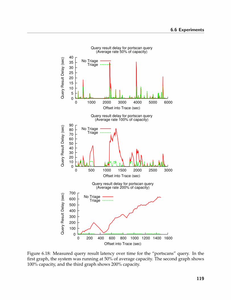
6.6 Experiments
0 5
10 15 20 25 30 35 40
0 1000 2000 3000 4000 5000 6000
Que
ry R
esul
t Del
ay (s
ec)
Offset into Trace (sec)
Query result delay for portscan query(Average rate 50% of capacity)
No TriageTriage
0 10 20 30 40 50 60 70 80 90
0 500 1000 1500 2000 2500 3000
Que
ry R
esul
t Del
ay (s
ec)
Offset into Trace (sec)
Query result delay for portscan query(Average rate 100% of capacity)
No TriageTriage
0 100 200 300 400 500 600 700
0 200 400 600 800 1000 1200 1400 1600
Que
ry R
esul
t Del
ay (s
ec)
Offset into Trace (sec)
Query result delay for portscan query(Average rate 200% of capacity)
No TriageTriage
Figure 6.18: Measured query result latency over time for the “portscans” query. In thefirst graph, the system was running at 50% of average capacity. The second graph shows100% capacity, and the third graph shows 200% capacity.
119

Chapter 6: Deployment Study
0 2 4 6 8
10 12 14 16
0 500 1000 1500 2000 2500
Que
ry R
esul
t Del
ay (s
ec)
Offset into Trace (sec)
Query result delay for anomaly query(Average rate 50% of capacity)
No TriageTriage
0 10 20 30 40 50 60 70
0 200 400 600 800 1000 1200
Que
ry R
esul
t Del
ay (s
ec)
Offset into Trace (sec)
Query result delay for anomaly query(Average rate 100% of capacity)
No TriageTriage
0 50
100 150 200 250 300 350 400 450
0 100 200 300 400 500 600
Que
ry R
esul
t Del
ay (s
ec)
Offset into Trace (sec)
Query result delay for anomaly query(Average rate 200% of capacity)
No TriageTriage
Figure 6.19: Measured query result latency over time for the “anomaly detection” query.In the first graph, the system was running at 50% of average capacity. The second graphshows 100% capacity, and the third graph shows 200% capacity.
120

6.6 Experiments
0
5
10
15
20
25
0 200 400 600 800 1000 1200 1400 1600
Que
ry R
esul
t Del
ay (s
ec)
Offset into Trace (sec)
Query result delay for disp query(Average rate 50% of capacity)
No TriageTriage
0 10 20 30 40 50 60 70
0 100 200 300 400 500 600 700
Que
ry R
esul
t Del
ay (s
ec)
Offset into Trace (sec)
Query result delay for disp query(Average rate 100% of capacity)
No TriageTriage
0 50
100 150 200 250 300
0 50 100 150 200 250 300
Que
ry R
esul
t Del
ay (s
ec)
Offset into Trace (sec)
Query result delay for disp query(Average rate 200% of capacity)
No TriageTriage
Figure 6.20: Measured query result latency over time for the “dispersion” query. In thefirst graph, the system was running at 50% of average capacity. The second graph shows100% capacity, and the third graph shows 200% capacity.
121

Chapter 6: Deployment Study
tuple is completed. As a result, when the Triage Scheduler begins triaging tuples,TelegraphCQ has already buffered a large number of tuples internally, leading toa delay before response time begins to improve.
Developers on the commercial version of TelegraphCQ are currently makingimprovements that should greatly reduce this internal delay. In particular, thesedevelopers are implementing a hash-based GROUP BY to avoid buffering an entirewindow’s results, as well as efficient methods of incrementally computing queryresults when the RANGE of a window clause is greater than its SLIDE.
6.6.8 Measuring the Latency-Accuracy Tradeoff
My final experiment measured the effect of the user’s choice of delay constrainton query result accuracy. For this experiment, I used the setup from the previoussection’s experiments. First, I ran the TelegraphCQ components of the querieswithout Data Triage and logged the full query answers to disk. Then I enabled allcomponents of the system, including the Data Triage and indexing components,and reran the trace at a 100% average load, logging the results of the main andshadow queries to disk. I repeated the experiment while varying the delay con-straint from 2 seconds to 100 seconds. Afterwards, a postprocessing step measuredquery result error using the same technique used in Section 6.6.2.
Figure 6.21 shows the results of this experiment. All five queries behaved sim-ilarly as the delay constraint varied, with error decreasing as the number of tuplesthe system needed to triage went down. Interestingly, the relative amounts of erroracross the queries differed compared with the results in Section 6.6.2.
Whereas the earlier experiment forced the system to triage every tuple, the ex-periment in this section “played back” the trace at a multiple of real time, allowingthe Triage Scheduler to choose which tuples to triage. In this real-time experiment,the queries consumed data at different rates, and these rates varied depending onthe characteristics of the data itself. For example, when there were many combi-nations of address and port in a given time window, the “portscans” query, whichcomputes the set of unique 〈address, port〉 combinations, slowed down by a largerdegree than the other queries. Overall, the errors across queries were closer to-gether in the real-time experiment, indicating that the timing of triage decisionscan be as important to query result error as the quality of the query approximationitself.
122

6.7 Conclusions
6.7 ConclusionsThe results in this chapter demonstrate that an end-to-end system that uses
Data Triage for monitoring high-speed networking data streams is feasible. Theyalso show that my extension Data Triage to support archival is a viable architec-ture. I demonstrated that, without Data Triage, a network monitoring system canbottleneck on the streaming query processor, causing significant delays in queryresult generation. I I found that overprovisioning the monitoring hardware by afactor of 2 to 4 would keep query result latency below a 10-second threshold. WithData Triage enabled, query result latency would stay under control, using signifi-cantly less hardware than would be necessary to achieve the same latency withoutData Triage.
123

Chapter 6: Deployment Study
0
2
4
6
8
10
12
14
16
1 10 100 1000
Wei
ghte
d P
erce
nt E
rror
Delay Constraint (sec)(log scale)
anomalydispersionelephants
miceportscans
Figure 6.21: Error of query results with Data Triage as the delay constraint varies. Theaverage data rate was 100% of TelegraphCQ’s capacity. Each point represents the meanof 5 runs of the experiment; error bars indicate standard deviation.
124

Chapter 7
Conclusion
People do not like to think. If one thinks, one must reach conclusions. Conclusions arenot always pleasant.
— Helen Keller (1880 - 1968)
125

Chapter 7: Conclusion
Enterprise networks have been increasing in complexity while at the same timebecoming more vital to the operations of global organizations. These trends createa need for network monitoring systems that run declarative queries and can ob-serve the low level traffic on each network link. Unfortunately, passive networkmonitoring currently requires a significant amount of processing power to keepup with the maximum data rate of a network link, and hardware costs represent asignificant barrier to the adoption of such an infrastructure.
My approach to solving this hardware cost problem takes advantage of thebursty nature of network traffic by using hardware provisioned for the averagedata rate on the network link, which is generally at least an order of magnitudeless than the maximum rate. Of course, such a strategy requires a comprehensivestrategy for handling the overload that will inevitably occur when a burst of high-speed network traffic exceeds the system’s capacity.
In this dissertation, I have described the principle components of such a strat-egy:
• The Data Triage architecture, which adds a fallback mechanism based on ap-proximate query processing to a streaming query processor.
• The Delay Constraints API and associated scheduling algorithm, which con-trol the tradeoffs between query result delay and accuracy in the Data Triagearchitecture.
• New histogram-based query approximations that allow Data Triage’s approx-imate data path to cover an important class of network monitoring query be-yond those that existing techniques already support.
Finally, I described a deployment study that demonstrates that my Data Triageimplementation functions properly in the context of an end-to-end monitoring sys-tem being developed for the U.S. Department of Energy’s laboratory networks.
126

Bibliography[1] T.F. Abdelzaher, J.A. Stankovic, Chenyang Lu, Ronghua Zhang, and Ying Lu. Feed-
back performance control in software services. Control Systems Magazine, June 2003.1.3
[2] Swarup Acharya, Phillip B. Gibbons, and Viswanath Poosala. Congressional sam-ples for approximate answering of group-by queries. In SIGMOD, pages 487–498,2000. 2.2.1
[3] Swarup Acharya, Phillip B. Gibbons, Viswanath Poosala, and Sridhar Ramaswamy.Join synopses for approximate query answering. In SIGMOD, pages 275–286, 1999.2.2.1, 3.1.1
[4] AmberPoint. Closed-loop governance: Amberpoint solutions, 2006.http://www.amberpoint.com/solutions/governance.shtml. 1.3
[5] APNIC. Whois database, October 2005. ftp://ftp.apnic.net/apnic/whois-data/APNIC/apnic.RPSL.db.gz. 5.6
[6] A. Arasu, S. Babu, and J. Widom. The CQL continuous query language: Semanticfoundations and query execution. Technical Report 2003-67, Stanford University,2003. 1.6.1.1
[7] Internet Assigned Numbers Authority. http://www.iana.org. 5.2
[8] Raian Babcock, Surajit Chaurhuri, and Gautam Das. Dynamic sample selection forapproximate query processing. In SIGMOD, 2003. 2.2.1
[9] J.C.R. Bennett and Hui Zhang. WF2Q: Worst-case fair weighted fair queueing. InINFOCOM, volume 1, pages 120–128, 1996. 2.3
[10] J.L. Bentley. Multidimensional binary search trees used for associative searching.Communications of the ACM, pages 509–517, 1975. 4.7.1
[11] E. Wes Bethel, Scott Campbell, Eli Dart, Kurt Stockinger, and Kesheng Wu. Accel-erating Network Traffic Analysis Using Query-Driven Visualization. In 2006 IEEESymposium on Visual Analytics Science and Technology (to appear), 2006. 2.5, 6.2
127

BIBLIOGRAPHY
[12] Nicolas Bruno, Surajit Chaudhuri, and Luis Gravano. STHoles: a multidimensionalworkload-aware histogram. SIGMOD Record, 30(2):211–222, 2001. 2.4
[13] Shaofeng Bu, Laks V.S. Lakshmanan, and Raymond T. Ng. Mdl summarizationwith holes. In VLDB, 2005. 2.4
[14] A. Buchsbaum, G. Fowler, B. Krishnamurthy, K. Vo, and J. Wang. Fast prefix match-ing of bounded strings. In ALENEX, 2003. 2.4
[15] Ahmet Bulut and Ambuj K. Singh. Swat: Hierarchical stream summarization inlarge networks. In ICDE, 2003. 2.2.1
[16] W. Burlesona, J. Ko, D. Niehaus, K. Ramamritham, J.A. Stankovic, G. Wallace, andC. Weems. The spring scheduling coprocessor: a scheduling accelerator. Very LargeScale Integration (VLSI) Systems, IEEE Transactions on, 1999. 2.3
[17] Kaushik Chakrabarti, Minos Garofalakis, Rajeev Rastogi, and Kyuseok Shim. Ap-proximate query processing using wavelets. VLDB Journal, 10(2–3):199–223, 2001.2.2.1, 3.1.1
[18] C. Y. Chan and Y. E. Ioannidis. An Efficient Bitmap Encoding Scheme for SelectionQueries. In SIGMOD, 1999. 2.5
[19] S. Chandrasekaran, Owen Cooper, Amol Deshpande, Michael J. Franklin, Joseph M.Hellerstein, Wei Hong, Sailesh Krishnamurthy, Sam Madden, Vijayshankar Raman,Fred Reiss, and Mehul Shah. Telegraphcq: Continuous dataflow processing for anuncertain world. In CIDR, 2003. 1.6.1.1, 1.6.1.2
[20] Sirish Chandrasekaran and Michael Franklin. Remembrance of Streams Past:Overload-Sensitive Management of Archived Streams. In VLDB, 2004. 2.5, 3.4,6.6.6
[21] S. Chaudhuri, R. Motwani, and V.R. Narasayya. On random sampling over joins.In SIGMOD, 1999. 2.2.1
[22] B-C. Chen, V. Yegneswaran, P. Barford, and R. Ramakrishnan. Toward a QueryLanguage for Network Attack Data. In NetDB Workshop, 2006. 2.5, 6.5.5
[23] AT&T Corp. Making the case for enterprise mobility. Technical Report AB-0421-01,AT&T, May 2006. 1.2
[24] Charles D. Cranor, Theodore Johnson, Oliver Spatscheck, and VladislavShkapenyuk. Gigascope: A stream database for network applications. In SIGMOD,2003. 2.2
[25] Chuck Cranor, Yuan Gao, Theodore Johnson, Vlaidslav Shkapenyuk, and OliverSpatscheck. Gigascope: high performance network monitoring with an sql inter-face. In SIGMOD, 2002. 1.4, 2.2
128
BIBLIOGRAPHY
[26] Roger O. Crockett. Ip’s killer apps are coming. BusinessWeek, March 2006. 1.2
[27] Abhinandan Das, J. E. Gehrke, and Mirek Riedewald. Approximate join processingover data streams. In SIGMOD. ACM Press, 2003. 2.2.1
[28] A. Demers, S. Keshav, and S. Shenker. Analysis and simulation of a fair queueingalgorithm. In SIGCOMM ’89: Symposium proceedings on Communications architectures& protocols, pages 1–12, New York, NY, USA, 1989. ACM Press. 2.3
[29] Amol Deshpande and Joseph Hellerstein. On using correlation-based synopsesduring query optimization. Technical Report CSD-02-1173, U.C. Berkeley EECSDepartment, May 2002. 2.4, 3.1.1
[30] Holger Dreger, Anja Feldmann, Vern Paxson, and Robin Sommer. Operational ex-periences with high-volume network intrusion detection. In CCS, pages 2–11. ACMPress, 2004. 2.2
[31] eMarketer. Online ad spending still growing in the us and uk. eMarketer.com, June2006. 1.2
[32] Pl Erik Eng and Morten Haug. Automatic response to intrusion detection. Master’sthesis, Agder University College, Grimstad, June 2004. 1.3
[33] Rajeev Motwani et al. Query processing, resource management, and approximationin a data stream management system. In CIDR. ACM Press, 2003. 2.2.1
[34] Information Technology for European Advancement. The explosive growth ofservice-oriented architecture adoption. Technical report, ITEA, 2005. 1.2
[35] V. Fuller, T. Li, J. Yu, and K. Varadhan. RFC 1519: Classless inter-domain rout-ing (CIDR): an address assignment and aggregation strategy, September 1993.ftp://ftp.internic.net/rfc/rfc1519.txt. 2.4, 5.2
[36] Minos Garofalakis and Phillip Gibbons. Approximate query processing: Tamingthe terabytes!, 2001. 2.2.1
[37] Minos Garofalakis and Amit Kumar. Deterministic wavelet thresholding formaximum-error metrics. In PODS, 2004. 2.4, 5.3.2.3
[38] Lise Getoor, Benjamin Taskar, and Daphne Koller. Selectivity estimation using prob-abilistic models. In SIGMOD Conference, 2001. 2.2.1
[39] Larry Gonick and Woollcott Smith. The Cartoon Guide to Statistics. HarperPerennial,1993. 6.6.2
[40] Goetz Graefe. Goetz graefe. SIGMOD Record, 18(9):509–516, 2006. 2.5
129

BIBLIOGRAPHY
[41] Jim Gray, Surajit Chaudhuri, Adam Bosworth, Andrew Layman, Don Reichart, Mu-rali Venkatrao, Frank Pellow, and Hamid Pirahesh. Data cube: A relational aggre-gation operator generalizing group-by, cross-tab, and sub-totals. J. Data Mining andKnowledge Discovery, 1(1):29–53, 1997. 5.3.2.3
[42] Aberdeen Group. Hosted crm gains momentum as salesforce.com paces the market.Technical report, Aberdeen Group, October 2003. 1.2
[43] Sudipto Guha. Space efficiency in synopsis construction algorithms. In VLDB, 2005.5.5.4
[44] Sudipto Guha, Nick Koudas, and Divesh Srivastava. Fast algorithms for hierarchi-cal range histogram construction. In PODS, 2002. 2.4
[45] Ashish Gupta and Inderpal Singh Mumick. Maintenance of materialized views:Problems, techniques, and applications. IEEE Data Eng. Bull., 18(2):3–18, 1995. 3.3.2
[46] Peter J. Haas and Joseph M. Hellerstein. Ripple joins for online aggregation. InAlex Delis, Christos Faloutsos, and Shahram Ghandeharizadeh, editors, SIGMOD,pages 287–298. ACM Press, 1999. (document), 3.3.3, A.1
[47] Joseph M. Hellerstein, Peter J. Haas, and Helen J. Wang. Online aggregation. InSIGMOD, pages 171–182, 1997. 6.6.2
[48] Gianluca Iannaccone, Christophe Diot, and Derek McAuley. The CoMo white pa-per. Technical Report IRC-TR-04-017, Intel Research, September 2004. 2.2
[49] Yannis E. Ioannidis. Universality of serial histograms. In VLDB, pages 256–267, SanFrancisco, CA, USA, 1993. Morgan Kaufmann Publishers Inc. 2.4
[50] Yannis E. Ioannidis and Viswanath Poosala. Balancing histogram optimality andpracticality for query result size estimation. In SIGMOD, pages 233–244, New York,NY, USA, 1995. ACM Press. 2.4, 5.6
[51] H. V. Jagadish, Nick Koudas, S. Muthukrishnan, Viswanath Poosala, Kenneth C.Sevcik, and Torsten Suel. Optimal histograms with quality guarantees. In VLDB,pages 275–286, 24–27 1998. 2.4, 3.1.1
[52] H. V. Jagadish, Nick Koudas, S. Muthukrishnan, Viswanath Poosala, Kenneth C.Sevcik, and Torsten Suel. Optimal histograms with quality guarantees. In VLDB,pages 275–286, 1998. 5.6
[53] Jaewoo Kang, Jeffrey F. Naughton, and Stratis D. Viglas. Evaluating window joinsover unbounded streams. In ICDE, 2003. 2.2.1
[54] Panagiotis Karras and Nikos Mamoulis. One-pass wavelet synopses for maximum-error metrics. In VLDB, 2005. 2.4
130

BIBLIOGRAPHY
[55] Masayoshi Kobayashi, Tutomu Murase, and Atsushi Kuriyama. A longest prefixmatch search engine for multi-gigabit ip processing. In IEEE International Conferenceon Communications, 2000. 5.2
[56] Stefan Kornexl, Vern Paxson, Holger Dreger, Anja Feldmann, and Robin Sommer.Building a Time Machine for Efficient Recording and Retrieval of High-Volume Net-work Traffic. In Internet Measurement Conference, 2005. 2.5
[57] Nick Koudas, S. Muthukrishnan, and Divesh Srivastava. Optimal histograms forhierarchical range queries (extended abstract). In PODS, pages 196–204, 2000. 2.4
[58] Sailesh Krishnamurthy and Michael J. Franklin. Shared hierarchical aggregationover receptor streams. Technical Report UCB-CSD-05-1381, UC Berkeley, 2005. 4.5,4.5.1
[59] Sailesh Krishnamurthy, Chung Wu, and Michael J. Franklin. On-the-fly sharing forstreamed aggregation. In SIGMOD, 2006. 4.5.2
[60] Iosif Lazaridis and Sharad Mehrotra. Capturing sensor-generated time series withquality guarantees. In ICDE, 2003. 2.2.1
[61] Will E. Leland, Murad S. Taqq, Walter Willinger, and Daniel V. Wilson. On the self-similar nature of Ethernet traffic. In Deepinder P. Sidhu, editor, ACM SIGCOMM,pages 183–193, 1993. 1.4
[62] L. Lim, M. Wang, and J. S. Vitter. Sash: A self-adaptive histogram set for dynami-cally changing workloads. In VLDB, 2003. 2.2.1
[63] C. L. Liu and James W. Layland. Scheduling algorithms for multiprogramming ina hard-real-time environment. Journal of the ACM, 20(1):46–61, 1973. 2.3
[64] Chenyang Lu, John A. Stankovic, Gang Tao, and Sang H. Son. Design and evalua-tion of a feedback control edf scheduling algorithm. In RTSS ’99: Proceedings of the20th IEEE Real-Time Systems Symposium, page 56, Washington, DC, USA, 1999. IEEEComputer Society. 2.3
[65] Sam Madden, Mehul A. Shah, Joseph M. Hellerstein, and Vijayshankar Raman.Continuously adaptive continuous queries over streams. In SIGMOD Conference,2002. 1.6.1.2
[66] Y. Matias, J. S. Vitter, and M. Wang. Dynamic maintenance of wavelet-based his-tograms. In VLDB, 2000. 2.2.1, 2.4, 4.7
[67] Yossi Matias, Jeffrey Scott Vitter, and Min Wang. Wavelet-based histograms forselectivity estimation. In SIGMOD, pages 448–459, 1998. 2.2.1, 2.4, 3.1.1
131

BIBLIOGRAPHY
[68] Research In Motion. Blackberry for sales professionals. Technical report, RIM, 2006.1.2
[69] M. Muralikrishna and D. DeWitt. Equi-depth histograms for estimating selectivityfactors for multidimensional queries. In SIGMOD, pages 28–36, 1998. 2.4
[70] S. Muthukrishnan, Viswanath Poosala, and Torsten Suel. “On Rectangular Parti-tionings in Two Dimensions: Algorithms, Complexity, and Applications”. In ICDT,Jerusalem, Israel, January 1999. 5.4.2.5, 5.4.2.5
[71] S. Muthukrishnan, Viswanath Poosala, and Torsten Suel. On rectangular partition-ings in two dimensions: Algorithms, complexity, and applications. Lecture Notes inComputer Science, 1540:236–256, 1999. 5.5.2
[72] J. Nagle. On packet switches with infinite storage. Communications, IEEE Transac-tions on, 35(4):435–438, April 1987. 2.3
[73] Peter Newman, Greg Minshall, Tom Lyon, Larry Huston, and Ipsilon Networks Inc.Ip switching and gigabit routers. IEEE Communications Magazine, 1997. 2.4, 5.2
[74] F. Olken and D. Rotem. Random sampling from databases - a survey. In Statisticsand Computing (invited paper), pages 25–42, 1995. 2.2.1
[75] P. O’Neil and D. Quass. Improved Query Performance with Variant Indices. InSIGMOD, 1997. 2.5
[76] Dmitry Pavlov and Heikki Mannila. Beyond independence: Probilistic models forquery approximation on binary transaction data. 2.2.1
[77] Dmitry Pavlov and Padhraic Smyth. Probabilistic query models for transactiondata. In KDD, pages 164–173, 2001. 2.2.1
[78] Vern Paxson. Bro: A System for Detecting Network Intruders in Real-Time. InUSENIX Security Symposium, January 1998. 2.5
[79] Vern Paxson and Sally Floyd. Wide-area traffic: the failure of Poisson modeling.IEEE Trans. Networking, 3(3):226 – 224, 1995. 1.4
[80] T. Plagemann, V. Goebel, A. Bergamini, G. Tolu, G. Urvoy-Keller, and E. W. Biersack.Using Data Stream Management Systems for Traffic Analysis - A Case Study. InPassive and Active Measurements, 2004. 2.5
[81] Viswanath Poosala, Peter J. Haas, Yannis E. Ioannidis, and Eugene J. Shekita. Im-proved histograms for selectivity estimation of range predicates. In SIGMOD, pages294–305, 1996. 2.4, 5.3.2.2
132

BIBLIOGRAPHY
[82] Viswanath Poosala and Yannis E. Ioannidis. Selectivity estimation without the at-tribute value independence assumption. In The VLDB Journal, pages 486–495, 1997.2.4, 3.1.1, 3.2.1, 4.7
[83] Postgresql database system. http://www.postgresql.org. 1.6.1
[84] Raghu Ramakrishnan and Johannes Gehrke. Database Management Systems.McGraw-Hill, 2002. 1.6.1.1
[85] K. Ramamritham and J. Stankovic. Dynamic task scheduling in distributed hardreal-time systems. IEEE Software, 1, 1984. 2.3
[86] Ramaswamy Ramaswamy, Ning Weng, and Tilman Wolf. A network processorbased passive measurement node. In Proc. of Passive and Active Measurement Work-shop (PAM), pages 337–340, Boston, MA, March 2005. (Extended Abstract). 2.2
[87] Frederick Reiss and Joseph M. Hellerstein. Declarative Network Monitoring withan Underprovisioned Query Processor. In ICDE, 2006. 2.5, 6.6.5
[88] Y. Rekhter and T. Li. RFC 1771: A Border Gateway Protocol 4 (BGP-4), March 1995.http://www.ietf.org/rfc/rfc1771.txt. 5.2
[89] R.H. Riedi and W. Willinger. Self-similar Network Traffic and Performance Evaluation.Wiley, 2000. 1.4
[90] RIPE. Whois database, September 2005. ftp://ftp.ripe.net/ripe/dbase/ripe.db.gz.5.6
[91] Martin Roesch. Snort-Lightweight Intrusion Detection for Networks. In USENIXLISA, 1999. 2.5
[92] Martin Roesch. Snort - lightweight intrusion detection for networks. Technicalreport, snort.org, 2006. 2.2
[93] Doron Rotem, Kurt Stockinger, and Kesheng Wu. Optimizing Candidate CheckCosts for Bitmap Indices. In CIKM, 2005. 2.5
[94] David V. Schuehler and John Lockwood. TCP-Splitter: A TCP/IP flow monitor inreconfigurable hardware. In Hot Interconnects, pages 127–131, Stanford, CA, August2002. 1.4
[95] Mehul A. Shah, Joseph M. Hellerstein, and Eric Brewer. Highly Available, Fault-Tolerant, Parallel Dataflows. In SIGMOD, 2004. 6.6.5
[96] Arie Shoshani, Luis Bernardo, Henrik Nordberg, Doron Rotem, and Alex Sim. Mul-tidimensional Indexing and Query Coordination for Tertiary Storage Management.In SSDBM, July 1999. 6.3
133

BIBLIOGRAPHY
[97] M. Shreedhar and George Varghese. Efficient fair queueing using deficit round-robin. IEEE/ACM Trans. Netw., 4(3):375–385, 1996. 2.3
[98] M. Siekkinen, E. W. Biersack, V. Goebel, T. Plagemann, and G. Urvoy-Keller. In-TraBase: Integrated Traffic Analysis Based on a Database Management System. InWorkshop on End-to-End Monitoring Techniques and Services, May 2005. 2.5
[99] A. Soule, K. Salamatian, and N. Taft. Combining filtering and statistical methods foranomaly detection. In ACM/Sigcomm Internet Measurement Conference (IMC), 2005.6.5.4, 6.6.4
[100] Utkarsh Srivastava and Jennifer Widom. Memory-limited execution of windowedstream joins, 2004. 2.2.1
[101] K. Stockinger and K.Wu et al. Network Traffic Analysis With Query Driven Visual-ization - SC 2005 HPC Analytics Results. In Super Computing, 2005. 2.5, 6.2
[102] Ion Stoica, Scott Shenker, and Hui Zhang. Core-stateless fair queueing: achiev-ing approximately fair bandwidth allocations in high speed networks. SIGCOMMComput. Commun. Rev., 28(4):118–130, 1998. 2.3
[103] Yufei Tao, Jimeng Sun, and Dimitris Papadias. Selectivity estimation for predictivespatio-temporal queries. In ICDE, 2003. 2.4, 3.1.1
[104] Nesime Tatbul, Ugur Centintemel, Stan Zdonik, Mitch Cherniack, and MichaelStonebraker. Load shedding in a data stream manager. In VLDB, 2003. 2.2.1
[105] Ravikumar V.C. and Rabi N. Mahapatra. Tcam architecture for ip lookup usingprefix properties. IEEE Micro, 24(2):60–69, 2004. 5.2
[106] Jeffrey S. Vitter. Random sampling with a reservoir. ACM Trans. Math. Softw.,11(1):37–57, 1985. 3.1.1, 4.7
[107] Carl A. Waldspurger and William E. Weihl. Lottery scheduling: Flexibleproportional-share resource management. In Operating Systems Design and Imple-mentation, pages 1–11, 1994. 2.3
[108] Carl A. Waldspurger and William E. Weihl. Stride scheduling: Deterministicproportional- share resource management. Technical Report MIT/LCS/TM-528,MIT, 1995. 2.3
[109] M. Wang, J. S. Vitter, L. Lim, and S. Padmanabhan. Wavelet-based cost estimationfor spatial queries. In Proceedings of the SSTD conference, 2001. 2.2.1
[110] N. Weaver, S. Staniford, and V. Paxson. Very fast containment of scanning worms.In USENIX Security Symposium, 2004. 1.3, 4.2
134

BIBLIOGRAPHY
[111] Richard West and Karsten Schwan. Dynamic window-constrained scheduling formultimedia applications. In ICMCS, Vol. 2, pages 87–91, 1999. 2.3
[112] Wikipedia. Port scanner — wikipedia, the free encyclopedia, 2006. [Online; ac-cessed 21-October-2006]. 2
[113] Kesheng Wu, Ekow Otoo, and Arie Shoshani. A Performance Comparison ofBitmap Indices. In CIKM, 2001. 2.5
[114] Kesheng Wu, Ekow Otoo, and Arie Shoshani. On the Performance of Bitmap In-dices for High Cardinality Attributes. In VLDB, 2004. 2.5, 6.3
[115] Kesheng Wu, Ekow J. Otoo, and Arie Shoshani. An Efficient Compression SchemeFor Bitmap Indices. ACM Transactions on Database Systems, 31:1–38, 2006. 2.5, 6.3
135

136

Appendix A
Differential Relational Algebra
This appendix defines a set of differential operators that correspond to the relationalalgebra operators 〈σ , π ,×,−〉. The crux of these derivations is to capture the effects onrelational algebra expressions when tuples disappear from their base relations.
137

Appendix A: Differential Relational Algebra
A.1 SelectionI define the differential selection operator σ(Snoisy, S+, S−) ≡ (Rnoisy, R+, R−)based on the standard selection operator σ as follows:
σ(Snoisy, S+, S−) ≡ (σ(Snoisy),σ(S+),σ(S−)). (A.1)
Intuitively, the differential selection operator simply applies the conventionalselection operator to all three parts of the stream.
A.2 ProjectionThe definition of the differential projection operator is similar to that of the differ-ential selection operator:
π(Snoisy, S+, S−) ≡ (π(Snoisy), π(S+), π(S−)). (A.2)
A.2.1 Duplicate Elimination
It is important to note that the differential projection operator only works prop-erly for multisets. This is not a problem for most queries, as multiset semantics arethe default for both SQL and CQL. However, SELECT DISTINCT queries requirean additional layer of post-processing to remove duplicates. A query in the form:
select distinct <columns> from <streams> where <predicates>
must be converted into the following before the rewrites in the remainder of thischapter can be applied:
select distinctfrom (select <columns> from <streams> where <predicates>) as subquery
Then the inner subquery is rewritten, leaving the outer query to evaluate theDISTINCT clause At runtime, each copy of a tuple in the additive noise or noisy partsof the result “cancels out” a copy of the tuple in the subtractive noise component.
138

A.3 Cross Product
S
T
(S-S )
Snoisy
noisy noisy
Tnoisy
S-
T-
-
(T-T )-
S+
T+
S×T
S ×T
Figure A.1: Intuitive version of the differential cross product definition. The large squarerepresents the tuples in the cross-product of (S + S+) with (T + T+), borrowing a vi-sual metaphor from Ripple Join [46]. The smaller shaded square inside the large squarerepresents the cross product of the original relations S and T. The speckled square rep-resents the cross product of these two relations after the tuples in S− and T− are re-moved and the tuples in S+ and T− are added to S and T, respectively. The differen-tial cross product computes the difference between these two cross products. Note thatSnoisy − S+ = S− S−.
A.3 Cross ProductThe definition of the differential cross-product operator is more complicated thanthe previous two operators.
Since
Snoisy ≡ S + S+ − S− (A.3)
Tnoisy ≡ T + T+ − T−, (A.4)
139

Appendix A: Differential Relational Algebra
for any relations S and T:
S× T = Snoisy × Tnoisy
−(
S+ × T+ + S+ × (Tnoisy − T+) + (Snoisy − S+)× T+)
+(
S− × T− + S− × (Tnoisy − T+) + (Snoisy − S+)× T−))
.
Figure A.1 shows the intuition behind the above formula.
Accordingly, I define the differential cross product operator × as
(Snoisy, S+, S−)×(Tnoisy, T+, T−) ≡ (Rnoisy, R+, R−) (A.5)
where
Rnoisy = Snoisy × Tnoisy
andR+ = S+ × T+ + S+ × (Tnoisy − T+) + (Snoisy − S+)× T+
andR− = S− × T− + S− × (Tnoisy − T+) + (Snoisy − S+)× T−).
140

A.4 Join
A.4 JoinThe relational join operator is the composition of cross-product and selection. Sim-ilarly, the differential join operator can be derived from the differential selectionand cross-product operators:
(Snoisy, S+, S−)./(Tnoisy, T+, T−) ≡ σ((Snoisy, S+, S−)×(Tnoisy, T+, T−)
)(A.6)
Substituting in the definitions of the differential selection and cross-productoperators produces the following definition:
(Snoisy, S+, S−)./(Tnoisy, T+, T−) ≡ (Rnoisy, R+, R−) (A.7)
where
Rnoisy = Snoisy ./ Tnoisy
andR+ = S+ ./ T+ + S+ ./ (Tnoisy − T+) + (Snoisy − S+) ./ T+
andR− = S− ./ T− + S− ./ (Tnoisy − T+) + (Snoisy − S+) ./ T−).
141

Appendix A: Differential Relational Algebra
S-T-
T+S+
noisy noisyTT
SS-
S-T-
T+
S+
noisy noisyTnoisyT
SnoisyS -
Figure A.2: Intuitive version of the definition of the differential set difference operator,(Snoisy, S+, S−)−(Tnoisy, T+, T−). This operator computes a delta between (Snoisy − Tnoisy)and (S− T), where Snoisy represents the tuples that remain in S after the query processordrops some of its input tuples. The shaded area in the Venn Diagram on the left containsthe tuples in (Snoisy − Tnoisy), and the shaded area in the diagram on the right containsthe tuples in (S − T). The shaded regions outlined in bold in one Venn diagram are notshaded in the other diagram.
A.5 Set DifferenceThe set difference operator has the interesting property that removing tuples fromone of its inputs can add tuples to its output. I model this behavior by defining thedifferential set difference operator − as
(Snoisy, S+, S−)−(Tnoisy, T+, T−) ≡ (Rnoisy, R+, R−), (A.8)
where
Rnoisy = Snoisy − Tnoisy
andR+ = (S+ − Tnoisy) +
((T− − S+) ∩ Snoisy
)and
R− = (S+ ∩ T−) +((Snoisy ∩ T+)− S+
)+ (S− − T− − Tnoisy)
Figure A.2 gives an intuition for this definition.
142