ADJUSTABLE LIMIT ORDERS

David P. Brown and Craig W. Holden*

March 15, 2002

Comments are welcome.

,

n, NYSE Symposium, and the European Finance Association. We are solely responsible for any errors.

* School of Business, 975 University Avenue, University of Wisconsin, Madison, WI 53706-1323 and Kelley School of Business, 1309 East Tenth Street, Indiana University, Bloomington, IN 47405-1701, respectively. Craig Holden’s e-mail address is cholden@indiana.edu. We wish to thank an anonymous referee, Jonathan Karpoff (the editor), Larry Harris, Narayan Naik, Anthony Neuberger, Maureen O’HaraRichard Roll, Duane Seppi, Ian Tonks, and seminar participants at Indiana University, London Business School, London School of Economics, BARRA, University of Washingto

ADJUSTABLE LIMIT ORDERS

Abstract

Limit orders face mispricing risk – the risk of executing at a stale limit price after an innovation in public

valuation (e.g. a public news item), because limit-order traders generally are off the exchange and do not

monitor market conditions continuously. We analyze whether mispricing risk can be reduced by creating

adjustable limit orders that automatically adjust the limit price in the absence of direct intervention by the

limit-order trader. The potential importance of adjustable limit orders has been greatly magnified by the

switch of all US equity markets to decimal prices. In a short amount of time, a price change of just a few

pennies change can dramatically change the likelihood of a limit order executing. We analyze three

alternatives: (1) regular limit orders (RLOs) where the limit price is fixed through time, (2) market-

adjusted limit orders (MALOs) where the limit price is automatically updated as a function of a market

index, and (3) quote-adjusted limit orders (QALOs) where the limit price is automatically updated as a

function of the dealer bid-ask quotes on the same stock. We find that the direct effect of changing from

RLOs to MALOs to QALOs (holding limit-order quantities fixed) is to: (1) increase limit-order trader

profits, (2) reduce dealer profits, and (3) reduce market-order trader profits (i.e., increase their losses).

However, we find that the indirect effect of the same changes (allowing limit-order quantities to change

endogenously) is to increase the quantity of limit orders submitted. For market-order traders, we find that

the indirect effect goes in the opposite direction of the direct effect and increases market-order trader

profits. We perform a numerical calibration exercise to analyze the combined impact of the direct and

indirect effects on market-order trader profits. We find that the indirect effect dominates the direct effect

over a wide span of realistic parameter values. Thus, adjustable limit orders are predicted to yield higher

profits (or smaller losses) for both market order traders and limit order traders. We identify a number of

empirical implications that could be tested regarding the impact of the introduction of adjustable limit

orders.

There are two kinds of risk facing limit orders. 1 One is execution risk – the limit order quantity

executed is random. A second is mispricing risk – a limit order may execute after an innovation in public

valuation (e.g. a public news item) at a mispriced limit price, because limit-order traders generally are off

the exchange and do not monitor market conditions continuously. We analyze whether mispricing risk

can be reduced by creating adjustable limit orders that automatically adjust the limit price, even in the

absence of direct intervention by the limit-order trader.

Mispricing risk is especially important during market crashes. In a report to the New York Stock

Exchange's Special Panel on Market Volatility and Investor Confidence, Miller (1990) notes that large

simultaneous movements in all stock prices, such as during the 1987 stock market crash, cause all limit-

order prices to be mispriced. Compounding the problem are the activities of index arbitrageurs who

exploit relatively small gaps in the prices of futures contracts based on stock market indexes and

individual stocks. These arbitrageurs systematically pick off the Regular Limit Orders (RLO) that are

mispriced. Miller proposes the creation of Market Adjusted Limit Orders (MALO) in which the limit

price is adjusted for percentage marketwide movements in a broad stock index (e.g. the S&P 500 index).

For example, suppose a MALO is submitted with a limit price of $49.75. Further suppose that the S&P

500 index decreases by 1% and the individual stock has an index sensitivity (beta) of 2. Then the MALO

limit price is automatically adjusted downward by 2% to $48.76. This eliminates index arbitrage as a

threat to limit orders.2

MALOs eliminate mispricing that results from marketwide movements, but not mispricing that

results from company-specific news. We propose the creation of a Quote Adjusted Limit Order (QALO),

in which the limit price is automatically adjusted for changes in the dealer's quoted prices. Suppose the 3

1A limit order is a request to buy (or sell) a fixed number of shares at a limit buy (sell) price set by the limit ordtrader. By contrast, a market order is a request to buy (or sell) a fixed number of shares at the current price for buying (or selling). Dealers are traders

er

on the floor of the exchange who buy (sell) on their own account when

outside customers want to sell (buy). 2 Market adjusted limit orders are further explored in Wohl and Kandel (1997) and Wohl (1997). 3 Dealers would be allowed to ignore the QALO in determining the bid and ask prices. Once the QALO has automatically repriced, the QALO quantity would automatically be added to the bid or ask depth if the QALO price

1

current bid is $49.75 and the current ask is $49.85. An investor submits a QALO to buy pegged to $0.05

below the midpoint of the quotes. Since the current midpoint is $49.80, then the initial QALO price

would be $49.75. Further, suppose that a disappointing earnings announcement is made and dealers lower

the bid to $49.50 and lower the ask to $49.60. The new midpoint is $49.55, so the QALO would

automatically reprice to $0.05 below it or $49.50. Thus, the QALO avoids executing at the stale price of

$49.75. Simple variations of how QALOs could be pegged would be to the BBO (best bid and offer)

midpoint, the best bid, or the best ask. More exotic adjustable limit orders would allow the price and

quantity to be functions of the bid price, the bid depth, the ask price, the ask depth, the composition of the

limit order book,4 stopped market orders, industry or market index movements, other current market

conditions, and lags of all of these variables. For simplicity, our analysis will focus on QALOs pegged to

the midpoint, but we wish to call attention to the full potential range of adjustable limit orders.

The potential importance of adjustable limit orders has been greatly magnified by the 2001 switch

of all US equity markets to decimal prices. This SEC-mandated change reduced the tick size5 on all US

equity markets from 116$ to $.01. The number of quote changes and price changes have radically

increased. For example, the size of the New York Stock Exchange Trade and Quote (TAQ) data set,

which contains all Intermarket Trading System trades and quotes, has doubled from 10 CDs in January

2001 to 20 CDs in April 2001. Certain high volume stocks have so many quotes changes and price

changes (“flickering”) that it is literally difficult for the human eye to follow. With a few pennies change,

limit orders that were likely to execute can become unlikely to execute. And the speed of getting behind

the market is much faster in pennies than sixteenths. Adjustable limit orders provide a fast, automated

matches the bid or ask. For example, a trader could submit a QALO to sell 10 round lots at a price = ask. Then the ask price would be determined by regular limit orders and by the dealer’s commitment on his own account and 10

ever, if one was

ly.

$30.01, $30.02, etc., then the tick size is $0.01.

round lots would be added to the ask depth. Over time the ask price could change and the QALO price would automatically change by the same amount until the QALO was finally cancelled or executed. 4 The model abstracts from discussions about multiple dealers vs. a monopolist specialist. Howconcerned that a specialist might try to exploit adjustable limit orders by acting in a strategic manner, then the ability to condition an adjustable limit order price on regular limit order prices might avoid exploitation. Just asfixed and adjustable mortgages coexist; one might expect regular and adjustable limit orders to coexist indefinite5 Tick size is defined as the smallest increment in prices that are permitted. For example, if prices can be $30.00,

2

way to respond to changing market conditions. Potentially, they would be an alternative tool to meet

trading wishes of traders

the

without the delays and churning implied by canceling old limit orders and

submi

te

given

he

comin

change from RLOs to MALOs, and then to

• mit prices

• a re rs suffer in two ways:

• rs are more effective in competing with the dealers for the incoming flow

•

MALOs < RLOs), because market orders lose the opportunity to pick off mispriced limit orders.

Next, we analyze the indirect effect of a design change, allowing limit-order traders to choose the

re tting new ones.

Many security exchanges have a hybrid trading mechanism that gains liquidity from both limit

orders and dealers.6 We develop a model of a hybrid trading mechanism where both sources of liquidity

are endogenous and can partially substitute for each other. Specifically, in our model limit-order traders

choose the optimal quantity of limit orders to submit and dealers choose the optimal quantities to quo

for customer buying (the ask depth) and for customer selling (the bid depth). Both types of liquidity

suppliers are risk averse and hence have finite market-making capacity (risk-bearing capacity) at a

profit level.7 The total depth supplied by limit-orders and dealers is occasionally exhausted by t

in g flow of market orders. In this event, market-order traders suffer higher trading costs.

Initially, we analyze the direct effect of a design

QALOs (holding limit-order quantities fixed). We find:

an increase in limit-order trader profits (QALOs > MALOs > RLOs), because updating li

avoids states in which limit orders execute at a loss following a public value innovation,

duction in dealer profits (QALOs < MALOs < RLOs), because deale

• dealers cannot profit by picking off mispriced limit orders and

updated limit orde

of market orders,

a reduction of market-order trader profits (or equivalently an increase in their losses) (QALOs <

optimal quantities to submit. We find an increase in the quantity of limit orders submitted (QALOs >

6Some examples are the New York Stock Exchange, regional exchanges in the US, NASDAQ after the order handling rules, the London Stock Exchange after 1997 (combining SETS and SEAQ).

3

MALOs > RLOs), because designs which avoid mispricing are more profitable. For market-order traders,

we find that the indirect effect is opposite the direct effect and increases market-order trader profits

(QALOs > MALOs > RLOs). This is because a greater quantity of limit orders reduces the probability of

exhausting the total depth supplied by limit orders and dealers at the inside spread, and trading at prices

outside the spread. Finally, we perform a numerical calibration exercise to analyze the combined impact

of the direct and indirect effects on market-order trader profits. We find that the indirect effect dominates

the direct effect over a wide span of realistic parameter values. Thus, adjustable limit orders are predicted

to yield higher profits (or smaller losses) for both market order traders and limit order traders.

Most market microstructure models ignore limit orders, in part because of the inherent difficulties

in modeling them. In recent years, Kyle (1989), Rock (1990), Angel (1992), Kumar and Seppi (1993),

Glosten (1994), and Foucault (1999) have modeled pure limit order exchanges,8 where all liquidity is

provided by limit orders and there are no dealers. Easley and O'Hara (1991),9 Chakravarty and Holden

(1995), Harris (1994), Seppi (1997), and Parlour (1998) have develop models of hybrid exchanges,10

where both limit orders and dealers provide liquidity. However, the liquidity suppliers in these models are

risk neutral. Thus, the bid and ask depths are either infinite (Harris (1994) and Parlour (1998)) or are

exogenously specified and never exhausted by the incoming order flow (Easley and O'Hara (1991) and

Chakravarty and Holden (1995)). Seppi (1997) develops a model where the depth of a monopolist

specialist can be exhausted, but the focus of his paper is primarily on the issue of tick size. We choose to

model liquidity suppliers who are risk averse. Thus the market making capacity supplied by both limit

orders and dealers is endogenously determined, finite, and occasionally exhausted. This feature is

7For simplicity, liquidity suppliers in our model bear inventory risk only. It would be straight-forward, although messy to add adverse selection as well. 8 Examples of pure limit order exchanges include the Paris Bourse, Tokyo Stock Exchange, and U.S. Electronic Communication Networks (ECNs), such as Island, Archipelago, Instinet, etc. ECNs function as electronic exchanges even though, legally, most of them are “alternative trading systems,” not exchanges. 9This paper focuses on stop orders. 10 Examples of hybrid exchanges include the New York Stock Exchange, NASDAQ post the 1997 order handing rules, and the London Stock Exchange post the 1997 introduction of SETS (a parallel electronic limit order book ).

4

fundamental,11 because it permits market-order traders to avoid higher trading costs when the total depth

is exhausted. This allows alternative limit order designs to benefit market-order traders as well as limit

order traders.

Section 1 develops the model of a hybrid exchange. Section 2 fixes the quantity of limit-orders. It

analyzes the direct effect on ex-ante expected profits for all three classes of agents across the three

designs and analyzes the interaction between limit-order profit margins and execution risk. Section 3

makes the quantity of limit-orders endogenous. It obtains an analytic solution for the optimal quantities of

limit orders to submit, analyzes the indirect effect, performs a numerical calibration exercise of the

combined effect, checks robustness, and discusses empirical implications. Section 4 concludes. Proofs are

in the appendix.

11A model with risk neutral dealers, where one dealer could supply as much depth at the conditional expected value as many dealers plus limit orders, would not allow us to illustrate the benefits of adjustable limit orders.

5

1 The Model

1.1 The Economic Setting

Consider a two-period model with three dates t = 0, 1, 2. There exists a single risky asset and a riskless

asset. The riskless rate is normalized to zero. is the exogenous date 2 value of the risky asset. The

conditional means and variances of

~v2

~v2 are and ( ,v0 )02σ (~ ,v1 1

2σ ) at dates 0 and 1 respectively and are

common knowledge. The conditional mean is fixed and conditional mean v0~v is given by 1

~ ~ ~v v m i1 0= + +ε ε

where ~εm is the systematic innovation in the risky asset and ~εi is the idiosyncratic innovation in the risky

asset. We assume the joint distribution of ~ ,~ε εm ib is given by g

=

p

p p

p

p

~ , ~

, with rob.

, with rob., with rob., with rob.

, with rob.

ε ε

τ ατ β

α βτ β

τ α

m ib g

b gb gb gb gb g

0

00 0 1 2 20

0

=

== − −

− =

− =

R

S|||

T|||

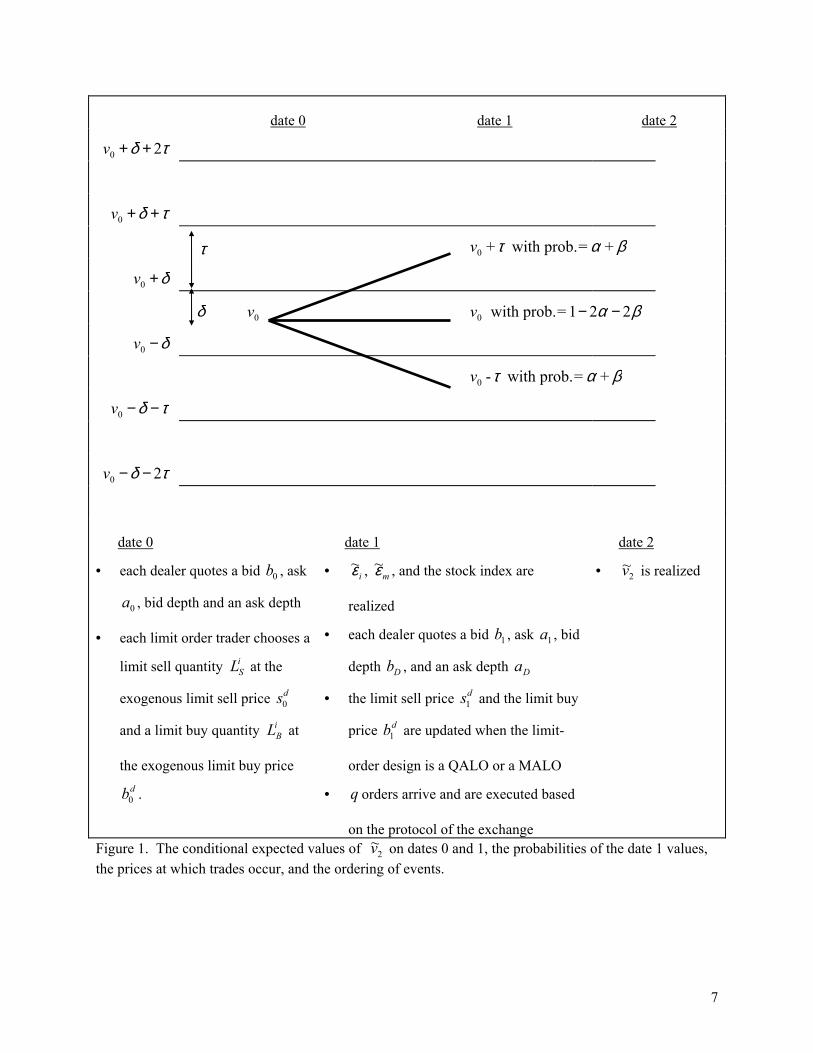
where τ is the tick size, meaning that trades occur at prices which are τ dollars apart (see Figure 1). The

nearest trading prices are half of a tick δ τ≡ 2je above and below the conditional means.

Three classes of economic agents exist: identical competitive dealers, strategic limit-

order traders (LO traders), and exogenous market-order traders (MO traders). The sequence of events in

the model is as follows: On date 0, each competitive dealer quotes a bid price b , ask price , bid depth,

and ask depth. Then, the i LO trader conjectures the quantities submitted by other LO traders, and

chooses a limit sell quantity at an exogenous limit sell price and chooses a limit buy quantity

N M N L

0 a0

th

LSid sd

0

LBid at an exogenous limit buy price b . Here the superscript denotes the design of the limit order

(RLO, MALO, or QALO). On date 1, the systematic innovation

d0 d

~εm , the idiosyncratic innovation ~εi , and

6

date 0 date 1 date 2

v0 2+ +δ τ

v0 + +δ τ

τ v + with prob.= +0 τ α β

v +0 δ

δ v 0 0 v 1 2 2 with prob.= − −α β

v −0 δ

v - with prob.= +0 τ α β

v − −0 δ τ

v 2− −0 δ τ

date 0 date 1 date 2

• each dealer quotes a bid b , ask

, bid depth and an ask depth

0

a0

• each limit order trader chooses a

limit sell quantity at the

exogenous limit sell price

and a limit buy quantity at

the exogenous limit buy price

.

LSi

sd0

BiL

bd0

• ~εi , , and the stock index are

realized

• each dealer quotes a bid b , ask a , bid

depth b , and an ask depth a

1 1

• the limit sell price and the limit buy

price b are updated when the limit-

order design is a QALO or a MALO

sd1

d1

• orders arrive and are executed based

on the protocol of the exchange

q

• ~v2 is realized

Figure 1. The conditional expected values of ~v2 on dates 0 and 1, the probabilities of the date 1 values, the prices at which trades occur, and the ordering of events.

~εm

D D

7

a stock index innovation are realized. We assume that the systematic innovation in the individual security

value ~εm

1

can be calculated from a broad stock index innovation.12 Then each dealer quotes a new bid

price b , ask price a , a bid depth b , and an ask depth . Finally, a quantity 1 D aD~q of market orders

arrives and all orders are executed according to the protocol of the security exchange.13 On date 2, the

terminal value ~v2 is realized.

Limit orders are submitted at time 0 and are either executed at time 1 or not at all. It is assumed

that LO traders do not monitor their limit orders on date 1 and hence cannot cancel or alter the terms of

their limit orders. Limit prices of the MALOs and QALOs are automatically updated on date 1 without

any intervention by the LO traders, while those of the RLO remain fixed.

We assume that ~q is uniformly distributed on [-Q, Q], is independent of ~v1 , and is able to

exhaust the total depth supplied by limit-orders and dealers Q a L Q b LD Si

iD B

i

i

> + − < +FH

IKJ∑ ∑ and

a0 0 h

G .

The last part of the assumption simply restricts attention to the interesting case, which is when it is

possible to exhaust the total depth.14 For simplicity, we do not model the arrival of market orders on date

0 before limit prices have had an opportunity to become mispriced. We impose the convention that limit

orders to sell are originally submitted at the ask price c and limit orders to buy are originally

submitted at the bid price c .

sd =

b bd0 0= h

Because dealers are competitive, the date 0 and date 1 inside quotes are δ above and δ below

the conditional mean on each respective date, i.e.,

12 The idea we have in mind for how to calculate ~εm is to estimate a “market model regression” of the innovations in an individual security value on the innovations in a broad stock index. The estimated regression equation, with an estimated alpha and beta, provide a simple means to translate stock index innovations into an estimate of the systematic innovation in the individual security value ~εm . 13Positive values of ~q denote market buy orders and negative values of ~q denote market sell orders. 14 The dealer depth is decreasing in their risk aversion and the limit-order trader quantity is decreasing in their risk aversion. Hence, this assumption can be reformulated in terms of exogenous parameters as a joint restriction on the

8

a v a vb v b v

0 0 1 1

0 0 1 1

= + = += − = −

δ δδ δ

, ,, .

Note, the date 0 quote midpoint is b g and the date 1 quote midpoint is .

Hence, the innovation in quote midpoint between dates 0 and 1 is equal to the total innovation in the

security value

b a v0 0 2+ =/ 0 1b a v1 1 2+ =b g /

ε ε ε≡ + =m i v1 − v0 . The total innovation will serve as the basis for updating QALO limit

prices.

1.2 The Trade Protocol

The trade protocol specifies how trades are matched and at what prices execution occurs. See Table 1 for

a list of rules defining the protocol for our model.

1. Pricing on ticks. All trades of the riskless and risky assets are executed at prices equal to ticks, which are integer multiples of τ. 2. Price priority. Market buys (sells) are crossed at the lowest (highest) tick offered by limit sells (buys) or dealers selling (buying). 3. Fair market. If limit orders and dealers are willing to trade at the same price tick, then limit orders get first priority. Limit orders are executed only at limit prices. Dealers may trade against limit orders, so long as all market orders are executed. 4. Pro-rata Rationing. At any tick, if the aggregate size of limit buys (sells) exceeds either market sell (buy) or dealers’ willingness to sell (buy), then each limit buy (sell) receives a pro-rata share. Similarly, if the aggregate demand of dealers exceeds the market orders net of limit orders, the percentage of an individual dealer's demand which is filled is equal to the ratio of the net market orders to aggregate dealer demand. 5. Uniform Dealer Price. All dealer trades with market orders are at a single tick, which may be different from limit prices.

Table 1. The Trade Protocol Rule 1 is self explanatory given the structure of the model shown in Figure 1. Rule 2 says that market

orders trade either at the limit price or at the dealer quote, depending on which offers the best price. The

first part of Rule 3 says that limit orders have priority over the dealer when they are both willing to trade

at the same price tick. The second part rules out the possibility that a limit order may trade at a price

risk aversions of the dealers and limit order traders such that they jointly choose a total depth which is less than Q (in absolute value).

9

which is more advantageous (to the limit-order trader) than the limit price.15 The final part of Rule 3

allows dealers to pick off any mispriced limit orders, so long all market orders are executed.

Rule 4 recognizes that excess demand or supply may exist because of prices set on ticks (Rule 1).

In practice, orders with identical limit prices are ordered on the basis of time of arrival and market orders

are executed against those limit orders first to arrive. In this model, limit orders arrive simultaneously at

time 0 and pro-rata rationing is a simple substitute for time priority.

Rule 5 has the dealer set a single “clean-up” price to execute remaining market order not executed

against limit orders. Together, the trade protocol of Rules 1-5 defines the formal exchange setting of this

model.

1.3 The Dealers’ Problem

Dealers in this model are competitive and choose the quantities to trade on date 1 conditional on

knowledge of ~q and ~v . Dealers are assumed to be risk averse with a mean-variance indirect utility

function.16 Given a fixed price p, a dealer’s time 1 objective function in a classical Walrasian setting

without discrete price ticks is

1

Maximize E[ Var[2θ

~ | , ] ~ | , ]W v q B W v q1 22− ,1 (1)

where date 2 wealth is ~ (~ )v pi2 1 2= − −θW W , >0 represents dealer selling, is date 1 wealth, and θ i W1 B

is the dealers risk aversion parameter. Differentiating with respect to , aggregating over all of the

dealers, and solving for price we obtain the aggregate Walrasian supply schedule of dealers

θ i

p v b b BNw

D

( )θ θ= + ≡ σFHGIKJ1 1

2 where , (2)

and θ is aggregate dealer trade. The price is a continuous and increasing function of θ.

15 This happens occasionally on the NYSE in the case of a large block trades. 16 The standard utility-based justification of mean-variance analysis is quadratic utility. Unfortunately quadratic utility exhibits increasing absolute risk aversion. Epstein (1985) drops the independence axiom of expected utility theory and then demonstrates that only extremely weak assumptions of differentiability, continuity, and boundedness are required in order for a direct utility function with decreasing absolute risk aversion to rigorously justify mean-variance analysis.

10

With pricing on ticks, the aggregate Walrasian supply schedule must be modified. The procedure

for doing this is illustrated in Figure 2. The dashed line is the aggregate Walrasian supply schedule

pw ( )θ plotted against aggregate dealer trading θ on the x-axis. The set of price ticks, ... $30.15, $30.16,

$30.17, $30.18, ..., are plotted on the y-axis and are $0.01 apart in this example. The aggregate dealer

supply schedule on discrete ticks is the set of solid line segments, with one line segment on each price

tick. This schedule is obtained by rounding up from the Walrasian schedule to the nearest tick for θ > 0

and similarly rounding down for θ < 0 .

Formally, the aggregate dealer supply schedule on discrete ticks p v( , )θ 1 is obtained by

introducing a tick function T( )θ as follows

p v v T Tn n b

n n b( , ) ( ) ( )θ θ θ

τ δ τ δ θ θτ δ τ δ θ θ1 1

n

n

where Min s. t. when >

Max s. t. when = + ≡

+ + ≥

− − ≤ <

RS|T|

∈ ℵ

∈ ℵ

l ql q

0

0 (3)

and ℵ is the set of integers. The constraints in (3) ensure that dealers’ willingness to trade at the price

is greater than or equal to the quantity traded θ. When their willingness to trade exceeds p v1θ,b g θ (in

absolute value), then Rule 4 of the exchange protocol applies and each dealer receives a pro-rata share of

the aggregate trade θ.

Ask and bid depths are the largest aggregate quantities that dealers are will to trade at ask and bid

prices, respectively. From Figure 2, it is clear that the ask depth is the point where the Walrasian schedule

intersects the level of the date 1 ask price v1 +δ and the bid depth is analogous. In Figure 2, the

aggregate dealer supply schedule on discrete ticks can be written as

. p v

v b qv b qv b qv qv a qv a q

D D

D D

D

D

D D

D D

θ

δδδδδδ

, 1

1

1

1

1

1

1

5 53 3

00

3 35 3

b g =

− <− <− <+ <+ <+ <

R

S

|||||

T

|||||

when when

when when

when when

bb

aaa

3

5

≤≤≤≤≤≤

11

Formally, the bid and ask depths are obtained by setting n in the constraints in (3) and

solving these as equalities for θ. Hence, the endogenous dealers’ ask depth and bid depth b are

= 0

aD D

aB

N

bB

N

D

D D

= FHGIKJ

= −FHGIKJ

δ

σ

δ

σ12

12

.D

These expressions for dealer depths can be interpreted as a risk premium per unit risk c times the

aggregate risk tolerance .

δ σ/ 12 h

N BD /b g

1.4 Alternative Limit-Order Designs

Having laid the foundation, we can formally define the three alternative types of limit orders.

Definition: Regular Limit Order (RLO). A limit order with a constant limit price. Specifically:

b b s sR R R1 0 1 0= = .R

+

+

d

Definition: Quote Adjusted Limit Order (QALO). A limit order with a limit price adjusted for the

innovation in quote midpoint. Specifically:

b b s sQ Q Q Q1 0 1 0= =+ ε ε.

Definition: Market Adjusted Limit Order (MALO). A limit order with a limit price adjusted for the

systematic innovation. Specifically:

b b s sM MM

M MM1 0 1 0= =+ ε ε .

These three designs differ in how they update (or fail to update) the limit buy and sell prices and

thus affect the chances that the two limit prices will bracket the updated public valuation . For a limit

order of design , we say the “fairpriced” state has been realized when the two limit prices bracket the

updated public valuation . We say the “underpriced” state is realized when both limit

prices are less than the updated public valuation c . And we say the “overpriced” state is

realized when both limit prices are greater than the updated public valuation c . These latter

two states, taken as a single event, comprise what we call the “mispriced” state.

v1

v h

d

s v bd1 1 1> >c h

b s vd d1 1 1< < h

s bd d1 1 1> >

12

The performance of the three designs in achieving the fairpriced state vs. the mispriced state is

summarized in Table 2 below for each of the five joint realizations of ~ ,~ε εm ib g . Table 2

Performance of Three Limit Order Designs by the Five Joint Realizations of ~ ,~ε εm ib g . Realization: Probability RLO MALO QALO

Underpriced Fairpriced Fairpriced Underpriced Underpriced Fairpriced

Fairpriced Fairpriced Fairpriced Overpriced Overpriced Fairpriced

Overpriced Fairpriced Fairpriced

Probability of Mispriced (Underpriced or Overpriced):

ε ε ετ τ ατ τ β

α βτ τ βτ τ α

α β

= +

= += += + − −

− = + −− = − +

= +

~ ~

( )( )

m i

R M

00

0 0 0 1 2 20

0

2 2Γ Γ = =2 0β Γ Q

Because RLO limit prices are never revised, RLOs are underpriced when ε τ= and overpriced when

ε τ= − . Hence, the probability of mispricing under RLOs is Γ . MALO limit prices are

correctly revised whenever the idiosyncratic innovation is zero (i.e.

R = +2α 2β

ε ε= m ). MALOs are underpriced

when ε m = 0 & ε τ= and overpriced when ε m = 0 & ε τ= − . Hence, the probability of mispricing

under MALOs is .17 Of course, QALO limit prices are always revised correctly. Hence, the

probability of mispricing under QALOs is

Γ M = 2β

Γ Q = 0 .

Although the limit order design affects the probability of either underpricing, overpricing, or

fairpricing, once one of the three states has been realized, the design d has no additional significance.

For example, a RLO, MALO, and QALO in the underpriced state each has the same chance of full or

partial execution and the same probability distribution for profits.

d

2 Fixed Limit-order Quantities

2.1 The Direct Effect on Ex-Ante Profits for All Three Classes of Agents

17 If the security and the market index were perfectly correlated, then MALOs and QALOs would be identical. Of course the interesting case in when the security and the market index are not perfectly correlated.

13

In this section, we analyze the ex-ante profits of each of the three classes of agents under three limit-order

designs in partial equilibrium, holding the limit-order quantities fixed. In the next section, we expand the

analysis to a full equilibrium in which the limit-order quantities are endogenously determined.

In our model, each state of the world results in either one or two transactions. It turns out that a

limit buy and a limit sell never execute in the same event. This permits us to partition events into (1) the

limit buy side, (2) the limit sell side, or (3) the no limit order side. Similarly, it turns out that market buys

and market sells never execute together18 and dealers never buy and sell in the same event. Hence, events

can alternatively be partitioned into (1) the market buy side, (2) the market sell side, or (3) the no market

order side. Likewise events can also be partitioned into (1) the dealer buy side, (2) the dealer sell side, or

(3) the no dealer side. Interestingly these nine sides of the exchange cannot be packaged up into two (or

three) overall sides of the exchange. For example, in some events both market buys and limit sells

execute, whereas in other events both market buys and limit buys execute.

We obtain considerable simplification from the symmetry of the distributions and symmetry of

the trade protocol (asymmetry of a LO trader’s strategy is permitted in this section). Every event on the

limit sell side has a mirror image event on the limit buy side. Similarly, every event on the market buy

side has a mirror image on the market sell side and every event on the dealer buy side has a mirror image

on the dealer sell side. Hence for simplicity, we concentrate our exposition on the limit sell side, the

market buy side, and the dealer sell side. The limit buy side, the market sell side, and the dealer buy side

are incorporated by analogy. We wish to emphasize that we are not adding any restrictions on any of the

agents in the model.

Let be the aggregate quantity of limit sells and let L LS Si

i

≡∑ L LB Bi

i

≡∑ be the aggregate

quantity of limit buys. Let E L Lcd

S Bπ ,b g be the aggregate expected profits for traders of class

c

18 Chakravarty and Holden (1995) permit market buy orders to cross with market sell orders. Our results are not sensitive to this issue since you can always think of q as the net quantity of market orders after market buy orders and market sell orders have already been crossed.

14

(dealer, LO traders, MO traders) where limit sells and limit buys of design have been

submitted. This profit function can be decomposed as follows

LS LB d

E L L E L L E L Lcd

S Bd

c S Bd

S BCπ π π, , | , ,b g c h b g b= − +1 Γ Γfair |mg is

− Γ

(4)

where Γ d is the probability of mispricing under design and “fair” and “mis” mean conditional on

being in the fairpriced and mispriced states, respectively. Note that the design determines the

probability of the mispriced state

d

d

Γ d (and the probability of the fairpriced state 1 d ), but that the

expected profits for each class in each of these states E cπ πd i are

independent of the design d . The three alternative designs have a strict ordering in terms of the

probability of mispricing

E L L L Lc S B S B, | , |b g b gmis and fair

+ 2βΓ Γ ΓQ M R= = =0 2 2 < < β α . (5)

Again, QALOs are never mispriced, MALOs are mispriced due to idiosyncratic innovations and RLOs

are mispriced due to both idiosyncratic and systematic innovations.

Straight forward calculations show that the difference in expected profits between the fairpriced

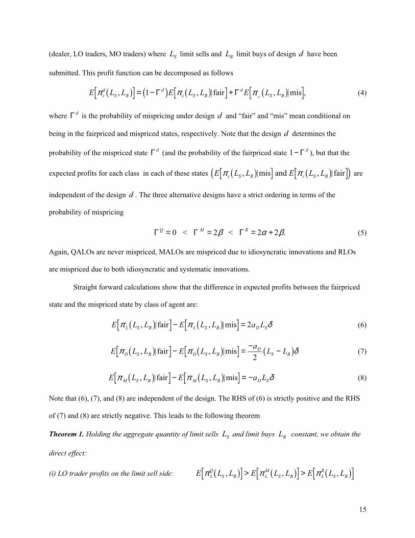
state and the mispriced state by class of agent are:

E L L E L L a LL S B L S B D Sπ π, | , |b g b gfair mis− = 2 δ (6)

E L L E L L a L LD S B D S BD

S Bπ π, | , |b g b g bfair mis− = − −2

δg (7)

E L L E L L a LM S B M S B D Sπ π, | , |b g b gfair mis− δ= − (8)

Note that (6), (7), and (8) are independent of the design. The RHS of (6) is strictly positive and the RHS

of (7) and (8) are strictly negative. This leads to the following theorem

Theorem 1. Holding the aggregate quantity of limit sells and limit buys constant, we obtain the

direct effect:

LS LB

(i) LO trader profits on the limit sell side: E L L E L L E L LLQ

S B LM

S B LR

S Bπ π π, ,b g b g b g> > ,

15

(ii) Dealer profits on the dealer sell side: E L L E L L E L LDQ

S B DM

S B DR

S Bπ π π, ,b g b g b g< < ,

(iii) MO trader profits on the market buy side: E L L E L L E L LMQ

S B MM

S B MR

S Bπ π π, , ,b g b g b g< <

and analogous results hold for LO trader profits on the limit buy side, Dealer profits on the dealer buy

side, and MO trader profits on the market sell side.

Theorem 1 shows that the direct effect is a gain for LO traders at the expense of dealers and MO

traders. Further, the relative ranking of the three designs is driven by the probability of mispricing.

2.2 Profit Margins and the Quantity Executed

Define the profit margin of a limit order as the gain per unit executed. For limit buys and limit sells of

design , these are dp v b

p v sBd d

Sd d

= −

= − −

1 1

1 1c h,

respectively. For example, consider a RLO to sell, for which the limit sell price is held constant

. Further, suppose the realized date 1 value is v vs s vR R1 0 0= = +δ 1 0= −τ . Then the limit sell obtains a

“windfall” profit margin

. p v s v vSR

d= − − = − − − + =11

0 0 3c h b gc hτ δ δ

More generally, for limit buys and limit sells of design , the pair of profit margins c obtained

by the LO trader falls into one of three cases

d p pBd

Sd, h

p pv ss bb v

Bd

Sd

d

d d

d

,,

,, .

c hb gb gb g

=− >

− >

RS|T|

3

3

1 1

1 1

1 1

δ δδ δδ δ

when when > v >

when 1

In the underpriced state, a limit buy (sell) makes a windfall gain of 3δ (negative profit of −δ ). In the

overpriced state, the opposite result is obtained. In the fairpriced state, both a limit buy and a limit sell

make a gain of δ .

16

There is a very interesting interaction between profit margins and the quantity executed. As a

numerical example, suppose the ask depth a = 3 shares, the bid depth = -3 shares, the upper bound

on market buy orders = 12 shares, and the total quantity of limit sells submitted = 7 shares. Figure

3 illustrates the execution of these limit sells at a negative profit margin, a normal profit margin, and a

windfall gain margin. The total quantity of limit sell orders executed (the y-axis) is plotted as a function

of the quantity of market buy orders that arrive (the x-axis).

D bD

Q LS

q

First consider the normal profit margin (from the fairpriced state) shown by the long-

dashed line. As the market buy quantity increases from 0 shares to 7 shares, the limit sell quantity

executed rises in tandem at a 45 degree angle. When exceeds 7 shares, the limit sell quantity executed

remains constant at 7 shares representing 100% execution of the limit sells submitted.

pSd = δ

q

q

Next consider the windfall profit margin (from the overpriced state) shown by the

short-dashed line. For q in the interval from 0 shares to the ask depth = 3 shares, the dealer trades all

of the market buys at the ask price

pSd = 3δ

aD

a v1 1= +δ and undercuts the limit sell price . As

increases from 3 shares to 10 shares, the limit sells get the excess above the ask depth and the quantity

executed rises at a 45 degree angle. For greater than 10 shares, 100% of the limit sells execute at the

limit sell price and the dealer sets a clean-up price at which the dealer

trades the rest of the market buys. Comparing the two profit margins, the limit sell quantity executed with

a normal profit margin is always greater than or equal to the quantity executed with a windfall profit

margin.

s vd1 1 3= + δ

v1, g

q

q

s vd1 1 3δ= + p q sharesb − 7

Finally consider the negative profit margin (from the underpriced state) shown by the

solid line. When q = -3 shares, the dealer buys all of these market sells at the bid price b v

pSd = −δ

1 1= −δ . This

exhausts the quantity that the dealer is willing to buy at v1 −δ and the dealer does not buy any of the

limit sells even though a profit of δ per share could be obtained by doing so. As q increases from -3

17

shares to 0 shares, the dealer buys all of these market sells and picks off limit sells at the limit sell

price . As q increases from 0 shares to 4 shares, the dealer picks off 3 limit sells and the q

market buys execute against limit sells. Thus, quantity of limit sells executed rises at a 45 degree angle as

increases from -3 shares to 4 shares. Finally, for q above 4 shares, 100% of the limit sells execute.

3−q

LB

L LS Bδ

g

s vd1 1= −δ

q L LS Sd

S, , ,

q

:

,

q X

q b

q a

for all

for

for b

q

(

ii

i

L

b

a

,L L

X

X S

>

>g

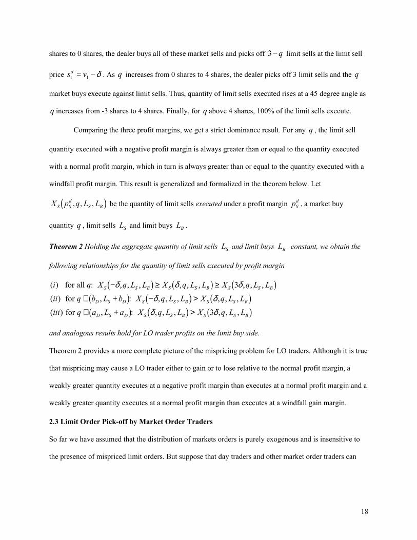
Comparing the three profit margins, we get a strict dominance result. For any , the limit sell

quantity executed with a negative profit margin is always greater than or equal to the quantity executed

with a normal profit margin, which in turn is always greater than or equal to the quantity executed with a

windfall profit margin. This result is generalized and formalized in the theorem below. Let

be the quantity of limit sells executed under a profit margin , a market buy

quantity , limit sells and limit buys .

q

X p Bc h pSd

S LB

Theorem 2 Holding the aggregate quantity of limit sells and limit buys constant, we obtain the

following relationships for the quantity of limit sells executed by profit margin

LS

) , , , , , , , ,

( ) : , , , , , ,

( ) , : , , , , , ,

i q L L X q X q

L X q L L q L L

ii L X q L L q L L

S S B S S B S

D S D S S B S S B

D S D S S B S B

− ≥ ≥

∈ + −

∈ +

δ δδ δ

δ δ

b g b g bg b g b g

b g b b

3

3

g

and analogous results hold for LO trader profits on the limit buy side.

Theorem 2 provides a more complete picture of the mispricing problem for LO traders. Although it is true

that mispricing may cause a LO trader either to gain or to lose relative to the normal profit margin, a

weakly greater quantity executes at a negative profit margin than executes at a normal profit margin and a

weakly greater quantity executes at a normal profit margin than executes at a windfall gain margin.

2.3 Limit Order Pick-off by Market Order Traders

So far we have assumed that the distribution of markets orders is purely exogenous and is insensitive to

the presence of mispriced limit orders. But suppose that day traders and other market order traders can

18

quickly take advantage of stale limit orders. Intuitively, this would exacerbate the mispricing problem for

limit order traders.

To investigate further, let’s assume that market order submitters are good at observing19 and

exploiting mispriced limit orders. For this subsection only, assume that when limit sells are underpriced,

then market order submitters who were otherwise included to submit a market buy order in the range

[ ]0, SL , increase their market buy order up to the maximum size , in order to optimally profit off of

the stale limit sell (and may the analogous change on the market sell – limit buy side of the market). The

following theorem compares the profits of all three parties when these “semi-endogenous” market order

submitters exploit mispriced limit orders compared the base case of purely exogenous market order

submitters who don’t.

SL

Theorem 3 Holding the aggregate quantity of limit sells and limit buys constant, when market

order submitters exploit mispriced limit orders the following happens

LS LB

(i) market order submitters reduce their loss by 2 2 2

ds sL LQ

δ Γ

compared to the base case,

(ii) limit order submitters decrease their profit by 2 2 2

ds sL LQ

δ Γ

compared to the base case,

(iii) dealers have zero change in profit compared to the base case,

and analogous results hold for the market sell – limit buy side of the market.

This theorem confirms the intuition that the magnitude of the mispricing problem is increased

when market order submitters observe and exploit mispriced limit orders. Notice that the magnitude of the

change in profits is proportional to the probability that limit sells are underpriced under design d 2dΓ .

Thus, QALOs and MALOs have a bigger direct effect when market orders exploit mispriced limit orders

compared to the base case. It turns out that QALOs and MALOs also have a bigger indirect effect, as we

19

shall see in the next section. We shall return to discussing the impact of market orders exploiting

mispriced limit orders at that time.

3 Endogenous Limit-Order Submission

3.1 An Analytic Solution

Section 2 is a partial equilibrium analysis because the quantity of limit orders is held constant. In this

section, the quantity of limit orders submitted is endogenous and we analyze the resulting equilibrium

under each design.

As noted before, the joint distribution of b is symmetric and the trade protocol treat buys

and sells in a symmetric manner. This motivates the view that individual LO traders may be interested in

following a symmetric strategy, defined as submitting the same (absolute) size limit buy and limit sell

ε εm i, g

L LSid

Bid=e j . In order to obtain an analytic solution, we focus on symmetric equilibria, defined as an

equilibrium in which every individual LO trader follows a symmetric strategy L L iSid

Bid= for all je .20

To simplify the notation, let L L LidSid

Bid≡ =

Lod th

th

be the size of the symmetric strategy chosen by the i LO

trader under design . Let be the i LO trader’s conjecture about the aggregate size of the

symmetric strategy followed by all of the other LO traders. LO traders are assumed to have a mean-

variance indirect utility function.21 The i LO trader’s problem is

th

d

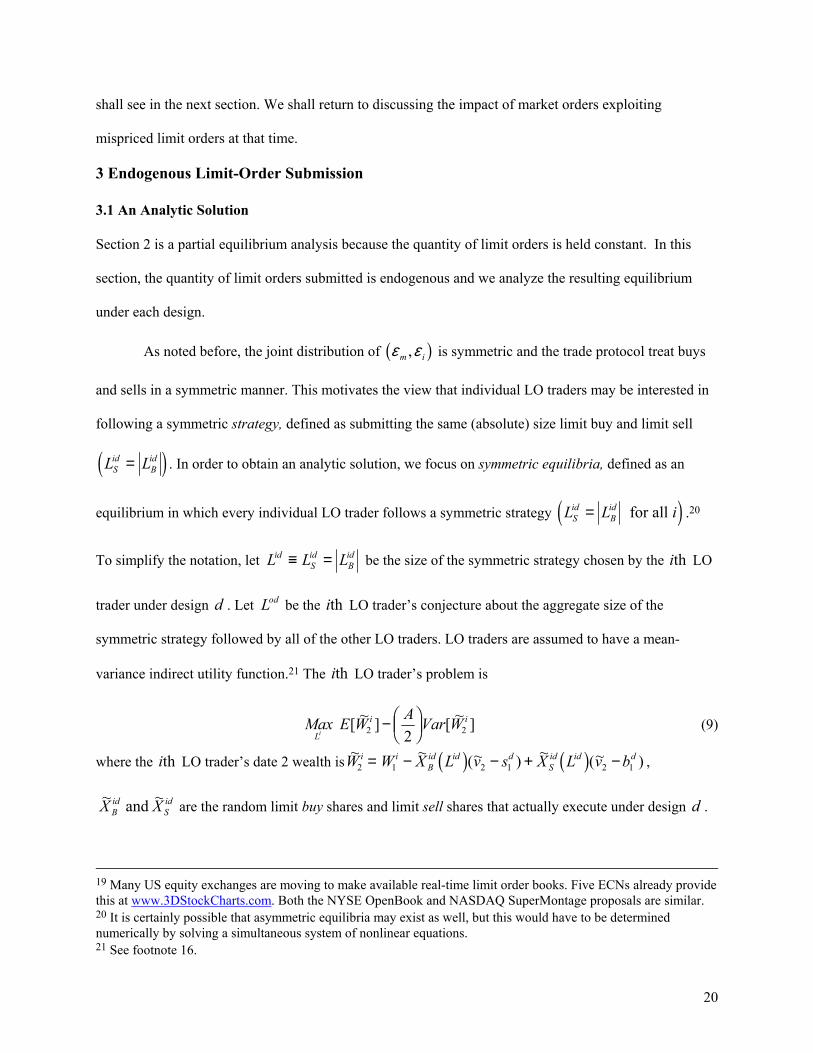
Max E W A Var WL

ii

[ ~ ] ~ ]2 22− i[FHGIKJ (9)

where the LO trader’s date 2 wealth isith ~ ~ (~ ) ~ (~ )X L v s X L v bi iBid id d

Sid id d

2 1 1 1= − − + −c h c h2 2W W ,

~ ~X Bid and X S

id are the random limit buy shares and limit sell shares that actually execute under design . d

19 Many US equity exchanges are moving to make available real-time limi der books. Five ECNs already provide t or

this at www.3DStockCharts.com. Both the NYSE OpenBook and NASDAQ SuperMontage proposals are similar. 20 It is certainly possible that asymmetric equilibria may exist as well, but this would have to be determined numerically by solving a simultaneous system of nonlinear equations. 21 See footnote 16.

20

We calculate the expected terminal wealth and variance of terminal wealth. Since both the

quantity executed and the probability of each state are functions of Lid , we obtain a quadratic expression

for expected wealth and a quartic expression for the variance of wealth. Substitu

ting into the objective

function, taking the derivative with respect to

set , we obtain a cubic equation for the first order condition

id id id+ =3 2c h c h (10)

is leads to the following theorem.

is defined in the

Lid

L N LodL

id= −1b g

Theorem 4 Wh

appendix), there is an unique symmetric

in

Theorem 4 pro

LO trader to be unique. It is interesting th

Γ d DQ N>G Jσ 1

fec

letely

, and using the fact that all LO traders are identical to

FOC L c L c L L c( ) ,≡ + +3 2 1 0 0

where the coefficients c c c c3 2 1 0, , , and are given in the appendix. Th

cidc h

en LO traders have a risk aversion coefficient A A> * (where A*

equilibrium with a solution:

Q a Q ND d D−L OR12σ

L N B

whenB

id L= N Q>

ST|

2

02

Γ

δ

δ.

ides a sufficient condition for the optimal quantity of limit orders chosen by the v

d

BFH

IKδ

2

2

Unique root of FOC when

Q Nd D

M P ≤|||

, 0

12

Γ

σ

,

at when the probability of mispricing under design is very

large , then LO traders find it optimal to avoid submitting a limit order and the market

quidity fails comp . As long as the probability of mispricing falls below this

t

for limit order supplied li

boundary, then there is an interior optimum.

3.2 The Indirect Ef

Next we use the analytic solution to analyze the indirect effect of alternative designs. This leads to the

following theorem.

21

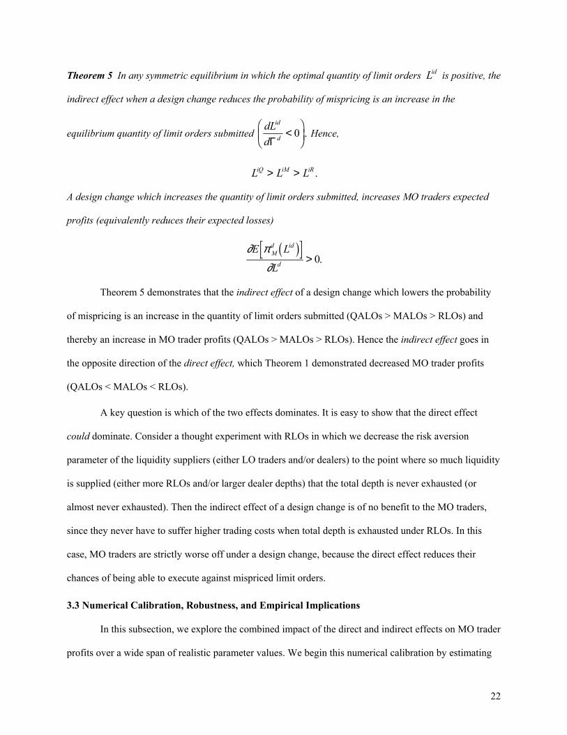
Theorem 5 In any symmetric equilibrium in which the optimal quantity of limit orders Lid is positive, the

equilibrium quantity of limit orders submitted

indirect effect when a design change reduces the probability of mispricing is an increase in the

dLidFd dΓH K

L L LiQ iM iR> > .

<G IJ0 . Hence,

A design change which increases the quantity of limit orders submitted, increases MO traders expected

profits (equivalently reduces their expected losses)

∂L

d id

d

c h> 0.

Theorem 5 demonstrate

∂ πE LM

s that the indirect effect of a design change which lowers the probability

f misp

s in

A key question is which of the two effects dominates. It is easy to show that the direct effect

parameter of the liquidity suppliers (either LO traders and/or dealers) to the point where so much liquidity

is supplied (either more RLOs and/or larger dealer depths) that the total depth is never exhausted (or

almost never exhausted). Then the indirect effect of a design change is of no benefit to the MO traders,

3.3 Numerical Calibration, Robustness, and Empirical Implications

In this subsection, we explore the combined impact of the direct and indirect effects on MO trader

profits over a wide span of realistic parameter values. We begin this numerical calibration by estimating

o ricing is an increase in the quantity of limit orders submitted (QALOs > MALOs > RLOs) and

thereby an increase in MO trader profits (QALOs > MALOs > RLOs). Hence the indirect effect goe

the opposite direction of the direct effect, which Theorem 1 demonstrated decreased MO trader profits

(QALOs < MALOs < RLOs).

could dominate. Consider a thought experiment with RLOs in which we decrease the risk aversion

since they never have to suffer higher trading costs when total depth is exhausted under RLOs. In this

case, MO traders are strictly worse off under a design change, because the direct effect reduces their

chances of being able to execute against mispriced limit orders.

22

the price volatility, market order size, and number of dealers parameters for a high volume stock

(Microsoft [MSFT]) and a low volume stock (BEI Medical System Company, Inc. [BMED]). W us

that day, Microsoft had 51,124 trades with ance of the trade-to-t rice change 1

e e all

of the trades for both stocks on September 4, 2001 from the NYSE Trade and Quote (TAQ) database. On

2a vari rade p MSFTσ = 0.0019.

By contrast, BEI Medical Systems had 30 trades with a variance of trade-to-trade price change 1BMEDσ =

0.0013. We used the 90th percentile of trade size to estimate the market order size upper bound Q ,

because this is a frequently-encountered large trade size and is less likely to be an outlier than taking

very large

2

the

st trade of the day. This yielded MSFTQ = 1,000 shares and BMEDQ = 2, res. Surprising

BMED had larger trade sizes at nearly all percenti s (20%, 30%, …, 90%) despite having radically

smaller volume. Perhaps, this is due to Microsoft receiving a much large proportion of small orders from

Report at www.nasdaqtrader.com

050 sha ly,

individual day traders. To estimate the num Share Volum

le cutoff

dealers, we examber of ined the Monthly e

for the month of September 2001. MSFT had ,D MSFTN = 29 broker-

dealers with 1% or more volume and BMED had ,D BMEDN = 11 broker-dealers with 1% or more volume.

We set the ti ck size = $.01. We set the ersion τ LO trader risk av 1=A and dealer risk aversion 1B =

low are

, ,nd L BMEDN N0.1 0.1, 11.L MSFTα , 29, aβ= = =

=

ma

ke both market order traders and limit order traders better

,

both of

em as

which consistent with historical estimates of the market risk premium and other macroeconomic

data.22 The remaining parameters are not readily observable, but it turns out the main results be

qualitatively similar over a wide range of values for the remaining parameters. Somewhat arbitrarily, we

set th

For both MSFT and BMED parameters, our key finding is that the indirect effect dominates the

direct effect and yields higher profits for market order traders (QALO > MALO > RLO). This

demonstrates that adjustable limit orders can

off .

22 See the numerical simulations for representative agents in Sundaresan (1989) and Leland (1992).

23

Next, we p siserform sensitivity analy on these results and find them to be very robust over a wide

g eters, the indirect effect dominates the direct

effect over the following parameter ranges:

• MO size upper bound 100 shares (one round lot) to 10,000,000 shares (1,000 blocks),

• innovation probabilities and from .0001 to 0.5,α

ran e of parameters. For both MSFT and BMED param

Q from

β

• and fromA B

τ from $.001 to

risk aversions 1 to 50,

• tick size 18 , $

• number of dealers DN and number of LO traders LN from 1 to 250, and

• price volatility 21 from .0002 to 1σ .

The reverse result, when the direct effect dominates the indirect effect, is obtained for only the most

extreme parameter values: when Q < 80 shares for MSFT, when 40Q < shares for BMED, when

21 .0σ < 1 D D

for BMED, etc. Thus, we conclude that over a wide span of realistic parameter values the indirect effect

dominates the direct effect, yielding higher profits for market order traders (QALO > MALO > RLO). In

summary, adjustable limit orders are predicted to yield higher profits (or smaller losses) for both market

order traders and limit order traders.

In section 2.3, we analyzed what would happen if market order submitters are good at observing

and exploiting mispriced limit orders. We wish to determine the combined impact of the direct and

indirect effects in this scenario. For both MSFT and BMED parameters, we find that MO trader profits

are changed by less than 1%. Thus, the key findings and sensitivity analysis are essentially unchanged

from above.

Our model abstracts away from asymmetric information, inventory effects, and other frictions.

While incorporating these features into the model would make it needlessly complex, we would like to

discuss how the results would be impacted if the model were extended in these directions. Adding

001 for MSFT, when 2 .00002σ < for BMED, when 300N > for MSFT, when 500N >

24

asymmetric information would have two effects. First, the slope of the aggregate Walrasian supply

schedule of dealers in equation (2) would be steeper to allow dealers to recover losses to privately

informed traders. This would reduce the depth Da supplied by dealers. In Theorem 1, the profit

differentials would be smaller, but the directions of the inequalities would be the same. In Theorem 2

size of the intervals with strict inequalities in (ii) and (iii) would smaller, but the results would

qualitatively be the same. Theorem 3 would be unchanged. The second general effect is that the limit

order quantity endogenously determined by LO traders in Theorem 4 would be smaller due to losses to

privately informed traders. Adding inventory effects, order proce ng costs, or other dealer costs, wo

also increase the slope of the aggregate supply schedule (reducing the depth

, the

ussi ld

Da ) and/or increase the

sprea etd b ween the de quotes. To gauge the impact of these changes on the numerical calibration, an insi

O

at

cel

e

e

n

asb

increase in the slope of the supply schedule is similar to what would happen when dealer risk aversion B

is increased. Also a reduction in limit order quantity by LO traders is similar to what would happen if L

trader risk aversion A increased or if the number of LO traders LN increased. From the sensitivity

analysis above, we see that the indirect effect dominates the direct effect over wide variations in B , A ,

and LN .

The model makes a number of predictions that could be empirically tested about the impact th

would result from the introduction of adjustable limit orders. First, it predicts that the quantity of limit

order submissions should increase. A subtle point is that adjustable limit orders may substitute for ca

and resubmit activity, so cancels and resubmits should be removed. The NYSE System Order Data

(SOD) provides all of the data needed to make this adjustment. Second, the numerical calibration exercis

predicts that market order profits should increase (i.e., smaller losses). Thus, effective spreads should

decrease for market orders. The new SEC rule (11Ac1-5) which mandates disclosure of order-execution

performance provides all of the data needed to test this implication

. Specifically, all market centers

alist firms, and ECNs) are required to post on their web site monthly data on the

effective spread of every stock that they trade. Further, this must be broken down by: (A) market orders

(exchanges, speci

25

vs. limit orders, (B) limit order price categories (executable, inside-the-quote, at-the-quote, behind-the

quote), and (C) by order size categories. Finally, the model predicts that the total volume of trade should

increase. This could be tested with standard trade and quote data.

. Con

oduction of

able limit orders a

ality f

e

djustable limit orders may be view as an effort to improve the efficiency of

the trading process by automating part of it. The computerized updating of adjustable limit orders is a

substitute for human time and attention by LO traders devoted to monitoring and updating RLOs. This

suggests that we should scrutinize the entire trading process to see if there are other opportunities to

automate part of the process.

4 clusion

We analyze three alternative designs of limit orders. Not only do LO traders gain from having “more

efficient” limit orders, but it is possible and likely for MO traders to gain overall from the intr

adjustable limit orders.23

The ability to program a computer to track market conditions, cancel an old limit order, and

immediately resubmit a new limit order at a new price, make a rough form of adjust

re or today’s institutional and other sophisticated traders (at some expense in computer

programming). This places all other LO traders at a comparative disadvantage. If exchanges were to tak

the initiative to make to create adjustable limit orders as new order types, then it would level the playing

field for retail traders without imposing computer programming expense on them.

In a broader context, a

23 Here is a related point. To the extent that dealers may engage in implicit collusion (as in Dutta and Madhavan (1997) and Kandel and Marx (1998)), the ability of investors to compete with dealers more efficiently using adjustable limit orders undercuts their excess spreads and results in high welfare for both LO traders and MO traders.

26

Appendix

Proof of Theorem 1: (i), (ii), and (iii) follow directly from equations (4)-(8). Q.E.D.

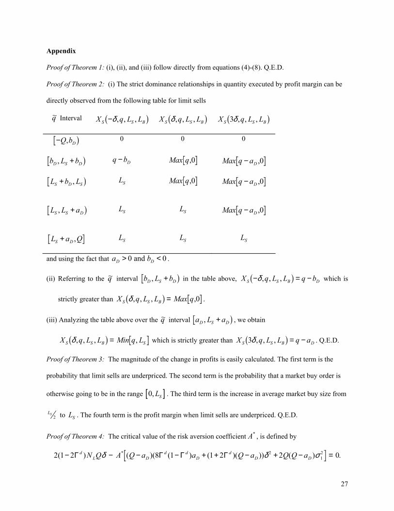
Proof of Theorem 2: (i) The strict dominance relationships in quantity executed by profit margin can be

directly observed from the following table for limit sells

~q Interval X q L LS S−δ, , ,b gB X q L LS Sδ, , ,b g B B X q L LS S3δ, , ,b g

−Q bD, g 0 0 0

b L bD S D, + g q bD− Max q,0 Max q aD− ,0

L b LS D S+ , g

LS Max q,0 Max q aD− ,0

L L aS S D, + g

LS LS Max q aD− ,0

L a QS D+ , LS LS LS

and using the fact that . a bD D> <0 0 and

(ii) Referring to the ~q interval b L bD S D, + g in the table above, which is

strictly greater than

X q L L qS S B− =δ, , ,b g bD−

X q L L Max qS S Bδ, , , ,b g = 0 .

(iii) Analyzing the table above over the ~q interval a L aD S D, + g , we obtain

X q L L Min q LS S Bδ, , , ,b g = S aD which is strictly greater than . Q.E.D. X q L L qS S B3δ, , ,b g = −

Proof of Theorem 3: The magnitude of the change in profits is easily calculated. The first term is the

probability that limit sells are underpriced. The second term is the probability that a market buy order is

otherwise going to be in the range [ ]0, SL . The third term is the increase in average market buy size from

2SL to . The fourth term is the profit margin when limit sells are underpriced. Q.E.D. SL

Proof of Theorem 4: The critical value of the risk aversion coefficient , is defined by A*

2 1 2 1 1 2 2 0212( ) ( )(8 ( ) ( )( )) ( ) .*− − − − + + − + −Γ Γ Γ Γd

L Dd d

Dd

D DN Q A Q a a Q a Q Q aδ δ =σ

27

Because the coefficient on is positive, if A* Γ d > 12 then <0 and the assumption > is satisfied

simply by the fact that risk aversion is positive.

A* A A*

First, consider the case: Γ di

i

QB

> ∑σδ

12

21

, which is equivalent to . Because the

condition is a maintained assumption,

Q cD< 2Γ a

QaD < Γ d > 12 in this case. For one calculates Lid = 0,

E W~ .02 = Computation yields

∂∂

δ δE WL

NQ

LQ a

QidL id

dD

~,2 2

= −LNMOQP +

− Γc h

which is strictly negative for positive . Hence Lid E W~2 is strictly negative for .

Because -A

L Q a NidD L∈ −( , / ]0 b g

Var W~2 /2 <0, the limit-order submitter’s utility (11) is maximized at the corner solution

. Lid = 0

Now consider the case Γ di

i

QB

< ∑σδ

12

21

, which is equivalent to Q . The first order

condition, i.e., FOC(L

a

σ

,

dD> 2Γ

id), is a cubic function with a positive third-order coefficient. The coefficients of

FOC are

c AN

c AN a Q Q Q

c A a Q N Q AQ

c N Q Q a

L

L Dd d

dD

dL

L Dd

33 2

22

12

12 2 2 2 2

12

0

6 7 1 2

8 2 2

2 2

=

= + − − +

= + − −

= −

δ

δ σ

δ δ

δ

,

( ) ( )

,

.

Γ Γ

Γ Γ

Γ

c he je jc h

Calculation provides the following results:

28

( ) ,

( ) ( ) ,

i Q a FOC L

ii FOC L Q qN

dD

id

id s

L

> ( =2 0

0

Γ ⇔

= − <L

) > 0

NMOQP

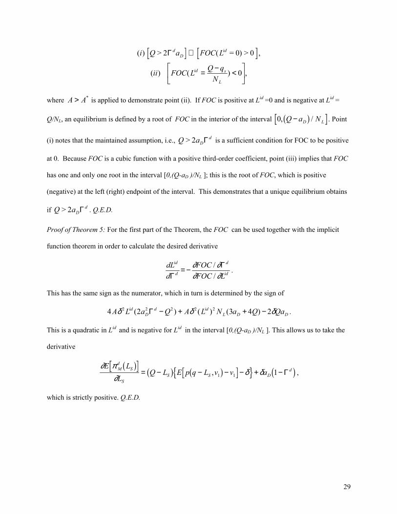
where is applied to demonstrate point (ii). If FOC is positive at LA A> * id =0 and is negative at Lid =

Q/NL, an equilibrium is defined by a root of FOC in the interior of the interval 0, /Q a ND−b g L . Point

(i) notes that the maintained assumption, i.e., is a sufficient condition for FOC to be positive

at 0. Because FOC is a cubic function with a positive third-order coefficient, point (iii) implies that FOC

has one and only one root in the interval [0,(Q-a

Q aDd> 2 Γ

D )/NL ]; this is the root of FOC, which is positive

(negative) at the left (right) endpoint of the interval. This demonstrates that a unique equilibrium obtains

if . Q.E.D. Q aDd> 2 Γ

Proof of Theorem 5: For the first part of the Theorem, the FOC can be used together with the implicit

function theorem in order to calculate the desired derivative

dLd

FOCFOC L

id

d

d

idΓΓ= − ∂ ∂

∂ ∂//

.

This has the same sign as the numerator, which in turn is determined by the sign of

4 2 3 4 22 2 2 2 2A L a Q A L N a Q QaidD

d idL Dδ δ( ) ( ) ( )Γ − + + − Dδ .

This is a quadratic in Lid and is negative for Lid in the interval [0,(Q-aD )/NL ]. This allows us to take the

derivative

∂ π∂

δ δE L

LQ L E p q L v v aM

dS

SS S D

db g b g b gn s c h= − − − − + −, 1 1 1 Γ ,

which is strictly positive. Q.E.D.

29

REFERENCES

Admati, A. R. and P. Pfleiderer, 1989, Divide and Conquer: A Theory of Intraday and Day-of-the-Week Mean Effects, Review of Financial Studies, 2, 189-223. Angel, 1992, Limit Versus Market Orders, Working Paper, Georgetown University. Bhattacharya, U. and M. Spiegel, 1991, Insiders, Outsiders, and Market Breakdowns, Review of Financial Studies, 4, 255-282. Black, F., 1971, Toward a Fully Automated Exchange, Financial Analysts Journal, July-August and November-December. Chakravarty, S. and C. Holden, 1995, An Integrated Model of Market and Limit Orders, The Journal of Financial Intermediation, 4, 213-241. Dutta, P. and A. Madhavan, 1997, Competition and Collusion in Dealer Markets, Journal of Finance, 52, 245-276. Easley, D. and M. O'Hara, 1987, Price, Trade Size, and Information in Securities Markets, Journal of Financial Economics, 19, 69-90. Easley, D. and M. O'Hara, 1991, Order Form and Information in Securities Markets, Journal of Finance 46, 905-927.

pstein, L., 1985, Decreasing Risk Aversion and Mean-Variance Analysis, Econometrica, 53, 945-961. E Foucault, T., 1999, Order Flow Composition and Trading Costs in a Dynamic Limit Order Market,

urnal of Financial Markets, 2, 99-134. Jo Glosten, L. R. and P. R. Milgrom, 1985, Bid, Ask, and Transaction Prices in a Specialist Market With

eterogeneously Informed Traders, Journal of Financial Economics, 14, 71-100. H Glosten, L. R., 1989, Insider Trading, Liquidity, and the Role of the Monopolist Specialist, Journal of

usiness 62, 211-235. B Glosten, L. R., 1994, “Is the Electronic Open Limit-Order Book Inevitable?” Journal of Finance, 49, 1127-161.

rossman, S. and M. Miller, 1988, Liquidity and Market Structure, Journal of Finance, 43, 617-633.

ence on Order ubmission Strategy, Journal of Financial and Quantitative Analysis, 31, 213-231.

al Dealer Pricing Under Transactions and Return Uncertainty, Journal of inancial Economics, 9, 47-73.

, 1999, NASDAQ Market Structure and Spread Patterns, Journal of Financial conomics, 45, 61-89.

1 G Harris, L. and J. Hasbrouck, 1996, Market Versus Limit Orders: The SuperDot EvidS Ho, T. and H. Stoll, 1981, OptimF Kandel, E. and L. MarxE

30

Kumar, P. and D. Seppi, 1993, Limit and Market Orders with Optimizing Traders, Working Paper,

negie Mellon University.

Econometrica, 53, 1315-1335.

, 1989, Informed Speculation with Imperfect Competition, Review of Economic Studies, 56, 17-356.

eland, H., 1992, Insider Trading: Should it be Prohibited?, Journal of Political Economy, 100, 859-887.

.H., 1991, Financial Innovations and Market Volatility, Blackwell Publishers, Cambridge, MA. 88pp.

he Microeconomics of Market Making, Journal of Financial and uantitative Analysis, 21, 361-376.

arlour, C., 1998, Price Dynamics in a Limit Order Market, Review of Financial Studies, 11, 789-816.

ock, K., 1990, The Specialist's Order Book and Price Anomalies, University of Chicago working paper.

asure of the Effective Bid-Ask Spread in an Efficient Market,

dity Provision with Limit Orders and a Strategic Specialist, Review of Financial

.

991, Risk Aversion, Market Liquidity, and Price Efficiency, Review of Financial

undaresan, S., 1989, Intertemporally Dependent Preferences and the Volatility of Consumption and

ohl, A. and S. Kandel, 1997, Implications of an Index-Contingent Trading Mechanism, Journal of

ohl, A., 1997, An Index-Contingent Trading Mechanism: Feasibility and Technical Implications, anagement Science, 43, 112-121.

Car Kyle, A. S., 1985, Continuous Auctions and Insider Trading, Kyle, A. S.3 L Miller, M2 O’Hara, M. and G. Oldfield, 1986, TQ P R Roll, R., 1984, A Simple Implicit MeJournal of Finance, 39, 1127-1139.

eppi, D., 1997, LiquiSStudies, 10, 103-150. Stoll, H., 1978, The Supply of Dealer Services in Securities Markets, Journal of Finance, 33, 1133-1151

ubrahmanyam, A., 1SStudies, 4, 417-441. SWealth, Review of Financial Studies, 2, 73-89. WBusiness, 70, 471-488. WM

31

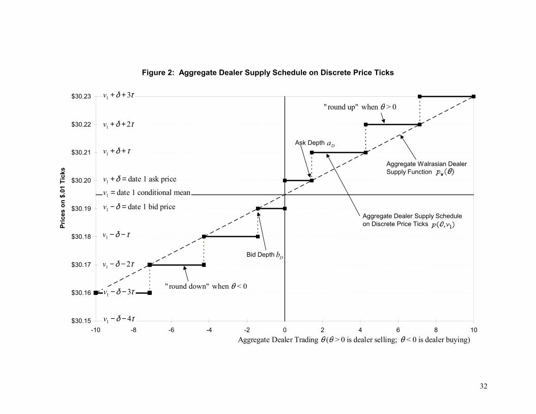
Figure 2: Aggregate Dealer Supply Schedule on Discrete Price Ticks

$30.15

$30.16

$30.17

$30.18

$30.19

$30.20

$30.21

$30.22

$30.23

-10 -8 -6 -4 -2 0 2 4 6 8 10

Pric

es o

n $.

01 T

icks

Ask Depth aD

Bid Depth bD

v1 + +δ τ

v1 2+ +δ τ

v1 3+ +δ τ

v1 − −δ τ

v1 2− −δ τ

v1 3− −δ τ

v1 4− −δ τ

Aggregate Walrasian DealerSupply Function

" round up" when > 0θ

" round down" when < 0θ

v1 + =δ date 1 ask price

v1 − =δ date 1 bid price

v1 = date 1 conditional mean

Aggregate Dealer Supply Scheduleon Discrete Price Ticks

Aggregate Dealer Trading ( > 0 is dealer selling; < 0 is dealer buying)θ θ θ

32

Figure 3: Aggregate Limit Sell Quantity Executed at a Negative ProfitMargin, a Normal Profit Margin, and a Windfall Gain Profit Margin

0

1

2

3

4

5

6

7

8

9

10

11

12

13

-14 -13 -12 -11 -10 -9 -8 -7 -6 -5 -4 -3 -2 -1 0 1 2 3 4 5 6 7 8 9 10 11 12 13 14

MB Quantity (q)

Agg

rega

te L

imit

Sell

Qua

ntity

Executed

Ask Depth aDBid De pth bD

Aggregate Limit Sell QuantityExecuted at a Negative Profit Margin (in Underpriced State)

Aggregate Limit Sell QuantityExecuted at a Normal Profit Margin (in Fairpriced State)

Aggregate Limit Sell QuantityExecuted at a Windfall Profit Margin (in Overpriced State)

Aggregate Limit Sell QuantityPicked Off by the Dealers at a Negative Profit Margin(in Underpriced State)

Aggregate Limit Sell Quantity Submitted 7SL =

33