decision analysis: part 2 bsad 30 dave novak source: anderson et al., 2013 quantitative methods for...
TRANSCRIPT

Decision analysis: part 2
BSAD 30
Dave Novak
Source: Anderson et al., 2013 Quantitative Methods for Business 12th edition – some slides are directly from J. Loucks © 2013 Cengage Learning
1

Overview
Risk analysisRisk profileSensitivity analysis
• Changes in states of nature• Changes in payoffs
EVPI calculation EOL calculation Building and using decision trees
2

Risk analysis
Risk analysis helps the decision maker recognize the difference between the expected value of a decision alternative, and the payoff that might actually occurRecall that a payoff is the result of a
combination of: 1) a decision alternative (you control this), and 2) a state of nature probability (you do not control this)
3

Risk analysis
The risk profile for a decision alternative shows the possible payoffs for the decision alternative along with their associated probabilitiesWe want to identify the probability or
likelihood that a particular payoff will occurBasically, we want to list out ALL possible
payoffs, and their probabilities of occurrence
4

PDC example - lecture 15 Payoff table with P(s1) = 0.8 and P(s2) = 0.2
PAYOFF TABLE States of Nature Strong Demand Weak Demand
Decision Alternative s1 s2
Small complex, d1 8 7
Medium complex, d2 14 5
Large complex, d3 20 -9
5

PDC example – lecture 15
1
.8
.2
.8
.2
.8
.2
d1
d2
d3
s1
s1
s1
s2
s2
s2
Payoffs
$8 mil
$7 mil
$14 mil
$5 mil
$20 mil
-$9 mil
2
3
4
6

PDC example - lecture 15
1
small d1
medium d2
large d3
2
3
4
7

Risk profile
d3 (90 unit) decision alternative versus d2 (60 unit) decision alternative
8
9
.20
.40
.60
.80
1.00
-10 -5 0 5 10 15 20
Pro
bab
ility
11
.20
.40
.60
.80
1.00
-10 -5 0 5 10 15 20
Pro
bab
ility

Value of perfect information
Calculate EV assuming MOST OPTIMISTIC payoff for both states of nature (does not need to be the same decision) = EVwPI
Take the EV associated with your decision (this is the largest EV value across all decisions) = EVwoPIGiven imperfect information, this is what we
would choose to do
9

Value of perfect information
EVPI =
EVPI =
EVPI =
10

Expected opportunity loss
Using the regret table from lecture #15, we can calculate “the expected opportunity lost” (EOL) associated with each decision
11
REGRET TABLE States of Nature
Strong Demand Weak Demand
Decision Alternative s1 s2
Small complex, d1 12 0 Medium complex, d2 6 2 Large complex, d3 0 16
Expected opportunity loss
12

Expected opportunity loss
The minimum of the EOL values always provides the optimal decision
Notice that EVPI = Expected Opportunity Loss (EOL) for decision d3 (90 units)
EVPI is ALWAYS equal to the EOL for the optimal decision
13

Sensitivity analysis
Sensitivity analysis can be used to determine how changes to the following inputs affect the recommended decision alternative:probabilities for the states of nature can be
subjective, and therefore subject to changevalues of the payoffs
14

Sensitivity analysis
If a small change in the value of one of the inputs (state of nature probabilities or payoff values) causes a change in the recommended decision alternative, extra effort and care should be taken in estimating the input value
If changes to inputs do not really impact your decision, you can feel more confident about this decision
15

Sensitivity analysis
One way to address the sensitivity question is to select different values for either the state of nature probabilities or the payoff values, and then do some “what if” calculations
Say we flip our state of nature probabilities for the PDC problem…
16

Modified PDC example
1
.2
.8
.2
.8
.2
.8
d1
d2
d3
s1
s1
s1
s2
s2
s2
Payoffs
$8 mil
$7 mil
$14 mil
$5 mil
$20 mil
-$9 mil
2
3
4
17

Modified PDC example
1
small d1
medium d2
large d3
2
3
4
18

Modified PDC example
1
.5
.5
.5
.5
.5
.5
d1
d2
d3
s1
s1
s1
s2
s2
s2
Payoffs
$8 mil
$7 mil
$14 mil
$5 mil
$20 mil
-$9 mil
2
3
4
19

Modified PDC example
1
small d1
medium d2
large d3
2
3
4
20

EV comparison

Graphing for 2 state of nature problem Like a LP with two decision variables, if we
only have two states of nature, we can perform sensitivity analysis graphically
Generalize relationship for P(s1) and P(s2)
22

EV calculations for decision variables
23
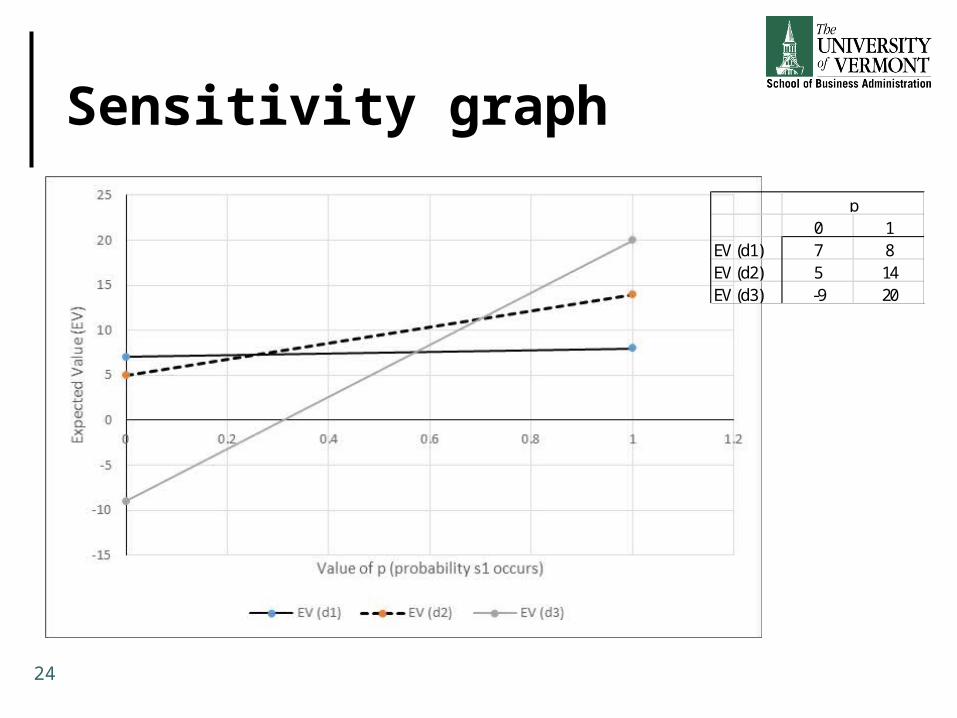
Sensitivity graph
24
0 1EV (d1) 7 8EV (d2) 5 14EV (d3) -9 20
p

Sensitivity graph
25
d1 provides highest EV
d2 provides highest EV
d3 provides highest EV
0 1EV (d1) 7 8EV (d2) 5 14EV (d3) -9 20
p
Solve for eachintersection point way we solved for internal points in LP
Set two linear equationsequal to one anotherand solve for p

Solving for inflection points
26
Intersection of EV(d1) and EV(d2) linesEV(d1) = p + 7
EV(d2) = 9p + 5
So, p + 7 = 9p + 5 2 = 8p p = = 0.25

Solving for inflection points
27
Intersection of EV(d2) and EV(d3) linesEV(d2) = 9p + 5
EV(d3) = 2p - 9
So, 9p + 5 = 29p - 9 14 = 20p p = = = 0.7

Sensitivity graph
28
d1 provides highest EV
d2 provides highest EV
d3 provides highest EV
p = 0.25 p = 0.7

What are managerial implications?
29
If probability of strong demand, P(s1) < 0.25, then choose d1 (30 units)
If probability of strong demand, P(s1) = 0.25, then choose either d1 (30 units) or d2 (60 units)
If probability of strong demand, 0.25 < P(s1) < 0.7, then choose d2 (60 units)
If probability of strong demand, P(s1) = 0.7, then choose either d2 (60 units) or d3 (90 units)
If probability of strong demand, P(s1) > 7 then choose d3 (90 units)

What about changes in payoff values?
30
From the PDC problem, we have:EV(d1) = 7.8
EV(d2) = 12.2
EV(d3) = 14.2
So, we conclude that building 90 units is the optimal decision (d3) as long as EV(d3) ≥ 12.2

What about changes in payoff values?
31
Let’s look at changing one of the payoff values for decision alternative d3 (90 units)
Hold the state of nature probabilities constant for both s1 (strong demand) and s2
(weak demand)P(s1) = 0.8, and P(s2) = 0.2
Let S = payoff value for d3 assuming s1W= payoff value for d3 assuming s2

What about changes in payoff values?
32
We can write EV(d3) as:
Examine a change in one of the payoff values for a particular decision alternativeHere, we will hold payoff for weak demand
constant at -9

What about changes in payoff values?
33
Solve for S0.8S – 1.8 ≥ 12.20.8S ≥ 14S ≥ 17.5
What does this mean?As long as our original state of nature
probabilities hold, we should build d3, as long as the payoff under the strong demand scenario is ≥ 17.5 mil

What about changes in payoff values?
34
Examine a change in the other payoff value for decision alternative d3
we will hold payoff for strong demand constant at 20, and investigate changes in weak demand

What about changes in payoff values?
35
Solve for W16 + 0.2W ≥ 12.20.2W ≥ -3.8W ≥ -19
What does this mean?As long as our original state of nature
probabilities hold, we should build d3, as long as the payoff under the weak demand scenario is ≥ -19 mil

What about changes in payoff values?
36
When we hold the state of nature probabilities constant at P(s1) = 0.8, and P(s2) = 0.2, the d3 decision does not seem to be particularly sensitive to variations in the payoff
Why?Probability that demand is strong, P(s1), is
very high AND expected payoff is very highUsing the EV approach, this combination
leads us to choose d3

Decision trees
37
Just a graphical representation of the decision-making processShows a progression over time
Squares: decision nodes that we control Circles: chance nodes that we do not
control

Decision tree
1
.8
.2
.8
.2
.8
.2
d1-build 30 units
s1
s1
s1
s2
s2
s2
Payoffs
$8 mil
$7 mil
$14 mil
$5 mil
$20 mil
-$9 mil
2
3
4
38
d2-build 60 units
d3-build 90 units
Given each decision, we are then subject to demand, which we cannot control
For each decision alternativeand state of nature pair, we have an expected payoff

Decision trees
39
Hemmingway, Inc., is considering a $5 million research and development (R&D) project. Profit projections appear promising, but Hemmingway's president is concerned because the probability that the R&D project will be successful is only 0.50.
Furthermore, the president knows that even if the project is successful, it will require that the company build a new production facility at a cost of $20 million in order to manufacture the product.

Decision trees
40
If the facility is built, uncertainty remains about the demand and thus uncertainty about the profit that will be realized.
Another option is that if the R&D project is successful, the company could sell the rights to the product for an estimated $25 million. Under this option, the company would not build the $20 million production facility.

Decision trees
41
Identify the “pieces” or nodes associated with this problem
We have to present this information in a time dependent sequence of events

Decision trees
42
1. Make a decision whether to start the R&D project or not
a) Start R&D project (cost of $5 mil) proceed
b) Do not start R&D project (cost of zero) stop

Decision trees
43

Decision trees
44
2. If we start R&D, there is a state of nature or chance event that the project will be successful, where:
a) P(R&D success) = 0.5 proceed
b) P(R&D failure) = 0.5 stop and lose $5 mil

Decision trees
45

Decision trees
46
3. If R&D is successful, we make a decision whether to:
a) Build the production facility (cost of $20 mil) proceed
b) Sell the rights to the product for $20 mil stop

Decision trees
47
Decision trees
48
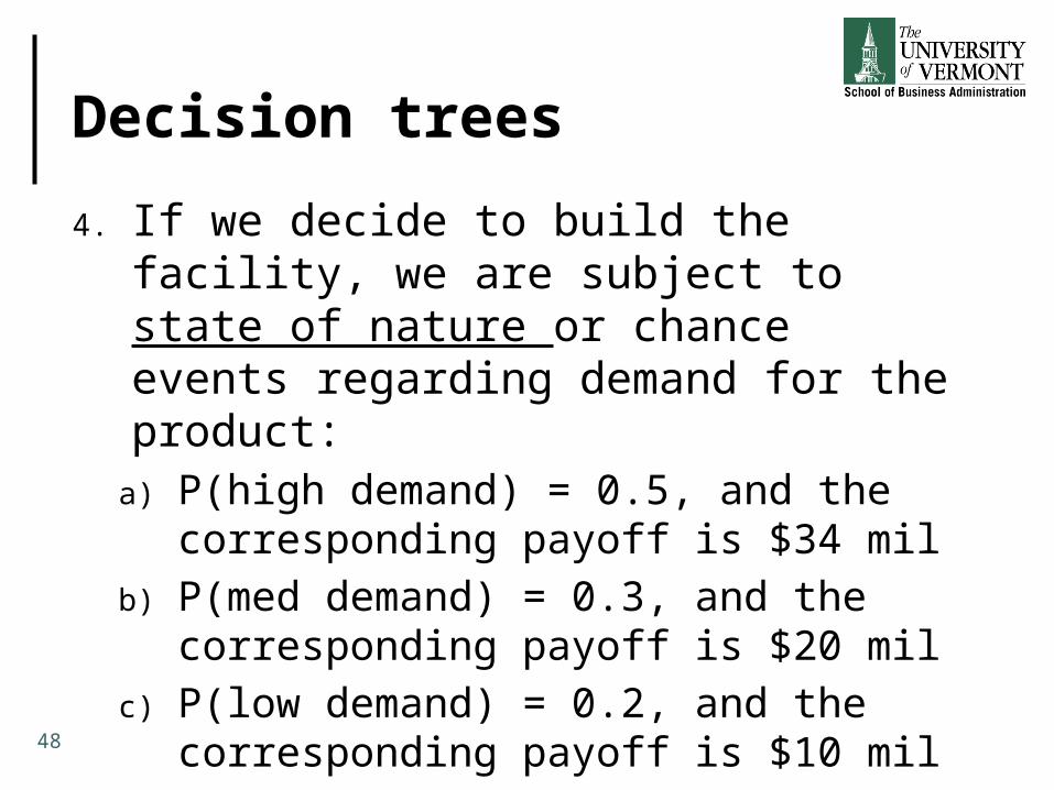
4. If we decide to build the facility, we are subject to state of nature or chance events regarding demand for the product:
a) P(high demand) = 0.5, and the corresponding payoff is $34 mil
b) P(med demand) = 0.3, and the corresponding payoff is $20 mil
c) P(low demand) = 0.2, and the corresponding payoff is $10 mil

Decision tree

Decision trees
50
Populate the decision tree with probabilities, so we can calculate EV for different scenarios
We work BACKWARDS to calculate EV for each chance or state of nature nodeEV (node 4)EV (node 2)

Decision trees
51

Decision tree

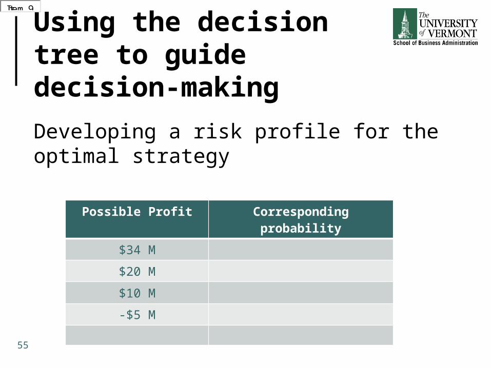
Using the decision tree to guide decision-making
53
Should the company undertake the R&D project?
If R&D is successful, what should company do, sell or build?

Using the decision tree to guide decision-making
54
What is EV of your decision strategy?
What would selling price need to be for company to consider selling?
What about for recovering R&D cost?
Using the decision tree to guide decision-making
55
Developing a risk profile for the optimal strategy
Possible Profit Corresponding probability
$34 M
$20 M
$10 M
-$5 M
Item 5Item 6Item 7Item 8Item 9Item 5Item 6Item 7Item 8Item 9

What would the payoff table look like?
56
PAYOFF TABLE States of Nature
High Demand Med Demand Low Demand
Decision Alternatives
Build
Sell
34 20 10
20 20 20

What would the regret table look like?
57
REGRET TABLE States of Nature
High Demand Med Demand Low Demand
Decision Alternatives
Build
Sell
0 0 10
14 0 0

Value of perfect information
EVwPI =
EVwoPI =
EVPI =
58
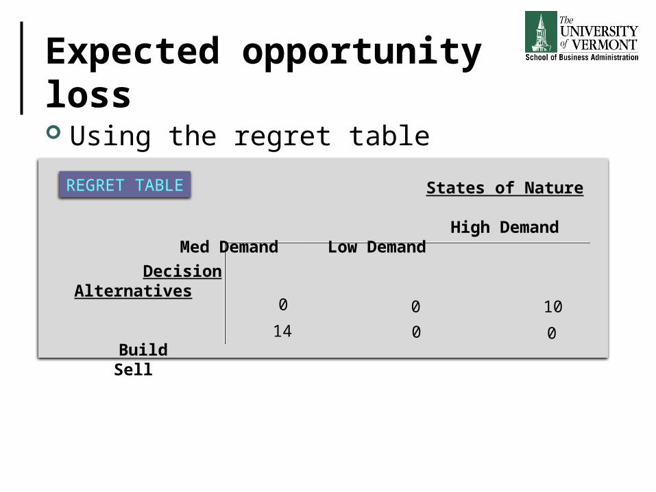
Expected opportunity loss
Using the regret table
REGRET TABLE States of Nature
High Demand Med Demand Low Demand
Decision Alternatives
Build
Sell
0 0 10
14 0 0

Summary
Risk analysisRisk profileSensitivity analysis
• Changes in states of nature• Changes in payoffs
EVPI calculation EOL calculation Building and using decision trees
60