decision support for multi-objective linear programming using an … · 2020. 4. 2. · or...
TRANSCRIPT

Decision support for multi-objective linearprogramming using an interactive graphic presentation.
Item Type text; Dissertation-Reproduction (electronic)
Authors Anderson, Russell Kay.
Publisher The University of Arizona.
Rights Copyright © is held by the author. Digital access to this materialis made possible by the University Libraries, University of Arizona.Further transmission, reproduction or presentation (such aspublic display or performance) of protected items is prohibitedexcept with permission of the author.
Download date 07/08/2021 14:08:19
Link to Item http://hdl.handle.net/10150/186950

INFORMATION TO USERS
This manuscript has been reproduced from the microfilm master. UMI
films the text directly from the original or copy submitted. Thus, some
thesis and dissertation copies are in typewriter face, while others may
be from any type of computer printer.
The quality of this reproduction is dependent upon the quality of the
copy submitted. Broken or indistinct print, colored or poor qUality
illustrations and photographs, print bleedtbrough, substandard margins,
and improper alignment can adversely affect reproduction.
In the unlikely event that the author did not send UMI a complete
manuscript and there are missing pages, these will be noted. Also, if
unauthorized copyright material had to be removed, a note will indicate
the deletion.
Oversize materials (e.g., maps, drawings, charts) are reproduced by
sectioning the original, beginning at the upper left-hand comer and
continuing from left to right in equal sections with small overlaps. Each
original is also photographed in one exposure and is included in
reduced form at the back of the book.
Photographs included in the original manuscript have been reproduced
xerographically in this copy. Higher quality 6" x 9" black and white
photographic prints are available for any photographs or illustrations
appearing in this copy for an additional charge. Contact UMI directly
to order.
A Bell & Howell Information Company 300 North Zeeb Road. Ann Arbor. MI 48106·1346 USA
313!761·4700 800:521·0600


Order Number 9517562
Decision support for multi-objective linear programming using an interactive graphic presentation
Anderson, Russell Kay, Ph.D.
The University of Arizona, 1994
Copyright ©1994 by Anderson, Russell Kay. All rights reserved.
V·M·X 300 N. Zeeb Rd. Ann Arbor, MI 48106


DECISION SUPPORT FOR
MULTI-OBJECTIVE LINEAR PROGRAMMING
USING AN INTERACTIVE GRAPHIC PRESENTATION
by
Russell Kay Anderson
Copyright © Russell Kay Anderson
A Dissertation Submitted to the Faculty of the
DEPARTMENT OF MANAGEMENT INFORMATION SYSTEMS
In Partial Fulfillment of the Requirements For the Degree of
DOCTOR OF PHILOSOPHY WITH A MAJOR IN MANAGEMENT
I n the Grad uate College
THE UNIVERSITY OF ARIZONA
1 994

THE UNIVERSITY OF ARIZONA GRADUATE COLLEGE
2
As members of the Final Examination Committee, we certify that we have
read the dissertation prepared by ____ R_u_s_s_e_l~l __ Ka~y_A~nd_e_r_s_o~n~ ____________ ___
entitled DECISION SUPPORT FOR MULTI-OBJECTIVE LINEAR PROGRAMMING ---------------------------------------------------------------USING AN INTERACTIVE GRAPHIC PRESENTATION
and recommend that it be accepted as fulfilling the dissertation
requirement for the Degree of
D*] , '2 SIB, 'f ~!.....f-!-~-t-f--'- Lj
Date
Final approval and acceptance of this dissertation is contingent upon the candidate's submission of the final copy of the dissertation to the Graduate College.
I hereby certify that I have read this dissertation prepared under my direction and recommend that it be accepted as fulfilling the dissertation

3
STATEMENT BY AUTHOR
This dissertation has been submitted in partial fulfillment of requirements for an advanced degree at The University of Arizona and is deposited in the University Library to be made available to borrowers under rules of the Library.
Brief quotations from this dissertation are allowable without special permission, provided that accurate acknowledgment of source is made. Requests for permission for extended quotation from or reproduction of this manuscript in whole or in part may be granted by the copyright holder.

4
ACKNOWLEDGEMENTS
Many people have made significant contributions toward the completion of
this dissertation. I would like to thank my dissertation co-advisors, Olivia R. Liu
Sheng and Moshe Dror for their careful and thoughtful reviews and suggestions;
my wife Charmaine for enduring seven years of frequent moves, reduced income,
and a stressful husband; and my children Jacob, Kimberly, Ryan, Sara, Jed, and
John for their patience and their eagerness to test and crash the software during
development.

5
TABLE OF CONTENTS
LIST OF ILLUSTRATIONS ............................... 11
LIST OF TABLES ...................................... 13
ABSTRACT . . . . . . . . . . . . . . . . . . . . . . . . . . . . . . . . . . . . . . . . . .. 14
1. INTRODUCTION ................................... 16
1.1 Linear Programming and Optimization. . . . . . . . . . . . . . . .. 16
1.2 Research Objectives. . . . . . . . . . . . . . . . . . . . . . . . . . . . .. 17
1.3 Research Questions .............................. 18
1.4 Overview of Dissertation .......................... 19
2. MCDM LITERATURE REVIEW. . . . . . . . . . . . . . . . . . . . . . . . .. 22
2.1 The Mathematical Formulation of Linear Programming. . . . .. 22
2.2 Multi-Objective Linear Programming . . . . . . . . . . . . . . . . .. 23
2.3 The Vocabulary and Concepts of LP and MOLP .......... 24
2.4 The Simplex Methodology ......................... 35
2.5 Algorithms Specific to MOLP .. . . . . . . . . . . . . . . . . . . . .. 38
2.6 A Review of MCDM ............................. 41
2.6.1 Value and Utility. . . . . . . . . . . . . . . . . . . . . . . . .. 44
2.6.2 MCDM Methodology Evaluation . . . . . . . . . . . . . .. 45
2.7 Review of MCDM Methodologies .................... 48

6
TABLE OF CONTENTS - continued
2.7.1 Feasible Region Reduction ................... 49
2.7.2 Feasible Direction (Line Search) ............... 52
2.7.3 Criterion Weighting. . . . . . . . . . . . . . . . . . . . . . .. 56
2.7.4 Surrogate Worth Trade-off. . . . . . . . . . . . . . . . . .. 58
2.7.5 Visual Interactive ......................... 61
2.7.6 The Dror-Gass Methodology. . . . . . . . . . . . . . . . .. 63
2.7.7 Conclusion. . . . . . . . . . . . . . . . . . . . . . . . . . . . .. 64
3. DECISION THEORY ................................. 66
3.1 Introduction to Decision Rules ...................... 66
3.2 Proper Application of Weak Orders ................... 69
4. MOLP METHODOLOGY .............................. 73
4.1 Assumptions About the MOLP Model ................. 73
4.2 Assumptions About the Decision Maker ................ 73
4.3 Strategy to Solve the Problem ....... . . . . . . . . . . . . . . .. 74
4.4 Description of the Algorithm ....................... 76
4.4.1 The OM's Preferences ...................... 76
4.4.2 Locating an Initial Efficient Solution ............ 78
4.4.3 The Interactive Process. . . . . . . . . . . . . . . . . . . . .. 85
4.4.4 Move to Next Solution. . . . . . . . . . . . . . . . . . . . .. 85

7
TABLE OF CONTENTS - continued
4.4.5 Selecting a PREFERRED Solution .............. 88
4.4.6 Finding a Compromise Solution When Cycling ..... 90
4.5 Methodology Objectives. . . . . . . . . . . . . . . . . . . . . . . . . .. 93
4.6 Discussion of the Proposed Methodology ............... 95
4.6.1 Variable Preference Refinement. . . . . . . . . . . . . . .. 96
4.6.2 Locating Initial Solution. . . . . . . . . . . . . . . . . . . .. 97
4.6.3 Breaking the Tie Between Solutions of Equal RANK .. 101
4.6.4 The Interactive Exploration Process ............. 103
4.6.5 Computing the Compromise Solution ............ 104
5. DESIGN OF THE MOLP DATA STRUCTURES ............... 105
5.1 Introduction ................................... 105
5.2 MOLP Problem Characteristics ...................... 105
5.3 Operating Environment ........................... 108
5.4 Analysis and Design .............................. 110
5.5 MOLP Entity-Relationship Diagram ................... 112
5.6 Conversion From ER Diagram to Minimal Logical Record Structure .............................. 116
5.7 Selection of the Data Structures ..................... 117
5.8 Modifications to Support Large Problems ............... 123

8
TABLE OF CONTENTS - continued
5.9 Evaluation of the Methodology ...................... 129
6. DESIGN OF THE MOLP INTERFACE AND SOLUTION PRESENTATION .................................. 132
6.1 Definition of Visualization ......................... 132
6.2 Rationale for the Use of Visualizations ................. 133
6.3 Problems With Visualization Experimentation ............ 136
6.4 Factors of Visualization Performance .................. 138
6.4.1 Data Attributes 139
6.4.2 Task Attributes 139
6.4.3 User Attributes 140
6.4.4 Visualizations ............................ 140
6.5 Commentary on Previous Research .................... 150
6.6 Direct Manipulation ............................. 151
6.7 Design of Exploration Subsystem and Solution Visualization 153
6.7.1 Characteristics of the Efficient Solution Exploration Data ........ . 155
6.7.2 The Solution Exploration Task . 157
6.7.3 User Interface Requirements ... 158
6.7.4 Design of the Exploration Process .............. 159
6.8 The Solution Views .............................. 159

9
TABLE OF CONTENTS - continued
6.8.1 Exploration History Map .................... 160
6.8.2 Single Solution Objective Wheel ............... 162
6.8.3 Two Solution Objective Wheel ................ 164
6.8.4 Single and Multi-Solution Bar Graphs ........... 165
6.8.5 Line Graph .............................. 167
6.8.6 Multi-Solution Color Stacks .................. 168
6.8.7 Single and Multi-Solution Text Lists ............ 170
6.8.8 Issues of Design Common to More Than One View .. 173
6.8.9 Coding of the Solution Views 176
6.9 Design of the Preference Specification ................. 179
7. SOFTWARE EVALUATION ............................. 185
7.1 Test Design ................................... 185
7.2 Test Plan ..................................... 188
7.3 The Pilot Test ................................. 190
7.4 Results of the Pilot Test ........................... 192
7.5 Test Administration .............................. 193
7.6 Test Results ................................... 194
7.7 Other Observations .............................. 208
7.8 "Real World" Evaluation .......................... 210

10
TABLE OF CONTENTS - continued
7.9 Summary of Test Results .......................... 212
7.10 Future Investigations ............................ 215
8. SUMMARy ......................................... 218
8.1 Research Objectives .............................. 218
8.2 Research Results ................................ 219
8.2.1 Modifications of the Methodology .............. 219
8.2.2 The Methodology With Respect to Decision Theory .. 220
8.2.3 Design for Large Problems ................... 221
8.2.4 The Solution Presentation .................... 222
8.2.5 Software Testing .......................... 223
8.3 Recommendations for Future Research ................. 225
APPENDIX A: PRE-TEST QUESTIONNAIRE .................. 228
APPENDIX B: TUTORIAL FOR WALL PROBLEM ............... 231
APPENDIX C: TASK DEFINITION FOR WALL PROBLEM ........ 234
APPENDIX D: EVALUATION OF WALL PROBLEM ............. 235
APPENDIX E: TUTORIAL FOR MOLP PROBLEM .............. 238
APPENDIX F: TASK DEFINITION FOR MOLP PROBLEM ........ 246
APPENDIX G: EVALUATION OF MOLP PROBLEM ............. 248
REFERENCES ......................................... 252

11
LIST OF ILLUSTRATIONS
FIGURE 2-1 LP problem graphic representation .................. 25
FIGURE 2-2 Minimization LP graphic representation. . . . . . . . . . . . . .. 27
FIGURE 2-3 LP problem with varying objective levels .............. 28
FIGURE 2-4 LP problem second objective ...................... 30
FIGURE 2-5 LP problem with two objectives .................... 32
FIGURE 2-6 LP problem with dominated objective ideal ............ 34
FIGURE 2-7 MCDM taxonomy ............................. 43
FIGURE 4-1 The MOLP system . . . . . . . . . . . . . . . . . . . . . . . . . . . .. 77
FI G URE 4-2 Refinement of the weak order on variables ... . . . . . . . . .. 79
FIGURE 4-3 Refinement of a variable indifference set .............. 80
FIGURE 4-4 Locating the initial solution. . . . . . . . . . . . . . . . . . . . . .. 82
FIGURE 4-5 A preferred solution ............................ 84
FIGURE 4-6 Locating the next solution . . . . . . . . . . . . . . . . . . . . . . .. 86
FIGURE 4-7 An objective's ideal and minimum values . . . . . . . . . . . . .. 90
FIGURE 5-1 MOLP entity-relationship diagram .................. 113
FIGURE 5-2 MOLP minimal logical record structure ............... 118
FIGURE 5-3 MOLP object class diagram ....................... 124
FIGURE 5-4 Expanded entity-relationship diagram for decision variables . 126

12
LIST OF ILLUSTRATIONS - continued
FIGURE 5-5 Expanded minimal logical record structure for decision variables .............................. 127
FIGURE 6-1 Visualization of sum game ........................ 135
FIGURE 6-2 Kiviat charts ................................. 143
FIGURE 6-3 The solution map .............................. 161
FIGURE 6-4 Single solution objective wheel ..................... 163
FIGURE 6-5 Two solution objective wheel ...................... 164
FIGURE 6-6 Single solution bar graph ......................... 166
FIGURE 6-7 Multi-solution bar graph ......................... 166
FIGURE 6-8 Line graph with point readings ..................... 168
FIGURE 6-9 Multi-solution color stacks with value readings .......... 170
FIGURE 6-10 Single solution text list 171
FIGURE 6-11 Multi-solution text list 172
FIGURE 6-12 Graph range options ........................... 174
FIGURE 6-13 Solution view inheritance hierarchy ................. 178
FIGURE 6-14 Preference wall ............................... 181

13
LIST OF TABLES
TABLE 7-1 Usefulness and ease of use of preference wall functions 195
TABLE 7-2 Overall assessment of preference wall .................. 196
TABLE 7-3 Effectiveness of solution views ...................... 203
TABLE 7-4 Effectiveness and satisfaction with MOLP software ........ 207
14
ABSTRACT
Many decisions in real world applications are based on conflicting criteria
or objectives. In order to improve one objective, it is necessary to sacrifice
another. Linear programming has long been used to optimize a single objective.
When a linear programming problem involves multiple objectives (MOLP), it is
usually not possible to locate a single solution that simultaneously optimizes all
objectives. Hence, a methodology is needed to help the decision maker (DM)
explore the space of feasible solutions in order to locate an acceptable compromise
solution.
An interactive approach that supports the DM in the exploration process is
presented. The methodology is implemented on a microcomputer running a
graphical user interface. The computations are based on an expansion of the Dror
Gass [1987] methodology in which candidate solutions are located using weak
order preferences for variables and objectives. It differs from previous
methodologies in that it does not require burdensome trade-off ratios or strength
of preference comparisons.
During exploration, the OM is presented a multi-faceted graphical
representation of solutions for consideration. Previous studies of the effectiveness
of graphics to support the decision making process have used static presentations

15
of the data. The graphic presentation as implemented is dynamic. It makes use
of animation, interactive zoom (or inspect), and interactive highlighting of the
results to improve its effectiveness. In the design of the interface, special attention
was paid to the requirements for supporting interaction with large LP problems.
The software implementation and methodology were tested by subjects
drawn from faculty and students at the University of Arizona. It was also reviewed
in industry. The results are presented.

16
Chapter 1 - Introduction
1.1 Linear Programming and Optimization
Linear PI'ogl'amming (LP) is a problem formulation methodology by which
an optimal solution (maximum or minimum) to a linear function (the objective)
is located. LP problems were first formulated in 1939 by L. V. Kantorovich, a
Soviet mathematician, but his work remained unknown to the Western world until
1959. In 1947, George P. Dantzig, while working as an adviser to the United
States Air Force independently reformulated the problem. In 1949 he published
a method for solving LP problems. This method, which he called the "simplex
method", is still in use today. [Bazarra 1977]
Linear programming methodology was designed [0 locate the optimal
solution to a single linear objective function. Yet, frequently in a decision making
situation, the decision maker (OM) is faced with not one but many objectives to
be optimized concurrently. For example, in a business environment one objective
may be to maximize profit while a second objective may be [0 maximize market
share. While it is possible, it is not likely that the solution optimizing the first
objective also optimizes the second objective, nor does the solution optimizing the
second objective optimize the first objective. Hence, the critical difference

17
between single and multiple objective linear progl'amming (MOLP) - in MOLP
no single solution is likely to optimize all objectives.
The task of locating a "best" solution in MOLP is not simply a matter of
computation as it is with its single-objective counterpart. Since no single solution
is likely to optimize all objectives, either the optimizing solution of a single
objective must be chosen (giving up optimality on the other objectives) or a
compromise solution is chosen which may not achieve optimality for any single
objective, but doesn't totally sacrifice attainment of one objective in order to
achieve optimality on another.
1.2 Research Objectives
The goal of the work described herein is to refine the methodology and
study the workability of the Oror-Gass [1987] approach to MOLP when employed
as the underlying methodology in the design of a MOLP decision support system
(OSS). The necessary refinements, which became apparent in a previous
implementation of the methodology [Oror, Shoval, and Yellin 1991], include a way
to break ties in the selection of adjacent candidate solutions, and a way to handle
cycling in the search process.
The study is in three parts: first, the evaluation of the methodology with
respect to mathematically based decision theory; second, the study of how best to

18
implement the user interface and presentation of results, particularly with respect
to handling large data sets; and third, the evaluation of the effectiveness of the
methodology and its implementation in a MOLP problem solving environment.
To be able to fully evaluate the methodology, a workable implementation is
needed. That implementation must be complete and easy to use, yet able to
manipulate and clearly present the solutions to large MOLP problems. The
development of such a system is expected to be the major effort of the project.
To accomplish the above mentioned requirements, it was decided at the
outset, that as much as possible, all results would be presented graphically using
the recent developments in data presentation from the field of scientific
visualization. It was also decided that the user interaction would employ the
concepts of dil'ect manipulation as introduced by Schneidermann [1983].
Scientific visualization is a discipline in which methods are studied to visually
represent large volumes of data. Direct manipulation is a concept in computer
human interaction in which the objects with which the user is working, (either
tangible or intangible) are manipulated directly on the computer video display
unit.
1.3 Research Questions
The above described research goals lead to the following research qeustions:

19
1. How can the Dror-Gasss methodology be refined in order to overcome its known shortcomings?
a) How should ties be resolved when selecting from adjacent candidate solutions?
b) How should solutions be located after detecting cycling in the search process.
2. How should the interface with the decision maker be implemented in order to facilitate the workability of the methodology?
a) What is the best way to present and manipulate large problems with high variable and constraint counts?
b) What data structures are needed to efficiently and effectively support processing of large problems?
c) Will a graphic presentation of the results facilitate decision maker comprehension and evaluation of the possible solutions?
3. What is the workability of the Dror-Gass methdology?
a) How consistent is the methodology with respect to existing mathematically based decision theory?
b) How effective is the methodology and the resulting implementation in a MOLP decision making environment?
1.4 Overview of Dissertation
MOLP is part of a larger field of study called Multi-Criteria Decision
Making (MCDM). Chapter 2 contains an overview of the methodologies and
mathematics of MCDM. I t first presents the definitions and mathematics of linear
programming, focusing on those theorems and procedures employed in the MOLP

20
system presented herein. Following this, a review of previous and current work in
MCDM is presented. The relationship of MOLP to MCDM is first described.
Then a review of DSS's designed to be used in MCDM is made. The good and the
bad aspects of various systems are discussed.
Chapter 3 presents the axioms and theories by which the proposed system
is designed and justified. It is done from a mathematical perspective.
Chapter 4 presents in detail the design objectives of the proposed system
and a description of the algorithm underlying the proposed system, including any
necessary refinements of the Dror-Gass algorithm. This is followed by a discussion
of the algorithm, describing how each step is justified axiomatically in terms of the
theory presented in chapter 3.
Chapter 5 discusses the design of the data structures required to support
large MOLP problems. The structures were designed as objects for
implementation using an object-oriented development environment. The primary
methodology employed was an adaptation of a database design methodology
proposed by Hawryszkiewycz [1991].
The design of the visualizations used in the software is described in Chapter
6. It begins with a review of the scientific visualization and presentation graphics
literature. This is followed by a description of the graphics implemented in the
system and a discllssion of their rationale.

21
Chapter 7 presents the software evaluation, including the test plan,
administration, and results. It concludes with a discussion of how well the
software meets the original design objectives as assessed by the testing.
Chapter 8 summarizes the findings of the dissertation research. It also
concludes with recommendations for future enhancement and evaluation of the
software, and modification of the underlying methodology.

Chapter 2 - MCDM Literature Review
2.1 The Mathematical Formulation of Linear Programming
A LP problem may be expressed mathemadcally as:
Maximize ClxI + cr2 + ... + C,;X"
Subject to
anxI + alr2 + ... + all;x" ::; bI a21 x 1 + a22x2 + ... + a2nxn ::; b2
amlxI + amr2 + ... + am,;X" ::; bm Xl' X2, ... X,,;:: 0
22
Note that an objective to be minimized may be stated as a maximization problem
by reversing the signs of the objective function coefficients and that the constraint
set may also include equalities. The same problem is conveniently expressed using
matrix notadon as:
Maximize ex
Subject to
Ax::; b x ~ 0
where e is a row vector of dimension n, x and b are column vectors of dimension
nand m respecdveiy, and A is an m by n matrix.
The representation of a LP problem is restricted in a number of ways. First,
as already mentioned, the objective must be expressed as a linear function of the
"decision variables". Thus, interactions between the variables are not allowed and

23
allowed and the contribution of each decision variable to the objective is at a
constant rate. Second, the range of the decision variables used to satisfy the
objective is restricted by a set of linear equalities and/or inequalities, which form
the constraint set of the problem. Note that the same restriction of linearity also
applies to the constraints. Third, LP makes the assumption that all decision
variables are real-valued continuous quantities. The method may not produce an
optimal solution in which whole numbered values are required. For example, if
LP is applied to a production problem in which one of the decision variables is the
number of cars to produce, it is possible that the LP solution may be 18.63 cars,
which for practical purposes is not possible. Fourth, the assumption is made that
the constant values (coefficients) used in defining the objective function and the
constraints are known with certainty. There is no provision allowing some of the
constants to be treated as random variables and evaluated using probability and
statistical decision theory. A final assumption is that all decision variable values
are non-negative, which is not a problem since unrestricted variables may be
represented as a combination of non-negative variables.
2.2 Multi-Objective Linear Programming
When translated into a linear programming problem, the single objective
function is replaced by a set of objective functions. In the matrix notation
presented above, the coefficient vector c is replaced by a k by 1l matrix of

24
coefficients C, where each of the k rows in C corresponds to one of the objectives
to be optimized.
2.3 The Vocabulary and Concepts of LP and MOLP
This section introduces the reader to the concepts and vocabulary of single
and multiple objective linear programming. To facilitate understanding, the ideas
are presented geometrically. For more detail or a rigorous mathematical
presentation the reader is referred to any of numerous texts on linear programming
[Bazaraa, Jarvis, and Sherali 1977]. To illustrate the concepts and vocabulary, the
following two variable, two objective MOLP problem will be used throughout the
section:
Maximize X + 6y 5x + y
Subject to X ~ 8 y ~ 10 X + 3y ~ 33
3x + y ~ 27 X, Y :?! 0
(1)
Let's first geometrically examine the region defined by the set of constraints.
This region is depicted by the shaded area in Figure 2-1. Any point on the x-y
plane lying within and on the line segments bounding the shaded area is a feasible

25
y 12 x ~ 8
B 10 ~------~~~~------~------~---------------
y ~ 70
8
6
4
2
x o 2 4 6 8 10 12
Figure 2-1 LP problem graphic representation

26
point of the constraint set. The collection of feasible points satisfying the
constraints of a given problem is known as the feasible space.
The feasible space in this example is bounded. This is not always the case,
however. For example, consider the· following constraint set of a minimization
problem, which is graphed in Figure 2-2.
x ~ 2 Y ~ 3 x + y ~ 7
(2)
The feasible space in this case is unbounded; yet an optimal, finite objective value
may still exist.
In solving linear programming problems it has been shown that the feasible
space always exists as a convex polyhedron or polytope. That is, it is determined
by the intersection of all constraint defining half spaces. All points on a line
segment connecting any two feasible points also lie within the feasible space. Note
that the intersections of the lines from the constraint set mayor may not fall
within the feasible space. For example, in Figure 2-1, point A lies within the
feasible space while point B does not. Those points of intersection around the
boundary of the feasible space are referred to as extreme points.
The point within the feasible space that optimizes (maximizes) the problem
defined in (1) above, depends on which objective function is selected. Take for
example the first objective: maximize x + 6y. To graph this function in the x-y
space of Figure 2-1, an arbitrary function value is assigned and the resulting

27
y 12
x ~2 10
8
6
4 -
y ~ 3 2-
o --r-------1--------~------~--~--~------~----~ x o 2 4 6 8 10 12
Figure 2-2 Minimization LP graphic representation
---.----~.~--~-. "'-------.~~--

28
y y 12
10-+--~~~~----~----t---------- 10~~--~~~--~~----r_------~
6
4
0 X
0 10 0 2 6 12
Y 12 12 xs8
x+3yS33
10 10 -Y S 10
~!_6y = 63
6 6
4
2
O-+----.----.-----r----t-~_,--__, x o - --. .,......---.----,----t--'--,------, x o 6 10 12 6 10 12
Figure 2-3 LP problem with varying objective levels

29
equation is plotted. In Figure 2-3a, the objective is assigned a value of 48. Notice
that any point on the line segment defined by the intersection of the feasible space
and the objective is a possible solution to the problem and will result in a value
of 48 for the first objective.
Figure 2-3b shows the same objective line given a function value of 60.
Since the objective is to be maximized, any solution lying within the intersection
of the feasible space and the line of Figure 2-3b should be preferred when using
the first objective only as a measure, to the solution illustrated in Figure 2-3a.
Notice that as the objective value is increased, the corresponding objective line
moves in a direction parallel to itself away from the origin.
In Figure 2-3c, the value is increased to 72 and the objective line no longer
intersects the feasible space, i.e. no feasible solution yields a value of 72 for the
objective. The objective is maximized when the objective line is pushed out to
intersect the feasible space at the single point (3,10) where an optimal objective
value of 63 is achieved. This is depicted in Figure 2-3d.
In a similar manner, an optimal value of 43 for the second objective is
achieved at the feasible point (8,3). See Figure 2-4. Usually a single unique
optimal solution for each objective will be found at an extreme point. It is also
possible, however, when the objective function parallels a constraint [hat [he
feasible points along an entire line segment (or face when working in more than
2 dimensions) may all result in [he same optimal objective value.

30
y 12 x $ 8
10 -j--~~~~~----~r-~---4-------------y $ 70
8
6
4
2
O-I----~--~~~----,-----~-~--~---- x o 2 4 6 8 10 12
Figure 2-4 LP problem second objective

31
In MOLP an objective ideal is defined as the value attained when
optimizing for that objective only. Thus the ideals of the first and second
objectives are 63 and 43 respectively.
Figure 2-5 shows the optimal solutions for both objectives, which occur at
extreme points A and B. When considering multiple objectives in MOLP, a non
dominated solution is defined as one for which there is no other solution that
achieves at least as well for all the objectives and better for at least one objective.
Other terms frequently used for non-dominated solutions are efficient and pa.·eto
optimal. Since point A is a unique solution to the first objective, movement to
a point along either edge or into the interior of the feasible space will result in a
lower objective value for the objective. Hence, A is non-dominated or efficient.
The same may also be said for point B.
In Figure 2-5 the amount by which any feasible point falls short of an
objective's ideal may be visualized as the distance of thac point to the objective line
passing through the optimal feasible point. Note that for any given interior point
within the feasible space, one can move in a parallel direction to one of the
objective ideals while at the same time moving closer to the other objective's ideal
and staying within the feasible space. Hence, each interior point within the
feasible space represents a dominated solution. Note also that when moving from
point A along the segment AC toward C, one is moving away from the ideal of the
objective optimized at point A and at the same time moving closer to the ideal of

y 12 \
\ \ \ \ \ \ \ \ \ \
x ~ 8
y ~ 10 10 --~----~~~~--------~~----~--------------
-- X + 6,1/ ---------~--~ 9~
8
6--
4
2--
o
o 2 4 6 8 10 12
Figure 2-5 LP problem wich cwo objeccives
32
x

33
the objective optimized at point B. This continues to happen once point C is
reached and movement continues along the segment BC toward B. This is where
the tradeoff of MOLP takes place. Each point on the segments AC and BC
represents an efficient solution to the MOLP. The collection of points on
segments AC and BC is defined as the efficient f.'ontier. In moving from one
point to another on the efficient frontier, one will always have to partially sacrifice
at least one objective in order to improve on another.
Suppose now that the MOLP problem in Figure 2-5 is modified. The
objective to maximize x + 6y is changed to x + 3y. It now parallels the constraint
x + 3y 533. The new objective is shown in Figure 2-6. Note that both points A
and C and all points along the segment AC achieve the same optimal objective
value of 33. There is not a single unique optimal solution to this objective. Note
also that even though point A represents an optimal solution to the first objective,
it is dominated by point C. Point C achieves the same value for the first objective
and a better value for the second objective. In fact all points on the segment AC,
except for C itself, are now dominated by C and no longer part of the efficient
frontier. Thus, an optimal solution to a single objective is not necessarily an
efficient solution in the multi-objective sense. Its efficiency is only guaranteed
when it is a unique optimal solution.
Before beginning a discllssion of the simplex method, one final observation
IS made. Note in Figure 2-5 that in maximizing the objective x + 6y, the

12
10
8
6
4
2
o
y
o 2 4 6
\ \ \ \ \ \ \ \ \ \ \
x ~ 8
"
8
Figure 2-6 LP problem with dominated objective ideal
34
y ~ 10
x 10 12

35
constraint x 5{ 8 is not a limiting factor. In fact the value of x that optimizes the
objective is only 3. There are 5 more units of x that could be used but aren't.
In LP terminology, this is referred to as the slack. Note also, that in optimizing
the same objective, the constraint 3x + y 5{ 27 contains some slack. In this case,
only 18 of the possible 27 units defined by the constraint are used. In a constraint
characterized by a greater-than-or-equal-to inequality, the amount that a given
solution exceeds the minimal value is referred to as the surplus.
2.4 The Simplex Methodology
In section 2.1 it was stated that a LP problem may be expressed
mathematically as:
Maximize CIXI + C:r2 + ... + C,,x,,
Subject to a UX I + a l:r 2 + ... + a 1I,x" 5{ b I a2 \x\ + a22x2 + ... + a2nxn 5{ b2
amlxl + am:r2 + ... + am,,x,, 5{ bm XI' x2, ... x,,:? 0
The equivalent matrix notation is:
Maximize cx
Subject to Ax ~ b x ~ 0

36
Before solving using the simplex method, the above problem formulation
is modified inro a standard form in which all inequality constraints are convened
to equations. This is done by adding slack or surplus variables ro each of the
inequality constraints. For example, the expression
would be changed to
where the new variable Xllt
] represents the slack required to make the left hand side
expression equal exactly b 1. Doing this results in an additional m variables. The
problem then expressed in matrix notation is:
Maximize Cx
Subject to Ax = b
x ~ 0
where C is a k x n coefficient matrix of the objective functions, x is an n x 1
variable vector, A is an m x n coefficient matrix of the constraints, and b is an m
x 1 matrix of constraint constants. In this formulation there are k objectives, m
constraints, and n rotal variables of which mare slack/su.rplus variables, and n - m
are decision variables.
Once formulated in this way, the extreme points of the feasible space may
be individually identified one at a time by selecting a combination of m variables

37
from the total set of n, setting the remaining m - n variables to 0, and then solving
using the m constraint equations, provided the corresponding matrix is
nonsingular. The above process identifies each of the constraint intersection
points. A final step would then require that the. identified solution be checked for
feasibility. (Remember, not all points of constraint intersection fall within the
feasible space.) The extreme points identified in this way are referred to as basic
feasible solutions. The m variables used to identify the extreme point are known
as the basis or basic variables, and the remaining variables the non-basic
variables. In some problems, it is possible that three or more of the constraint
equations may intersect at the same extreme point. When this happens, multiple
bases will be found corresponding to geometrically the same extreme point. In
this situation, the basis is defined as degene."ate.
In practice, rather than solve the system of m constraints for each possible
combination of m basis variables, each new basis is identified by a pivot from the
current solution. In a pivot operation, one variable from the basis of the current
solution is chosen as a leaving variable and another is chosen from the set of non
basic variables as the entering variable. For a detailed description of pivot
mechanics see Bazaraa, Jarvis, and Sherali [1977]. The newly identified solution
following the pivot is an adjacent extreme point from the previous solution. The
sets of basis variables of two adjacent solutions differ only by the one that left and
the other that entered to take its place.

38
In order to identify an optimal solution, the simplex method uses pivot
operations. Simplex begins with the recognition that any single objective LP
problem, if feasible, will reach an optimal value at an extreme point (and possibly
an extreme ray) within the feasible space. To find that optimal extreme point, it
starts at the origin recognizing that the origin is where all the Xi ~ 0 constraints
intersect. Also recognizing that the origin may not be feasible (see Figure 2-2 for
example), it first pivots from basis to basis until a feasible solution is reached. At
this point the pivots continue but are limited to pivots to adjacent extreme points
that are feasible and improve on the objective. It continues this process of moving
from extreme point to extreme point until no more improvement can be made and
an optimal solution is found.
2.5 Algorithms Specific to MOLP
In working with MOLP problems a few more mathematical operations are
employed beyond that used in single objective simplex optimization. This section
introduces the mathematics that was used to implement the MOLP algorithm that
is described in chapter 4.
The first problem to be discussed in MOLP is that of locating an efficient
basic feasible solution. In single objective LP, the search focllses on solutions that
are basic and feasible. In MOLP, the notion of efficiency becomes important. For

39
example, Figure 2-6 depicted a situation in which an objective's optimal solution
(point A) is not an efficient solution in the multi-objective sense.
In searching for an efficient solution to a MOLP problem, one of the
objectives can be chosen for optimization and an optimal solution located using
the simplex method. If the simplex solution is unique, then this solution will also
be efficient. If, however, for the chosen objective, there is not a unique optimal
solution, then it is possible that the simplex located solution may not be efficient.
This would be the situation as depicted in Figure 2-6, if point A were located as
the optimal solution by using the simplex method.
Ecker and Kouada [1975] developed a simple method for testing the
efficiency of a point and at the same time locating an efficient point, if the point
tested is not efficient. Given an initial feasible solution xu, let Pxo denote the
linear program
maximize subject to
eTs
ex = Is + Cxo Ax::; b x~O
s ~ 0
where e is a vector of l's used to sum s. If Pxo has a maximum value of zero, then
the point Xo is efficient. If however, the solution is finite, non-zero, and attained
at point lV, then Xo is not efficient, but w is. Finally, if Pxo does not have a finite
maximum, then no efficient point exists.

40
The applicadon of the Ecker-Kouada method is quite straight forward. In
searching for an efficient point, an initial feasible solution is needed. This can be
found by selecting one of the MOLP objectives and computing an optimal solution
for that objecdve. The resulting solution, which will be efficient if it is unique,
can then be tested using [he above described test. In any case, either [he initial
solution will be found to be efficient or the test will generate an efficient, but not
necessarily basic, solution.
A second problem in MOLP is the determination of all basic efficient
feasible solutions adjacent to a given basic efficient feasible solution (hereafter
referred to as an efficient extreme point). This is a sub-problem in the bigger
problem of enumerating all efficient feasible solutions. A method to accomplish
this task has also been developed by Ecker and Kouada [1978]. Similar methods
are described in Yu and Zeleny [1975]; Isermann [1977]; Benson [1991]; and
Strijbosch, Van Doorne, and Selen [1991].
In 1973 Evans and Steuer showed that given any two efficient extreme
points, a path of efficient edges exists entirely within the feasible space connecting
the two points. Thus, by moving from one adjacent efficient extreme point to
another it is possible to visit all efficient extreme points within the efficient
frontier. Based on this result, methods were developed to test the efficiency of
adjacent extreme points from a given efficient extreme point. Examples are
described in Philip [1972]; Yu and Zeleny [1975]; and King [1978]. However,

41
they all have the same drawback in that each test for efficiency requires solving a
separate linear programming problem. Even with high-speed computers, the task
would be monumental, since the number of extreme efficient points might be
exponential in problem size.
Ecker and Kouada [1978] developed a simpler routine which examined the
efficiency of each edge incident to an efficient extreme point. It did not require
solving separate linear programming problems to test each edge. The method is
able to determine the efficiency of each edge and consequently each adjacent
extreme point by examining the objective function coefficients of the current
efficient point. Some edges may be found to be dominated through observation
only while others require only a few pivots in order to determine their efficiency.
For a detailed algorithm and proof see Ecker and Kouada [1978].
2.6 A Review of MCDM
As mentioned previously, MOLP as a field of study and practice fits within
a larger discipline of study called Multi-Cl'itel'ia Decision Making (MCDM).
From a MOLP perspective, criteria and objective may be thought of synonymously.
MCOM problems all share two common characteristics. First, the OM must
choose an action from a set of alternative actions. Second, some of the objectives
or criteria upon which a decision is based may be in conflict. In most cases there
42
is no single alternative that dominates all others in terms of the objectives or
criteria.
Problems within MCDM may be classified in a number of differenc ways.
One useful approach incroduced by Zioncs [1980] uses twO differenc characteristics
by which problems are classified: first, by the nature of the conscraincs and
alcernatives, and second, by the nacure of the ouecomes. This scheme is depicted
in Figure 2-7. In some problems, usually those with a small set of alternatives, the
alcernatives are made explicic. That is, each possible course of action is known and
understood. In these problems, the conscraincs are not formalized, bue are
implied by the alternatives. In another set of problems, the opposite is true. The
conscraincs are defined explicidy during problem formulation, while the
alternatives are derived using the conscraints. In these problems, the set of
alternatives is frequendy large or infinite in size.
The outcomes of a problem may be thought of as the results that come from
the selection and implemencation of a given alternative. I n some problem
formulations, those resulcs are assumed to be cenain and can be determined based
on the alternative selected. In other problems, the resulcs are not known at
decision time with cenaincy. Instead, they are dependenc [0 some extenc on the
state of the environment at the time the alternative is implemented.
MOLP problems may be categorized within quadrant II of Figure 2-7. The
constraints are explicit, the alternatives are defined by the feasible solution space

43
Alternatives and Constraints
Alternatives: explicit Alternatives: implicit Constraints: implicit Constraints: explicit
() += (/)
c E I II a... <l> -I-Q)
en 0 <D E 0 () ~
:J 0
() += (/)
0 .c III IV () 0 +-C/')
Figure 2-7 MCDM taxonomy

44
derived from the constraints, and the results of an alternative are computed using
the linear objective functions.
MOLP problems are part of a family of problems called Multi-Objective
Mathematical Pl'ogramming (MOMP), characterized by quadrant II. MOMP
problems may be expressed mathematically as:
maximize subject to
fix) = V; (x), ... ,fk(x)} XEX
where x is a vector of decision variables, X is the decision space, and fix) is a
vector of k real valued functions. Thus, in MOMP the stricter requirement of
constraint and objective function linearity are relaxed.
2.6.1 Value and Utility
One way to approach a solution to a MCOM problem is to assume that
there exists a function
V(x) = F(v1 (x), v2(x),,,,,vk(x)) such that
V(x l ) > V(x2 ) =:> one prefers solution Xl to solution x2 '
and V(X l ) = V(x2) =:> one is indifferent between Xl and X2.
Such a function is usually referred to in MCOM literature as a value function or
a deterministic utility function. A knowledge of the OM's value function
structure would be quite helpful in solving MOMP problems, since the

45
determination of a best or most preferred solution is simply a matter of
computation.
In problems where the outcomes of each of the alternatives are not known
with certainty, then the utility function must be modified to take into account the
probabilities of each of the outcomes. A function used to evaluate preference for
probabilistic outcomes is an expected utility function.
2.6.2 MCDM Methodology Evaluation
In this section some of the previous methodologies for finding solutions to
multi-objective problems are reviewed and evaluated. Focus is on those
methodologies characterized in quadrant II of Figure 2-7. Before beginning the
review, however, a discussion of characteristics by which the methodologies are
evaluated is presented. For further details on MCDM methodology evaluation, see
Rietveld [1980]; Chankong and Haimes [1983]; Marcotte and Soland [1986];
Aksoy [1988]; Javalgi and Jain [1988]; Kasanen, Ostermark and Zeleny [1991];
and Shin and Ravindran [1991].
In the review that follows, the methodologies are evaluaced in four different
areas. First, the class of problems handled and the assumptions made by the
methodologies; second, the OM input requirements of the methods; third, the
method's output; and fourth, the ease of use of the methods.

46
Methodologies may be classified according to the assumptions and
restrictions placed on the problems. For example, some limit themselves to MOLP
only, while others may handle non-linear constraint sets and/or non-linear
objective functions. In addition, of those systems that have actually been
implemented using a computer, they vary in the number of variables, objectives,
and constraints that can be processed.
One way to categorize the input requirements of a method is by the timing
of that input. Some methodologies require all analyst and OM input before any
processing takes place (a priori), while others work interactively with the user.
In intel'active methodologies, the system will first elicit some preliminary
preference information from the OM, make an intermediate computation, present
the result to the OM, get the OM's reactions and additional preference
information, then repeatedly cycle through the computation and reaction steps
until a final solution is reached. A final category, which, to our knowledge, has
never been implemented successfully, elicited input postel'iori. In these systems,
all alternatives are first computed, then presented to the OM for selection of a
most preferred.
Input requirements may be evaluated in terms of the cognitive burden
placed on the OM in using the methodology. One measure of that burden is the
volume or quantity of input required from the OM. Another measure is by type
of input. One type of input is comparison. Some systems (reviewed later in this

47
chapter) will ask the OM to express preference by making pairwise comparisons of
alternatives. In these cases they are usually asked to state which of the two is
preferred. Other systems will present multiple alternatives, and ask the OM to
pick out the best or the worst of those presented or even rank all alternatives.
Another type of input is trade-off information. In its simplest form a OM is given
two or more trade-offs and asked to express preference. In a more demanding
form the OM is asked to specify amounts by which items may be sacrificed or
traded for improvement in another. Another type of input occurs when the OM
is asked to specify aspirations or goals for each of the objectives.
The output of a method may be evaluated in a number of different ways.
First is the quality of the solutions examined and/or selected. How consistent and
logical is the method in selecting solutions? Does it consider dominated solutions?
How sensitive is it to inaccurate and partially inconsistent input? Does it produce
a ranking of alternatives? How does it define a "best" compromise solution?
Second is the way in which the method assists the OM in learning more
about the problem. Does it give the OM a sense of the trade-offs required,
consequences of possible alternatives, and the ideals of each objective? Does it
allow the OM to examine intermediate results? Is the process by which a final
compromise solution is reached understood? If the methodology has been
implemented and field tested, how is it received by the OM's that used it? How

48
are the results presented to the OM? Is the content complete and the appearance
understandable?
The ease of use of a methodology is first evaluated in terms of user input,
which has previously been discussed. Other factors include:
a) the complexity of the implementation and the ease with which it is done;
b) the amount of OM participation in the search process and the control the OM may exert in choosing the direction of movement;
c) the tolerance for errors and an accommodation for learning and changes of preference by the OM;
d) the mental effort required of the OM in remembering intermediate results and preferences;
e) the amount of training required by both the analyst and the OM to become proficient in use; and
f) the computational effort required of both man and machine.
2.7 Review of MCDM Methodologies
In an effort to organize the review of MCOM methodologies that follows,
they are grouped according to the primary strategy used to locate a solution. The
groupings are a modification of those used by Shin and Ravindran [1991]. The
strategies are: feasible region reducrion, feasible direction or line search, criterion
weighting, Lagrange multiplier (surrogate wonh), and visual interactive. Within
each grouping, the initial methodology to employ the strategy is first described and

49
evaluated. This is followed by a description of subsequent methodologies that
have followed-up on that strategy and attempted to eliminate its shortcomings.
2.7.1 Feasible Region Reduction
One of the first methodologies to use a feasible region reduction strategy
was an interactive method called STEM (STEP Method), which was proposed by
Benayoun et al. [1971]. STEM attempts to locate the solution that minimizes the
weighted distance of the solution from the ideal. The process is pessimistic in that
it chooses to minimize the distance of the objective farthest from its ideal. The
weights serve to normalize the distance measurements of incomparable objectives.
STEM is an interactive method. In each iteration, a computation is made to locate
the solution with the minimum worst case distance. This solution is then
presented to the OM who is given the choice of either accepting the solution or
of selecting an objective which may be sacrificed in order to improve others. If the
OM chooses to continue, he is also asked to specify a maximum amount by which
the objective may be sacrificed. This restriction is then added to the constraint
set and the process repeats itself only this time limited to a smaller feasible space.
The primary advantage of STEM is that it is quite simple to implement and
readily understood. The input of the system requires only that the OM select an
objective that may be sacrificed and then an amount by which it may be sacrificed.
Since this is only done at the most, one time for each objective, the quantity of

50
input is low. The most difficult input is the specification of the amount by which
an objective may be sacrificed.
A logical justification of the STEM approach is lacking. Its primary
strategy is to iteratively reduce the feasible region, which is good. Yet the
weighting scheme, which is used to locate a solution within the feasible space, is
computed without reference to OM preference. Also, the tactic of locating a new
compromise solution at each iteration by minimizing the worst case objective
distance of solution from ideal ignores the distance from ideal of all other
objectives and requires an appropriate interpretation of the distance measure used.
In a OSS sense, the greatest shortcoming of STEM is that it does not allow
the OM to search and explore the feasible space and to gain a better understanding
of the trade-offs and compromises required by the conflicting objectives. The OM
is asked to specify an amount by which an objective is to be sacrificed without
knowing what the possibilities for improvement are in the other objectives. And
once the amount has been entered and the feasible space reduced, there is no
provision to go back and experiment with other values or other objectives.
Another method which iteratively reduces the feasible region is the branch
and bound method of Marcotte and Soland [1986]. Bt'3nching is the process of
dividing the feasible region up into subregions. Bounding is the computation of
an ideal for each subregion. In each iteration, an efficient point of the feasible
region in question is first located and an ideal for the region is computed. If the

51
ideal is feasible, then the most preferred solution is found and the process
terminates. When an efficient solution of a previously evaluated region dominates
or is preferred to the ideal of the region in question, then that region is eliminated
from the search space. Preference of one solution over another is determined by
the OM in pairwise comparisons of efficient and ideal solutions. All comparisons
are done in objective space. The method may be applied to problems in which the
feasible region is either convex (continuous) or discrete. It makes no assumption
about the existence or structure of a value function. It only assumes that the OM
is always able to express preference or indifference between any two solutions, and
that the OM would never prefer a dominated solution.
The conceptual base of the method is well defined and logical. If it is
assumed that the OM is able to consistently identify preferred solutions in the
pairwise comparisons, then it will always locate a most preferred solution. One
major drawback of the method is the type and volume of input required of the
OM. Each time a region is divided, the OM is asked to rank the ideals of each of
the subregions and to make comparisons with efficient solutions and ideals of
previously evaluated regions. The number of comparisons may become too large
for the OM to practically handle in many applications. For example, in computer
simulations of small problems the OM was asked to make more than one hundred
comparisons. In other applications the number of comparisons may total in the
thousands. Another OM input problem arises in the case of applications defined

52
by continuous feasible regions. In these applications the OM is also asked to set
a threshold value for each objective. The threshold value is the minimal amount
that the objective values of two solutions must differ in order for the OM to make
a preference distinction. It was found in the simulations, that the number of
comparisons required of the OM was extremely sensitive to the threshold value.
For example, in one simulation a threshold of 0.5% required 44 comparisons to
reach a solution, while the same problem using a threshold of 1 % required only
13 comparisons.
The method also appears to have a problem shared by all feasible region
reduction methods, in that it is sensitive to inaccurate input. The OM's expressed
preferences are used to eliminate subregions from the feasible search space. The
initial expressions of preference result in the elimination of large regions from the
search space. Once eliminated there is no way to reevaluate those regions, or to
even detect or correct inconsistent expressions of preference.
A final shortcoming of the method is that it gives the OM no feedback
pertaining to the trade-offs required in reaching a compromise solution nor does
it give the OM a sense of why the solution reached is better than others.
2.7.2 Feasible Dir'ection (Line Seal'ch)
Geoffrion, Dyer, and Feinberg (GOF) [1972] were the first to implement
an interactive MCOM methodology which used as its primary strategy an always

53
improving linear movement from solution to solution until a preferred solution is
reached. The line search method is initialized by locating a single feasible solution
which is used as the starting point. At each iteration the DM is asked to express
trade-offs for each of the problem objectives. These are used to compute the
marginal preference value function at the current solution and the direction of
movement toward a new solution is chosen that is of steepest ascent in terms of
preference. The next step is to determine how far to move in tbe chosen direction.
This is specified by the OM. In a test application, Geoffrion, Dyer, and Feinberg
[1972] developed a simple graph that depicted the objective trade-offs along the
line in the direction of movement. The OM used the graph to determine and
specify the distance to move in the given direction. This iterative process
continues until movement converges upon an optimal solution as defined by an
implicitly assumed value function.
The line search method is applicable to a variety of problems. It requires
concave differential objective functions and a convex linear decision space. It also
assumes the existence of a concave differential preference value function although
it is only computed locally at each intermediate solution.
When evaluated from a mathematical perspective, the line search method
is quite sound. The only shortcoming that it has is that it may not always move
in an efficient direction. In terms of the input requirements, the method is
extremely demanding. At each iteration, the DM is required to express trade-offs

54
for each of the possible combinations of objective pairs and the distance to move
from the current solution. The ability of a OM to consistently provide accurate
input is questionable. In terms of method output, throughout the iterative
process, the OM only sees and evaluates results in objective space. The OM is
never asked to evaluate a solution based on decision variable values.
Musselman and Talavage [1980] modified the GOF method 1Il order to
avoid some of the OM input difficulties. Specifically, they wanted to eliminate the
step-size input requirement and the sensitivity to inaccurate OM preference input.
To accomplish this, they employed a feasible space reduction strategy. After
inputting the OM's preference trade-off ratios at the current solution, the feasible
space is cut in half and the half producing lower preference is eliminated. As the
OM's trade-offs are input they are checked for sensitivity in order to avoid the
chance of eliminating an optimal solution from the feasible space. At each
iteration, a new solution is located in rhe middle of the remaining feasible space
for presentation to the OM.
In another effort to ease the burden on the OM, Dyer [1973] modified the
GOF method replacing the trade-off input requirements with a series of objective
vector comparisons. Although they were supposedly easier to respond to, they
increased the volume of input required.
A more recent method that combines a line search and a feasible space
reduction has been developed by Michalowski and Szapiro [1992]. I t is designed

55
specifically for MOLP problems. The method is initialized by having the OM
specify the worst acceptable levels for each objective, then an efficient solution is
located on the line segment connecting the worst acceptable solution and the ideal
solution. If no efficient solution lies on this segment, then the closest efficient
solution (in euclidian distance) to the segment is used.
At each iteration, the current efficient solution is presented and the OM is
asked to partition the set of objectives into three subsets: those that should be
improved, those that may be sacrificed in order to improve the others, and those
that should remain the same. The constraint set is modified to enforce the
"remain the same" objective partition, and the levels of the objectives to be
improved in the worst acceptable solution are replaced with the levels achieved by
the current solution. (Note that the modified constraint set will most likely also
result in a change in the ideal solution.) The process then repeats itself by using
the same rules to locate a new efficient solution and obtaining a new partition of
the objectives for the new solution. This continues until either the OM is satisfied
with the current solution, or a OM specified threshold of change in objective levels
is not achieved in going from one iteration to the next.
The input requirements of the method are a big improvement over the GOF
method. Instead of supplying trade-off ratios or performing a number of solution
comparisons, the OM is simply asked to partition the objectives according to
desire for change. The consistency and convergence properties of the method are

56
also quite good. Provided that the OM is consistent in specifying improvement
preferences at each iteration, the method converges on an optimal (according to
the implicit value function) solution. In simulations using a known value function
to determine objective change preferences, the method converged faster than an
application of the same value function using the GOF method. When inconsistent
input is entered, it is possible that convergence may never occur. The performance
of the method in actual applications, where a value function does not exist, is
questionable. I t appears that some field testing is required to determine the effects
of partially inconsistent input on the convergence capabilities of the method. A
drawback of the system is that the OM works only in objective space. In using the
method, the OM is not allowed to explore or gain an understanding of the trade-
offs and levels of decision variable involvement when moving from one solution
to another.
2.7.3 C.·itel'ion Weighting
A lineal' additive form of a value preference function of the problem
objectives is defined as
where k LA. =1
I j=1

57
and Ai> 0, i = 1, ... , n. Here the A'i represent the relative contribution of each of
the objectives to the preference value. They are called the cl'itel'ion weights.
Recognize that because the value function is linear, solving a LP problem using the
value function as the only objective will locate an optimal solution at an extreme
point of the constraint set.
Zionts and Wallenius [1976] used a linear additive value function to
implement an interactive MOLP methodology. The method is initialized by
selecting an arbitrary set of criterion weights and the program is solved to find an
initialnoninferior extreme point solution. At each iteration, all adjacent efficient
extreme points that have not previously been evaluated are located. The trade-offs
resulting from a move to each of the adjacent points are presented to the OM for
evaluation. The OM then must respond to each possible move as favorable,
unfavorable, or indifferent. The OM's response, along with previous responses,
are then used to compute a new set of criterion weights. The process repeats itself
until a solution is found from which no other favorable adjacent efficient extreme
points exist.
The assumption of an implicit linear additive value function leaves
questions about the validity of the solution as does the fact that the OM is only
asked to respond to objective trade-offs. No consideration of decision variable
involvement is considered by the OM. The problem of a linear value function was

58
addressed by Malakoori [1989] who extended the method to handle quasi-concave
value funcrions.
The requirement that the OM compare all trade-off vectors to other
adjacent extreme points is also a quesrionable aspect of the method. Given the
volume and mental effort required in the evaluation, inconsistencies are likely. It
is possible that no set of criterion weights can be found consistent with all trade
off responses from the OM.
Steuer [1976], in an effort to improve on the Zionts-Wallenius method,
suggested that it would be better to present the OM with multiple alternatives
simultaneously. He believed that the OM did not gain a full understanding of the
range of solutions available in the efficient frontier when the solutions were
presented one at a rime. Therefore, instead of using one weight per objective to
locate a solution, he proposed using weight intervals. The intervals helped to
locate a cluster of solutions, which were presented to the OM simultaneously.
2.7.4 SUl'I'ogate WOI'th TI'ade-off
Like the feasible direction methods of Geoffrion, Dyer, and Feinberg [1972]
and the weighted criterion methods of Zionts and -Wallenius [1976], Chankong
and Haimes [1983] developed an interactive search method that iteratively presents
a solution, gets trade-off input from the OM, and then uses that input to locate
a better solution. Their method, called the Intel'active SUlTogate WOI'th TI'ade-

59
off (ISWT) method, differs in two ways, however. First, to locate a new solution
at each iteration, one of the objectives is chosen for optimization (the pl'imary
objective), while the others are assigned minimal levels of achievement then coded
as constraints. Let e represent the vector -of minimal achievement levels of the
objectives not optimized. The objective to be optimized and the initial values for
e are determined by the OM. Second, once a solution is located, marginal trade
off rates between the primary objective and all other objectives are presented to the
OM. For each trade-off, the OM is asked to rate on a scale of -10 to + 1 0 his
preferences for the trade-offs. A rating of + lOis used to indicate total satisfaction
with the possible trade-off, a -10 indicates total satisfaction if the converse of the
trade-off were made, a rating of 0 indicates indifference toward the trade-off, and
ratings in between indicadng less than total satisfacdon with the trade-off. The
ratings are used to compute new values for e and the process then repeats itself.
The iterations continue until a solution is reached in which the OM expresses
indifference for all possible trade-offs.
The ISWT method assumes: first, that a value function exis(s, although not
explicitly expressed and that it is a continuously differentiable, monotonic
nonincreasing function of the objectives; second, that both the objectives and
constraints are twice continuously differentiable; and third, that the feasible set is
compact, guaranteeing that a feasible solution may be found for each e.
------------.

60
From a theoretical perspective, if totally consistent input is given, the ISWT
will always lead [0 an optimally best (according [0 the implicit value function)
solution. The input needs of the method are, like the methods previously
discussed, quite cumbersome. They fall in between the acrual trade-off amounts
required of the GOF method and the favorable/unfavorable/indifferent input of
the Zionts-Wallenius method. Inaccurate and inconsistent trade-off ratings from
the OM will lead in a non-optimal direction. However, it is always possible to
rerurn to an optimal direction with a rerurn to accurate ratings. It is not like the
feasible space reduction methods in which solutions may be eliminated from
consideration based on inaccurate input without the possibility of reevaluation.
The only problem with consistently inaccurate ratings is that convergence on an
optimal solution may never occur.
The presentations to the OM and consequently the evaluation made by the
OM are done in objective space. No information on decision variable involvement
is given to the OM for evaluation. Also, because the method leads the OM toward
the optimal solution, very little exploration of the feasible space is done. At the
end of the process, a solution is located. but the OM is not left with a sense of
why it is the best or what some of the other neighboring alternatives might be.

61
2.7.5 Visual Intel'active
Korhonen and Wallenius [1988] developed a method called Pal'eto Race
thar is an extension of the GOF method, It was the first MCOM method designed
specifically to take advantage of the computational and display capabilities of a
computer. Pareto Race eliminates both the requirement for OM entry of trade-off
preferences used to determine a direction of movement, and the specification of
step-size, The primary strategy of the method is to use a microcomputer to allow
the OM to explore by continuously moving step-by-step in any weakly efficient
direction of the objective space. (Any solution, XO is weakly efficient if and only
if there does not exist another x E XR such that f;(x) > f;(xo) for all i E G, where
R is the index set of objectives and G is the index set of constraints.) Thus, rather
than the iterative process of other interactive methods, Pareto Race is constantly
moving within the efficient frontier. That movement is reflected on the computer
screen using a bar for each objective to indicate the current value of that objective.
The direction of movement is initially determined by using the aspiration
levels (goals) of the OM and a beginning system located starring point. The speed
of movement is determined by the step size, which is also set initially by the
system. Once initialized and without OM interdiction, Pareto Race continuously
moves from one solution to the next in the current direction moving the current
step-size distance at each cycle. The OM initiates this movement by pressing the
space bar. As the movement progresses, the OM is allowed to change either the
62
direction or speed of movemenr. A speed change is accomplished by either
increasing or decreasing the step-size each time system programmed function keys
are pressed. Direction is changed by either requesting a reversal (the step-size is
negated) or by specifically indicating an objective to be increased or decreased.
Whenever a boundary of the efficient frontier is reached, the OM is notified and
required to specify a new direction. Also, at any time, the OM may pause the
processing to request a detailed display or print-out of the objective and decision
variable values, or to constrain/unconstrain an objective value.
Although Pareto Race is limited to MOLP problems, the method makes no
other assumptions about the problem structure. Specifically, there is no
assumption made about the form or even existence of a value function. The
biggest limitation is in its implementation. Due to processing requirements and
the need for dynamic recomputation, the system as implemented is limited to only
96 variables and 100 linear equations for the constraints and objective functions.
Of the 100 up to 10 may be defined as objectives.
Pareto Race requires far less OM input than that of previously discussed
methods. To initialize the system, Pareto Race requires aspiration levels for each
of the objectives. Once processing starts the only input requirements are the
requests to increase or decrease step-size and to change directions. Direction
changes are made by indicating the objective to be increased or decreased.

63
Another advantage of the system is that it allows the OM to explore the
efficient frontier in order to learn of the trade-offs available and the involvement
of decision variables in each solution. One shortcoming in this area is that the
only solution available to the OM for evaluation is the current solution. No
mechanism is available to allow the OM to go back and compare the current
solution with previous solutions, or even to return to a previous solution and begin
the search in an alternative direction. All comparisons of alternative solutions
must be made external to the system.
I n field testing, the authors report that Parcto Race was very effective in
helping the OM's locate preferred solutions and was described as easy to use.
Others have reported a great deal of difficulty in getting the softwarc to work
properly. It is important to note that the quality of thc software implementation
is a very important factor in determining OM acceptance and use of any MCOM
methodology.
2.7.6 The D.'or-Gass Methodology
The MOLP methodology presented in Chapter 4 is a modification of an
interactive method developed by Oror, Gass, et al. [Gass and Oror 1983; Oror and
Gass 1987; Orol", Gass, and Yellin 1988; Oror and Gass 1990; Oror, Shoval, and
Ycllin 1991]. It is similar to VIG in that a key objective ofthc mcthod is to allow
the OM to explore the efficient frontier. I t accomplishes this by moving from one

64
efficient extreme point to another. It uses weak orderings of the decision variables
and of the objectives, along with the OM's preference for improvement, to
determine the direction of movement. Strengths of the method are that the input
is simple and easy to enter, and that it allows the OM to evaluate solutions and
specify preferences in both decision variable and objective space.
As it was initially implemented, the methodology has two major
shortcomings. First, only efficient extreme points are considered as possible
solutions. There is no possibility of exploring efficient solutions within an
efficient face. Second, the software implementation of the method lacks a good
user interface. It is quite unforgiving of OM input errors, makes an incomplete
presentation of intermediate results, and may be used to solve only small problems.
2.7.7 Conclusion
A number of different approaches to MCOM problem solving have been
described and evaluated. The weaknesses found include:
1) Input requirements - Many of the methods require difficult to delineate trade-off ratios. Others require the OM to make high volumes of comparisons of vector solutions and trade-off possibilities.
2) Lack of a conceptual foundation. Too often researchers seem to choose procedures on which to base their methodologies that are computationally straight forward and/or convergent. The methods generate a solution, yet the solution found cannot conceptually be related to the OM's preferences.

3) Assumptions about OM preference - Some of the methods make the assumption that in responding to input requests, the OM responds according to an implicitly defined value function. Some even impose requirements on the structure of that value function.
4) Sensitivity to inaccurate information - Methods such as the feasible space reduction methods are quite sensitive to
inaccurate input. It is possible that regions of the efficient frontier may be eliminated from consideration based on inaccurate input without the possibility of recovery later on in the interactive process.
5) Lack of exploration capabilities - Many methods are not designed to allow the OM to explore the efficient frontier in order to learn and understand the range of possibilities and trade-offs required. The OM is assumed to completely understand the problem before processing begins.
6) Incomplete presentation of results The data that is presell[ed to the OM may not present enough information about the alternative solutions to allow an accurate evaluation. For example, many of the methods work in objective space only. The OM never, except Oror-Gass [1987], sees the involvement of decision variables in a solution, nor is the OM allowed to express preference in terms of decision variable involvement.
7) Quality of actual implementation - The methodologies that have computer implemell[ations are poorly designed. They lack an intuitive user interface and an overly simplified and incomplete presentation of the results.
65

66
Chapter 3 - Decision Theory
3.1 Introduction to Decision Rules
The answers to the questions: "What is a good decision?", and "How does
one go about making a good decision?", have been studied and theorized by many.
Their thoughts have been expressed in terms of decision rules or criteria which are
simply the rules or procedures by which one identifies the 'best alternative' in any
problem. For example, Wald [1950] suggested that in choosing between uncertain
alternatives one should always try to maximize the minimum possible gain, while
Hurwicz [1951] suggested the opposite: choose the alternative that maximizes the
maximum attainable under the uncertain conditions.
Fishburn [1964] proposed an axiomatic approach to decision analysis in
which he focused on methods of stating quantitatively the qualitative aspects of
decision analysis. This work was followed up by White [1976], Roberts [1979]
and French [1986]. The methodology described herein is based on this work -
particularly the exploitation of the concept of weak order preference (defined
later), which is used to evaluate the consistency of processes within the problem
solving methodology.
French suggests that the best way to perform decision analysis is to develop
a quantitative representation of the qualitative relations involved in the decision.

67
Once quantified, measurements of the alternatives can then be used to arrive at a
'best decision'. But, before the relations may be quantified, they must first be
defined. This definition not only should include a description of the relations, but
also a specification of what the valid uses of these relations are. These restrictions
on use specify the consistency requirements of the relations and are expressed in
terms of axioms.
In decision analysis, the most reasonable relation to be modeled is
preference between alternative items. This can be expressed in three ways. First,
one can say that alternative a is 'strictly preferred to' alternative b, Meaning that
the OM, when given a choice between alternatives a and b with everything else
remaining constant, would always be more pleased with a. The preference of a
over b is expressed mathematically as:
a >- b.
Second, one can say that alternative a is 'weakly preferred' to alternative b,
meaning that the OM considers alternative a to be at least as good as alternative
b. Weak preference is expressed mathematically as:
a l!: b.
Third, one can say that the OM is 'indifferent' between alternatives a and b, when
the OM is unable to discern strong preference for either one over the other.
Indifference of a and b is expressed mathematically as:
a - b

are:
68
The consistency axioms associated with strong preference and indifference
1) Tl'ansitivity of strong pl'efel'ence - if for any a, b, and c, the OM holds a >- band b >- c, then the OM must also hold a >- C,
2) Tl'ansitivity of indifference - if for any a, b, and c, the OM holds a - band b - c, then the OM must also hold a-c.
3) Asymmetry - for any pair of objects a, b, if the OM holds a >- b then the OM cannot simultaneously hold b >- a.
4) Reflexivity - a - a, for all objects a.
5) Symmetry - for any pair of objects, a, b, if the OM holds a - b, then the OM must also hold b - a.
6) Joint Transitivity of stl'ong pl'efel'ence and indiffel'ence -for any three objects, a, b, and c, if the OM holds a - band b >- c, then the OM must hold a >- c; and, if the OM holds a >- band b - c, then the OM must also hold a >- c.
7) Comparability - for all pairs of objects a, b exactly one of the following must hold: a >- b, a - b or b >- a.
The consistency axioms associated with weak preference are:
1) Tl'ansitivity - if for any a, b, and c, the OM holds a c band bee, then the OM must also hold ace.
2) Compal'ability - for any pair of objects a, b either a c b or b c a or both hold.
3) Consistency of indiffel'ence and weal, prefel'ence - for any
pair of objects a, b a - b <=> (a c band b c a).
4) Consistency of sh'ong pl'eferencc and wcak pl'cfcl'cncc - for
any pair of objects a, b a >- b -= b 'J:. a,

69
A weak order is defined as an ordering of items in a set in which all axioms
associated with weak preference hold. In French [1986] it was shown that if the
four axioms associated with weak preference hold, then the seven axioms associated
with strong preference and indifference also hold. Thus, when using weak orders
in the decision analysis process, if applied properly, the consistency properties of
strong and weak preference and indifference are enforced. The next question then
becomes: "What constitutes a proper application of weak orders?"
3.2 Proper Application of Weak Orders
For any object a contained in a weak order set A, the indifference set of a,
lea), is defined as
lea) = {b E A I b - a}
If it is assumed that a - b and that C E lea), then c - a. By transitivity, c
- b and every member of l(b) also is a member of lea) and vice versa. Therefore,
if a - b then lea) = l(b).
If it is assumed that c E lea) and C E l(b) then C - a and c - b and by
transitivity a - b. Therefore, if lea) and l(b) have any item in common, then lea)
= l(b). It can then be concluded that each indifference set in a weak order A has
a unique membership and that the collection of indifference sets partitions A into
mutually disjoint and collectively exhaustive sets.

70
Finally, if it is assumed that e E lea) and d E l(b), then e - a and b - d.
Therefore by the joint transitivity of strong preference and indifference, if a >- b
then Ve E lea) and Vd E l(b), e >- d. If >-1 is defined as strong preference between
indifference sets, then
lea) >-j l(b) ~ a >- b.
Suppose a real function v(.) is defined in conjunction with a weak order A
such that
v(a) ~ v(b) ~ a Z: b.
When this holds, v(.) is said to quantitatively represent A and is called an ordinal
value function. I t has been proven [French 1986] that an ordinal value function
may be defined for any finite set of weak order preferences. For example, one way
of doing this is to assign each item in the weak order the count of the number of
items to which that member is weakly preferred including itself. Another way is
to index the indifference sets, assigning to the first the index value 1, to the second
2, and so on. Then the individual items within each indifference set are assigned
the index value of the set in which it is a member. Ordinal value functions
representing the same weak order are said to be equivalent.
While a weak order is complete and expresses preference between any two
members, it in no way contains any strength of preference information. To do this
requires definition of an additional relation, a preference of exchange. Let (a ....

71
b) represent the exchange of b for a and let '=e represent a weak preference between
exchanges. The notation
(a 4- b) '=e (e .... d)
is defined to mean: an exchange of b for a is at least as preferable as an exchange
of d for e.
Suppose a real function v(.) is defined in conjunction with both a weak
preference between items and a weak preference between exchanges of a set A such
that
yea) ~ v(b) - a c b
and
(a 4- b) ~e (e .... d) - Yea) - v(b) ~ vee) - v(d).
When this holds, v(.) is said to quantitatively represenr A as a value diffel'cnce
function.
Ordinal value functions and value difference functions differ in their
restrictions on use. When improper operations are performed, the results may lead
to inconsistencies in their use and interpretations. Such improper uses are

72
quantitatively meaningless. For example, a computation used frequently in
decision support systems is a summation of the form
n
L Ajv(aj) j=1
It is known as a lineal' combination and is quantitatively meaningless when v(.)
represents an ordinal value function, yet proper when applied to a value difference
function. A frequently encountered linear combination is a set's mean, where Al
= lIn for all i. Thus mean is meaningless when computed over a set whose values
are derived using an ordinal value function.
The reason that a linear combination of ordinal values is quantitatively
meaningless is because the ordering of results of linear combinations may be
inconsistent when switching from one value function to another equivalent
function.

73
Chapter 4 - MOLP Methodology
4.1 Assumptions About the MOLP Model
The MOLP model is designed to reflect the conditions of the environment
in which the entity for which the model is built, operates. However, the model
does not totally capture that environment. The explicit objectives may not
perfectly represent the OM's objectives. Those imperfections include: there may
be more objectives and decision variables, the list of decision variables may not be
complete, the coefficients are just an approximation of the environment, and the
linear functions may not in reality be strictly linear. The same may be said for the
constraints.
4.2 Assumptions About The Decision Maker
The following assumptions are made about the decision maker:
1) In a complete and accurately defined problem, the OM would never prefer a dominated solution to a solution which dominates it. This may not hold for incompletely defined models. For example, when the constraint set is incomplete, it is possible that the addition of a constraint may make infeasible the previously dominating solution, with the previously dominated solution becoming nondominated.
2) If requested, the OM would be capable of expressing a weak order preference structure over any 'manageable' finite subset

of feasible solutions. A preference for one solution over another is formed based on both the objective values achieved by the solutions and, in contrast to previous work, by the involvement of decision variables in the solutions. The definition of 'manageable' at this time is left vague. The point to be made is that as the number of solutions being evaluated increases, it becomes increasingly difficult for the OM to thoroughly evaluate and compare each of the solutions.
3) The OM is capable of expressing a weak order preference structure for the objectives. That is, the optimization of some of the objectives is more important than the optimization of others.
4) The same is true for the decision variables. The OM has preferences for the decision· variables beyond that which is expressed by the set of constraints. The inclusion of some variables in the solution may be preferred over others.
5) The OM does not have a complete understanding of the possible trade~offs between objectives, nor of the levels of decision and slack/surplus variables that result from solutions considered.
6) Through exploration of the solution and decision space, the OM will be able to recognize, react to, and hopefully select an acceptable solution.
4.3 Strategy to Solve the Problem
74
Many previous attempts at supporting multiple objective decision making
have assumed the existence of an unknown utility or value function that combines
all objectives into a single objective. The decision making task thus becomes a
problem of approximating or determining the structure (at least in parr) of the

75
value function and then mechanically using that determination to find the optimal
solution. The strategy proposed here makes no assumptions at all about the
structure of the value function. It does, however, assume that any attempt to
locate an "optimal solution" by extracting from the OM enough preference
information to at least partially approximate the value function, is not practical in
a real-life complex scenario.
The strategy is primarily based on the tenet that a solution which comes
closer to optimizing the OM's most preferred objectives and which includes the
OM's most preferred decision variables in the solution, will be a preferred
solution. It is as follows:
1) Restrict the initial search space to extreme points contained in the efficient solution set. Solutions lying on efficient faces, but not at extreme points, may later be considered, if the OM does not deem any of the explored extreme points to be acceptable solutions and would like to explore solutions on efficient rays or other efficient faces.
2) Allow the OM to explore that search space by stepping from a current efficient extreme point, to another adjacent efficient extreme point. Use OM expressed weak order preferences on the objectives and the decision variables to both locate an initial solution to be presented to the OM and to guide the search through the efficient extreme points.

76
4.4 Description of the Algorithm
An overview of the proposed MOLP methodology is depicted by the
flowchart of figure 4-1. It begins with the definition of the problem, consisting
of the objective functions and constraints and the variables making up the
objective functions and constraints. Once defined, weak order preferences for the
objectives and the variables are then elicited from the OM. Following problem
definition, the OM then commences an interactive process in which solutions are
presented and then improved upon. To complete the first step, it is assumed that
the OM would probably have the assistance of an analyst skilled in the
specification of linear programs.
4.4.1 The DM's Preferences
In the algorithm descriptions that follow, there are three weak orders
elicired from rhe OM and used in rhe assessmenr of solutions. They are rhe weak
order preference on decision variables, rhe weak order preference on objecrives,
and rhe weak order preference on desired solurion improvements; which are
referred ro hereafrer as rhe val"iable p."eferellce sh·uctul"e, rhe objectivc
pl"cfe."cnce sh·uctu."C, and rhe imp."ovcment p."cfcrcncc sh"uctul"e respecrively.
Once the problem has been defined, rhe OM is asked ro express weak order
preference structures for rhe objecrives and rhe decision variables. A weak order
insread of a roral order is requesred, because ir is likely that a toral order does nor

load and edit problem definition
elicit weak preference orders on variables and objectives
refine the weak order on
variables
locate initial solution
present current solution
return to previous solution
accept
exit
Figure 4-1 The MOLP System
move to next solution
N
find compromise solution
77

78
exist. The preferences are used to later guide the solution exploration process.
The objective preferences are used to refine (or expand) the variable
preferences. This process is depicred in the flowchart of figure 4-2. Note rhar
each objecrive may be characrerized by rhe ser of variables forming rhe basis of irs
ideal solurion. The process srarrs wirh rhe ser of most preferred objectives. When
some variables within the same indifference class are found to appear iu the ideal
bases of strongly preferred objectives while other variables in the same class do nor
appear, then that variable indifference class is split in two. The variables found
in the ideal bases of rhe preferred objectives become more preferred variables. For
example (see Figure 4-3), assume rhat the OM is indifferent in preference for
variables VI' V2 , V3 and V4 • Assume also that variables V2 and V3 appear in the basis
of rhe most preferred objective, while variables VI and V4 do not. The refinement
process would then split the OM's indifference class of VI' V2' v3 ' and v4 into two
classes, the more preferred class containing V2 and v3' the less preferred containing
VI and V4•
4.4.2 Locating an Initial Efficient Solution
The next step in the methodology is to locate an initial efficient solution
rhat may be presented to the OM for consideration. It has previously been stated
that the OM is assumed to have a weak order preference structure over the set of
efficient solutions. It would be desirable, therefore, to be able to assign a numeric
- -----_._----

K f- set in Po of highest preference
B f- union of basic nondegemerate decision variables constituting ideal solutions
of objectives in K
L f- set in P v of highest preference
If-BnL Lf-L-I
79
Input: P - weak order on v
decision variables P - weak order on o
objectives Output:
P - refined weak order v on decision variables
N insert I into P v
L f- next lower N set from current L
in Pv
K f- next lower N set from current K 1<"1---<.
in Po
Figure 4-2 Refinement of the weak order on variables
above L

Orl$1al Variable Indifference Set
n
Basis of Most Preferred Objective
Variable Indifference Sets After Split
Figure 4-3 Refinement of a variable indifference set
80

81
value to each solution allowing the comparison of any two solutions that would
correspond closely to the OM's solution preferences. Yet, most methods attempted
to date, appear to require far tOO much mental effort of the decision maker. For
this reason, the method for valuing and comparing solutions proposed herein is not
intended to correspond exactly to the OM's solution preference structure, but only
attempts to come close. The value assignment methodology is referred to as the
solution's RANK. It is based on the OM's previously expressed and refined
preference structure on decision variables. I t is defined as follows:
A Basic Solution's RANK - since each decision variable appears in one and
only one preference class according to the weak order obtained from the OM, an
ordinal value is assigned to each decision variable equal to the index of the
preference class in which that decision variable appears. Thus, the individual value
of all variables in the least preferred class is 1, and the value of each of the
variables in the most preferred class is equal to the total number of classes defined
by the weak order preferences. The value (RANK) assigned to any basic feasible
solution, is defined as the sum of the values of all non-degenerate decision
variables appearing in the basis of that solution.
The methodology for applying RANK at this point in the MOLP algorithm
is depicted by the flowchart of figure 4-4. The first step is to locate an efficient
extreme point. To do this, a basic feasible solution is located that optimizes the
first objective in the most preferred objective preference class. This solution

v +- extreme point that optimizes first objective in most
preferred set of Po
N
y
A +- set of all efficient extreme points adjacent to V
fa +- max RANK(points in A)
y
Figure 4-4 Locating the initial solution
Input: P v - weak order on
decision variables Po - weak order on
objectives Output:
V - Initial solution
E +- solution resulting from efficiency test of V
v 0(- pivot of E to efficient extreme point
V+- PREFERRED(A)
82

83
optimizes that single objective. but ignores the values of other objectives and is not
necessarily an efficient solution. Ecker and Kouada [1975] presented a method for
testing the efficiency of an extreme point. They showed that in performing the
test. if the point being tested does not prove to be efficient. then the test process
yields a point that is efficient if any at all exist. Thus either the solution
optimizing the chosen objective will be used if efficient. or the efficient solution
resulting from the test is used.
The next step attempts to move from this first efficient extreme point to a
more preferred solution by comparing adjacent efficient extreme point solutions.
If adjacent solutions are found with a higher RANK than the current solution.
then a pivot is made to the solution with the highest RANK.
If two or more solutions tie for the highest RANK. then one is chosen based
on the PREFERRED algorithm depicted by the flowchart of figure 4-5.
PREFERRED compares the objective values of the tying solutions to break the tie.
The change preferences passed to PREFERRED are defined to be the set of all
objectives with corresponding directions for improvement. The preference
structure of the set matches the OM defined objective preferences. This process
is repeated until it is no longer possible to improve on RANK by pivoting to
adjacent efficient solutions.

begin
R ~ solutions from S of highest RANK
y
K ~ most preferred set inP o
R ~ solutions from R with highest
ObjectiveClassValue(K)
K f- next lower set in P o
Figure 4-5 A preferred solution
y
y
Input: S - set of basic solutions
from which the preferred is selected
Po - weak order on objectives
Output: V - preferred solution
v ~ first solution in R
exit
84
85
4.4.3 The Interactive Process
Once a candidate solution of highest RANK is located, that solution is
presented to the OM on screen with the following options:
1) Accept the current solution as a good compromise to the multi-objective problem and terminate the process;
2) Modify the problem definition and/or the objective and variable preferences, then rerurn to start the entire process all over again.
3) Rerurn to the previous solution presented. This option would most likely be chosen if, after seeing a new solution, the OM decides the previous solution is preferable to the current solution and would like to step back to the previous solution in order to pursue other possible solutions in a different direction.
4) Examine a new solution by moving to an adjacent efficient extreme point. This option is the most likely of the four in the initial stages of the interactive process. It is described in detail in the next section.
4.4.4 Move to Next Solution
The steps for selecting and moving to another solution are illustrated by the
flowchart of figure 4-6. When a OM is dissatisfied with a solution then either one
or more of the objectives levels are unsatisfactory, or levels of one or more of the
decision variables are unsatisfactory, or both. To select another solution the OM
is first asked to identify the unsatisfactory objectives and variables and to specify
just the direction of dissatisfaction for each. Once identified, the OM is then

elicit from OM desired increases/decreases in
objectives and variables with weak order preference (Pc)
s ~ set of adjacent efficient extreme points
to C
o
y
v ~- PREFERREO(R)
o ~ most preferred set in Pc Input:
86
C - current solution Output:
R ~ solutions in S meeting desires of 0
V - next solution
1
exit
o ~ next lower set from current D in Pc
R ~ solutions in T meeting desires of D
>1
v ~ PREFERREO(T)
Figure 4-6 Locating the next solution

87
allowed, but not required, [0 specify a weak order preference structure ranging
from most imponane to least imponane for the items (objectives and decision
variables) [0 be improved. Nothing else is required from the OM. There is nevel'
a I'equest of the DM to specify numerically the degl'ee of satisfaction /
dissatisfaction with any of the objectives nOl' is the DM evel' asked to choose
between specific objectives. In addition, because it is a weak order, the DM is
not even I'equired to specify explicitly, a prefel'ence for any of the items. That
is, they may all be left in a single indifference set.
Once the OM has expressed preferences, the algorithm continues on its
own. It selects one of the adjacent efficiene extreme poines for presentation to the
OM as the new current solution and the process repeats itself. To select that
poine, the algorithm first locates all adjacent efficient extreme poines to the current
solution which meet criteria expressed in the highest indifference set of the OM's
improvemene preferences. If none meet the criteria, then this is reponed [0 the
OM and the OM is once again given a chance to change the criteria or select one
of the other options. If more than one of the adjacent solutions meet the first
criteria, then the preference indifference sets are applied in order from most
imponant down to least important until either a single solution is identified, there
are no more indifference sets left [0 apply, or the application of the next
indifference eliminates all contending solutions. If after applying the change
criteria to the fullest extent possible, there remain more than one alternative, then

88
the PREFERRED algorithm (see Figure 4-5) is used to select one solution from
those remaining. The PREFERRED algorithm uses a solution's RANK in order
to make a selection.
After selecting a single solution, but before presenting it to the OM, it is
checked to determine if it has been previously visited by the DM in the
exploration process. If it has, then the interactive steps in the process are cycling
and the process terminates after locating a compromise solution (described later).
If no cycling is detected then the new solution is presented to the OM and the
process repeats itself. This continues until an acceptable solution is found.
4.4.5 Selecting a PREFERRED Solution
PREFERRED is the name of the method used to select a solution from a set
of possible basic solutions. In most cases it makes the selection based on RANK,
which has been previously defined. Quite simply, the solution with the highest
RANK is selected. In the case of a tie, the solution with the highest "objective
class value" over the objective preferences, is chosen. "Objective Class Value"
along with additional supporting terms are defined as follows:
Ideal Objective Value
The level of attainment for a given objective when that objective alone is
optimized.

89
Minimal Objective Value
The minimum (maximum if objective is to be minimized) level of
attainment on a given objective when each of the other objectives in the MOLP
is individually optimized.
Normalized Objective Value
Given the actual level of attainment on a singie objective (0), a minimal
objective value (Omin), and an ideal objective value (oma); a normalized objective
value is defined as:
A Basic Solution's Objective Class Value
Given a basic solution (v) and an objective indifference class index (I), a
solution's objective class value is defined as the sum of the normalized objective
values in the Ieh class for the solution v.
Figure 4-7 depicts the computation of the ideals and minimal values for a
hypothetical three objective problem. When objective 1 is optimized, an optimal
objective value of 100 results. This is objective l's ideal. Applying that optimal
solution to the second and third objectives yields objective values of 18.4 and 905
respectively. When objectives 2 and 3 are individually optimized, they result in
values for objective 1 of 80 and 60. Thus, 60 is determined to be the minimal
objective value for objective 1. The normalized objective value for objective 1 at
the solution optimizing objective 2 is 0.5 [(80 - 60) / (100 - 60)]; and if objectives

90
1 and 2 are assumed to define an objective indifference class, then thac same
solurion's objective class value for the indifference set is 1.5 (0.5 + O.
Objective Optimized Result
Value of: 1 2 3 Ideal Minimum
Objective 1 100 80 60 100 60
Objective 2 18.4 22.3 16.8 22.3 16.8
Objective 3 905 856 929 929 856
Figure 4-7 An objective's ideal and minimum values
4.4.6 Finding a Compl'omise Solution When Cycling
As the OM steps from solution to solurion, it is possible in going forward
to cycle back to a previously visited solurion. When this happens a compromise
solution is computed. To locate a compromise solution, the mean variable values
of the extreme point solutions included in the cycle are compured. Since the
feasible space is defined as a convex polyhedron, the mean is guaranteed to be
feasible itself. Bur it will only be efficient if all vertexes of the cycle lie on the
same efficient face. If the mean is efficient, it is presented to the OM as the

91
compromise solution; if it is not efficient, an efficient solution improving on the
mean is computed.
The computation to locate a compromise solution given a dominated mean
solution is based on the linear program for testing the efficiency of a solution.
The original program (PO) was defined in terms of a set of k objectives (ex) and
m constraints (Ax ~ b). Given a point XO located in the feasible space of pO, the
linear program [0 test that points efficiency (pd) is as follows:
subject [0 Cx = s + Cxo Ax ~ b, x ~ 0, .ft ~ 0,
where e is a vector of ones; a well-known result [Ecker, Kouada 1975], is that the
point XO is efficient if and only if pd has a maximum value of zero. It has also
been shown that if the maximum value is non-zero (it will always be non-negative),
then the point at which the maximum value is attained is efficient.
In pd, S represents the amounts added [0 the objective values of pO at point
XO in order [0 arrive at the objective values of the optimizing solution. The
objective function eTs is simply a sum of the values in s. Since s ~ 0, if the sum
of the optimizing solution is zero, then no solution could be found within the
feasible space of pO that improved on any objective without sacrificing at least one

92
other objective. Thus. when the sum of the values in s is zero. the point XO is
itself efficient.
When xO is not efficient. one might ask the question. "What are the
characteristics of the solution (x') maximizing eTs?" As stated previou·sly. x' is
known to be efficient and Cx' ~ Cxo (none of the original objective values at XO
have been sacrificed). Note also. that x' is chosen because it maximizes the sum
of the improvements in the objective values. Because of the equal weighting of the
improvements and its insensitivity to the units by which an objective is measured.
a unit increase in one objective is valued the same as a unit increase in any other
objective.
To locate a compromise solution. using the mean solution. a new linear
program pW is defined as a modification of the efficiency linear program pd. The
modification is made in order to account for differences in the units of measure
between objectives and to take into account objective preferences. First. the
constraints representing the original problem objectives are normalized. In pd they
were:
Cx = s + Cxo.
The normalization is achieved by dividing the coefficients of C on the left hand
side by their corresponding coefficient values in Cxo (Cij = Cij / c1xO). Define this
operation as the c.·oss quotient. Also. the Cxo on the right hand side is replaced

93
by the cross quotient of Cxo and itself. This yields the following objective
constraints in pW:
(C / Cxo)x = s + e,
where I represents the cross quotient of the matrix C and the vector Cxo. Second,
the coefficients of the objective function are weighted according to the OM's
objective preferences. The ones in the e vector of pd's objective function are
replaced by the indexes of the preference sets in which the corresponding
objectives appears. This yields the following objective function:
maximize pTs
where p is the vector of preference indexes. Given these changes, the compromise
solution will be one thar is efficient and improves on the mean solution in [he
direction of the more preferred objectives.
4.5 Methodology Objectives
The primary objective of the decision methodology is to help the OM select
a solution from the feasible solution set. Ideally, that solution would be the same
solution arrived at if the OM were physically and mentally capable of evaluating
thoroughly all possible solutions and selecting the most preferred. In most cases,
a complete evaluation is not possible, but it still may be possible to locate or come
close to that of globally best.

Secondary objectives supporting the primary objective are:
1. Allow the OM to explore the feasible solution space. This will give him an understanding of the range of possible solutions and the trade-offs that are required between competing objectives and decision variables. It ultimately should result in greater confidence of the OM in the final decision. It won't be something that just popped out of a black box which the OM has no feel for how it was selected and how that solution compares with other possible solutions.
2. Allow the OM to change preferences as he explores and learns more about the solution space. It is possible that as the OM explores and learns he may recognize deficiencies and omissions in problem definition which need to be corrected, may change preferences for some of the objectives and decision variables, or may more fully recognize the problems resulting from rigid constraints which he may want to relax.
3. Move consistently toward a preferred solution, while allowing the learning addressed in item 2.
4. Reduce the amount of stress placed on the OM in the search and exploration interactive process. A primary source of stress originates from a system that requests input from the OM that he does not completely understand or does not feel fully capable of giving. For example, some systems require the OM to express srrengths of preference quantitatively ("How much is this worth?" or "How many units of 'a' are you willing to give up to get an increase of '8' units in 'b'?). Others may only require a choice, but the size of the choice sets, the volume of choices required, and/or the lack of discernibility of choices may increase the stress level.
94
The desire to reduce the decisional conflict on the OM was the reason that
weak order preferences were chosen as the primary means of preference
specification by the OM. Weak orders allow a great deal of latitude. The OM

95
may choose to express no preference at all over a set of the items, leaving them all
in a single indifference set; he may choose to provide a total order; or anything in
between. Whatever he feels comfortable and confident doing.
Another reason for choosing to have the OM express preferences as a weak
order is that they have been studied extensively and their strengths and application
are well known. French [1986] has shown that in axiomatic terms, weak orders
are transitive, reflexive, and complete. He has also proven that it is possible to
define an ordinal value function over any weak order.
4.6 Discussion of the Proposed Methodology
In the interactive exploration process the choice was made to limit the
search space to only the efficient extreme points. If the model were perfect, then
only the efficient (non-dominated) solutions should rationally be considered. Note
however, that a dominated solution may actually be a preferred solution in the case
of an incomplete model. Recognizing this possibility and assuming that the model
probably is imperfect, it was decided to limit the search to only efficient solutions.
A rationale for this decision is that during the exploration process, those implicit
constraints that were previously overlooked may be recognized and the model
modified to explicitly include them.

Only extreme points are examined, in order [0 reduce the search space, and
because it has been shown that all efficient points are adjacent and the
computations to locate the efficient points are quite straightforward and not
computationally demanding. After a preferred extreme point is found, it is still
possible [0 consider the interior of the faces bordered by the extreme point.
4.6.1 Variable P.·efel'ence Refinement
As noted previously, when the objective preferences are used to refine the
variable preferences, the only changes to the variabie preference structure are a
splitting of the indifference sets. The refinement process does not invalidate or
reverse existing OM specified strong preferences. Ifbefore a split, indifference sets
of variables are ordered as:
then after a split of II. the preference orders will become:
Ia >- 11.1 >- 11.2 >- Ie'
Therefore, because of the transitivity of the preference relation all variables in Ia
are still strongly preferred [0 variables in both 11.1 and Ib2 ; and all variables in 11.1
and Ib2 are still strongly preferred to Ie'
Since none of the strong preferences are changed by the refinement process,
when RANK is used to compare two adjacent solutions, if one solution is more
preferred according to RANK before the refinement, then it will also still be

97
preferred after the refinement. If two adjacent solutions are equal in RANK before
the refinement, then the variable that left the basis in pivoting from one solution
to the next must be in the same indifference set as the variable replacing it in the
basis. When RANK is recomputed for the same two solutions using the refined
preferences and the RANK of each are still equal, the entering and leaving
variables must still be in the same indifference set. If after refinement, the RANKs
become unequal, then of necessity, the entering and leaving variables must have
been split into separate indifference sets. The solution with the highest RANK
would have become so because it contained a variable used to achieve a more
preferred objective, which is consistent with the objectives of the MOLP search
process outlined previously.
4.6.2 Locating Initial Solution
In locating an initial solution, the objective is simply to find a starting
point that is close to the preferred solutions. Since the process encourages and
supportS exploration, it is important to just be in the same neighborhood of the
preferred solutions. In looking for an initial solution the assumption is made that
solutions optimizing preferred objectives are more likely to be preferred solutions.
Therefore, one of the most preferred objectives is chosen and the single objective
linear program is solved for that objective. Once an efficient extreme point is
found, we then focus on improving upon that solution. Because the previous step

98
focused on just one objective, and the solution found is not likely to optimize the
other objectives, nor even be a good compromise solution, we then attempt to
move toward a solution that considers other objectives and decision variables.
This is accomplished by moving one step at a time from the current solution
through adjacent efficient extreme points until a point considered to be a locally
optimal solution is found.
To accomplish this task we would like to be able to identify the adjacent
point that is most preferred, if any, to the current solution. French suggests that
at this point in the analysis process, we specify the relation and the requirements
of the relation we are working with. In this case, the relation is the
preferencelindifference that exists between the current solution and all adjacent
efficient extreme points. It is assumed that the DM has a preference structure over
all solutions in the feasible space. For consistency's sake, we hypothetically require
that the preferences be transient and complete.
French suggests that as the next step a way should be sought to attach
numbers to the items under analysis, then evaluate the relations based on those
numeric assignments. He suggests that the numbers assigned should be
quantitatively and substantively meaningful. They are quantitatively meaningful
if the operations performed on the numbers are consistent with the requirements
of the relation under analysis. They are substantively meaningful if they
semantically represent the relation. Since we have assumed a weak order relation
99
of solution preference, ideally the numeric assignment should simply be a measure
of solution preference. Yet the direct evaluation of solutions is not considered
feasible, because of the number of solutions and the difficulty in thoroughly
evaluating each solution. Instead a surrogate measure was developed.
We have previously stated that a preferred solution is one which focuses
optimization on the preferred objectives and involves the preferred decision
variables. A weak order preference for these two sets is considered less difficult to
obtain from the OM. For this reason, the PREFERRED algorithm, which chooses
a "preferred" solution from the set of adjacent solutions to the current solution,
was designed based on decision variable preferences.
French [1986 - Theorem 3.3] has shown that ordinal values may be assigned
to any weak order preference structure. (Interval values require an additional weak
order preference on exchange.) A simple way of doing this is to assign the index
value of each indifference set to each of the items over which the weak order is
defined. We chose to do this for the decision variable weak order preferences. We
have not yet arrived at a value function for the solutions. The method previously
defined sums the values assigned to the individual variables from the variable
preferences, which is called a solution's RANK. But linear combinations of ordinal
values are quantitatively meaningless. Even if we assume that a OM uses decision
variable involvement to evaluate a solution, RANK is not a quantitatively

100
meaningful way to compare solutions, except in the case where the comparison of
solutions is restricted to adjacent solutions.
The variables making up the bases of two adjacent solutions are the same
except for one variable. Given two adjacent extreme points a and b, if RANK(b)
> RANK(a) then we know that the variable leaving the basis in moving from point
a to point b is less preferred than the variable entering the basis. i.e. we are
substituting a more preferred variable for a less preferred variable. Since all other
variables in the basis are the same, then in terms of decision variables, solution b
is preferred to solution a if RANK(b) > RANK(a). It cannot however be shown
that in terms of decision variables, solution c is preferred to b if:
a is adjacent to b,
a is adjacent to c, and
[RANK(c) - RANK(a)] > [RANK(b) - RANK(a)].
The lack of quantitative meaningfulness applies here. They could only be deemed
meaningful, if the variable index values were assumed to also measure strength of
preference, which they do not.
Therefore, whenever we use RANK, a measure based only on weak order
preferences, to choose between two or more alternative pivots, we are assuming
RANK has a strength of preference characteristic. Since it does not, we are
accepting the possibility that the selected solution is not the most preferred. But
consider that RANK is only a surrogate measure of solution preference; we want

101
to allow the OM to explore. It does not appear critical to the process that the
absolute most preferred solution (according to decision variables) be selected at
each step, only that it be a solution preferred to the current solution, which it is.
This is accomplished while maintaining a simplified input from the OM and is less
prone to error due to response inconsistency.
4.6.3 BI'eaking the Tie Between Solutions of Equal RANK
RANK selects among solutions using preference for decision variables in the
bases of the candidate solutions. When there is a tie in selecting a PREFERRED
solution according to RANK, a method is needed to break that tie. Since RANK
uses decision variables, it was decided to use the objective values to break that tie.
This was implemented using a solution's objective class value (OCV). An OCV
value is intended to be a single scalar measure of how well the solution achieves
the objectives in an objective preference indifference class. The PREFERRED
solution is chosen using a lexicographic approach. Candidate solutions are first
compared using their respective OCV's in the most preferred objective class. Only
OCV's in less preferred classes are considered if needed to break a tie in the more
preferred classes. It is recognized, that the possibility exists that a candidate
solution may be selected because it scores high on the most preferred objective and
yet does poorly on all others, while a second solution is rejected that scores almost
as well on the most preferred objective and does better on all other objectives.
102
Because there is a possibility of more than one objective within the
indifference class, a way is needed to combine the levels of each into a single
measure. As discussed in chapter 2, developing a single function that accurately
reflects the OM's preferences has been attempted in the past, and is rejected here
as impractical. Hence, OCV is not intended to identify a rigorously defensible
"best" choice among alternatives. Remember, in the interactive exploratory phase,
the OM's requests for improvement are first used to select a next solution, then
RANK is applied only if the requests do not uniquely identify a solution, and
finally objective class value is used only when needed to break a tie in RANK.
Since the objectives are not likely to be measured in the same units, and
thus not directly comparable, a way is needed to transform each objective in the
class into comparable units. This is the purpose of the nOI'malized objective
value (NOV). The absolute value of the numerator used in computing this value
is the unit amount by which the solution in question improves upon the minimal
level found when optimizing the other objectives. The absolute value of the
denominator is the unit amount by which the objective's ideal level improves upon
the same minimal level. In a maximization objective, the numerator and
denominator are both positive. In a minimization objectiv'e they are both negative.
Thus the result will always be positive. Also, the absolute value of the numerator
will always be less than or equal to the absolute value of the denominator resulting
in a value that always lies between zero and one inclusive. The NOV can be

103
interpreted as the fraction of total possible improvement in the given objective
achieved by the solution in question. Once NOV's are computed for each
objective in a given preference class, a total class value for each solution is
computed by summing the individual normalized values. A simple unweighted
sum is used because the values summed are from objectives within the same
indifference class and thus of equal preference.
4.6.4 The Intel'active Explol'ation Pl'ocess
Each time a solution is presented to the OM, the OM should be able to
readily identify both the objectives and the decision variables that need to be
improved. Also, it would be helpful for him to express in some way the
importance of each desired improvement. Ideally he would be able to specify
quantities or levels of desired change. Yet, in keeping with the problem solving
objective of reducing the decisional conflict, it was decided to only request
direction of improvement in the unacceptable objective levels and decision variable
involvement rather than quantitative improvement goals. Also, rather than request
any strength of preference between the desired changes, it was decided to request
only a weak order preference on those improvements.
Once this preference for improvement has been obtained from the OM, the
process selects from the adjacent efficient extreme points a next "best" solution for
consideration by the OM. This proceeds through a lexicographic like process of
104
elimination. First, all candidate solutions not satisfying the most preferred
changes are eliminated. If multiple solutions remain, then the second level of
change preference is used to eliminate more solutions. After applying the change
requests as much as possible, if more than one candidate solution still remains the
PREFERRED algorithm is applied to select one from the remaining.
PREFERRED's merits and rationale have been discussed previously. The
consistency achieved by the elimination process is that a less preferred
improvement is never attained at the expense of a more preferred improvement.
4.6.5 Computing the Compl'omise Solution
The compromise solution is based on the mean values of the extreme points
visited when cycling. If the mean solution itself is not efficient, then one is
located using the objective preference indexes as weights. Like the lise of variable
preferences in the computation of a solution's RANK, the indexes are used as a
strength of preference measure, which they are not. Inconsistencies are possible,
yet the use of preference indexes is accepted rather than requiring the OM to
provide strength of objective preference measures. The mean solution when not
efficient, should be very close to an efficient face. The solution located will be
close to the mean solution and will not sacrifice any of the mean solution's
objective values in order to achieve higher values on a preferred objective.

105
Chapter 5 - Design of the MOlLl? Data Structures
5.1 Introduction
The previous chapter described in detail the algorithm employed to guide
the solution search process. This chapter presents the methodology used to assess
the requirements, and design the data structures needed to support the algorithm.
The system is analyzed from a data perspective, evaluating data requirements (both
persistent and transient) of the MOLP methodology itself and of the structures
needed to support the exploration phase of the problem solving process. A key
component of the system and one which distinguishes it from many other MCDM
methodologies, is the solution presentation and user interface. Chapter 6 discusses
the design of the user interface, focusing on the analysis and design of the solution
presentation and interaction with the OM during the exploration process. It also
discusses previous research done in the areas of scientific visualization,
presentation graphics, and direct manipulation which were reviewed for the design
of the exploration phase.
5.2 MOLP Problem Characteristics
The choice of data structures for implementing the system is dependent on
both the quantity and complexity of the data and on the computer hardware on

106
which it is implemented. It was recognized from the beginning that a viable
MOLP decision support system should be able to handle the typical problems
encountered in practical applications and that a system designed to handle small
problems would probably require extensive modification in order to handle larger
real world problems. It was also recognized that a small system would offer fewer
insights into the usefulness of the methodology and its accompanying interface as
a viable decision support tool for the larger problems. Therefore, it was decided
that the system should be designed and implemented to handle large real life
problems of practical value. Characteristics of such a problem are: size, repeating
variables, non-zero coefficients, and objective count.
Size
Forrest and Tomlin [1992] in their description of work on IBM's
Optimization Subroutine Library (OSL), characterized a medium sized LP problem
as having 20,000 variables and 5,000 constraints. Larger problems are likely to
contain up to 100,000 variables, while a 10,000 variable problem would be
considered small.
Repeating Val'iables
Although in a typical application, variables may be numbered in the tens of
thousands, they are almost always defined from a much smaller set of repeating
items. For example, a single decision variable might be yearly production quantity.
Yet that quantity may be broken down for each of the fifty-two weeks in a year's

107
planning period at ten different sites. Thus the one variable may result in 520
different variable entries in a LP problem. Oror [1992] has estimated that even
in large problems, there may be no more than 100 different base variables from
which the thousands of LP variables are derived.
In defining the matrix of coefficients which constitutes the constraint set
and the objective functions, frequently, but not always the coefficient entries for
each of individual items within a repeating variable will be the same. For example
in a repeating production quantity variable, the coefficient quantifying the usage
of a given raw material, may remain constant throughout the entire production
cycle, while the coefficient quantifying the demand for that production item may
vary from entry to entry.
In establishing a weak-order preference for decision variables, the same
conclusion is true. That is, at times the OM may be indifferent between the
individual entries of a repeating variable, placing them all within the same set,
while for another repeating variable, the OM may express different preferences for
individual entries making up the variable. Thus, when the OM expresses a weak
order preference for variables, it is necessary to allow separate preference groupings
for individual items within a repeating variable.
Non-ze.·o Coefficients
In a typical LP problem, many of the constraints pertain to only a small
subset of the variables. This results in a large Humber of the constraint matrix

108
coefficients having a zero value. Dror estimated the non-zero density in a large LP
problem to be less than 5%. Forrest and Tomlin [1992] reported only about 1 in
500 non-zero entries in large LP projects in which they were involved.
Objective Count
According to Dror, the objective count in a MOLP problem may range from
two to twenty, with a modal value of four or five.
5.3 Operating Environment
The following list of requirements was developed for consideration in
choosing the hardware and operating system environment:
high-speed numerical computations,
large memory space (including virtual memory),
hardware to support color graphics and direct manipulation of the graphics,
development environment with software support (preferably objectoriented) for both the graphics system and the computational requirements of linear programming, and
wide-spread availability and/or portability of the chosen environment.
Based on the above criteria the MS-DOS operating system, running
Microsoft Windows 3.1 (MS Windows) was chosen as the system software
environment. It currently runs on Intel 80386, 80486, and pentium processors

109
with coprocessor support in hardware for numeric computations. Although MS
Windows supports less, it was decided to design the user interface software for
displays with a minimum screen resolution of 640 X 480 (VGA) pixels and a
minimum of 16 colors (although 256 colors would be preferred). Starting with
version 3.1, MS Windows supports virtual memory allowing for much larger data
space and reducing the need during design and development to focus on fitting the
system within available primary memory.
For development, Borland's Turbo Pascal for Windows was chosen. It is a
modified version of Pascal with support for object-oriented programming. A key
featllre of Turbo Pascal for Windows is that it provides access to the MS Windows
graphics and user interface via a library of predefined objects (Object Windows).
Object Windows allows the programmer to develop a complete application by
creating objects descending from the predefined objects.
The issue of portability is the only criteria not met by the chosen
environment. Pascal code written using Turbo Pascal for Windows and the Object
Windows library is not currently portable to any other environment. However,
other environments considered, also had shortcomings. One possibility was an X
Window server and a Unix based client. It is portable, but lacks the wide-spread
availability of the DOS/MS Windows environment and, due to a lack of expertise,
would require a longer learning time before development could begin. Another
possibility, the Apple Macintosh is not quite as widely available and is also
-----------

110
unfamiliar to the developer. A final possibility, IBM's OS/2 lacks a good object-
oriented development environment.
5.4 Analysis and Design
Figure 4-1 in chapter 4 depicted the overall upper level operation of the
MOLP system. It can be divided into three primary phases: First, is a problem
definition phase in which the model is either defined interactively or loaded from
a file. It is possible that the problem may be defined by the OM, but it is more
likely that definition will be done by an analyst familiar with the problem and
trained in the LP model building process. Problem definition is followed by an
intermediate computational phase in which the model is checked for feasibility,
ideals are computed for each of the objectives, and an initial non-dominated
solution is located. In the final phase, exploration, candidate solutions are
presented to the OM for evaluation. The OM's reactions to the candidate
solutions are then used to locate additional solutions.
The initial analysis and design of the system focused on design of the system
to support the proposed MOLP methodology without consideration of the
interface and the details of the exploration phase. Yet it is the interface and
exploration which, from the beginning, were expected to comprise the biggest part
of the development effort and at the beginning were the least understood. For this

111
reason, a prototyping approach was taken during design where as much as possible,
rigid structural decisions were delayed and flexibility and modifiability were key
criteria in choosing between design alternatives.
The analysis and design was conducted using a modification of a data
oriented approach outlined by Hawryszkiewycz [1991]. The representation and
processing of the LP tableau was not included in the analysis and design, because
it has previously been studied and implemented many times. Subroutine libraries
are widely available to handle this phase of the system. (Note: A simple "quick
and dirty" LP tableau processor was implemented to support initial testing.)
Although the Hawryszkiewycz approach was developed for database design,
it is utilized here to design the transient data structures needed to support the
proposed methodology. It was chosen because it had been successfully used in
previous projects to identify and structure relations for relational databases. The
design requirements of transient data structures were similar. Hawryszkiewycz
proposes the following steps in the analysis and design process:
1. Create an Entity-Relationship (ER) model of the system. As the model is constructed, the normality of each of the entities is checked. Those not in at least Boyce-Codd normal form are restructured according to the rules of decomposition [Hawryszkiewycz 1991].
2. Convert the ER model to a minimal logical record structure (MLRS).
3. Decide upon an access system (such as a DBMS or primary memory data structures), convert the MLRS to the chosen access system.

112
4. Refine the chosen implementation by determining the data requirements of each of the proposed system processes, projecting the access times for that data, and computing storage and/or memory requirements.
This approach was modified in order to delay as much as possible the choice
of access structures and to specifically focus upon the design of object classes.
Hawryszkiewycz proposes that the access system should be chosen (step 3) before
any refinements are considered (step 4). Yet, it is possible to consider many of the
refinements independent of the access system.
5.5 MOLP Entity-Relationship Diagram
Figure 5-1 is an ER diagram depicting the data contents and relationships
of the MOLP methodology. The entities of the model are as follows:
Objective - an objective of the linear programming model. Its attributes are: 010 - unique identifier. Name - name of the objective for display purposes. Class - maximize or minimize the objective. RngVal - user defined low range value (high value for a maximization
objective). RngKind - indicator of how the objective's data range is to be determined.
May be either default, user defined, or dynamic. PrefSetNo - preference set in which the objective appears. Constant - value to be added to the objective in computing its value. This
is for reporting purposes only. It in no way affects the optimization or the search processes.
Ideal - the ideal value. MinVal - Minimal objective value (defined previously in chapter 4).
Objective Preference Set - a set of all objectives towards which the OM is

olD Name Constant Class Ideal RngVal MinVal RngKind
Name RngMaxVal
Variable Preference
Set
N
Objective
N
Decision Variable
M
Problem Variable
dD
M
ID RngVal RngKind VarClass
Objective Preference
Set
Slack/Surplus Variable
value
Figure 5-1 MOLP entity-relationship diagram.
113
N
N Visited Solution
M DuplD
M InVar OurVar
Constrainr

114
indifferent with respect to preference.
Constraint - a constraint of the linear programming model. Its attributes are: dO - unique identifier. Name - name of the constraint for display purposes. ConClass - less than or equal to, greater than or equal to, or equal to. Limit - constraint limit.
Problem Variable - a parent entity for the decision variable and slack/surplus variable roles. Its attributes are: 10 - unique identifier. Equivalent to a decision variable's vlD or a
slack/ surpl us variable's dO. VarClass - decision variable or slack/surplus variable. RngVal - user defined low range value. RngKind - indicator of how the variable's data range is to be determined.
May be either default, user defined, or dynamic.
Decision Variable - a decision variable of the linear programming model. Its attributes are: vlD - unique identifier. Name - name of the decision variable for display purposes. RngMaxVal - user defined maximum range value for the variable.
Variable Preference Set - a set of all decision variables towards which the OM is indifferent with respect to preference.
Slack/Surplus Variable - variable representing a constraint's slack or surplus value.
Visited Solution - an efficient solution located and presented to the OM during the exploration process. I ts attributes are: sID - unique identifier. DuplD - identifier of a solution previously visited which represents the
same solution but was reached from a different direction. InVar - identifier of variable entering the basis when pivoting to this
solution. OutVar - identifier of variable leaving the basis when pivoting to this
solution.
The relationships between entities are as follows:

115
Objective Pref Set Member - Objectives within the same indifference preference set.
Variable Pref Set Member - Decision variables within the same indifference preference sec.
Objective Function - Coefficienr values for each of the decision variables making up the objective function. Auributes are: Value - coefficient value for given objective and variable.
Ideal Basis - set of variables forming the basis of a solution optimizing the objective. Attributes are: Value - value of the basis variable at the optimal solution.
Other Objective Values - values achieved for each of the other objectives when the given objective is optimized. Attributes are: Value - other objective value.
For - relates slack/surplus variable to constraint for which it is created.
Constraint Coeff - Coefficient values for each of the decision variables making up the constraint. Attributes are: Value - coefficient value for given constraint and variable.
Solution Basis - set of variables forming the basis of a visited solution. Attributes are: Value - value of the basis variable at the visited solution.
Objective Change Requests - Changes in objectives (increase/decrease) that the OM requested when the visited solution was selected during the exploration process. Attributes are: ChgType - I ncrease or decrease.
Variable Change Requests - Changes in decision variables (increase/decrease) that the OM requested when the visited solution was selected during the exploration process. Auributes are: ChgType - I ncrease or decrease.
Parent - solution from which the visited solution pivoted in order to arrive at the visited solution.

116
Note: Each of the entities was given an 10 attribute for uniqueness. With
many of the entities, identification could have been made using the Name attribute
alone. However, from previous experience in building other systems, it was
recognized that in establishing links between entity and relationship structures,
attributes such as Name are less efficient in terms of memory requirements and
processing time than a simple system assigned (although never visible to the user)
integer 10 attribute. The actual domain of each attribute is discussed later.
5.6 Conversion From ER Diagram to Minimal Logical Record Structure
Each entity and each relationship appearing in the ER diagram is a potential
file (data set, list, relation, or table depending on the actual structure utilized) in
the implemented system. Until the actual implementation is determined, they will
herein be referred to as logical l'ccol'ds or at times simply I'ccol'ds.
In the second step of the design process, the ER diagram is converted to a
Minimal Logical Record Structure (MLRS). The step is accomplished by first
designating all entities and relationships as logical records and attributes as fields
of the logical records, then drawing links between records containing common
identifier attributes. To minimize the number of logical records, those involved
in one to many relationships can be combined. Specifically, the entity on the
many side of the relationship can be combined with the relationship itself without

117
causing normalization problems. This was done in the following cases:
The 'Objective Pref Set Member' relationship was combined with the
Objective entity. This left the Objective Preference Set record with the single field
SetNo. The entire logical record was then deleted since that field had just been
placed in the Objective record. The same was done with Decision Variables and
their corresponding preference sets.
Because of the one co many relationship of parent to visited solution, the
solution identifier of the parent solution was placed in the logical record for
Visited Solutions and the parent logical record was deleted.
Because of the one to one relationship between constraints and slack/surplus
variables, both the slack/surplus variable entity and its relationship to the
constraint entity were deleted. Each contained the single attribute dO which was
already included in the Constraint logical record.
The remaining many-co-many relationships were all converted to logical
records. The final MLRS diagram is shown in Figure 5-2. It resulted in a
reduction from nineteen entities and relationships to twelve logical record
strucrures.
5.7 Selection of the Data Structures
As proposed by Hawryszkiewycz, the next step in the process is co choose
actual data structures, whether persistent or transient, then adapt the MLRS to fit

Other olD value
olD Name Constant Class Ideal RngVal MinVal RngKind PrefSetNo
Other Objective
Values
Objective
olD
Objective Change Requests
sID olD ChgType
Solution
Visited Solution
Ideal ID Basis value
Objective Coefficients
VarClass Name RngMaxVal PrefSctNo
olD vlD value
Decision Variable
value
Problem Variable
Constraint Coefficients
RngVal RngKind
Constraint
vlD ell)
value
Name ConClass Limit
Figure 5-2 MOLP minimal logical record structure.
Variable Change Requests
118
sID DuplD InVar OutVar ParentiD
sID vID ChgType

119
the chosen structures. This leads to the final step, a refinement process in which
the design is iteratively evaluated then modified until an acceptable de1\ign is
found. In the first phase, the performance (response rime) of each of the planned
processes of the system and the storage and memory requirements are estimated.
In the second phase, the design is modified to overcome any shortcomings found
in the evaluation phase.
A problem with Hawryszkiewycz's final step is that it requires a priori a
knowledge of the system processes, yet, in a prototyping development environment
those processes only become known as the development progresses. To accomplish
the last two steps, an object~oriented perspective becomes useful. . An object~
oriented approach is useful because it allows the individual instances of a logical
record to be encapsulated within the objects, with methods defined to support the
access requirements. The approach necessitates two types of objects. First are the
objects encapsulating the individual records. Second are the objects used as
containers for grouping the records. The container class defines and implements
the data structure used to hold the record objects. From outside the container
objects, it is the methods of the containers that provide the access to the individual
objects (records). Given the implementation of the data structures within the
container class itself, at any time during the development and/or maintenance
cycles, when performance or storage problems arise, the current data structure may
be replaced by a new structure without affecting the users of the container classes.

120
This is possible because only the internals of the class are changed, the exposure
to the rest of the system remains unchanged via the access methods.
The process of converting from an MLRS to an object-oriented model was
accomplished in the following steps:
Step One
An object class was defined for each logical record originating from an
entity of the E-R model. This included the Objective, Problem Variable, Decision
Variable, Constraint, and Visited Solution entities. The entities which were
modeled as roles or types (Decision Variable and Constraint) were defined as
descendent classes, in terms of inheritance, from the class of objects of which they
were a role or type (Problem Variable). The only methods originally defined for
the classes were constructors and destructors.
Step Two
Since there are expected to be an unknown number of occurrences of each
of the classes defined in step 1, a container class was defined for each, except the
Problem Variable class which is an abstract class and was never intended to be
instantiated directly. The initial methods included a constructor, a destructor, and
a method to insert an object instance into the collection.
Step Three
A similar class definition was made for each of the logical records
originating from relationships of the E-R model. An object class was defined for

121
each of the logical records of the relationships with the minimal constructor and
destructor methods; and a container object class was defined for each with its
minimal constructor, destructor, and insert methods.
Step FOUl"
In defining the object and container classes for the Ideal Basis and Solution
Basis logical records, it was recognized that semantically they represented the same
thing - a feasible solution's basis. The only difference was the linking fields. An
Ideal Basis was linked to an Objective via the 010 field and a Solution Basis was
linked to a Visited Solution via the sID field. If the domain of 010 and sID are
the same, then a single object and container class definition would support both.
Previous to this, no domain had been assigned to either although they were
assumed to be integers. The same observation was made of the Constraint
Coefficients and Objective Coefficients logical records, where the linking
identifiers were dO and 010 respectively. A final observation with respect to
identifier domain was made of the Decision Variable and Constraint logical
records. Hawryszkiewycz suggests that when possible, identifiers of parent and
type (role) entities should be the same, which implies that dO and vID should be
from the same domain. Thus because of the solution bases, 010 and sID should
be of the same domain, and because of coefficients, 010 and dO should be of the
same domain, and because of the common parent of Decision Variables and
Constraints, dO and vIO should be the same. The simple solution was to define

122
all as 32-bit signed integers, define one solution basis object class and container,
and one coefficient object class and container, which was done.
However, it was also recognized that, when evaluating a candidate solution's
basis, it is at times important to distinguish the Decision Variables from the
Constraint's slack/surplus variables. This was made possible by restricting the
domain of Decision Variables ID's from 1 to 999,999 and Constraint ID's from
1,000,001 to Maxlnt.
Step Five
At this stage in the design the only links appear between the container
classes and their respective object classes. None of the links between entities and
relationships existing in the MLRS have been made. In attempting to determine
what those links should be, the following observations were made. First, the
logical records representing relationships in the MLRS were many-to-many
relationships, since the one-to-many relationships were merged into the entities
when the MLRS was created. Second, the instances of objects representing
relationships may be grouped into sets according to the value of the identifier
attribute(s) of a related entity. The collection of sets defined by a given entity
identifier forms a partition of the relationship instances. For example, the
instances of "Variable Change Requests" with sID = 1 would form one set, those
with siD = 2 would form another, and so on. The same "Variable Change
Requests" instances could also be partitioned using the variable identifier vID.

123
In a typical application, when the instances of a relationship class are
accessed, it is via one of the related entity instances, with the set belonging to the
entity instance accessed in its entirety and only that set. This implies that there
should be multiple instances of container classes instantiated for the relationship
classes - one for each instance of the entity from which access is made. It is
accomplished by embedding a relationship container instance in the entity instance
(in object-oriented terminology a "uses" connection).
Like the definition of object methods, the question of which links to
establish between entity objects and relationship containers is delayed in a
prototyping environment until necessary. Figure 5-3 shows the MOLP class
diagram after the needed links were defined.
5.8 Modifications to Support Large Problems
The just described analysis and design was conducted without considering
the special characteristics of large problems. The following describes the changes
to the initial design made to accommodate large problems. One characteristic of
the large problem not yet included in the design is the need to support repeating
(or subscripted) variables.
A second characteristic comes from the design of the interface for large
problems, which is described in chapter 6. There are two steps in the interactive

Figure 5-3 MOLP object class diagram.
I I
/' I I \ ,
I / ..... -- ..... -.//
Visited Solution
\ \ \ I
<' \ I
/
124

125
phase of the methodology, where the user is required to manipulate the set of
decision variables. The first occurs when the user is required to specify a weak
order preference structure over the decision variables; the second occurs when the
user is asked to select variables for on-screen presentation .. Moving and selecting
long variable lists can be tedious if the user is required to manipulate each variable
individually. To facilitate the process during interaction, the user was allowed to
create groupings (or families) of variables, then manipulate the variables in each
of the families as a whole.
To support repeating variables and variable families, the Decision Variable
entity of the initial E-R diagram was expanded. That portion of the new E-R
diagram is shown in Figure 5-4. It shows that Decision Variables may be of two
types: Singular Variables and Dimensioned (repeating) Variables. A Dimensioned
Variable is partitioned into Sub-Ranges. A Family is a grouping of Dimensioned
Variable Sub-Ranges and Singular Variables. A Preference Set is a grouping of
Dimensioned Variable Sub-Ranges, Families, and Singular Variables. Although not
explicit in the E-R diagram, it should be noted that each Sub-Range entity must
participate in one and only one "In" relationship. For example, if a Sub-Range
participates in a Family, it cannot also directly participate in a Preference Set; and
if it does not participate in a Family then it must participate in a Preference Set.
The same may be said for the Singular Variables.
The MLRS derived from the Decision Variable E-R diagram is shown in

Dimensioned Variable
Sub-Range
M
vlD Dimensions
vlD Sub-Range
Decision Variable
Family
Preference Set
vlD Name RngMaxVal
M
Single Variable
M
126
Figure 5-4 Expanded entity-relationship diagram for decision variables.

Dimensioned Variable
Sub-Range
vID Dimensions
vID Suh-Rang!: Family SerNo
Decision Variable
Family
vID Name RngMaxVal
Family SerNo
Single Variable
vID Family SerNo
Figure 5-5 Expanded minimal logical record structure for decision variables.
127
128
Figure 5-5. It was arrived at by first deleting the "In" relationships which were all
one-co-many and placing the Family and SetNo attributes of those relationships
in their related Sub-Range, Singular Variable, and Family logical record structures.
Then the Preference Set record structure was deleted since it contained only the
SetNo attribute and was already duplicated in the Sub-Range and Singular Variable
record structures. In doing the above, it was recognized that for any given Sub
Range or Singular Variable record, either the Family or the SetNo field will be null
while the other will be non-null.
In the actual implementation of the Decision Variable data structures, two
changes were made from the MLRS of Figure 5-5. First, default Family and SetNo
fields were defined for the Dimensioned Variable record. In the E-R and MLRS
diagrams, the collection of Sub-Ranges belonging to a single Dimensioned Variable
were assumed to form a complete partition of that variable. For example, suppose
a variable X is indexed along a single dimension from 1 through 10. Suppose also,
that during preferencing, the user decides to place X4 through X7 in one preference
set and the remainder of X in a different set. This would require three Sub-Range
entries to completely partition X: Xl through X3, X4 through X7, and X!I through
X lO ' Thus the user in defining just one sub-range would actually generate three.
In order to more accurately model the users actions, it was decided to create Sub
Range entries for only those specifically defined by the user. An implicit sub-range
could then be defined as any partition of the Dimensioned Variable not explicitly

129
defined by a Sub-Range entry. The Family and SetNo values of an implicit sub-
range are the newly defined default values of the Dimensioned Variable.
Once default Family and SetNo fields for the Dimensioned Variable record
were defined, it was recognized that the only difference between the Dimensioned
Variable and the Singular Variable records was the Dimensions field of the
Dimensioned Variable. To simplify the entire system of structures, the Decision
Variable, Dimensioned Variable, and Singular Variable records were combined.
This left a single- record structure for Decision Variables.
5.9 Evaluation of the Methodology
Overall, the use of the Hawryszkiewycz approach to database design with
modifications to support the design of object data structures was quite helpful.
The entity-relationship model was used successfully to semantically model the
MOLP data, then readily converted to an object oriented model. To facilitate the
conversion to an object oriented model which in turn simplified the evolutionary
changes in the access requirement, the Hawryszkiewycz approach was modified as
follows (the original steps are underlined):
1. Develop Entity-Relationship model of system.
2. Convert E-R model to Minimal Logical Record Structure.
3. Simplify the MLRS by combining record structures and including derived and duplicate fields. (Note: this was part of Hawryszkiewycz's step 4.)

130
4. Convert to an object oriented model by defining: object classes for each of the record structures; container object classes as necessary for each of the record structure object classes; and methods in the containers as the need arises to access individual record structure objects.
5. Modify the design to improve storage requirements and/or access times. The underlying storage structure of the containers may change as the need arises, while the access methods remain the same.
The use of the container objects made it possible in most instances to
successfully isolate the underlying storage structures from the MOLP methodology.
As the coding progressed, all of the containers eventually required methods for
sequential access which was accomplished with a GetFirst and GetNext pair of
methods. All containers also required a GetUsingID method for keyed look-up of
a record object using its ID attribute. The Objective, Decision Variable, and
Constraint containers also required another keyed look-up using name
(GetUsingName).
Initially all containers were instantiated as dynamically allocated arrays
using the tColiection object class implemented in Borland's ObjectWindows
library. The required keyed look-ups sequeutially searched the array for the key
value. A change to another transient data structure such as a b-tree would be quite
simple. The methods accessing the data (constructor, destructor, Insert, GetFirst,
GetNext, and GetUsing) would be changed to support the new data structures.
The change would not cascade to any other objects or implementation code.

131
A change from a transient data structure to a permanent data structure such
as a file or relational database would not be quite so simple. The reason for this
is that as the object classes were coded, more efficient code specific to support of
transient data structures was used. All of the Gec ____ access methods returned
a pointer to the requested object. This was possible because all objects were kept
in transient memory. If an object in permanent memory is requested then in order
to return a pointer, a transient memory copy of the object would be required. To
avoid having to make copies, and their associated update and disposal problems,
pointers to the actual objects were used. It was felt that if memory shortages later
emerged, when working with large linear programs, it would be easier to handle
the offending objects at that rime rather than apply a global remedy to all.

132
Chapter 6 - Design of the MOLP Interface and Solution Presentation
In designing the presentation of the candidate solutions, the assumption was made
that a graphic presentation of the solutions would be helpful. A common usage of graphics
is for making comparisons between observations. In the MOLP system, users would be
required to compare solutions. Graphics are also able to provide a more data dense
presentation [Tufte 1983], which would be useful in comparing MOLP solutions due to the
possibly high number of dimensions.
Consequently, before designing the presentation, a review of the presentation graphics
and scientific visualization literature was conducted. The literature search specifically looked
for design guidelines, experimental research results, and interesting and innovative
implementation examples. Particular attention was paid to those which seemed relevant to
the MOLP solution presentation.
6.1 Definition of Visualization
Although the authors of the reviewed literature, used the words visualization and
graphics freely, none attempted to formally define either, and most probably considered them
to be synonymous. In this chapter, the word visualization will be used to represent the single

l33
concept of presentation graphics and scientific visualization. A visualization is defined as any
presentation of information that is not explicitly and solely conveyed in text, bur is further
conveyed using location, color or shading, and geometric shape. The definition is quite
encompassing. According to such a definition, examples of visualizations would include: a
road map, a tabular presentation of data, an ordered list, or even an unordered list of
numbers in which the number of highest value and only that number is displayed using a
different color or shade. Using the above definition, a visualization may be classified
according to the amount of information conveyed using non-text means relative to the total
amount of information conveyed; recognizing that in many visualizations, the information
may be conveyed redundantly via text and other means.
6.2 Rationale for the Use of Visualizations
From the perspective of scienrific visualization, the objectives of the visualization are
to help the investigator gain an increased understanding of problems and processes by
depicting the dynamics of the system under study and by focusing on specific problem
components and details [Brown and Cunningham 1990]. As Hamming stated, the purpose
is insight not numbers [Mendez 1990]. Visualization is viewed as an alternative to the
perusal of elementary and summary data. It is inrended to reduce the numeric overload.
Visualization applications may be classified inro three different modes or types [Brown
and Cunningham 1990; Kasanen, Ostermark and Zeleny 1991]. They are: postprocessing

134
in which the visualization of previously collected data is presented, tracking or run-time
monitoring in which the visualization is presented while the experiment or simulation takes
place, and interactive steering in which the user interacts with and manipulates the simulation
as it progresses. Since the MOLP exploration is similar to the latter, attention was paid to
those visualizations employing interactive steering.
The benefits of a graphic presentation are mostly hypothetical. Friedhoff and Benzon
[1989] suggested that a successful visualization is one that removes computational barriers,
replacing them instead with visual comparisons which are processed more readily by the
brain. A classic example of this is a two player game in which participants take turns
choosing numbers from the digits one through nine. No digit may be selected more than
once. The objective is to be the first player to choose three numbers summing to fifteen.
For example, if player A chooses 5, player B chooses 9, and A chooses 8; then player B
should choose 2 in order to block player A. It is possible, though not trivial, at each
iteration of the game, to arithmetically assess one's own status and that of the opponent in
order to select the next digit. However, the arrangement of the nine digits in Figure 6-1
simplifies the process by replacing the computational requirements with visual comparisons.

135
8 3 4
5 9
6 7 2
Figure 6-1 Visualization of sum game
Using the above visualization, play is simplified to the familiar game of tic-tac-toe.
From a management perspective, Bertin [1983] suggests that the objective of any data
presentation is to answer the questions which arise during decision-making activities. In the
question answering process a number of authors have suggested that a graphic presentation
of the data is beneficial. DeSanctis [1984] has conjectured that the potential benefits of
graphic presentations include: interpretation accuracy, problem comprehension, speed of
comprehension, and ease of recognition and recall. Bertin [1983] summarizes these benefits
as the single construct - efficiency of comprehension, which is defined by Legge, Gu, and
Luebker [1989] as the performance of a real observer relative to an ideal observer. Davis
[1989] points out that in addition to efficiency, the effectiveness of graphic presentations may
also be superior to text-only presentations.
Card, Mackinlay, and Robertson [1992] characterize efficiency in terms of the cost
of first finding and then assimilating the information. They observe that each piece of
information has a cost structure associated with it, and that information systems in

136
organizations typically attempt to adjust themselves to maximize the quantity of information
accessed relative to some total cost constraint. In other words, if the cost of accessing a piece
of information is too high, then it will likely not be used in the question answering process.
They also observed that the primary methods employed to reduce the cost of assimilating
large volumes of information are abstraction, aggregation, and selective omission.
According to Card, Mackinlay, and Robertson [1992], the benefits of a graphic
presentation are realized because the visualization presents an abstraction of large amounts of
data which is tuned to the pattern detection properties of the human perceptual system.
These large sets are reduced in such a way that the viewer can detect patterns revealing
underlying structure in the data more readily than by a direct analysis of the numbers.
Legge, Gu, and Luebker [1989] hypothesized that a graphic presentation facilitates parallel
processing of data by the brain, instead of the serial processing that takes place with text only
data.
6.3 Problems With Visualization Experimentation
Research into the effectiveness of presentation graphics have produced mixed results.
Some have found that performance is better using graphics while others have found that
tabular presentations lead to better performance. See Jarvenpaa and Dickson [1988] for a
complete review of findings. A number of researchers have speculated about reasons for the
inconclusive results. Davis [1989] hypothesized three reasons. The first problem he found

137
is that the research was not grounded in theory relating the experimental task to the
presentation. Researchers gave no or very little thought in designing the experiment as to
how the treatment (presentation) would be of benefit to the task. Second, Davis noted that
the tasks used in the experiments may have confounded the experimental effectiveness of the
presentation effects. Third, many of the information sets used in the experiments were of
a low order of complexity and the resulting tasks so simple that differences in performance
were not measurable. Benbasat, Dexter and Todd [1986] added to this list in noting that
the experimental validity of many studies was questionable due to poorly designed graphs and
confounding validity. They also noted, as Davis, the failure to recognize differences among
graph types and the lack of any kind of basis as to how the graph would help.
Another shortcoming of those raking the behavioral approach to presentation graphics
reasearch is that they refuse to accept the obvious if it hasn't been validated, yet no one seems
willing to validate the obvious. In fact, in reviewing the experimental research comparing the
effectiveness of tabular presentations with graphic presentations, it seemed that the
investigators went to great lengths to avoid graphic presentations that specifically fit the task.
It is no wonder that their findings are inconclusive and contradictory.
Although there have been mixed results and problems in presentation graphics
experimental research, there also have been some consistent findings.
]arvenpaa and Dickson [1988] found that bar graphs were most effective when the
task required making comparison. Barfield and Robless [1989] found that bar graphs set in

138
a three dimensional display resulted III decreased performance when compared with two
dimensional bar graph displays.
Hwang and Wu [1990] in analyzing previous research found that in experiments
which considered task complexity, the more complex the task, the more useful were the
graphic presentations. The same conclusion was also reached by Sen and Boe [1990] who
found that in complex decision settings, performance was better when graphic presentations
were used.
Davis [1989], from his own experimental research, and in reviewing the work of
others, found that different forms of presentation are appropriate for different questions. A
graphic presentation is only effective when it provides visual cues which aid in the answering
of the question. He also found that presentations which allowed a question to be answered
in the least amount of time also generally resulted in the most accurate answers.
6.4 Factors of Visualization Performance
Bertin [1983] suggests that performance in the question answering process is
dependent on three factors. They are: the information available (the data), the question to
be answered (the task), and the form of the presentation (the visualization). DeSanctis
[1984] suggests that a fourth factor is the experience, cognitive style, and capability of the
person performing the question answering activity (the user). Note that in most question
answering settings, the task, the data, and the user are given. Thus, the visualization itself

139
is the only factor of the four that may be manipulated. If performance is to be optimized,
then the visualization should be chosen (or designed) with the attributes of the data, the task,
and the user in mind.
6.4.1 Data Attributes
The data may be characterized in terms of:
1) the number of dimensions by which each observation is measured;
2) the data type of each observation, i.e. nominal, ordinal, or quantitative; and
3) the volume (number of observations) available for analysis.
6.4.2 Task Attl'ibutes
Bertin [1983] characterizes the task in terms of complexity, which he simply defines
as the amount of information required to answer the question. The more the information,
the more complex the question. DeSanctis [1984J considered complexity, but also included
the degree of task structure in her list of task attributes. Benbasat, Lim, and Todd [1992]
developed a list of elementary processes a person performs in answering the question. They
are: summarizing, showing trends, comparing points and patterns, showing deviations, and
reading point values. They also developed the following list of question categories. They
include: problem finding, information comprehension, performance review, forecasting,
exception reporting, planning, and exploratory dara analysis.

140
6.4.3 Use.' Attributes
Experience (background) and knowledge of visualization, knowledge of task, cognitive
style, and capability are all attributes of the user.
6.4.4 Visualizations
The discussion of visualizations below begins with a review of the common chans
which have been studied by investigators of both presenration graphics and scienrific
visualization. It is followed by an introduction to some of the more innovative visualizations.
They are reviewed here not because of any perceived direct applicability to the MOLP
presentation, but because of the novel approaches they have taken to data display and
interaction with the user, which individually and collectively have generated ideas for
enhancement of the resulting MOLP visualizations.
Bar Graph
Data Supported
From one to a maximum of three to six observations, depending on number of variables displayed.
About six variables maximum to avoid crowding.
Tasks Supported
]arvenpaa and Dickson [1988] most effective when the task required making comparison between observations.

141
Grouped (multiple observations) bar charts show trends over time and help in looking for patterns in variables Uarvenpaa and Dickson 1988].
Single observation bar charts are used for comparing individual data points between variables Uarvenpaa and Dickson 1988].
Guidelines
Use horizontal rather than vertical bars Uarvenpaa and Dickson 1988].
Display data values at the end of bars for data reading Uarvenpaa and Dickson 1988].
Do not use segmented bar charts Uarvenpaa and Dickson 1988].
Barfield and Robless [1989] found that bar graphs set in a three dimensional display resulted in decreased performance when compared with two dimensional bar graph displays.
Pie Ch3l't
Data Supported
One observation only per chart.
About six variables maximum to avoid crowding.
Tasks Supported
Performance is best when used to answer part-to-whole spatial questions with high task complexity [Wilson and Addo 1994].
Line gl'aph
Data Supported
One independent ordinal variable displayed on X-axis, which quite frequently is an observation sequence ordered chronologically.
About six quantitative dependenr variables maximum on Y-axis to avoid crowding
Tasks Supported

142
Line charts are used to show trends over time and in looking for patterns in variables.
Strengths and Weaknesses
Line graphs are preferred over bars if the speed of comprehension is important.
Guidelines
A second independent variable may be displayed by changing to a three dimensional view with an X, Y, and Z axis.
Scatter Plot
Data Supported
Two quantitative variables with a high number of observations.
Tasks Supported
Good for visually assessing correlation in data drawn from random observations.
Guidelines
A third dimension may be depicted using color, geometric shape, or size to indicate value.
May be combined with line graph for comparison of observations to expected values.
Kiviat cha.·t
Description
A Kiviat diagram depicts the performance of an even number of indicators - half of which are to be maximized and half to be minimized [Morris 1974; Heath and Etheridge 1991]. Each indicator is represented as a spoke in a wheel with the hub representing the zero point or low value and the rim representing the maximum value. The indicators (spokes) around the wheel are alternated between those to be maximized and those to be minimized. A line is drawn connecting the end points of each of the spokes, thus forming a star shape in an optimally performing system

1 143
8 2
6 4
5
(a) An optimally performing system
1
6 4
5
(b) Sub-optimal performance on I, 4, 5, 6 and 8
Figure 6-2 Kiviat chartS

144
(see Figure 6-2a). A distoned or imbalanced star shape results when one or more of the indicators is not performing at an optimal level (see Figure 6-2b).
Data Supponed
From two to eight quantitative variables with a known optimal value.
Tasks Supponed
The Kiviat chan is designed to facilitate rapid assessment of a variables performance with respect to an optimal value.
Dimensional Stack
Description
A dimensional stack as proposed by LeBlanc, Ward, and Wittels [1990]; is similar to a scatter plot using either color, shade, or point size to indicate a third variable's values. It differs from the scatter plot in that the data is arrranged over the X-Y plane in a uniform grid using any nominal or ordinal data for the X and Y axes.
Data Supponed
From one to about twenty unique values of nominal or ordinal data for the X and Yaxes. A total observation count of Nx X Ny, where N x is number of unique values along X axis and Ny is number of unique values along Y axis.
Tasks Supponed
Supports comparison of a high number of single valued observations along either the X or Y axis. Since color, shade, or point size is used to represent value, point reading is not accurate.
Guidelines
Include legend to facilitate value interpretation.

145
COlTelation Image
Description Designed by Ward [1992] to provide global comparison of sequences with the purpose of locating insertions, deletions, and modifications. The viewer is allowed to interactively zoom from the correlation image into the actual sequences for a detailed inspection fo the differences.
Data Supported
Single sequence of numeric or textual data.
Tasks Supported Correlation images have been used to identify sequence differences in areas such as genetic sequence analysis, chemical separation, crystal growth monitoring, global positioning, and analysis of pavement materials.
Code AnalyzeI'
Description
Eick, Steffen, and Sumner [1992] applied visualization to a line oriented software system analysis. Attributes of interest in the large computer programs they studied included: change history, code age, programmer, and bug reporrs. To visualize these attributes, a single dimension display was designed in which code sequence was used as the dimension. A single attribute of interest was coded using a different color for each attribute value. To compare multiple attributes within the same code sequence, the viewer either created side by side displays or interactively repainted the same display with a different attribute. The system also provided a zoom capability to
allow the viewer to look at the actual code and an explain function to clarify display items such as color scales. For example: "What is the age of the blue code versus green or red code?" or "Which programmer is red?"
Data Supported A single sequence of program source code with individual line attributes of change history, code age, and programmer.
Tasks Supported Interactive evaluation of program listings.

146
T.·ee Map
Description
To view hierarchically structured data, a representation known as a tree map was developed at the University of Maryland's Human-Computer Interaction laboratory Uohnson 1992]. Tree maps were designed as two dimensional representations on computer screens. They are similar in layout to a Venn diagram with the children nodes of the hierarchy
embedded within the parent. Node size is used to represent a quantitative attribute of the node itself. It is also possible to map other node attributes to the display using color and pattern. Tree maps take advantage of the interactive capabilities of the computer by allowing the viewer to navigate around the diagram zooming in and out of nodes for closer inspection. Using tree maps, researchers have been able to pack well over 1000 nodes on a thirteen inch screen.
Data Supported
One hierarchical set of observations with a few associated quantitative attributes.
Tasks Supported
Searching of hierarchically structured data.
Value Ba.·
Description
To view and navigate multi-attribute lists, a representation known as a value bar has also been developed at the University of Maryland's Human-Computer Interaction laboratory [Chimera 1992]. Value bars sit along side the scroll bar of a list. Value bars are made up of varying sized segments. The size of the segments represent list item attribute values. Identification of list elements from segments in the value bars is accomplished using highlighting. Like tree maps, value bars are also designed to be implemented in two dimensions on computer displays.
Data Supported
One ordered or unordered sequence of nominal observations with a few associated quantitative attributes.

147
Tasks Supported
List searching by amibllte.
Ovel'all Guidelines
Legend and Scale
Color
Carefully choose and express the data scales [Tukey, Maloney, Pani, and Smith 1990].
Provide keys to interpretation - especially for the non-traditional displays [Ward 1992].
Allow the user to control the color map [Ward 1992].
Be careful in the selection of color and chart scales [Preece 1988].
Additional dimensions in a two dimensional plot may be represented using color or grey scales [Mihalisin, Timlin and Schwegler 1991].
Use color consistently throughout the visual presentation in order to reinforce meaning [Heath and Etheridge 1991].
Use familiar color patterns. For example, red for stop and green for movement [Heath and Etheridge 1991].
Use color to help in locating data, especially when the viewer is under a time constraint or is initially getting familiar with the presentation and the problem [Benbasat, Dexter and Todd 1986; Benbasat Lin and Todd 1992].
Use color to allow the viewer to easily disembed parts of a presentation from the whole. For example, it is quite beneficial in line graphs where the lines cross. [Benbasat, Dexter and Todd 1986; Benbasat Lin and Todd 1992]
Interaction
Provide access to the original data [Ward 1992].

148
Provide for user directed interactive analysis with guidelines for their effective use [Ward 1992].
McCormick [1990] suggested the use of a flight simulator metaphor to explore three dimensional data. This included: the ability to move around within the display space for different views of the data, the ability to zoom in for detail and then pull back in order to establish a new frame of reference,
Data enhancement
Layout
Apply filtering and smoothing operators to produce well behaved data sets which enrich and enhance the data [Haber and McNabb 1990].
Provide the capability to apply various filters to the image in order to enhance various display attributes [McCormick 1990].
Provide the capability to highlight interesting features within the data [Warner 1990].
McDonald, Stuetzle, and Buja [1990] suggested a different approach to the representation of multiple dimensions. The common approach to the problem is to plot the data point in two dimensions then use other objects such as glyphs or varying shape sizes, in the two dimensional space to represent other dimensions. They feel, however, that this adds too much complexity to the display. Their solution is to create multiple views of the data, then interactively allow the viewer to
paint one of the views and have the objects painted show up in the other views with the same paint. This allows the viewer to easily relate one view to the next.
Koh [1993] attempted to apply the methods of scientific visualization in a stock market analysis problem. A problem with financial data is that they are usually scattered, multivariate, and noisy; whereas scientific and engineering data for which the visualization methods were developed frequently come in a uniform quasicontinuous grid. In order to apply three dimensional surface analysis techniques to the financial data, Koh first applied a method proposed by Nielson [1989] to interpolate the data over a uniform grid, then created the displays.
Place items to be compared close together [Tukey, Maloney, Pani, and Smith 1990].
Items of equal importance should have equal visual impact [Tukey, Maloney, Pani, and Smith 1990].

149
Eliminate irrelevant material [Tukey, Maloney, Pani, and Smith 1990].
Avoid the presentation of too much information [Preece 1988].
Design presentations that don't exceed the screen resolurion [Preece 1988].
Design the visual displays to be as intuitively meaningful as possible [Heath and Etheridge 1991].
Motion / Animation
Use morion to convey 3-d depth [Tukey, Maloney, Pani, and Smith 1990].
Use rotational motion to provide coherence to multiple views of an object [Tukey, Maloney, Pani, and Smith 1990].
Historical data ordered chronologically are readily presented as an animation [Brown and Cunningham 1990].
Simultaneous animation of the concurrently displayed visualizations helps to maintain congruency between the visualizations [Heath and Etheridge 1991].
Miscellaneous Recommendations
Provide multiple views of the data [Ward 1992; Heath and Etheridge 1991].
Friedhoff and Benzon [1989] classified images as either symbols or pictures. A picture is defined as an image that can be understood using common knowledge withour special learning, while a symbol is understood only after learning a convention. They suggested that one goal of visualization is to make the representations as pictorial as possible, which is difficult if the phenomenon itself lacks a visual dimension.
Preece [1988] also noted that characteristics of the presentation when related to the viewer's general domain knowledge may encourage the development of visual metaphors. If the metaphors are semantically incorrect, misinterpretation of the data will result. In designing the presentation, possible and likely incorrect visual metaphors should be considered and avoided, while the presentation should be designed to encourage the development of correct metaphors.

150
Benbasat and others [I986; 1992] in reviewing previous research concluded that graphs are good for depicting general trends, but not for detail. Graphs lack precision and the ability to show small deviations, which are easier to extract from tabular representations. Another finding was that combined graphical and tabular presentations led to better performance.
6.5 Commentary on Previous Research
The guidelines and examples described in the previous sections were used in the
design of the solution presentation for the MOLP methodology. Before presenting that
design, however, a few comments are in order.
Many of the investigators of presentation graphics, in order to develop a rigorous set
of valid visualization design guidelines, emphasize the need for empirical validation of the
guidelines and suggest that task based behavioral research is the best approach to take
Uarvenpaa and Dickson 1988]. Consequently, much effort (both good and bad) has gone
into such a process. Yet those conducting the research seem to be missing a very important
point. They are asking: "Given the set of known and commonly used charting methods, how
effective and efficient are each, and to what tasks are each best suited?" In doing so, they are
overlooking the fact that the charting methods they study were developed prior to the advent
of modern computing machinery. The only value ascribed to the computer is its ability to
rapidly produce such charts. Does the buggy whip need further study? Should they not first
be asking: "How can the capabilities of the computer be exploited to improve the
effectiveness andlor efficiency of known visualization methods?", and "What new efficient and

151
effective visualizations can now be developed, which were not practical before the advent of
the computer?"
Specifically, the capability of the computer overlooked by presentation graphics
investigators, but not by the scientific visualization investigators, is its ability to inreract with
the user. This ability has been exploited in three ways. First, visualizations have been
developed which allow the user to zoom in for detailed inspection of visual abstractions.
Second, the user is given the power to inreractively apply filters and highlighters to the data,
Third, animation has been used to present an additional dimension and to help in
maintaining user orientation as the view is changed.
6.6 Direct Manipulation
The examples and guidelines of presenration graphics and scientific visualization were
used to guide the design of solution presenration. To guide the design of the user inreraction
with the visualizations, the principles of direct manipulation were employed.
Direct manipulation is a term coined by Ben Shneiderman [1983] to describe a
software application interface in which the objects of interest are made visible, and a complex
command language is replaced by the direct manipulation of those objects. The concept of
direct manipulation also includes support for rapid, reversible, and incremental action. The
basic characteristic of direct manipulation from which its advantages derive, is that the user

152
receives immediate feedback, through visual changes in the on-screen object as it is
manipulated.
Full screen word processing programs are a good example of direct manipulation.
The visible object is the document itself and the available manipulations of the object are the
editing operations. For example, as each character is typed, the user receives immediate
feedback as to how that character changes the structure of the word, line, paragraph, and
document in which it is inserted.
Another example of direct manipulation is a spreadsheet application. The spreadsheet
itself is the visible object on-screen. Immediate feedback results when a single cell entry is
modified (manipulated) leading to updates in all other cells dependent either directly or
indirectly on the value in the modified cell.
According to Myers [1992], the advantages of direct manipulation are:
novices are able to learn the basic functionality quicldy;
expertS work rapidly to carry out a wide range of tasks;
knowledgeable intermittent users easily retain operational concepts;
error messages are rarely needed;
users immediately see whether their actions are furthering their goals; and
users experience less anxiety because the system is comprehensible and because actions are easily reversed.
In designing a direct manipulation interface, the issues of consistency and
completeness need to be considered [Harrison and Dix 1988]. Since a direct manipulation

153
interface visually portrays the objects being manipulated, there is a direct relationship between
the actual state of the object and what is being displayed. Inconsistency arises when the
display does not match the actual state of the object. Earlier versions of the word processing
program WordPerfect offer a good example of this. When the user modified the middle of
an existing paragraph only the current line was updated. The entire paragraph was not
reformatted until the user moved the cursor down past the remaining lines in the paragraph.
Inconsistencies may also arise when due either to limitations of the display device or
to inadequacies of the object visualization, the image displayed does not conform to the user's
own model of the structure of the object. Word processors using text only displays are an
example of a device limitation. The application may support, for example, italic text, but not
be capable of displaying italic text, using perhaps color instead to indicate italics.
Completeness requires a full view of the object, yet the physical characteristics of the
display limit visibility. In designing the object visualization, a strategy is needed to make as
much of the object as visible as possible and to make hidden portions readily accessible. The
various forms of fisheye views described in the section on presentation graphics are ways to
approach completeness.
6.7 Design of Exploration Subsystem and Solution Visualization
As Bertin [1983] and DeSanctis [1984] pointed o lit, the performance of a
visualization is dependent on the information available (the data), the questions to be

154
answered of the information (the task), the characteristics of the user, and the form of the
visualization itself. This has been recently validated by Coli, CoIL and Thakur [1994] using
a carefully planned four factor experimental design.
In the MOLP exploration process, the data available and the task attributes are both
given. There is nothing that can be done in the methodology software to change either one,
although the attributes of each are, for the most parr, known. The characteristics of the user
are wholly unknown, although his knowledge of the visualization can be modified with
training and in software through implementation of a good interactive help system. This
leaves the visualization itself as the primary factor of performance to be manipulated in the
design of the exploration subsystem (limited only by the capabilities of the target hardware
and system software). Benbasat, Dexter, and Todd [1986], in reviewing empirical research,
noted that many presentations failed simply because they were not designed for the task and
data to which they were applied. Therefore, it follows that in order to maximize
performance, the attributes of the data and task should be considered in selecting and
designing visualizations. Since the background, capabilities, and style of the user are
unknown, a variety of visualizations supporting the same tasks and data should be made
avaialble. This would allow the user to select those matching his individual preferences.
It is also recognized, that the choice of visualizations should not be limited to the
traditional presentation formats. Where applicable, interactive capabilities should be added
to overcome their limitations. Also innovative designs should be considered, when they better
match the tasks and the data.

155
An additional consideration in designing the visualization is that in order to take
advantage of the benefits of direct manipulation, the visualization itself should be
manipulatable.
6.7.1 Characteristics of the Efficient Solution Exploration Data
Two ways to characterize data are by the number of available observations, and by
the number of dimensions on which an observation is measured. Using the MOLP
methodology, each solution visited represents an observation. The number of observations
changes as the exploration progresses. Initially, only one observation is available. During the
exploration process, it is expected that the OM will visit up to fifty different solutions. The
exploration sequence may be thought of as a chronological dimension along which the
solutions are measured. Because the OM in the exploration process is given the ability to
backtrack to any previously visited solution, in order to explore in a different direction, it is
possible that during the process, there will be multiple exploration sequences, each beginning
with the initial solution. It is also possible that the same solution may be reached via two
or more exploration sequences.
One way to characterize the movement from solution to solution is by the variables
entering and leaving the solution basis. Another way to characterize the movement is by the
requested changes (increases/decreases) in objective and decision variable values which led to
the subsequent solution. Given the methodology definition, requests to change constraint
values are not allowed.

156
Each solution is measured by the objective values (2-20 expected), the decision
variables (up to 100,000 possible), and the constraint values (up to 20,000 possible). The
range of objective values within the efficient space is known only at one end, the objective's
ideal. The range of decision variable values within the efficient space is not known. It is
only known that the values are non-negative, a requirement of the linear programming
model. The range of constraint values within the efficient space is also known at only one
end, the constraint limit. In the case of >= constraints, it is possible for the range to be
unbounded at one end. It is also possible that the constraint value may be negative and that
even the limit itself may be zero or negative. For example, a common constraint in LP
problems is that the value of one variable (x) must not exceed the value of another (y). Such
a requirement is commonly expressed in standard LP format as x - y <= O.
Visualization and direct manipulation are most successful when the visualization
represents an abstraction of some underlying tangible object or objects. Most linear
programming models are based on tangible objects, yet, due to the variety of problems solved,
no general purpose abstraction is possible. LP texts commonly employ x-y graphs depicting
the feasible space and its intersection with the objective lines, using two or three decision
variable sample problems. However, creating such a visualization of real life problems with
far more than three decision variables is not considered possible.

157
6.7.2 The Solution Explol'ation Task
The questions asked of the solution data may be placed in three different categories.
First are those questions relating to the chronology of the exploration process, which are used
by the viewer for orientation; second are those asked of a single solution. The final category
consists of those asked in comparing multiple solutions.
The questions relating to the exploration process itself include: "Where does a given
solution fit within the exploration process?", "What change req uest led to the movement from
one solution to another?", "Is there more than one way to reach a given solution?", and
"From which solution will the search for the next solution originate?" This solution is
referred to hereafter as the current solution.
The questions to be asked of a single solurion include: "What are the objective values
and how do those values compare with the ideal values?", "What are the levels of involvement
of decision variables?", "What are the constraint values and how close are those values to the
constraint limits?", and "Which constraints are binding for the given solution?" I t is expected
that information about all objectives will be of primary interest to the OM and that only a
selected few of the decision variables and constraints wiII be of immediate interest throughout
the exploration. Evaluating all decision variable levels and constraint values in a large
problem simply is not possible.
In comparing multiple solutions, the questions to be asked of the data include: "What
are the trade-off.~ that occurred in objective levels in moving from one solution to another?"
(Note: this question may be asked when comparing two solutions and in comparing an entire
158
sequence of solutions.), and "How have the decision variable and constraint levels changed
in the progression from one solution to another?" In evaluating trade-offs, the OM is also
commonly interested in determining the local marginal trade-off rates between two objectives
or between an objective and a decision variable. That is, "Holding all other items constant,
how much must sacrificed in one item in order to obtain a unit improvement in another?"
However, given that the employed exploration methodology evaluates only extreme point
solutions, such a question is not answerable from the data.
6.7.3 User' Interface Requirements
actions:
During the exploration process, the user needs to be able to request the following
Request objectives and decision variables to be increased and those to be decreased in the search for the next candidate solution, and when more than one is requested, specif)r a weak order for the requested changes.
Start the search process for another solution.
Change the current solution.
Select visualizations of the solutions, their contents, their positioning on the display, and indicate how solmion changes are to be visualized.
Before exploration may begin, the user is required to express a weak order preference for
decision variables and another for the objectives.

159
6.7.4 Design of the Explol'ation Process
After completing the analysis of the exploration process, the following overall
conclusions about the design were reached. First, no single view could most effeciendy
answer all, it was recognized that in order to facilitate the exploration tasks, multiple views
of the solutions should be available. Like the previously described tasks, those views can be
categorized into single 50lution, multiple solution, and contextual views for presenting the
overall exploration progress. Second, because of the potential size of most real life MOLP
problems, not all dimensions may be displayed on screen. The OM in specifYing a view will
need to select a limited number of dimensions to be displayed. Hard copy output should
be available for a more complete solution report. Finally it was noted that the exploration
sequence, being a chronological dimension, can be used to implement view animations.
6.8 The Solution Views
The remainder of this chapter describes the views designed for inclusion in the
exploration visualization, along with the rationale for the use of each. The rationale includes
the questions they answer and the attributes of the data they best depict. Also described are
interactive enhancements to the traditional visualizations which have been included.
----------

160
6.8.1 Explol'ation History Map
The Exploration History Map was the only view designed to present process context.
A sample map is found in Figure 6-3. The map depicts the sequence of solutions visited.
This sequence is represented as a tree with the root (initial solution) on the left, growing to
the right. Each node on the tree represents a solution. The solutions are numbered
sequentially as they are explored. The current solution is represented using a heavier circle
to draw the node. It is always drawn in a straight line to the right of the root node, with
solutions traversed to reach the current solution represented in between. The path from the
initial solution to the current solution is herein referred to as the current pasth. Using the
tree structure and the node sequence numbers, the viewer is quickly able to determine the
exploration history. For example, the map in Figure 6-3 shows that the OM first visited
nodes 1, 2, and 3 in that sequence. At that point the OM returned to node 1, then went
forward to nodes 4 and 5. After exploring node 5, the OM returned back to node 2 and
forward again to node 6. Finally, the OM returned again to node 2, making it the current
solution.
To allow the viewer to determine the change request that led to a given solution, a
node inspect feature is implemented. The viewer activates this feature by pointing to the
node of interest, then depressing and holding down the left mouse button. This causes a
small text window adjacent to the selected node to be opened. The window lists the change
items requested by the OM when that solution was originally visited. Items requested for
increase are displayed in blue, those for decrease are in red. When the mouse burton is

161
Exploration History Map
Figure 6-3 The solution map
released, the window is closed. To change the current node, the viewer simply points at the
node to be made current then clicks with the right mouse burton. The tree is immediately
redrawn, with a new current path and the selected node in its proper position at the right
end of that path. The history map is displayed immediately upon entering the exploration
process at the bottom of the exploration window, extending the full width of the window.
The map window may be resized if desired, and if necessary horizontal and vertical scroll bars
are enabled when the entire tree grows too large for the window.

162
6.8.2 Single Solution Objective Wheel
The Objective Wheel is a modification of the Kiviat chart described in the review of
visualization literature. The MOLP objectives do not fit the model of the standard Kiviat
chart because there are not necessarily an even number of objectives and because it is not
possible to optimize all objectives simultaneously. A sample wheel is shown in Figure 6~4.
Each objective of the MOLP problem is represented as a spoke of the wheel. The rim of the
wheel represents the objective ideal values. The center of the wheel from which the spoke
emanates, represents the other end of each objective range. (Note: the data ranges and
scaling of views are discussed collectively later in this chapter.) The objective wheel allows
the viewer to quickly assess the relative closeness of each objective to its ideal. For precise
value reading, the name of the objective and the actual objective value are displayed outside
the wheel at the end of each objective spoke. The solution number (node number in the
history map) is shown in the window tide bar.
The objective names not only identify the wheel spokes, but are also used to flag
change requests. Normally the names are displayed in black. When the OM clicks on the
name using the left mouse button, the name is changed from black to blue, flagging the
objective and indicating that an increase is desired. A click on a previously flagged name,
resets the flag and changes the name back to black. A click on the name using the right
mouse button is used to request a decrease in the item and is shown with a change from
black to red. The system does not immediately search for a new solution as soon as a change
request is flagged, since it is possible to combine multiple change requests in a single new

Objective values: Solution tl2
Mrkt-Share 46.53
Revenue 781,316
Figure 6-4 Single solution objective wheel
Production 3,711
163
solution search. The actual search does not take place until the user selects the" next" menu
option of the exploration window.
Since the objective wheel allows the viewer to readily determine the status of each
objective relative to its ideal, and since the objectives are assumed to be of primary interest
to the viewer, the objective wheel is automatically displayed upon entering the exploration
process. It is displayed in a small window in the upper left corner of the exploration

164
window. The objective window, as with all other solution views, may be resized,
repositioned, or closed by the viewer.
6.8.3 Two Solution Objective Wheel
In order to facilitate comparison of adjacent solution objectives, the single solution
objective wheel was modified (see Figure 6-5). Instead of representing objective values 2S
Ob"ective values: Solution 111-2
Revenue
Employment
Figure 6-5 Two solution objective wheel

165
spokes on the wheel, a solution's objective values are represented as vertices of a polygon.
To create the visualization, a polygon representing the first solution is drawn and painted in
red. Then a polygon painted in blue, representing the second solution is drawn over the
first. Visible red areas highlight objectives which regressed toward the hub in the move from
the first to second solution. Those objectives which progressed toward their ideals in moving
to the second solution covered those portions of the red polygon in blue. As a final step in
drawing, to depict how much of the red was covered by the improving objectives of the blue
solution, the outline of the red polygon is redrawn over the blue.
6.8.4 Single and Multi-Solution Bar Gl'aphs
Presentation graphics studies showed that bar graphs were effective in making
observation comparisons and in point reading [Benbasat and Dexter 1989]. Figures 6-6 and
6-7 show samples of the single and multi-solution bar graphs respectively. Views, such as the
bar graph, which support the display of decision variables and constraints in addition to the
objectives, allow the user to select irems to be included. Notice that the irem values are
displayed at the end of rhe bars for precise point reading. Irem values were included in all
views designed for rhe explorarion visualization where there was sufficient room to display
the values and where they did not distract from or clutrer the view. The single solution view
is capable of animation in progressing from one solution to the next. According to Legge,
Gu and Luebker [1989], by involving rhe human visual sysrem parallel perceprion of changes
in each of the irems is possible. Also, since each bar rakes the same amount of time ro adjust

Employment Mrkt-Share Production Profit Revenue
Bllr Grllph -Solution 82
Figure 6-6 Single solution bar graph
solution
Employment 1 I?t"ofit
2
3
4
Bar Gra h
Figure 6-7 Multi-solution bar graph
166

167
to its new length, attention is attracted to those items making the biggest adjustements (they
cover a greater distance in the allotted time).
6.8.5 Line Graph
The line graph has been found effective in analyzing data with a time dimension. It
performs particularly well in trend analysis [Benbasat, Lim and Todd 1992]. For this reason
it was included in the view options. The line graph, as with all other multi-solution views,
presents only solutions in the current path, since they represent a continuous chronological
sequence of progression from the initial solution to the current solution. Line graphs are
always created using evenly spaced sequence numbers along the x axis. Each line represents
one dimension selected from among the objectives, decision variables, and constraints. To
prevent crowding of the graph, a maximum of six lines is allowed.
A weakness attributed to line graphs are their point reading capabilities. To overcome
this weakness, the line view was given an inspect feature which allows the viewer needing a
precise point reading to click with the left mouse button on a valid data coordinate along any
of the graph data lines. When clicked, the system opens a small text window displaying the
actual value. The window remains open until clicked a second time. If two or more lines
are selected by a single click, the values of both are displayed, coordinating the color of each
line with the color of its respective text value reading. A sample line graph with point
reading is shown in Figure 6-8.

168
line Graph
G:i:ll Employment
i=l Profit
1 2 3 4 5
Figure 6-8 Line graph with point readings
6.8.6 Multi-Solution Colo.' Stacl{s
Multi-solution color stacks were included among the view options because of their
efficiency in displaying a high number of dimensions simultaneously. A color stack is similar
in structure to a table of values, except that the text values are replaced by a color encoded
rectangle. In the MOLP color stack each column represents a solution, while each row
represents a different dimension (objective, decision variable, or constraint values) selected
from those defined by the problem. Each rectangle is encoded lIsing a shade of red. Low

169
values appear as white while high values appear a fully saturated red. (Note: MS Windows
running with a 16 color video board has only two shades of red available. However. it
simulates up to 64 different shades using various ditherings of red and white.) Cleveland and
McGill [1984] in analyzing empirical data. concluded that shading and color saturation are
the worst of ten commonly used ways to represent value. Yet, shading does have its
advantages. First. it requires less display area to represenr a value than would the
corresponding text. thus yielding a more dense data display. Second. it can be scanned more
efficiently than text when making comparisons and when looking for general tendencies and
exception conditions. Shading performs poorly when precise point reading is required. Once
again. the interactive capabilities of the computer were used to overcome this defficiency.
The color stacks were implemented with inspection capabilities similar to those defined for
the line graph.
A final consideration in the design of color stacks was the representation of zero
values. One would normally assume a white rectangle to represent zero. But due to the
ranges of some data this may not always be true. For example, some constraints reach a
maximum at zero. When color encoded, these constraints would be displayed as a fully
saturated red when the value reaches zero. To unambiguously represent zero in the color
stacks, a black 'x' along with the normal color encoding is used. A sample multi-solution
color stack with point readings is shown in Figure 6-9.

170
Multi-Solution Color Stack
~ 2 3 4 5
Employment
Mrkt-Share
Production
Profit
Revenue
Mixing
Molds
Pots
Figure 6-9 Multi-solution color stack with value readings
6.8.7 Single and Multi-Solution Text Lists
Text lists (tabular reportS) are the last view included in the initial MOLP design.
They are included because they have a fairly high data density. provide precise point reading,
and are expected to be the preferred format for complete solution, hard copy output. The
multi-solution text lists are similar in format to the color stacks. with one column for each
solution, and the rows consisting of selected objective. decision variable, and constraint values.
Because of the lower volume of data in the single solution text list. the ideal of each selected

171
objective is also included as well as the limit of each constraint, thus increasing the question
answering capability of the view. Single and multi-solution text lists are shown in Figures
6-10 and 6-11 respectively.
Objective Employment Mrkt-Share production Profit Revenue
variable Crunchy 100 Mlk Choc 100
Constraint Grinding Mixing Molds
Solution 1M
Value 4,436 43.02 3,610
352,013 774,477
Value 571.4 1,000
Value 200 200
l,500
Figure 6-10 Single solution text list
Ideal 4,445
50 3,711
368,228 791,600
Limit 200 200
l,500
To enhance viewer efficiency in extracting information from the multiple solution text
lists, interactive data highlighting [McDonald, Stuetzle, and Buja 1990; Eick, Steffen, and
Sumner 1992] capabilities were added. In general, highlighting is used to either add more
information to the presentation or to make more visible certain characteristics of the
presentation. The highlighting capability of the multiple solution text list included both.
First, the viewer was given the option to display in red all values at their respective limits.

172
:~:j Multiple Solution Text List
Solution: 1 2 3
Objectives Employment 4,241 4,372 4,418 Mrkt-Share 47.89 47.89 44.78 Production 3,546 3,546 3,703 Profit 366,741 355,870 354,982 Revenue 776,361 786,475 778,340
Variables Crunchy 100 800 800 800 Mlk Choc 100 1,000 1,000 1,000
Constraints Grinding 98.85 200 200 Mixing 139.-3 200 200 Molds 1,500 1,500 1,500
Figure 6-11 Multi-solution text list
For objectives this was its ideal, for constrainrs - the constraint limit, and for variables - the
llser defined or default limit. Second, to make it easier to perceive changes in value when
moving from one solution to the next, the viewer was given the option to display in blue all
items that increased in value from the previolls solution and to display in red all those that
decreased in value.

173
6.S.8 Issues of Design Common to Mo.·e Than One View
In the process of designing the views some considerations were found to be shared
by a number of the views. The scaling of charts and their corresponding data ranges was the
most complex and difficult to resolve. The question of low and high values to use in scaling
chart geometric figures (lines, bars, and spokes) involved a number of considerations.
Empirical studies have shown that charts employing distorted scales frequently result in
inaccurate readings, even after the distortions are pointed out to the viewer [Cleveland and
McGill 1984]. A common distortion is the use of a scale not anchored at the low end to
zero. Yet always anchoring a scale to zero also has its disadvantages. First, a zero-based low
end usually assumes the measure of tangible objects which are never negative. In linear
programming this is only the case with decision variables. It is possible for both objective
and constraint values to be negative.
A second disadvantage is that relatively small changes in an item represented
geometrically on a zero based scale may not be perceived. For example, in testing the
methodology with a candy bar production problem [Tabucanon 1988], among the efficient
solutions, the objective values rarely drop below 90% of the ideals. When an objective wheel
scaled with a zero based hub is used to present the values, all spokes approach the rim (ideal).
Movements from one solution to another lead to only minor changes in the wheel. One may
argue that this is how it should be. If the changes are too small to be easily perceived, then
they are not of importance to the decision-making task. Yet, in some situations, those
changes may be important. In the presentation design, it was decided to leave the issue lip

174
to the user. Default ranges were established for objectives, decision variables, and constraints.
Then if desired, the user is allowed to override the defaults. The defaults and options
available to the user are summarized in Figure 6-12.
Range
Min Value Max Value
Graph Item Options Default Options Default
Minimal
Objective Objective Value Minimal (Maximized) Objective Value Ideal Ideal
User defined
Minimal Objective
Ideal Ideal Objecive Value Minimal
(Minimized) Objecive Value User Defined
User Defined User Defined Variable Dynamic Dynamic
Dynamic Dynamic
User Defined Zero if no
Constraint (:s;) negative Constraint Co nstrainr
Zero coefficien ts limit limit otherwise
Dynamic dynamic.
Constraint Constraint User Defined
Constraint (~) Dynamic limit limit Dynamic
Figure 6-12 Graph range options

175
A second issue of data scaling is how the scales should be displayed. As with
distorted scales, poorly presented scales have been found to lead to misinterpretation.
Designing accurate scales for the MOLP presentation is especially diffcult, because each view
portrays many dimensions of the solution and each dimension is likely to employ a diffferent
unit of measure. To avoid the scale issue almost entirely, it was decided to leave the scales
off the views, except for those employing the known solution sequence along the x-axis. The
lack of any scale is replaced instead by either including all point readings within the view
itself, or by implementing interactive inspect capabilities at each of the data points. Tasks
related to trade-off analysis and solution comparison were not thought to be hindered by the
lack of scales, since they were designed to focus attention on the view geometry rather than
the point readings.
Another design issue inherent in all the views is how to respond to window size
changes. In designing the views there were two alternatives considered. The first was to
rescale the entire view to fit the new window size. The second alternative was to leave the
view size unchanged, then implement scroll bars as necessary to allow the viewer to scroll
through the entire view. The first alternative is deemed preferred, since the entire view
remains visible. It was implemented in the sizing of the objective wheels, line graphs, and
bar graphs. It was more difficult to implement for the text lists and the color stacks, since
their size is mostly dependent on text size. Scroll bars were implemented for these views.
A final design issue came in deciding which views to animate. A rule-of-thumb
developed during the design process was to provide animation capabilities to all single

176
solution views in which a geometric shape was employed as the primary means of information
presentation.
6.8.9 Coding of the Solution Views
The previous sections discussed design of the views from an interface/viewer
perspective. This section describes the views from a programming perspective.
Before beginning the programming, the initial ideas for views were sketched on paper.
Then object classes were designed for each of those views. Implementing each view as an
object had several advantages. First, it was recognized that as testing progressed and feedback
was received from users, the functionality of the original views would evolve and ideas for
new views would be generated. This would be very much a prototyping environment.
Second, each of the views would require similar data and operations. The sharing of
common variable declarations and procedures is readily supported using objects. An abstract
parent class is defined containing the common code, then each of the actual object views is
descended from that abstract class, thus inheriting the code of the abstract class. Finally, the
views are to be created and managed during the interactive phase from an exploration object,
which will keep them as a collection of heterogeneous entries within a single container. The
management of those view objects can be accomplished by defining each of the necessary
routines (such as save, load, advance, and close) as polymorphic virtual methods of the view
objects. This allows the exploration object to direct the execution of a view specific procedure
without actllally knowing the specific type of view it is working with.
-----------------------

177
The coding of the views pro ceded from the bottom up. The first displayable view
was designed and coded. As the next and subsequent views were designed, if they were
found to have anything in common (code or variable wise) with one or more of the previous
views, tben a parent view was created or modified. If the code was to be shared with all
siblings of a given abstract parent class then the common code was moved to the parent class
and the new object class was made a sibling of the others. If the code in common was
shared with only some of the siblings of a class, then a new parent c1asss was created for all
view classes needing that common code and the new parent was made a descendant of the
previous parent. Although it didn't occur, if the code in common was to be shared with
previously defined non-sibling views, then this implied multiple inheritance. Since multiple
inheritance is not supported by the development language, Turbo Pascal, one or more of the
view classes able to use the common code would have to be excluded.
The resulting view hierarchy is shown in Figure 6-13. All links represent inheritance.
The top level abstract class "MOLP View" defines all variables and methods common to all
displayable views. The "Data View" at the next level down is the parent to all views
displaying solution data. Its primary function is to handle the user requested closing of a
view. The "Solution Map" is the only view that the user is not allowed to close. At the next
level is the "Selection Window" abstract view class. Any descendants of this class ask the user
to select items for display when the view is created. The single and two solution "Objective
Wheel" are not included in this class because they display only objectives values.
,----------------,--------------

178
MOLPView
Data View Solution Map
Selection World Window
Window
I I Single Solution Single Solution
Single Solution Text List Bar Graph
Objective Wheel
Multiple Solution Value Window
Two Solution Text List Objective Wheel
Line Graph Color Stack Multiple Solution
Bar Graph
Figure 6~13 Solution view inheritance hierarchy

179
6.9 Design of the Preference Specification
Before beginning the solution exploration process, the OM is required co express a
weak order preference for the decision variables and another for the objectives. This section
describes the design of the incerface implemencing the weak order specificarion.
Logically, the expression of a weak order preference structure over a collection of
irems may be accomplished in two sreps. First, the irems are organized into groups wirhin
which one is indifferenc between items. Then the groups are ordered according co preference.
Hyporherically, there are a number of possible approaches that a user might employ
to perform the ordering. The simplesr, but probably least efficient, would be co go through
the list of items picking out the encries which are most preferred, then repeat the process
picking out those in the next most preferred group. This would continue unci! rhe ordering
is complere.
Another approach would be to go rhrough rhe original lisr of irems, raking one irem
ar a rime and placing ir in irs proper position in rhe weak order srrucrure.
A third approach would be to employ a divide and conquer srrareh'Y. In irs simplest
form one would go through the originallisr, splirring it inco two groups: rhe more preferred
and rhe less preferred. The process would rhen be repeated for each of rhe reulring groups
splirring rhem in two. This would concinue unci! rhere are no more groups containing
entries of unequal preference. The strategy could be exrended to divide rhe list under
evaluation into n groups at each ireration where 1l ~ 2.

180
The possible approaches to a weak order strucruring are similar to the various
algorithms employed for sorting lists of data using a computer. The choice of the best
approach depends somewhat on the number of items to be ordered. For example, a divide
and conquer approach would be more beneficial when working with large sets, while the
second approach, handling one item at a time would be better when working with a small
set. For this reason, in designing the user interface for the preference structuring process, no
specific approach was targeted. The process should be able to support any of the possible
approachs. To achieve this, direct manipulation was employed as the primary strategy, which
in rum required that the current state of the structuring process be made as visible as
possible.
Keeping the preference structure as visible as possible presents some problems. First,
the probability is assumed to be quite high, that in a real problem, there would be too many
preference groups to display concurrently on the screen. Second, the number of items in any
given preference group may also be large, thus making it difficult to display all the items
within the screen space allocated to the group. Finally, due to the possible high total item
count in a real problem, the task of placing each item one at a time would be tedious and
time consuming.
In order to fit as many groups on the screen as possible, a three dimensional view was
designed. It was patterned after the "perspective wall" of [Mackinlay, Robertson and Card
1992] and is hereafter referred to as the preference wall (see Figure 6-14). The preference
wall is made up of preference panels. Each panel contains a grouping of items - those

181
Figure 6-14 Preference wall
considered equal in preference. The entries within a panel are displayed line by line as a
single column of text. The preference panels are ordered on the wall from most important
on the left to least important on the right. The wall is represented on screen as a three
dimensional object. The front of the wall contains at most two panels. The remaining
panels are displayed on each side. The sides can be thought of as wings hinged to the front
that may be swiveled or bent forward or backward for a closer or more distant view. As the
wings are swiveled backward away from the viewer, more and more of the panels become

182
visible. Yet the smaller panel size makes the item text on the panels more and more difficulr
to read.
The swiveling process is implemented using rwo push buttons. One is labeled "Back"
and the other "Forward". While the "Back" button is pushed the side panels fold or bend
back away from the viewer. The folding continues until the button is released. The process
may be reversed by pressing and holding the "Forward" button. The rate at which the
movement occurs may be changed by toggling berween rwo radio buttons labeled "Gradual"
and "Fast".
Since panels on the sides of rhe wall may be difficulr to read depending on rhe angle
of the sides, there needed to be a way to shifr those panels to rhe from. This is facilitated
via the miniature panels ar rhe right top of rhe screen. Each box represems a panel. The
boxes are color coded ro indicate which panels show on the screen. The rwo from panels are
shown in blue, rhe white are the side panels visible on the screen, and rhe gray are panels nor
currently visible, that is those off to rhe left or right of the screen. Any panel may be shifted
to rhe from by clicking on rhe box corresponding to the desired panel.
The problem of possibly having too many items to fit wirhin a preference panel is
handled in rwo ways. First, each panel whose irem coum exceeds the maximum displayable
is given a vertical scroll bar. However, due to the dme requirements of recomputing the
scroll bar size as rhe sides are swiveled, only rhe scroll bars of the front panels are made
functional. The side panel scroll bars are made visible to indicate thar there are more items
in rhe group, but they may not be scrolled until the panel is shifted to rhe front. Second,

183
to see more of a given panel's entries, an explode function is included, which causes the panel
to be enlarged to almost full screen showing several columns of entries. The function is
selected by double clicking on the panel to be exploded. A second double click returns the
panel to its normal size.
To overcome the tediousness of moving entries one at a time, a grouping function
was implemented. The function allows the user to assign a single name to a collection or
group of items. For example, if the user knows that fifteen of the entries will always be
placed in the same preference panel, then he can create a group of those fifteen entries. The
group name is then used to replace all the individual entry names on the wall. Moving the
group name from one panel to another is equivalent to moving each of the entries contained
in the group.
The "Item Grouper" at the bottom right of the screen is used to create named
groupings of entries. Groups are depicted in a panel using red text. To create a group, the
"New" button is pressed, then, as prompted, a new name is entered. When created, the
group is placed inside the magnifYing glass at the bottom of the screen. Clicking on an entry
selects it for inclusion in the group. When included, a small bullet is placed in front of the
entry. Clicking on a previously selected entry clears the selection. Once all entries have been
selected for a group, the group name is dragged from the magnifYing glass to any desired
preference panel. This clears all selected entries, leaving only the group name. To modify
a group's contents, the group name is dragged from its currem panel back down to the group
184
circle. This causes all entries in the group to be redisplayed. At this point, current entries
may be removed from the group or new entries added.
The previously described functions support the preference ordering process, bur are
not used to actually order the items. This is accomplished using direct manipulation. An
entry may be moved from one panel to another by dragging it with the mouse. When a new
panel is needed for an entry, the user simply drags the entry to the place where the panel is
desired and drops it. If it is dropped in between existing panels or to the left or right of the
end panels, then a new panel is created for the entry and the panel is inserted in the wall at
the drop point.
A final function implemented in the preference wall is the "Find". It allows the user
to search through all panels for a user entered character sequence. When the entry is found,
the panel containing the entry is shifted to the front of the wall and the given entry is
highlighted in magenta. If the entry is found embedded in a group, the name of the group
containing the entry is communicated to the user.

185
Chapter 7 - Software Evaluation
Once the primary funcdonality of the software was implemenred, it was
submirred for testing. This chapter describes the design, adminisrration, and
results of the testing process. The software was tested in a conrrolled se[[ing by
MIS srudenrs and faculry [0 evaluate the user inrerface. It was also reviewed by
a LP practitioner in preparation for end-user" real world" testing. The chapter
concludes with recommendations for furure srudy.
At the time of testing, the software was not yet complete, bur did have
enough functionality to allow a decision maker to complete a MOLP problem
analysis session. Capabilities in the initial design, but missing at the time of
testing were: the interactive problem editor for defining and modifying a problem
(for testing, the problem definition was loaded from an ASCII file); print
capabilities for most of the views; an interactive, context specific help system; the
ability to interactively manipulate variable arrays; and a method for handling
cycling in the solurion search path.
7.1 Test Design
Design of the test procedure began with a statement of the questions [0 be
answered as much as possible by the testing process. They are:

186
I. How effective is the software implementation as a decision support tool?
A. How easy to use and intuitive is the user interface?
1. What is the effectiveness and efficiency of the Preference Wall for creating a weak order over a large set of data items?
a. What is the usefulness and ease of use of each of the Preference Wall functions? To include: item drag and drop, item grouper, wing adjuster, panel explode, wall scroIler, and item search.
b. What is the effectiveness of the Preference Wall as a whole?
c. How can the functionality of the Preference Wall be improved?
2. Does the solution map provide a good overview of the solution exploration and facilitate movement from one solution to another for exploration in a different direction?
3. Are the menu items and dialog boxes readily understood?
4. Does the non-standard use of both left and right mouse buttons cause problems?
B. How effective is the solution visualization?
1. Does the lack of a visible scale on some views inhibit interpretation and how well does the value "look-up" overcome this?
2. Does the lack of a zero base on the graphs lead to interpretation problems?
3. How valuable is rhe animation of the Objective Wheel and Single Solution Text List?
4. How readily understood and easy to interpret are the views?

187
5. How valuable is the Multiple Solution Text List highlighting?
6. In what ways can rhe solution visualizarion be improved?
II. How well does rhe MOLP merhodology work?
A. Is rhe merhodology able ro easily locate for presenrarion to rhe decision maker a good range of solutions?
B. How comfortable does the decision maker feel in using rhe methodology as compared to alrernative merhodologies or approaches?
It was felr rhar rhe besr way ro answer the preceding questions would be to
have real decision makers use rhe sofrware ro analyze rheir own real life problems.
However, rhis approach has some drawbacks. Firsr, finding enough real world
users with legirimare MOLP problems would be very difficulr. Second, rhe
software is nor yer complere and rhe inrerface is not yet polished. This could be
expecred to bias rhe responses when arrempring ro assess rhe overall usabiliry of rhe
methodology, even rhough rhar portion is for the most part complere.
Before resting the sofrware wirh real world users and problems, ir was
derermined thar many of the research questions (especially those pertaining to the
interface and the view interpreration) could be comperently answered using the
available faculty and students of the MIS department at the U niversiry of Arizona.
This could be done as either a less structured test rhat collected both subjective
qualitative and quantitative data or as a rigorously designed experiment with
control and formal hypothesis testing. Most of rhe research questions contained

188
under part I could be answered using the less structured test. I t also would be
more useful for determining the shortcomings of the current interface design and
to elicit suggestions for improvement. The rigorous test with controls could be
used to definitively answer the questions under I-A-l and I-B. But even then,
feedback from the less structured testing would guide the formulation of
hypotheses for the rigorous test. For this reason, a less structured approach using
available faculty and students, was chosen for the first phase of testing.
7.2 The Test Plan
The general approach taken to testing was to first give a short tutorial on
using the software, then have the subjects use the software to evaluate solutions to
a MOLP problem, and finally rate the effectiveness and usefulness of the
implemented features and the methodology as a whole. The problem chosen for
testing was a candy bar production problem developed by Tabucanon [1988]
modified slightly. It is used to evaluate production levels for eight different candy
bars (the decision variables). Five different maximization objectives are considered
representing the views of each of the major functions in a business. They are
profit - the overall objective of the organization, revenue - an objective of finance,
market share - from marketing, plant utilization - from production, and
employment - a consideration of human resources. All five objectives are not

189
considered to be of equal importance. For example, the maximization of
employment is not considered to be of prime importance, yet something to be
considered as candidate solutions are evaluated.
Because the candy bar production problem is relatively small (eight variables
and twenty constraints), it wouldn't be able to provide a complete test for the
preference wall, which was specifically designed to work with larger variable sets.
For this reason a second problem was developed for testing which asked subjects
to use the Preference Wall only. They were asked to create a weak preference
ordering of 110 different food items. That number was decided upon, because
even in a large problem with thousands of variables, it was expected that there
would likely be at most about 100 different variable names to be ordered, most of
them being indexed to yield the thousands total.
The primary means of data collection was a questionnaire to be completed
by the subjects immediately after completing the test problems. The questionnaire
contained both quantitative entries asking the subjects to rate features of the
software on a five point scale, and open-ended entries allowing the subjects to
describe likes, dislikes, and problems in using the software. In addition, notes
collected while observing the subjects and in post-test conversation with the
subjects were also kept for evaluation with the open-ended questions.
In order to help explain possible differences in responses, a pre-test
questionnaire was also designed. Its purpose was to assess: the subjects' experience

190
in using a graphical user interface, their educational background, their managerial
and decision making experience, and their knowledge and experience in linear
programming and multi-criteria decision making.
7.3 The Pilot Test
Before administering the test to all subjects a pilot test was conducted using
six subjects. The purpose of the pilot was to: appraise the completeness and clarity
of both the pre-test and post-test questionnaires, to test the workability of the
problems, and to determine the best approach to take in administering the software
test. Three options were considered for administration. They were:
administration to a group, individual administration, and self administration.
I n the pilot test for group administration, three subjects were seated at
workstations where the software was preloaded. They began with the pre-test
questionnaire and were asked to complete it. It was explained to them that since
they were part of a pilot test, any ambiguous questionnaire items or test
instructions should be brought to my attention. After completing the pre-test
questionnaire, they were given a hands-on tour of the Preference Wall software
using the same list of foods they would be asked to order on their own. The use
of each of the six fUllctions of the Wall was quickly demonstrated: item drag and
drop, item grouper, wing adjuster, panel explode, wall scroller, and item search.
191
They were also given a hand our explaining each of the functions just
demonstrated. Then they were given a written description of the ordering problem
and asked to use the Preference Wall software and complete that problem. Upon
completion they were instructed to complete the post-test evaluation. The same
procedure was repeated using the candy bar production problem for testing the
complete MOLP system.
The next twO subjects tested the self administration. They were not given
a demonstration of the software. Instead, they simply were sar down at the
workscation, given the pre- and post-test questionnaires along with a written set
of instructions including a tutorial, and rold ro follow the instructions. Although
they were told ro work on their own, I was there ro observe and to answer
questions, if they were not able to complete a particular step.
The final subject was given an individual administration similar to that
given to those receiving the group administration. The major difference being that
instead of actively participating in the demonstration of the software, they were
told ro watch. Their chance to tryout the features would come after watching the
demonstration. In doing rhe group administration, ir was observed that subjects
immediately started trying our features on their own rarher than lisrening and
following the instructions. They missed important features that came later in the
demo nstratio n.

192
7.4 Results of the Pilot Test
Group administration was tried in hopes that it would cut down on total
testing time. However, keeping the group synchronized was difficult. Differences
in completion time for the pilot group of only three subjects varied by thirty
minutes on each problem. For this reason group administration was not
considered for the actual testing.
The pilot subject completing the self administered test glossed over the
tutorial in order [0 get to the actual testing faster. He missed features of the
software that I wanted him to see and evaluate. The one-on-one tutorial worked
best for pre-test training. I was able to keep the subjects' attention throughout,
finish the tutorial faster, and ensure that each subject got a complete introduction
to the software. This method was chosen even though it was likely to bias the
subjects responses.
Other changes made to the testing procedure included: rewording of three
of the questions in order to clarify meaning, and replacement of foods used in the
Preference Wall problem by others more universally known.
Based on results of the testing, it was estimated that conducting the
Preference Wall test would take approximately 30 minutes per subject and the
MOLP software test would take about 40 minutes. This included time to give the
tu to rial, test the software, and com plete the pos t-tes t q uestio n nai reo

193
7.5 Test Administration
Copies of the pre-test and post-test questionnaires used in the testing
process along with the MOLP and Preference Wall tutorials and the test problems
are found in Appendices A through G.
Volunteer subjects were solicited from among the faculty and graduate
students in the Management Information Systems Department at the University
of Arizona. Students and faculty with experience and interest in multi-criteria
decision making and linear programming were individually requested to
participate. It was felt that these individuals would provide a more accurate and
knowledgeable evaluation. Others were contacted via an e-mail broadcast to the
target faculty and student population. Solicitation continued until twenty subjects
had been found and completed the test. The entire testing process covered a
fifteen day period.
Even though the subjects were not selected at random, standard statistical
procedures for determining sample size were followed to arrive at the target
number of twenty subjects. Sample sizes for double sided t-tests of means were
used, since comparison of mean responses for various groupings was considered.
To determine sample size, the double sided t-test requires four parameters: the
desired a and ~ error levels, a minimal desired detectable difference,
and an estimate of the population standard deviation. The a and ~
error levels were chosen to be 0.05 and 0.10 respectively. The minimal

194
detectable difference on the five point questionnaire scale was set at
one. Since prior to testing, the standard deviation was unknown, it
was estimated to be just over one. According to tables [Osde 1963],
a standard deviation of 1.25 would require a sample size of nineteen,
while a standard deviation of 1.33 would require a sample size of
twenty-one. Thus, twenty was chosen as the rarget subject count.
The test was administered by myself, Russell Anderson, because
was most familiar with the software, would be evaluating the results,
and would be determining the direction for future enhancement of the
software.
7.6 Test Results
This section presents a summary of the results from the just described test
plan. It is presented in the same order as the questions to be answered introduced
at the beginning of the chapter. Whenever mean scores are reported in the text
itself, they are usually followed by the standard error of the score in parentheses.
The range of all scores is from one to five. Where problems are presented, possible
changes to the software to overcome the problem are also discussed.

195
What is the usefulness and ease of use of each of the pl'efel'cnce wall functions?
The results of question #2 from the Preference Wall Evaluation, which
asked the user to rate the usefulness and ease of use of each of the Preference Wall
functions, are shown in Table 7-1. Dragging an entry from one panel and
dropping it into another was rated both easiest to use and most useful.
Number Usefulness Ease of Use "Not Used"
Item Drag and Drop 4.-85 4.78 0 .37 .54
Item Search 4.62 4.62 12 .98 .98
Wall Scroller 4.68 4.52 .59 1.04
Wing Adjuster 4.61 4.38 2 .62 .93
Panel Explode 4.56 4.37 4 .91 .90
Item Grouper 4.58 3.94 3 .62 1.04
Note: First line for each function reports mean score; second line reports the standard error. Ordered according to the "ease of use" mean score.
Table 7-1 Usefulness and ease of use of preference wall functions
Preference Wall Evaluation question #3 asked the user which functions were
not intl1itive or were difficult to use. Five of the twenty subjects reported
problems with the "Item Grouper". They were not able to figure Out how to add

196
or delete items from an already existing group. This is accomplished by dragging
a group name back down to the "Item Grouper". It is assumed that better training
and a "Help" option would be the only change required.
Three of the subjects were unable to close an exploded panel without asking
for help. Probably the best way to handle this is to put a close button on the
exploded panel, in place of the mouse double click presently implemented.
What is the effectiveness of the PI'efel'ence Wall as a whole?
Question #1 of the Preference Wall Evaluation asked subjects to rate the
ease of use, effectiveness for ordering large data sets, and level of satisfaction with
the ordering produced. The results are presented in Table 7-2. All subjects
successfully used the wall for ordering the 110 food items with very few problems.
Their ratings reflected this satisfaction.
Ease of use Effectiveness in ordering large sets Level of satisfaction with ordering
Mean
4.47 4.26 4.22
Table 7-2 Overall assessment of preference wall
Standard Error
.78
.45
.55

197
When asked to rate the Preference Wall after using it to order variables and
objectives in the MOLP test, the scores were even higher. The mean ease of use
score was 4.7 (.74) and the mean usefulness score was 4.8 (.41).
An objective in the design of the Preference Wall was to support multiple
approaches to the ordering process. To determine how well this objective was met,
question #5 of the Preference Wall evaluation asked the subjects to describe the
strategy they employed to accomplish the ordering. Of the twelve subjects
completing the question three different approaches were reported. Five subjects
reported taking a divide and conquer approach: splitting the original list into sub
groups, then repeatedly refining the ordering within each sub-group. Four of the
subjects first placed the items in groups using the Item Grouper, then ordered the
groupings. Three of the subjects processed the entire list sequentially, then
reviewed the ordering for minor adjustments.
How can thc PI'cfcl'cnce Wall be impl'oved?
A number of good suggestions were made for improving the Preference
Wall. Two subjects suggested thar the items nor yet processed be kept in a
separate location rather than in one of the regular panels. They found it difficult
to keep track of which panel contained the unprocessed items as they scrolled the
wall from side to side. This could be handled by either keeping the unprocessed

198
items in a separate location as suggested or by simply using a different way to
display those items. For example, an italic text or a different color.
To broaden the usefulness of the wall, one subject suggested being able to
handle longer items such as full sentences or even paragraphs. They could be
identified in the panel by a one or two keyword phrase with the capability to
explode to full text for inspection.
To facilitate coordination between the panels themselves and the scroller,
the suggestion was made that each panel be given an identifier such as a number
or letter. The identifier would be used both at the top of the panel and inside the
scroller box representing that panel. An alternative to this would be the ability to
scroll a panel to the front by clicking on the panel. This could be realized by
either including a scroll button on each panel or by using the right mouse button
to scroll.
Other suggestions included: support functional scroll bars on (l.1l panels;
be able to move entire panels and merge groups; use color or indentation to show
items included in group instead of bullet; provide the capability to work with more
than one grouping at a time; include a one step pivot that makes all panels visible
immediately; use scroll bar that indicates group size; and be able to use wild-card
characters in search.

199
Does the solution map pl'ovide a good ovel'view of the solution explol'ation and does it facilitate movement fl'om one solution to anothel' fOl' explol'ation in a different direction?
When asked to rate the Solution Map, subjects gave it a 4.5 (1.01) on
usefulness and a 4.2 (1.02) score on ease of use. Yet, seven subjects reported that
the Solution Map was difficult to track and interpret. The most common
complaint was with the reorganization of the map as the current solution was
changed.
An important concept of the original Dror-Gass methodology was the
sequence of solutions traversed from the first to the current. No provision was
made allowing a return to a previous solution for exploration in a new direction.
This capability was added in the current implementation. However, in designing
the Solution Map the original concept of path from first to current was deemed
important. Consequently, each time the current solution was changed, the
Solution Map was redrawn to show the path from first to current in a straight line
in the middle of the map. This required a repositioning of all solution nodes in
the map and is the cause of user confusion.
In retrospect, there does not seem to be a compelling reason to keep the
current path in the straight line, centered position on the map. After reviewing
the test results, it now seems that the better choice is to avoid restructuring the
map as much as possible. Branches in new directions should be shown above and
below the original search path.

200
Several subjects offered suggestions for improving the map. Each involved
some way to mark a node. Some suggested the capability to annotate solution
nodes. Another wanted to be able to extrude some nodes (to indicate their
desirability), and to hide or push other nodes into the background.
Al'e the menu items and dialog boxes I'eadily undel'stood?
Most of the comments received from subjects pertained to the view
parameter dialog box. The process of view selection and specification was rated
4.5 (.61) for usefulness and 4.1 (.86) for ease of use. In the ease of use area, two
subjects interpreted the solution number box (which solution should the view
show) to mean the number of solutions to be included in the view. Two others
were confused when the solution sequence changed from tht: original specified,
each time the current solution was changed.
A number of subjects made excellent suggestions for improving the view
parameter dialog box. They were:
when defining a new view, pick up defaults from last view definition;
order the lists of variables and objectives according to preference;
be able to drag across multiple items to select for view;
be able to edit view parameters; and
be able to pick solutions for multiple solution views even though not all are in the same exploration sequence (noted by 5 subjects).

201
The last suggestion was considered in the original design bur was rejected since the
base axis of the multiple solution views was thought of as a chronological
exploration sequence. It was thought that if the user wanted to compare solutions
out of sequence, then multiple single solution views could be opened side by side
on the screen. However, of all the multiple solution views, only the line graph
strongly implies a chronological sequence. With the other views, allowing the user
to pick solurions for inclusion should not be a problem.
A final suggestion with related to the menus, was to provide a better visual
feedback to indicate when a problem has been loaded.
Does the non-standal'd use of both left and I'ight mouse buttons cause
pl'oblems?
The right mouse burton is used for two different operations in the MOLP
software. First, a right mouse click on a node of the solution map causes it to be
made the current solution. Second, a right mouse click on an objective or variable
name in any of the views causes it to turn red indicating a desired decrease in that
item. None of the subjects noted problems in using the right burton to change
current solurions.
On item increase and decrease specification, a number of subjects
commented. One subject said that the left for increase and the right for decrease
was not intuitive and was difficult to remember. Another said that the blue and

202
red indicators for increase and were not inmitive. Instead the use of up and down
arrows in froll[ of the names was suggested. When asked to rate the
increase/decrease specification function, subjects usefulness was scored 4.82 (.40)
and ease of use 4.64 (.80). Three subjects circled "Not Used", which is puzzling
since it had to be used before moving to another solmion. There must have been
some ambiguity in the question.
Several subjects offered suggestions for improving the increase/decrease
specification function. One subject wall[ed to be able to click multiple times with
the mouse to request larger changes. Another subject thought it would be bener
to be able to drag the spokes on the objective wheel in the direction of desired
change. A third subject wall[ed to be immediately informed if requesting an
improvemell[ on an objective already at its ideal.
Three subjects wanted to see a more powerful increase/decrease option.
They wanted to be able to set limits on changes to the other objectives or even be
able to express quantities of increase or decrease. However, expressing the amount
of increase or decrease is a capability the methodology was specifically designed to
avoid.
How effective is the solution visualization?
The first question of the MOLP questionnaire asked the subject to rate the
effectiveness of each view. The results are tabulated in Table 7 -3.

203
Standard Mean Error "Not used"
Objective wheel 4.75 .65 0 Bar graph ~ single solution 4.56 .83 4 Bar graph ~ multiple solution 4.17 1. 15 3 Text List ~ single solution 4.14 .89 6 Text List ~ multiple solution 4.06 .87 4 Kiviat chart 3.85 1.12 6 Line graph 3.84 1.32 1 Color stack 3.00 1.39 7
Table 7~3 Effectiveness of solution views (descending order)
Of all the views, the color stack (eight subjects) and the Kiviat chart (nine
subjects) were most frequently mentioned as difficult to interpret. Many of the
subjects commented that the single color (red) shading of the color stack did not
provide enough contrast. One of the subjects associated the red of the color stack
with "decrease", since it was used that way elsewhere by the software. Subjects
having difficulty with the Kiviat chart simply stated that they did not know how
to interpret it; a shortcoming that help and/or training should overcome.
The line graph was criticized for both valid and invalid reasons. Two of the
subjects legitimately noted that the solution numbers along the X axis were not
identified as such. One subject did not like to be restricted to chronological
solution sequences, but any other ordering would be misleading. Another subject

204
thought the graph looked too crowded when many items were selected, but the
number of items to include is left up to the user.
A problem noted of the views in general was that the constraint values were
not clearly defined. I t was not readily apparent if the value displayed represented
the value of the left hand side of the constraint formula (which it does), or if it
represented the slack/surplus value.
At the time the software was tested, the multiple solution text list was the
only one given interactive highlighting or filtering capabilities. Additional options
were suggested by subjects. They included: be able to sort multiple solution views
such as the bar graph, text list, and color stack by a given objective value; show
trade-off amounts or percentage change between solutions; and, group bars in the
multiple solution graph by item rather than by solution.
When asked for suggestions to improve the views, three of the subjects
included ways to improve the view animation. One subject suggested that a
marker be used to show the original value so that the amount of change could be
easily detected as the animation progressed. Two other subjects noted that the
item names and values did not appear until after the animation was complete.
They would like to see this displayed as the animation starts. Another subject
thought the multiple solution bar graph should be animated, but this is
conceptually infeasible.

205
Other comments included: don 't make the initial size of the line graph so
large, include a help facility to explain views, and use as much of the screen as
necessary to display the multiple solution text list.
Does the lack of a visible scale on some views inhibit intel'pl'etation and how well does the "look-up" ovel'come this?
Subjects did not report any difficulties or suggestions for improvement with
the value look-up feature. It was rated 3.72 (1.48) on usefulness and 4.09 (1.14)
on ease of use. Nine of the twenty subjects did not even try it out.
Does the lack of a zel'o base on the gl'3phs lead to any interpretation
pl'Oblems?
No comments were made, good or bad, on the lack of a zero base on the
graphs.
How valuabie is the animation?
View animation was mentioned as beneficial by six of the subjects on the
MOLP evaluation question - "Please explain the benefits of the views you found
most helpful." In conversation with some of the subjects after completing the
testing, animation was again mentioned as a feamre that readily focussed attention

206
on the trade-offs when stepping from one solution to another. Animation was
scored 4.88 (.34) for usefulness and 4.58 (.81) for ease of use.
How valuable is the text list highlighting?
Nothing was reported.
In what ways could the MOLP methodology be impl'oved?
Suggestions for improving the overall MOLP methodology included:
Be able to change constraint limits interactively, Note: this feature was planned in the original design but not implemented at the time of testing.
Explain how the solutions are located, especially the role of the variable and objective preferences.
Provide more continuous steps from solution to solution,
Be able to set the number of pivots to make at each step.
How well does the methodology wOI'k?
The final question of the MOLP evaluation attempted to partially assess the
overall effectiveness of the software. It asked the subjects to rate the overall
effectiveness of the software as a decision support tool and their level of
satisfaction with the solution chosen. The results are shown in Table 7-4.
One purpose of the pre-test was to aid in the search for possible factors to
explain differences in subject responses. Also shown in table 7 -4 are mean ratings

207
by some of the pre-test and post-test respondent groupings. The groupings are:
individuals with over six months of managerial experience, individuals with either
extensive educational background or work experience in linear programming, and
those that seriously identified with the decision making task.
Overall effectiveness of the software as a decision support tool in a MOLP environment.
Standard Mean Error COUnt
All subjects 4.31 .83 19 Mangmnt exp over 6 months 4.21 .91 14 Extensive LP exp 4.43 .84 7 Identified as OM 4.57 .57 7
Level of satisfaction with the solution chosen. Standard
Mean Error Count
All Subjects 4.15 .95 20 Mangmnt exp over 6 months 4.07 1.02 14 Extensive LP exp 4.38 .96 8 Identified as OM 4.43 .86 7
Table 7-4 Effectiveness and satisfaction with MOLP software
Identification with the decision making task was assessed by asking the
subjects to rate the "degree to which they identified with the decision making role"
when analyzing the MOLP candy bar production problem. Seriolls decision

208
makers were those that rated themselves either 4 or 5. The mean rating for this
question was 2.8 0.21).
None of the groups differed by very much from the overall mean. In fact,
the biggest factor in the between group differences was the rating of one
individual. That person rated both overall effectiveness and satisfaction at 2. One
other person rated effectiveness a 3. All other ratings of effectiveness were either
4 or 5. Similar results were found when subjects were grouped by undergraduate
degree. The same person accounted for most of the between group differences.
Means for other possible factors from the pre-test were not computed. In
terms of experience in using a "graphical user interface", no novice subjects
participated. Only one person with extensive MCDM experience participated.
That person rated both the overall effectiveness and the level of satisfaction at 5.
7.7 Other Observations
Although not directly uncovered in the testing, two anomalies with the
MOLP methodology were noted while preparing the candy bar problem for testing.
The first anomaly was found in the use of the variable and objective
preferences to select candidate solutions. In a test run using the candy bar
problem, PROFIT was made the most preferred objective, EMPLOYMENT the
least preferred, and all others of equal preference in the middle. All variables were

209
made equal in preference. When a new exploration was begun, the first solution
presented had EMPLOYMENT near its ideal and PROFIT closer to its minimal
value. This is exactly opposite of what one would expect based on the objective
and variable preferences, since only those preferences are used to locate the first
solution.
The reason for selecting that solution was found after manually stepping
through the process. The basis of the solution optimizing PROFIT involved six
of the eight decision variables. The basis of the solution optimizing
EMPLOYMENT involved those same six variables plus one other. Since originally
all variables were of equal preference, when the objective ordering was used to
refine the variable preferences, the six variables involved in PROFIT's ideal became
the preferred variables. The search for the first solution began at PROFIT's ideal.
RANK, which is based on variable preferences, was then used to pivot to new
solutions until an adjacent solution of higher rank could not be found. This led
in the direction of EMPLOYMENT's ideal, because those solutions involved all
of the preferred variables plus one other - giving those solutions a higher rank.
The second anomaly was caused by degeneracy in the solutions. During
exploration an attempt was made to reach REVENUE's ideal by repeatedly
requesting an increase in REVENUE. At a solution short of REVENUE's ideal,
the system reported that it was unable to improve upon REVENUE. The reason
was found after examining the bases of REVENUE's ideal, the current solution,

210
and solutions adjacent to the current solution. The current solution was found to
be degenerate. The path to the ideal from the current solution went through an
adjacent solution which geometrically represented the same extreme point as the
current solution. Since the methodology does not consider equivalent adjacent
extreme points when moving (they wouldn't increase or decrease anything), the
path from the current solution to REVENUE's ideal was effectively blocked.
7.8 "Real World" Evaluation
In the search for a "real world" test problem using "real" decision makers,
the MOLP software was reviewed by a linear programming analyst at one of the
major US oil companies. His help was sought in locating a large multi-objective
linear programming problem within the company for testing, and for preliminary
feedback on the usefulness of the software. After personally testing the software,
he provided a written evaluation which is summarized in this section.
His overall impression of the software was very good. He said that
performance was good on a computer running at 25 MHz with an 80486
processor. He was also impressed with the robustness of the software, since he had
been warned that the code he was gening was still in testing. In the evaluation,
he said, "I've seen release code of lower quality than this."
The interface of the software he evaluated with respect to the standard MS
Windows application conforming to the common user access (eUA) guidelines.

211
Suggestions for improvement included: support short cut keys for the menu bar
and pull down menus. consistently place the "Help" option at the upper right of
screen. use the more common "OK" rather than "Accept" on dialog boxes. allow
the "Cancel" button to respond to the "Esc" key. and include
"Maximize/Minimize" buttons on all full screen windows. The operation of the
variable and objective preference screen was quite nice. making good use of drag
and drop.
The solution visualization was described as "very provocative" and "nicely
done". He said. "I t' s a breakthrough for me to see you make the concept of multi~
objective look alive and real." When working with the views. he had trouble
remembering the functionality of the right and left mouse buttons. He also
suggested using a different way to indicate increase and decrease rather than blue
and red. The color changes were hard to see and the color choices not intuitive.
To him. red meant "stop". while blue meant nothing.
Interpretation of the Solution Map was not easy. He tried to think of the
map as a visualization of the polyhedron defining the efficient space. Nodes on
the map were thought to represent ideal points for the objectives. with the inspect
feature showing which objective that node represented.
With respect to the individual views. there were just a few comments. First.
he was not familiar with the Kiviat chart and consequently found it difficult to
interpret. Second. the single sollltion bar graph. when used to show variable

212
values, was at first confusing because of the lack of a common scale. He originally
assumed that the length of the bars was relative to each other, when in fact the
length of each bar was relative to its maximum value. (Note: the written
instructions sent to him did not describe how to change the scaling of variables for
the graphs.)
Features that he would like added to the software were: the ability to read
other LP file formats such as MPS, XA, and PLATOFORM; and the ability to
handle successive linear and mixed integer problems.
7.9 Summary of Test Results
Two of the general questions which the software test attempted to answer,
were: "How intuitive and easy to use is the interface?" and "How effective is the
solution visualization?" Probably the best overall indicator that the answer to both
questions is positive is the fact that with just a short 10-15 minute training period,
all six subjects in the pilot test and all twenty subjects in the regular test were able
to complete the test problems. They effectively used the MOLP software to define
a weak order preference over a large data set, explored the efficient solution space,
located new solutions, and called up the available solution visualizations in order
to compare solutions.

213
For the most part the ratings of the features and functions were quite high.
The means scores were above four on a five point scale on thirty-four of the thirty
eight items the test subjects were asked to score. While this does indicate a
positive reaction, it does not provide a definitive answer. The high ratings could
be explained either by the way the test was administered or because of the lack of
a benchmark against which the scores could be compared, or both.
There were a number of possible sources of bias in the test administration.
First was the lack of anonymity. Although subject names were never recorded on
the questionnaires, there was not a conscientious effort made to guarantee
anonymity. For example, in conversation with subjects during and after the tests,
they sometimes elaborated on comments they had made on the written evaluation.
If I thought the verbal comments offered additional insight, then I noted them in
my own handwriting on the subject's evaluation sheet next to the original
comments.
A second source of administration induced bias is the fact that 1, the
developer of the software, also administered the test. I conducted the short
tutorial to introduce the software emphasizing what I thought was important, and
I was there to watch and answer questions as the subjects completed the test
problems.
A final source of administration bias was in the way subjects were selected.
Volunteers were sought from among faculty and graduate students of the MIS

214
department. There was no random selection or treatment assignment. I suspect
that many graduate students sympathized with what I was doing and recognized
that they too might soon be going through a similar process in order to complete
their degree requirements.
Subjects testing the software made a number of excellent suggestions for
improvement. Before additional testing is conducted, it seems clear that
enhancement of the solution map, view definition, and view highlighting and
filtering would increase the overall effectiveness of the system.
The solution map confused a number of subjects. Rather than restructure
the map with each change in current solution, it should be restructured only
enough to fit new solution nodes in their proper location. Also, giving the user
the ability to annotate and highlight solution nodes will enhance its usefulness.
In defining view parameters, the user needs to be given more control.
Options should include: the ability to select solutions for inclusion in both single
and multiple solution views, the ability to override scale defaults, more efficient
item selection, and the ability to synchronize the view with the current solution.
In addition, the user should be able to edit the parameters of an existing on-screen
view.
Currently the only view supporting highlighting is the multiple solution text
list. More views should support highlighting and filtering. They should include
the ability to order solutions in a multiple solution view according to a selected

215
item value and display of incremental or percentage changes between solutions
rather than absolute values,
7.10 Future Investigations
Once the above mentioned enhancements to the software have been made,
evaluation can proceed in two different ways. They are rigorous controlled
experiments and testing by "real users" using the software to analyze "real
problems" .
"Real world" testing should better answer the question of how well the
methodology works. As discussed in Chapter 3, a number of approaches to
MCDM and MOLP in particular have been proposed. Most are theoretically
sound, except in one way - they fail to consider the ability of the decision maker
to accurately and completely respond to the methodologies' requests for input.
The primary objective of the Dror-Gass methodology was to reduce and simplify
the decision maker's input. "Real world" testing should help determine how
comfortable decision makers are in using the methodology, how broad the range
of solutions evaluated, how satisfied they are with selected solutions, and how
likely they are to regularly use the software.
Rigorous controlled experiments should better answer the questions of
software efficiency. Study should focus on performance of the Preference Wall for

216
ordering large data sets; and performance of the solution visualizations, especially
the interactive features. Questions to be answered with respect to the Preference
Wall are:
How much time does it take to order a large list of items using the Preference Wall compared to other methods?
Does the final number of preference panels depend on screen resolution and in particular the number of readily readable panels visible on screen?
How would suggestions on strategy or approaches for using the Preference Wall increase efficiency in the ordering process?
Questions to be answered with respect to the solution visualization are:
How does training on the interpretation of views affect the user's attitude toward the usefulness of each view and performance when using the view? This is particularly relevant with respect to the least understood views such as the color stack and the Kiviat chart.
How does the efficiency of interactive graphs compare with similar noninteractive graphs?
For what MOLP tasks are each view most efficient?
How does the scaling of a view affect solution selection?
Regardless of whether the Dror-Gass methodology is found to work well or
not, answers to the above Preference Wall and solution visualization questions are
of value. The preference structuring of data sets is common to many decision
support tasks. The comparison of alternatives is required in any MCDM
methodology. The solution visualizations, if found to be effective and efficient
could be incorporated in the implementation independent of the methodology.

217
The use of a controlled experimental setting to answer the question of how
well the Dror-Cass methodology works is more difficult. To do so would require
at least one well-implemented alternative methodology. The only commercially
available alternative is VIC [Korhonen 1987]. Yet it handles only small problems
(100 constraints maximum), and the quality of the implementation is suspect
(3000 total lines of code).

218
Chapter 8 - Summary
8.1 Research Objectives
As ourIined in chapter 1, the objective of the dissertation work described
herein, was to take the Oror-Gass methodology for interactive decision support in
a MOLP problem solving environment, refine the methodology to overcome
shortcomings, then study its workability with particular attention paid to the
interactive user interface.
Based on earlier research using the methodology [Oror. Gass 1987], two
short-comings had been found in the methodology. First. it was possible in using
the methodology to cycle from the current solution back to a previously visited
solution during the search. Second, when using RANK to choose from among
adjacent solutions, no way had been defined to choose between solutions of equal
RANK.
The workability of the methodology was to be studied in two ways. First,
was an evaluation of the methodology from a decision theory perspective. Second.
in order to determine how well the methodology worked in practice. it needed to
be implemented. then tested by users. The primary implementation objectives
were to design a system that could handle large real world problems both for

219
computer and user manipulation, and to explore the usefulness of graphics in
support of the solution evaluation process.
8.2 Research Results
The findings of the dissertation research are summarized in this section.
They are grouped as follows: modifications to the methodology, analysis of the
methodology with respect to decision theory, the design for large problems, design
of the solution presentation, and software test results.
8.2.1 Modifications of the Methodology
When choosing between adjacent extreme point solutions during the
interactive solution search, a solution's RANK is used. The methodology as
originally defined made no provision to handle ties in the RANK of alternative
solutions. To break the ties, a solution's normalized objective values were defined
and used. The normalized objective values use the unweighted contribution of
each of the most preferred objectives to choose between solutions of equal RANK.
The original methodology also made no provision for proceding when rhe
OM's search path cycled. To enhance the methodology a means for computing a
compromise non-basic solution was added. It was accomplished by first computing
the mean of the extreme point solutions included in the cycle. If the mean was

220
efficient, it was reported to the OM as the compromise. If the mean was not
efficient, then an efficient solution was located which improved on the more
preferred objectives as much as possible without sacrificing any of the less
preferred objectives.
A final modification to the methodology was the addition of a backtracking
capability during the solution search. The methodology as originally designed,
allowed the decision maker (OM) to go forward from the current solution only.
Yet, before taking that forward step, the OM was not given a chance to preview
the next step. If the solution turned out to be less desirable from the OM's
perspective, there was no alternative but to press forward. With backtracking, the
OM was allowed to return to any previously visited solution then go forward in a
new direction.
8.2.2 The Methodology With Respect to Decision Theol'Y
In locating the initial solution for presentation to the OM and in choosing
between adjacent extreme point solutions, RANK is used. A solutions's RANK is
computed using the weak order preference for variables, which has been refined
using the weak order preference for objectives. RANK is computed as a slim of the
variable preference indexes, a type of linear combination. In decision theory,
linear combinations are quantitatively meaningful only if the values used in
computing the combination represent a strength of preference. Since the variable

221
preference weak order in no way represents a strength of preference. RANK. when
used to order solutions. from a decision theory perspective is an improper
application of the preference structure. Yet it was felt that maintaining simplicity
in the decision making task was more important than rigorously conforming to the
mathematics of decision theory.
8.2.3 Design rOl' Large Pl'oblems
One objective of the research was to design a system that would handle large
problems. This included the design of both the data structures to support the
efficient manipulation of large data sets and the interface required to allow the
user to easily interact with a large problem.
The data structures were all encapsulated within objects. This allowed the
access routines to the data itself to be encoded as methods of the objects. The
application itself accessed the data only via the object methods. This allowed the
underlying storage structures to be implemented independent of the application.
The storage structures were initially implemented as dynamically allocated arrays.
which were searched sequentially for keyed look-up. They could however. readily
be modified to support any other storage structure. whether transient or
permanent. provided the object access methods remained the same.
The design of the object classes was accomplished using an adaptation of a
database design approach proposed by Hawryszkiewycz [1991]. It began with the

222
development of an entity-relationship model of the system, which through a series
of steps was ultimately converted to an object class model. The approach was very
successful in helping to identify and structure the objects.
In using the methodology to work with large LP problems, the user is
required to interact with a large set of variables when specifying preference for
decision variables and when selecting variables and constraints for inclusion in
solution views. In today's typical application, the primary means of interacting
with long lists is via horizontal and vertical scroll bars. To better facilitate this
interactions the preference wall was designed. Characteristics of the wall
specifically designed for working with large variable sets included:
a larger three dimensional view allowing more of the items to be visible on the screen at one time although not in the detail that a two dimensional up front view would yield,
a smaller complete view of the variable sets used to select objects for placement up front in the larger three dimensional view,
the ability to group items for manipulation as a single object, and
the ability to explode a list of items (preference panel) for a more complete view of that list
8.2.4 The Solution Pl'esentation
To present solutions to the OM for evaluation and comparison, graphics
were used. Most of the graphic views implemented were based on the traditional
charts studied by the investigators of presentation graphics. To overcome their

223
shortcomings, they were enhanced using ideas for user interaction drawn from
examples found in the scientific visualization literature. The enhancements
included: the ability to zoom or inspect for more accurate point reading, animation
to focus attention on trade-offs between solutions, and highlighting and filtering
to make desired values more readily recognized.
8.2.5 Softwal'c Tcsting
The workability of the implemented methodology was assessed by a group
of volunteer graduate students and faculty of the Management Information Systems
department at the University of Arizona. They tested the MOLP software using
a small candy bar production problem and the weak ordering process using a list
of one hundred ten data items. With very minimal training, subjects were able to
complete both tasks, using the MOLP methodology ro locate a preferred solution
and using the preference wall to order the large list.
Subjects preferred the graphic presentation of the solutions ro the tabular
presentation. They especially thought the animation was helpful ill evaluating
trade-offs between solutions.
I n testing, shortcomings of the methodology and the implementation were
found. One shortcoming of the methodology is the ability to move through
degenerate solutions. For example, when stepping towards an objective's ideal, it
is possible ro be blocked before reaching the ideal by a degenerate solution. The

224
methodology does not step from one degenerate solution to an equivalent solution,
since objective and variable values are the same. Yet, when moving in a given
direction that equivalent solution may be in the path of the direction of
movement.
A second shortcoming of the methodology is that the refinement of the
variable preferences using the objective preferences does not necessarily make
improvement of the most preferred objectives the most likely solution to be chosen
when using RANK to choose between solutions. This problem occurs when the
ideal basis variables of a less preferred objective include the ideal basis variables
of a more preferred objective.
One objective in designing the methodology was to simplify and minimize
the input requirements of the decision maker. Thus, when moving from one
candidate solution to the next, the OM was only required to select variables and
objectives for change and their respective direction of change. Based on the
preliminary testing, however, users would like a little more control. At the least,
they would like to put restrictions on what is sacrificed when moving to a new
solution, and would like to specify low and/or high levels for a given objective.
In testing the implementation, subjects had the most trouble with the
solution map. They found it difficult to reorient themselves [0 the new solution
layout each time the current solution was changed. The ability to annotate
solution nodes on the map was suggested as a way to improve the map. They also

225
had some difficulty in defining new views that presented only the solutions they
wanted to compare. Subjects requested the ability to edit all view parameters both
when the view was initially defined and after locating and moving to new
solutions.
8.3 Recommendations for Future Research
In order to better understand the strengths and weaknesses of the
methodology and the graphic presentation, rigorous testing needs to be conducted.
Before testing, however, obvious deficiencies in the implementation should be
corrected. These include redesign of the solution map with a less drastic
restructuring and solution annotation, view parameter editing, enhanced
interactive highlighting and filtering capabilities, and interactive visual definition
and manipulation of dimensioned variables.
Changes to the methodology should also be considered. One possible
change would be to allow the user to place more precise limits on the search
process when moving to a new candidate solution. This should ideally be done
without forcing the user to redefine the problem which would produce a new set
of extreme points and a new feasible and efficient space. Other possible
enhancements of the methodology include: the ability to continue through
degenerate extreme points, a modification of the solution ranking process in order

226
to give more weight to objective preferences, and a more sophisticated interactive
methodology to locate non-extreme point solutions when cycling.
Rigorous controlled experiments should be conducted in order to determine:
the efficiencies of each of the graphic views and effectiveness and efficiency of the
interactive capabilities, the efficiency of the preference wall for ordering large data
sets, the effects of training on task performance, the effects of view scaling options
on task performance, and the effectiveness of animation in comparing solution
trade-offs. In evaluating the performance of the graphic views, particular attention
should be paid to assessing the effectiveness and efficiency of each view in
communicating the solution trade-offs.
The best way to assess the overall effectiveness of the methodology in a
MOLP decision making environment will be use of the software by actual decision
makers to evaluate their own" real world" problems. "Real world" testing should
help determine how comfortable decision makers are in using the methodology,
how broad the range of solutions evaluated, how satisfied they are with selected
solutions, and how likely they are to regularly use the software.
"Real world" testing should also help to better understand the extent of the
methodology weaknesses discussed in chapter 7. It is possible that the basis
variable sets ofless preferred and more preferred objective ideals in a large problem
will not overlap as much, thus avoiding the problems encountered in the variable
preference refinement process. It is also possible, that in large problems, there will
----,-----------,---

227
be more solutions meeting the OM's change requests, thus making the chance of
being blocked by a degenerate solution less likely.
Beyond study and enhancement of the current methodology and
implementation, research should also investigate modification of the methodology
to support decision making in a group environment [Nunamaker et al July 1991,
Nunamaker et al October 1991]. This should include both ways to interactively
explore the efficient space in a group setting, and ways to arrive at compromise
solutions given different individual solution preferences.

Appendix A: Pre-test Questionnaire
Multi-Objective Linear Programming Pre-test Questionnaire
228
1. What is your use of each of the following "graphical user interfaces" (GUI's)? Assume "Frequent" use to be at least once a week.
None Occasional Frequent
Apple Macintosh N o F
Microsoft Windows N o F
X Window N o F
If you have not used any of the above, then skip to question 4.
2. What is your level of proficiency in performing each of the following GUI operations?
None Mastered
Moving a window 0 1 2
Closing a window 0 1 2
Sizing a window 0 1 2
Selecting menu options 0 1 2
Selecting from radio buttons 0 1 2
Use of double click 0 1 2

229
3. What other application software packages have you used, at least occasionally, which run in a GUI environment? (Check all that apply.)
o Spreadsheet o Word Processing
o Charting I Presentation Graphics 0 Drawing I Paint
o Database Management o Planning I Scheduling
o Other
4. In what field of study was your undergraduate degree if any?
5. For how long have you worked in a managerial position which required some decision making and supervision of others?
o Never.
o Up to six months.
o Six months to two years.
o Over two years.
6. What is your level of familiarity with Linear Programming? (Check one.)
o None.
o Studied briefly in academic setting (introductory course only).
o Studied extensively in academic setting.
o Used in industry to evaluate "real world" problems.
--_._- ,--------

230
7. List the names, if any, of all Linear Programming software packages that you have used.
8. What is your level of familiarity with "Multi-Criteria Decision Making" (MCDM) theory and applications (including Multi-Objective Linear Programming)?
o None.
o Studied briefly in academic setting (introductory course only).
o Studied extensively in academic setting.
o Used in industry to evaluate "real world" problems.
9. List the names, if any, of all MCDM software packages that you have used.

231
Appendix B: Tutorial for Wall Problem
Preference Wall Tutorial
The Preference Wall
The preference wall, as shown to the right, is a tool that helps one to order a list of items according to preference or importance. The ordering is not required to be a complete or total ordering of the items. It allows for some of the items to be of equal preference or importance.
The preference wall is made up of
Wing Adjuster S~rd,
,--A---.. ~
p",r, ·nce r.n I
r_.-.A __ .... , f 1
Item Grouper
preference panels. Each panel contains items which are considered equal in preference. The preference panels are ordered on the wall from least important on the left to most important on the right. The wall is represented on screen as a three dimensional object. The front of the wall contains at most two panels. The remaining panels are displayed on each side. The sides can be thought of as wings hinged to the front that may be swiveled or bent forward or backward for a closer or more distant view.
Using the Preference Wall
The following capabilities have been included in the preference wall tool:
1. An entry may be moved from one panel to another by dragging it

232
with the mouse. When a new panel is needed for an entry, simply drag the entry to the place where the panel is desired and drop it. If it is dropped in between existing panels or to the left or right of the end panels, then a new panel is created for the entry and the panel is inserted in the wall at the drop point.
2. At times, as the number of panels grows, the wall may become too wide to be fully visible on the screen. When this happens, to see more of the wall, push and hold the "Sack" button. This causes the side panels to fold or bend back away from the viewer. The folding continues until the button is released. The process may be reversed by pressing and holding the "Forward" button. Toggling the "Gradual I Fast" radio buttons changes the rate at which the sides fold in and out.
3. The miniature panels at the right top of the screen function as a scroller for the wall panels. Each box represents a panel. The blue ones represent panels currently at the front, the white are the side panels visible on the screen, and the gray are panels not currently visible. Any panel may be scrolled to the front by clicking on the box representing the desired panel.
4. Only the front two panels support functional vertical scroll bars. Panels not up front, but needing a vertical scroll bar, are shown with a narrow gray bar extending down the right side of the panel. To vertically scroll a side panel, it must first be brought to a front position.
5. The "Item Grouper" at the bottom right of the screen is used to create named groupings of entries. For example, if the user knows that fifteen of the entries will always be placed in the same preference panel, then he can create a group of those fifteen entries. Once grouped, only the group name appears in the panel. Moving the group name from one panel to another is equivalent to moving all entries in that group to the new panel. Groups are depicted in a panel using red text. To create a group, press the "New" button, then enter a name for the group. The group name then appears inside the group circle at the bottom right of the screen. Clicking on an entry selects it for inclusion in the group. When included, a small bullet is placed in front of the entry. Clicking on a previously selected entry clears the selection. Once

233
all entries have been selected for a group, drag the group name to any desired preference panel. This clears all selected entries, leaving only the group name. To modify a group's contents, drag the group name from its current panel back down to the group circle. This causes all entries in the group to be redisplayed. At this point, current entries may be removed from the group or new entries added.
6. A panel with a vertical scroll bar contains more entries than the panel is capable of displaying. When selecting entries for inclusion in a group, scrolling the panel to find a given entry can become quite tedious. To see more, usually all, of the entries, double click on the panel. This causes the panel to be enlarged to almost full screen. An exploded panel supports the same grouping functions described above. To return the panel to its normal size, double click on the exploded panel.
7. The "Find" button is used to search all panels for a given entry. When the entry is found, the panel containing the entry is shifted to the front of the wall and the given entry is highlighted in magenta. The search does not require a full entry name. Any substring is sufficient.

234
Appendix C: Tasl{ Definition for Wall Problem
Preference Wall Problem
Your favorite grocery store is currently evaluating its stock holdings. One hundred ten different food items are being evaluated. Your input is requested. Use the preference wall to create a ranking of the food items as you perceive their desirability in your diet.
As you use the preference wall, please complete the accompanying evaluation sheet.
Note: the above problem was designed to test the effectiveness of the Preference Wall in ordering large data sets. The size of the problem was intentional.

235
Appendix D: Evalutation of Wall Problem
Preference Wall Post-test Evaluation
1. Please rate the following:
Poor Good
Overall ease of use of the preference wall. 1 2 3 4 5
Effectiveness in ordering large sets (at least 75 items). 1 2 3 4 5
Your level of satisfaction with the ordering you generated. 1 2 345
2. Please rate the usefulness and ease of use of each of the following functions:
Poor Good Not Used Item Drag and Drop
Usefulness 2 3 4 5 N
Ease of Use 2 3 4 5
Item Grouper
Usefulness 2 3 4 5 N
Ease of Use 2 3 4 5
Wing Adjuster (folding back and forward)
Usefulness 2 3 4 5 N
Ease of Use 2 3 4 5

236
2. (continued) Please rate the following:
Poor Good Not Used Panel Explode
Usefulness 2 3 4 5 N
Ease of Use 2 3 4 5
Wall Scroller
Usefulness 2 3 4 5 N
Ease of Use 2 3 4 5
Item Search
Usefulness 2 3 4 5 N
Ease of Use 2 3 4 5
3. What capabilities or functions of the preference wall were not intuitive or were difficult to use? How would you suggest improving any of these capabilities or functions?

237
4. What capabilities or functions of the preference wall could be added that would simplify or facilitate the ordering process?
5. Did you employ a strategy for completing the task? If so, please describe it.

238
Appendix E: Tutorial for MOLP Problem
Interactive Multi-Objective Linear Programming (MOLP)
The MOLP problem
A typical linear programming problem is defined in terms of a linear objective function and a linear set of constraints. The purpose of linear programming being to locate a point within the feasible space of the constraint set that maximizes (or minimizes) the objective function. Multiobjective linear programming, begins with the same constraint set (feasible space), but allows for more than one linear objective function. To illustrate the concepts and vocabulary of MOLP, the following two variable, two objective problem is presented:
Maximize x + 6y
5x + y
Subject to x ::; 8 y ::; 10 x + 3y ::; 33
3x + y ::; 27 x, y ~ 0
(1) (2)
Figure 2-5 graphically depicts the problem. The constraint bounds are shown as solid lines, the feasible space as the shaded region, and the two objectives are shown at their optimal locations as dotted lines. As can be seen, objective (1) is optimized at point (solution) A and objective (2) at pOint (solution) B. Since point A falls short of the line representing an optimal solution for objective (2), if point A is chosen as the solution to the problem, then objective (1) will be optimized, but objective (2) will not. The shortfall of objective (2) at point A is shown as distance d. The opposite may be said for point B. That is, objective (2) is optimized, while objective (1) falls short. The task of MOLP then becomes one of locating an acceptable compromise solution.

239
Consider some of the possibilities in the feasible space. Look first at point D. Notice that it falls short on both objectives. Note also that in comparing D with A, A does better on both objectives. Thus D is obviously an inferior solution. Consider now point E or any other point of the interior feasible space. Like D, E falls short on both objectives. Also like D, another solution can be found (point C for example) that does better on both objectives.
Now consider point C. Like D and E it also falls short on both objectives. Yet from point C, if you try to improve on one objective by moving within the feasible space toward that objective's optimal value, then you are at the same time moving away from the other objective's optimal value. In MOLP terminology, C is referred to as a non-dominated (or efficient) solution, since no other feasible solution can be found which simultaneously improves on both objectives. Points D and E are both . dominated. Notice also that pOints A and B and any pOints on the line segment between A and C and between Band C are also non-dominated.
The choice of which solution among the non-dominated is deemed best, depends on the preferences of the decision-maker (OM). For example, if the OM considers objective (1) to be of far greater importance than (2), then perhaps point A should be chosen. However, even this is not certain. Consider Figure 2-6. Here the slopes of the objective functions have been modified. Notice that in moving from A to C very little is lost from objective (1) in order to improve significantly on objective (2). Thus, even though the OM may consider (1) to be far more important than (2), the solution of choice would probably be C.
Design and Objectives of Interactive MOLP Software
In reviewing previous approaches to MOLP problem solving, it was found that they either required too much input from the OM, or made too many assumptions about the existence of a value function combining the individual objectives. For example, some approaches required the OM to compare hundreds of solutions before arriving at a final solution. Others repeatedly asked the user to give trade-off ratios for all objectives at each candidate solution.
In designing the interactive MOLP software we employed the following strategy:

240
1) Restrict the initial search space to extreme pOints contained in the efficient solution set. Solutions lying on efficient faces, but not at extreme pOints, may later be considered, if the OM does not deem any of the explored extreme pOints to be acceptable solutions and would like to explore solutions on efficient rays or other efficient faces.
2) Allow the OM to explore that search space by stepping from one current efficient extreme point, to another adjacent efficient extreme point. Use OM expressed preferences on the objectives and the decision variables to both locate an initial solution to be presented to the OM and to guide the search through the efficient extreme points.
To implement the approach, we concluded that:
1) The interface should be made as easy to use as possible.
2) Input should be simplified. In moving from one candidate solution to another, the only input required of the OM is that he specify which objectives and/or decision variables are to be improved. No actual amounts are required.
3) The exploration results should be made fully available on screen and presented in a meaningful and flexible manner.
Installing the MOLP Software
The performance of the program will be best if run from a high speed hard disk or network drive. To install, simply make a subdirectory to contain the program and sample problems, then copy the contents of the floppy disk to that subdirectory. For example, to install to a sUbdirectory called MOLP on your C drive type:
MO C:\MOLP COpy A:*.* C:\MOLP

241
The disk contains: the MOLP program. MOLP.EXE
CANDY.MLP DIET.MLP
a sample candy bar production problem. a sample diet planning problem.
Using the Interactive MOLP Software
The MOLP software is still under development. We implemented the primary functionality and interface of the system first and are interested in receiving feedback on its usefulness and effectiveness. This part is complete. Still in development are:
An interactive problem editor allowing the user to modify the problem definition on the fly, such as adding a constraint or changing the limits of an existing constraint. Currently the problem definition is loaded from an ASCII file. To modify the problem, a text editor is used to change the ASCII file itself.
The interface to a large LP computational engine for handling large problems with thousands of variables.
A help system to guide the user during the interactive process.
The steps of running MOLP are:
1) Execute the program while running MS-Windows 3.1. This is easiest to do from the Program Manager. Select the FILE - RUN menu option. In the COMMAND LINE box, enter the path to and the name of the program. For example, the name of the program is MOLP. EXE. If it is stored in a subdirectory called MOLP on the C drive then: C:\MOLP\MOLP.EXE should be entered. Press OK to start the program.
2) The first screen is used to load the problem and to allow the DM to express preferences for the objectives and decision variables. Select the FILE - LOAD DEFINITION menu option. Included with the software are two sample problems: a candy bar production problem and a simple diet planning problem. Select the problem called: CANDY.MLP.

242
3) Select the EDIT - VARIABLE PREFERENCES and EDIT -OBJECTIVE PREFERENCES menu options to specify your preferences for the variables and objectives respectively. The preferences are used to guide the system in the search for candidate solutions. They were previously defined in the CANDY.MLP definition file. You may change them if you wish. To do this, simply drag and drop an entry into another preference box or into the open space to the right and left of the preference boxes. If dropped into the open space, a new preference box is opened at that location.
4) Once preferences have been expressed, you are ready to begin exploring the non-dominated solution space. Select the EXPLORE -NEW menu option.
5) Upon opening the exploration window, the system uses the variable and objective preferences to locate a first solution. The objective values for that solution are presented using an 'Objective Wheel' view. (Note: the available solution views are described later.) At the bottom of the window a solution history map is displayed. The purpose of this map is to visually present to the user the sequence of solutions explored, and to navigate through that exploration history. At this point you are ready to search the solution space. To do this, simply click on the name of an objective or variable you would like to change. Clicking with the left mouse button causes the name to turn blue, indicating that you would like to see a solution that increases the value of that item. Clicking with the right mouse button causes the name to turn red, indicating that you would like to see a solution that reduces the value of that item. Once you have selected an item (or items), click on the EXPLORE menu option to move from the current solution to a new solution achieving the results requested. Note: if you request that more than one item be changed you will be asked to prioritize your preference for the changes, in case a solution satisfying both requests cannot be found.
6) The solution history map depicts your steps from solution to solution. The solution encircled using the bolder pen with the arrow pointing to the right indicates the current solution. When you request a change in an objective or variable, then click on the EXPLORE option, the system will advance from the current solution.

243
You can easily another solution current by clicking on the desired solution with the right mouse button. Clicking on a solution with the left mouse button and holding the button down, causes the history map to display the name(s) of the objective or variable that led to that solution. The name(s) is displayed until the mouse button is released.
7) The VIEW menu options:
NEW - allows you to open up a new view of the solution results. Each of the views are described later.
HIGHLIGHT - opens the highlight menu of the currently selected view. (The currently selected view is the one with the colored title bar. The highlight menu allows you apply different data filters to the view. At present only the Multiple-Solution Text List view has highlighting capabilities.
PRINT - prints the currently selected view. At present only some of the views have their print routines implemented.
DELETE - closes the currently selected view. You may also close this view by double clicking on the system menu bar.
MOVE FORWARD - when possible, causes the currently selected view to display the results of the next solution. This is only possible if the view is a single solution view that is not already at the end.
MOVE BACKWARD - when possible, causes the currently selected view to display the results of the previous solution. This is only possible if the view is a single solution view that is not already at the beginning.
ANIMATE MOVE - when possible, enables animation of the currently selected view. The single solution objective wheel and the single solution bar graph are the only views that support animation. When animation is turned on, and a view is changed from one solution to another, that change is animated. It was designed to help the user more fully understand the trade-offs required when moving from one solution to another.

244
STEP MOVE - turn 'Jiew animation off.
The Solution Views
The views support various ways to look at the candidate solutions. Each view has its own strengths. Views are divided into two categories: the SINGLE SOLUTION views which are designed to display the results of only one solution at a time and the MULTIPLE SOLUTION views which can display a whole sequence of solutions.
Normally as you examine and compare solutions, you will not be interested in all the solution data. For this reason, when you open a view using the VIEW - NEW menu option, you are presented with a selection screen that allows you choose the items you want to see from among the objectives, variables, and constraints. After making your selection the view window is opened.
The available single solution views are:
TEXT LIST - displays a table of the selected items and their values for a given solution. For objectives, the IDEAL or optimal value for that objective is also displayed. For constraints, the constraint limit is also displayed.
OBJECTIVE WHEEL - displays the values of objectives only. Show as a bar graph; one bar for each objective. The bars originate in the hub and point out like the spokes of a wheel toward the rim. The value at the rim represents the IDEAL value of a given objective. Thus, the closer the spoke to the rim the closer the objective to the IDEAL. This view may be animated.
BAR GRAPH - displays a simple horizontal bar graph of objectives, variables and constraints. This view may be animated.
The available multiple solution views are:
TEXT LIST - displays a tables of values for an entire sequence of solutions. The HIGHLIGHT menu option allows you to highlight in blue and red those the changes (increase or decrease) that occurred in moving from the previous solution. You also may choose to highlight all objectives at their optimal values and all

245
constraints at their limits.
KIVIAT CHART - compares two adjacent solutions. Similar to the objective wheel. The values of the most recent solution are shown in blue. The values of its immediate predecessor are shown in red.
BAR GRAPH - displays a simple horizontal bar graph of selected objectives, variables, and constraints, The bars are grouped by solution.
LINE GRAPH - displays a simple X-V line graph of selected objectives, variables, and constraints. The solution sequence is shown along the X-axis, the items values on the Y-axis. Due to the varying units used to measure the objectives, variables, and constraints; the graph is not scaled. Individual point values on the graph may be read by clicking on the point. This opens up a small box showing the value(s). A second click on the point or box closes the box.
COLOR STACK - displays the values of selected objectives, variables, and constraints using small squares containing varying shades of red. White is used to indicate that an item is at its low value. A fully saturated red indicates that the item is at its ideal or limit. An X in the square indicates that the item's value is zero. Like the line graph, individual pOint values may be read by clicking within the square.
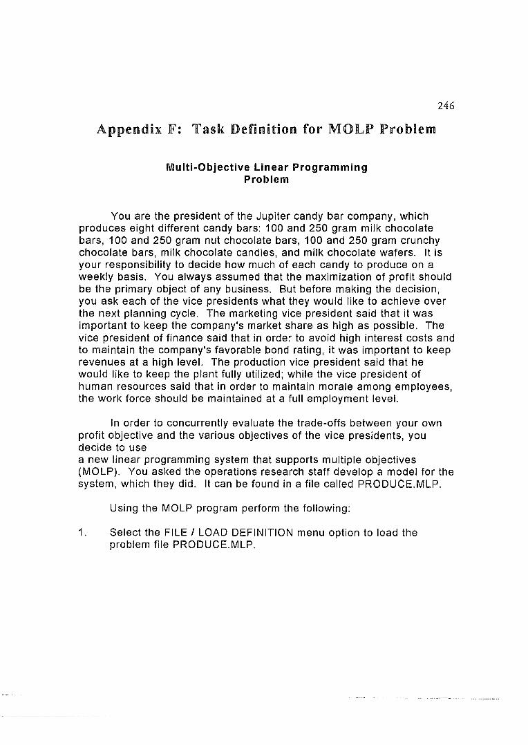
Appendix F: Tasl{ Definition for MOLP Problem
Multi-Objective Linear Programming Problem
246
You are the president of the Jupiter candy bar company, which produces eight different candy bars: 100 and 250 gram milk chocolate bars, 100 and 250 gram nut chocolate bars, 100 and 250 gram crunchy chocolate bars, milk chocolate candies, and milk chocolate wafers. It is your responsibility to decide how much of each candy to produce on a weekly basis. You always assumed that the maximization of profit should be the primary object of any business. But before making the decision, you ask each of the vice presidents what they would like to achieve over the next planning cycle. The marketing vice president said that it was important to keep the company's market share as high as possible. The vice president of finance said that in order to avoid high interest costs and to maintain the company's favorable bond rating, it was important to keep revenues at a high level. The production vice president said that he would like to keep the plant fully utilized; while the vice president of human resources said that in order to maintain morale among employees, the work force should be maintained at a full employment level.
In order to concurrently evaluate the trade-offs between your own profit objective and the various objectives of the vice presidents, you decide to use a new linear programming system that supports multiple objectives (MOLP). You asked the operations research staff develop a model for the system, which they did. It can be found in a file called PRODUCE.MLP.
Using the MOLP program perform the following:
1. Select the FILE I LOAD DEFINITION menu option to load the problem file PRODUCE.MLP.

247
2. Select the EDIT I VARIABLE PREFERENCES menu option to order the decision variables. The variables should be ordered as follows from least to most preferred:
1: Choc Candies, Choc Wafer
2: Mlk Choc 1 DO, Crunchy 1 ~O, Choc Nut 100
3: Mlk Choc 250, Crunchy 250, Choc Nut 250
3. Select the EDIT I OBJECTIVE PREFERENCES menu option to order the objectives. They should be ordered as follows from least to most preferred:
1: Employment
2: Mrkt-Share, Production, Revenue
3: Profit
4. Select the EXPLORE I NEW menu option to begin reviewing possible solutions.
5. Increase REVENUE; repeat this step one more time.
6. Increase MRKT-SHARE.
7. Make solution #2 the current solution.
8. Increase EMPLOYMENT.
9. Use the VIEW I NEW menu option to create charts and graphs for evaluting and comparing the solutions. If you would like to find other solutions besides the five already located, feel free to do so. Choose the solution you think is best. Remember, each of the solutions required a trade-off on at least one objective in order to improve on another. There is no solution that is clearly better than any of the others. As you use the various VIEW options, please complete the accompanying evaluation sheet. When you have chosen a solution, your tasl< is complete.

248
Appendix G: JEvaiuation of MOLP Problem
MOLP Post-test Evaluation
1. Please rate the effectiveness of each of the following views in evaluating and comparing solutions:
Poor Good Not used
Text List - Single Solution
2 3 4 5 N
Text List - Multiple Solution
2 3 4 5 N
Objective Wheel
2 3 4 5 N
Bar Graph - Single Solution
2 3 4 5 N
Bar Graph - Multiple Solution
2 3 4 5 N
Kiviat Chart
2 3 4 5 N
Line Graph
2 3 4 5 N
Color Stack
2 3 4 5 N

2. Please explain the perceived benefits of the views you found most helpful in evaluating solutions.
3. Please explain the shortcomings of the views you found least helpful in evaluating solutions.
4. Which views did you find difficult to interpret? Why?
249

250
5. Rate the usefulness and ease of use of each of the following functions:
Poor Good Not used
Variable and Objective Preference Specification
Usefulness 2 3 4 5 N Ease of Use 2 3 4 5
Item I ncreaselDecrease specification
Usefulness 2 3 4 5 N Ease of Use 2 3 4 5
View selection and specification
Usefulness 2 3 4 5 N Ease of Use 2 3 4 5
Line graph and color stack value look-up
Usefulness 2 3 4 5 N Ease of Use 2 3 4 5
View animation
Usefulness 2 3 4 5 N Ease of Use 2 3 4 5
Solution map navigation
Usefulness 2 3 4 5 N Ease of Use 2 3 4 5
6. What capabilities or functions of MOLP were not intuitive or difficult to use? How would you suggest improving any of the capabilities or functions?

251
7. What capabilities or functions of MOLP could be added that would simplify or facilitate the solution evaluation process?
8. Please rate the following:
Overall effectiveness of the MOLP software as a decision support tool in a multiobjective linear programming environment.
Poor Good
2 3 4 5
Your level of satisfaction with the solution you chose.
Poor Good
2 3 4 5
Degree to which you identified with the decision making role you were asked to assume in solving the problem. (1 = My primary interest in testing was a curiosity about the functionality of the software; 5 = I tried very hard to find what I thought was the very best possible solution.)
2 3 4 5

252
References
Aksoy, Y., "An Interactive Branch and Bound Algorithm for Bicriterion Nonconvex Mixed Integer Programming," Working Paper, Tulane University, New Orleans, Louisiana.
Aksoy, Y., "Interactive Multiple Objective Decision Making: A Bibliography (1965-1988)," Unpublished Document, Tulane University, New Orleans, Louisiana.
Alavi, M. and Henderson, J. C., "An Evolutionary Strategy For Implementing A Decision Support System," Management Science, 27(11), November 1981, pp. 1309-1323.
Alavi, M., Joachimsthaler, E. A., "Revisiting DSS Implementation Research: A Meta-Analysis of the Literature and Suggestions for Researchers," MIS Quarterly, March 1992, pp. 95-113.
Alvert, A., Massimo, A., Hans-Jakob, L., and David, A., "A Context-Oriented Approach for Decision Support," in Visualization in Human-Computer Interaction - Interdisciplinary Workshop, Springer-Verlag, Germany, 1988, pp. 137-148.
Antunes, C. H., Alvew, M. J., Silva, A. L., and Climaco, J. N., "Hidden Attributes and the Display of Information in Multiobjective Analysis," Management Science, 28(3), March 1982, pp. 236-243.
Applegate, L. M., Chen, T. T., Konsynski, B. R., and Nunamaker, J. F., "Knowledge Management in Organizational Planning," journal of Management Information Systems, 3(4), Spring 1987, pp. 18-38.
Barfield, W. and Robless, R., "The Effects of Two- or Three-Dimensional Graphics on the Problem-Solving Performance of Experienced and Novice Decision Maker," Behavior and Information Technology, 8(5), September -October 1989, pp. 369-385.
Barnsley, M. F. and Sloan, A. D., "A Better Way to Compress Images," BYTE Magazine, 13(1), January 1988, pp. 215-223.

253
Beck, D. and Elkerton, J., "Development and Evaluation of Direct Manipulation List," SIGCHI Bulletin, 20(3), January 1989, pp. 72-78.
Beddow, J., "Shape Coding of Multidimensional Data on a Microcomputer Display," in Proceedings of the First IEEE Conference on Visualization, IEEE Computer Society Press, Los Alamitos, California, 1990, pp. 238-246.
Benayoun, R., de Montgolfier, J., Tergny, J., and Laritchev, 0., "Linear Programming with Mulciple Objective Functions: Step Method (STEM)," Mathematical Programming, 1 (3), December 1971, pp. 366-375.
Benbasat, I. and Dexter, A. S., "An Investigation of the Effectiveness of Color and Graphical Information Presentation Under Varying Time Constraints," MIS Quarterly, 10 (1), March 1986, pp. 59-81.
Benbasat, I., Dexter, A. S., and Todd, P., "An Experimental Program Investigating Color-Enhanced and Graphical Information Presentation: An Integration of the Findings," Communications of the ACM, 29(11), November 1986, pp 1094-1105.
Benbasat, I., Goldstein, D. K., and Mead, M., "The Case Research Strategy in Studies ofinformation Systems," MIS Quarterly, 11 (3),September 1987, pp. 369-386.
Benbasat, I., Lim, F. J., and Todd, P., "The User-Computer Interface in Systems Design," Informatica, 1 (1), December 1992, pp. 62-95.
Benson, H. P. and Aksoy, Y., "Using Efficient Feasible Directions in Interactive Multiple Objective Linear Programming," Operatio1lS Research Letters, 10(4), June 1991, pp. 203-209.
Benson, H. P., "Complete Efficiency and the Initialization of Algorithms for Multiple Objective Programming," Operations Research Letters, 10(8), November 1991, pp. 481-487.
Bertin, J., Semiology of Graphics, The University of Wisconsin Press, Madison, Wisconsin, 1983.
Boehm, B. W., "Improving Software Productivity," IEEE Computer, September 1987, pp. 43-57.

254
Brittain, D., Aller, J.,Wilson, M., Wang, S. c., "Design of an End-User Visualization System," in Proceedings of the First IEEE Conference on Visualization, IEEE Computer Society Press, Los Alamitos, California, 1990, pp. 323-328.
Brown, J. R. and Cunningham, S., "Visualization in Higher Education," Academic Computing, 4(6), March 1990, pp. 24-26, 41-45.
Brown, L., "Graphical User Interfaces - A Developer's Quandary," Patricia Seybold's UNIX in the Office, 4(8), August 1989, pp. 1-12.
Campbell, H. G., An Introduction to Matrices, Vectors, and Linear Programming, Meridith Publishing Co., New York, 1965.
Campbell-Grant, I. R. and Robinson, P. J., "An Introduction to ISO DIS 8613, 'Office Document Architecture,' and Its Application To Computer Graphics," Computers & Graphics, 11 (4), 1987, pp. 325-341.
Caplinger, M., "Graphical Database Browsing," ACM SIGOIS Proceedings, October 1986, pp. 113-119.
Card, S. K., Moran, T. P., and Newell, A., The Psychology of Human-Computer Interaction, Lawrence ErIbaum Associates, Hillsdale, New Jersey, 1983.
Card, S. K., Mackinlay, J. D., and Robertson, G. G., "A Morphological Analysis of the Design Space of Input Devices," ACM Transactions on Information Systems, 9(2), April 1991, pp. 99-122.
Card, S. K., Robertson, G. G., and Mackinlay J. D., "The Information Visualizer, An Information Workspace," in Proceeding ACM CHI'91 Human Factors in Computing Systems Conference, (New Orleans, Louisiana, April 27 - May 2) ACM, New York, 1992, pp. 181-188.
Chang, N. S. and Fu, K. S., "Picture Query Languages for Pictorial Data-Base Systems," IEEE Computer, November 1981, pp. 23-33.
Chang, S., "Visual Languages: A Tutorial and Survey," IEEE Software, January 1987, pp. 29-39.
255
Chang, S., "Visual Reasoning for Information Retrieval from Very Large Databases," journal of Visual Languages and Computing, 1 (1), March 1990, pp. 41-58.
Chankong, V. and Haimes, Y. Y., North-Holland Series in System Science and Engineering - Multiobjective Decision Making: Theory and Methodology, vol 8, Elsevier Science Publishing Co., Inc., New York, 1983.
Chen, P. and Harrison, M. A., "Multiple Representation Document Development," Unpublished paper, University of California, Berkeley, California, #UCB/CSD87/367, July 30, 1987.
Chimera, R., "Value Bars: An Information and Navigation Tool for MultiAttribute Listing," in Proceedings ACM CHI '92 Human Factors in Computing Systems Conference (San Francisco May 3-7), ACM, New York, 1992, pp. 293-294.
Cleveland, W. S. and McGill, R., "Graphical Perception: Theory Experimentation, and Application to the Development of Graphical Methods," journal of the American Statistical Association 79(387), September 1984, pp. 531-553.
Coad, P. and Yourdon, E., Object-Oriented Anallysis, Prentice Hall, Englewood Cliff, New Jersey, 1990.
Coli, R. A., CoIl, J. H. and Thakur, G., "Graphs and Tables A Four-Factor Experiment," Communications of the ACM, 37(4), April 1994, pp. 77-86.
Cooper, E. M. and Larsen, G., "Presentation Graphics Theory and Use: A Comparison of Collegiate Faculty and Industrial Graphics Users," Collegiate Microcomputer, 10(1), February 1992, pp. 15-19.
Cox, D. J., "The Art of Scientific Visualization," ACtldemic Computing, 4(6), March 1990, pp. 20-22, 32-40.
Davis, L. R., "Report Format and the Decision Maker's Task: An Experimental Investigation," Accounting Organizations and Society, 14(5/6), 1989, pp. 495-508.
DeFanti, T. A., Brown, M. D., and McCormick, B. H., "Visualization: Expanding Scientific and Engi neering Research Opportunities," IEEE Computer, August 1989, pp. 12-23.

256
DeSanctis, G., "Computer Graphics as Decision Aids: Directions for Research," Decision Sciences, 15, 1984 pp. 463-487.
Dickson, G. W. and Nechis, M., "Key Information System Issues for the 1980's," MIS Quarterly, September 1984, pp. 135-159.
Dickson, G. W., DeSanctis, G., and McBride, D. J., "Understanding the Effectiveness of Computer Graphics for Decision Support: A Cumulative Experimental Approach," Communications of the ACM, 29(1), January 1986, pp. 40-47.
Drew, P. G., "PAC Systems," Pixel, 1(4), November/December 1990, pp. 22-23.
Dror, M. and Gass, S. I., "Interactive Scheme for a MOLP Problem Given Two Partial 0 rders: 0 ne on Variables and 0 ne on 0 bjectives," Applied lvlathematics and Computations, 24, 1987, pp. 195-209.
Dror, M., Gass, S. I., and Yellin, A., "Experiments With an Interactive Procedure for MOLP Given Weak Orders on Variables and Objectives," European journal of Operational Research, 34(1), February 1988, pp. 78-85.
Dror, M. and Gass, S. I., "A Case for Interactive Multiobjective Linear Programming (MOLP)," in Functional Analysis, Optimization, and Mathematical Economics, edited by L. J. Leifman, Oxford University Press, Oxford, New York, 1990, pp. 222-234.
Dror, M., Shoval, P., and Yellin, A., Multiobjective Linear Programming Another DSS," Decision Support Systems, 7(3). 1991, pp. 221-232.
Dror, M., Personal Interview, at University of Arizona, March 1992.
Dyer, J. S., "A Time-Sluing Computer Program for the Solution of the Multiple Criteria Problem," Management Science, 19(12), 1973, pp. 1379-1383.
Dyer, J. S .• Fishburn. P. C., Steuer, R. E .• Wallenius, J .• and Zionts. S .• "Multiple Criteria Decision Making Multiattribute Utility Theory: The Next Ten Years." Ma1Ztlgenzent Science, 38(5). May 1992. pp. 645-654.
Ecker, J. G. and Kouada, I. A., "Finding Efficient Points for Linear Multiple Objective Programs," Mtlthemtltictll Progrtmmzing, 8(3), June 1975, pp. 375-377.
257
Ecker, J. G. and Kouada, I. A., "Finding All Efficient Extreme Points for Multiple Objective Linear Programs," Mathematical Programming, 14(2), March 1978, pp. 249-261.
Ecker, J. G., Hegner, S. S., and Kouada, I.. A., "Generating All Maximal Efficient Faces for Multiple Objective Linear Programs," Journal of Optimization Theory and Applications, 31 (3), March 1980, pp. 353-381.
Eick, S. G., Steffen, J. L., and Summer, Jr., E. E., "Seesoft - A Tool for Visualizing Line Oriented Software Statistics," IEEE Transactions on Software Engineering, 18(11), November 1992, pp. 957-968.
Eihorn, H. J. and Hogarth, R. M., "Reply to Commentaries," Decision Making, edited by D. E. Bell, H. Raiffa, and A. Tversky, Cambridge University Press, Cambridge, Massachusetts, 1988, pp. 147-151.
Elison, R., "Visualization At Work," Academic Computing, 4(6), March 1990, pp. 26-28, 54-56.
Evans, J. P. and Steuer, R. E., "A Revised Simplex Method for Linear Multiple Objective Programs," Mathematical Programming, 5(1), 1973, pp. 54-72.
Feeney, W., "Gray Scale Diagrams as Business Charts," in Proceedings of the IEEE Conference on Visualization, IEEE Computer Society Press, Los Alamitos, California, 1991, pp. 140-147.
Feiner, S. and Beshers, c., "Visualizing n-Dimensional Virtual Worlds with nVision," Computer Graphics, 24(2), March 1990, pp. 37-38.
Fiksel, J. and Hayes-Roth, F., "Knowledge Systems for Planning Support," IEEE Expert, Fall 1989, pp 16-23.
Fishburn, P. C., Decision and Vrdue Theory, John Wiley, New York, 1964.
Fishburn, P. c., "Historical Background: Expected Utility," in Nonlinear Preference and Utility Theory, Johns Hopkins University Press, Baltimore, Maryland, 1988, pp. 1-20.
Forrest, J. J. H., Tomlin, J. A., "Implementing the Simplex Method for the Optimization Subroutine Library," IBM Systems Journal, 31 (1), 1992, pp. 11-25.

258
French, S., Decision Theory: An Introduction to the Mathematics of Rationality, Wiley, New York, 1986.
Friedhoff, R. M. and Benzon, W., "Visual Experiments," in Vimalization: The Second Computer Revolution, Abrams Inc., New York, 1989, pp. 132-137.
Furnas, G. W., "Generalized Fisheye Views," in Proceedings ACM SIGCHI '86 Conference on Human Factors in Computing Systems, 1986, pp. 16-23.
Furness, T., "Exploring Virtual Worlds with Tom Furness," ACM MemberNet (a supplement to Communications of the ACM), 34(7), July 1991, pp. 1 +.
Galliers, R. D. and Land, F. F., "Choosing Appropriate Information Systems Research Methodologies," Communications o/the ACM, 30(11), November 1987, pp. 900-902.
Gass, S. I. and Dror, M., "An Interactive Approach to Multiple-Objective Linear Programming Involving Key Decision Variables," Large Scale Systems, 5(2), April 1983, pp. 95-103.
Geoffron, A. M., Dyer, J. S., and Feinberg, A., "An Interactive Approach For Multi-Criterion Optimization, With an Application to the Operation of an Academic Department," Management Science, 19(4), December, part I, 1972, pp. 357-268.
George, J. F., Easton, G. K., Nunamaker, J. F., and Northcraft, G. B., "A Study of Collaborative Group Work With and Wirhout Computer-Based Support," Information Systems Research, 1 (4), December 1990, pp. 394-415.
Gibson, D. C. and Salvendy, G., "Knowledge Representarion in Human Problem Solving: I mplications for Expert System Design," Behaviour & Information Technology, 9(3), 1990, pp. 191-200.
Gimnich R., "Implementing Direct Manipulation Query Languages Using an Adequate Data Model," in Vimalization in Human-Computer Interaction -Interdisciplinary Workshop, Springer-Verlag, Germany, 1988, pp. 227-240.
Haber, R. and Wilkenson, L., "Perceptual Components of Compurer Displays," IEEE Computer Graphics & Applications, 2(3), May 1982, pp. 23-35.

259
Haber, R. B. and McNabb, D. A., "Visualization Idioms: A Conceptual Model for Scientific Visualization System," in Visttalization in Scientific Computing, edited by G. M. Nielson and B. Shriver, IEEE Computer Society Press, Los Alamitos, California, 1990, pp. 74-93.
Harris, L. R., "User Interfaces for Inference-Based Programs," AI Expert, October 1990, pp. 42-46.
Harrison, M. D., and Dix, A. J., "Modelling the Relationship Between State and Display in Interactive Systems," in Visualization in Human-Computer Interaction - Interdisciplinary Workshop, Springer-Verlag, Germany, 1988, pp. 241-249.
Hartson, H. R. and Hix, D., "Human-Computer Interface Development: Concepts and Systems for Its Management," ACM Computing Surveys, 21(1), March 1989, pp 5-92.
Hawryszkiewycz, I. T., Database Analysis and Design, second edition, Macmillan Publishing Co., New York, 1991.
Hearn, D. and Baker, P. M., Computer Graphics, Prentice-Hall, Englewood Cliffs, New Jersey, 1986.
Heath, M. T. and Etheridge, J. A., "Visualizing the Performance of Parallel Programs," IEEE Software, September 1991, pp. 29-39.
Henderson, Jr., D. A. and Card, S. K., "Rooms: The Use of Multiple Virtual Workspaces to Reduce Space Contention in a Window-Based Graphical User Interface," ACM Transactions on Graphics, 5(3), July 1986, pp. 211-243.
Hoadley, E. D., "I nvestigating the Effects of Color," Comnwnications of the ACM, 33(2), February 1990, pp. 120-125, 139.
Horney, M., "Interactive Data Visualization in Qualitative Research," Computer Gaphics, 28(1), February 1994, pp. 38-41.
Hurwicz, L., "Optimality Criteria for Decision Making Under Ignorance," Cowles Commission DisclIssion Pater No. 370, 1951.

260
Hwang, M .. I. H. and Wu, B. J. P., "The Effectiveness ofComputeer Graphics for Decision Support: A Meta-Analytical Integration of Research Findings," Data Base, 21(2&3), Fall 1990, pp. 11-19.
Inselberg, A. and Dimsdale, B., "Parallel Coordinates: A Tool for Visualizing Multi-Dimensional Geometry," in Proceedings o/the First IEEE Conference on Visualization, IEEE Computer Society Press, Los Alamitos, California, 1990, pp. 361-375.
Isermann, H., "The Enumeration of the Set of All Efficient Solutions for a Linear Multiple Objective Program," Operational Research Quarterly, 28(3, ii), 1977, pp. 711-725.
Jarke, M. and Vassiliou, Y., "A Framework for Choosing a Database Query Language," Computing Surveys, 17(3), September 1985, pp. 313-337.
Jarvenpaa, S. L. and Dickson, G. W., "Graphics and Managerial Decision Making: Research Based Guidelines," Commtl1lications of the ACM, 31 (6), June 1988, pp. 764-773.
Jarvenpaa, S. L., "The Effect of Task Demands and Graphical Format on Information Processing Strategies," Management Science, 35(3), March 1989, pp. 285-302.
Jarvenpaa, S. L. and Blake, I., "Information Technology and Corporate Strategy: A View From the Top," Information Systems Research, 1 (4), December 1990, pp. 351-375.
Javalgi, R. G. and Jain, H. K., "Integrating Multiple Criteria Decision Making Models into the Decision Support System Framework for Marketing Decisions," Naval Research Logistics, 35(6), December 1988, pp. 575-596.
Johnson, B., "TreeViz: Treemap Visualization of Hierarchically Structured Information," in Proceedings AClvl CHI '92 Human Factors in Computing Systems Conference (San Francisco, California, May 3-7) ACM, New York, 1992, pp. 369-370.
Jordon, P. W., "Claims for Direct Manipulation Interfaces Investigated," Industrial Management & Datil Systems, 93(8), 1992, pp. 3-6.

261
Kamada, T. and Kawai, S., "A General Framework for Visualizing Abstract Objects and Relations," ACM Transactions on Graphics, 10(1), January 1991, pp. 1-39.
Kasanen, E., Ostermark, R., and Zeleny, M., "Gestalt System of Holistic Graphics: New Management Support View ofMCDM," Computer Operations Research, 18(2), 1991, pp. 233-239.
Keeney, R. L. and Raiffa, J., Decisions With Multiple Objectives: Preferences and Value Tradeoffi, John Wiley and Sons, New York, 1976.
King, T., "Drawing Character Shapes with Bezier Curves," Dr. Dobb's journal, July 1990, pp. 46-50.
King, W. R., "Strategic Planning for Management Information Systems," MIS Quarterly, March 1978, pp. 27-37.
Kiviat, P. J., "Simulation, Technology, and the Decision Process," ACM Transactions on Modeling & Computer Simulation, 1 (2), April 1991, pp. 89-98.
Koh, E., "Visualizing the Stock Market Crash," IEEE Computer Graphics and Applications, 13(2), March 1993, pp. 14-17.
Kok, M., "The Interface With Decision Makers and Some Experimental Results in I nreractive Multiple Objective Programming Methods," Europeanjournal of Operational Research, 26(1), July 1986, pp. 96-107.
Korhonen, P., VIG: A Visual Interactive Approach to Goal Programming, User's Manual, NumPlan, Nummela, Finland, version 2.20-99, September 1987.
Korhonen, P., "A Visual Reference Direction Approach to Solving Discrete Multiple Criteria Problems," European journal of Operational Research, 34(2), March 1988, pp. 152-150.
Korhonen, P., WaIIenius, J., "A Pareto Race" Naval Research Logistics, 35(6), December 1988, pp. 615-623.
Korremann, J. E. and Davis, F. D., "Decisional Conflict and User Acceptance of Multicriteria Decision-Making Aids," Decision Sciences, 22(4), September/October 1991, pp. 918-926.

262
LeBlanc, J., Ward, M. 0., and Winels, N., "Exploring n-Dimensional Databases," in Proceedings o/the First IEEE Conference on Vimalization, IEEE Computer Society Press, Los Alamitos, California, 1990, pp. 230-237.
Lee, A.S., "A Scientific Methodology for MIS Case Studies," MIS Quarterly, March 1989, pp. 33-50.
Lee, J. M. and MacLachian, J., "The Effects of 3D Imagery on Managerial Data Interpretation," MIS Quarterly, September 1986, pp. 257-269.
Legge, G. E., Gu, Y., and Luebker, A .. , "Efficiency of Graphical Perception," Perception & Psychophysics, 46(4), October 1989, pp. 365-374.
Lehman, J. A., Vogel, D., and Dickson, G .. , "Business Graphics Trends," Datamation, November 1984, pp. 119-122.
Lehman, J. A., Wetering, J. V., and Vogel, D., "Mainframe and MicrocomputerBased Business Graphics: What Satisfies Users?" Information & Management, 10(3), March 1986, pp. 133-140.
Lehman, J. A., "Business Graphics: A Taxonomy for Information Systems Managers," Data Base, Fall 1986, pp. 24-31.
Lehner, P. E., "Cognitive Factors in User/Expert-System Interaction," Human Factors, 29(1), 1987, pp. 97-109.
Leonard-Barton, D., "Implementing Structured Software Methodologies: A Case of Innovation in Process Technology," Interfaces, 17(3), May/June 1987, pp.6-17.
Liang, T. P., "Critical Success Factors of Decision Support Systems: An Experimental Study," Data Base, Winter 1986, pp. 3-15.
Lieberman, E. R., "Soviet Multi-Objective Mathematical Programming Methods: An Overview," Management Science, 37(9), September 1991, pp. 1147-1165.
Loy, S. L., "The Interaction Effects Between General Thinking Skills and an I nteractive Graphics-Based DSS to Support Problem Structuring," Decision Sciences, 22(4), September/October 1991, pp. 846-868.

263
Lucas, H. C. and Nielsen, N. R., "The Impact of the Mode of Information Presentation on Learning and Performance," Management Science, 26(10), October 1980, pp. 982-993.
Lucas, H. c., "An Experimental Investigation of the Use of Computer-Based Graphics in Decision Making," Management Science, 27(7), July 1981, pp. 757-768 ..
Lusk, E. J. and Kersnick, M., "The Effecr of Cognitive Sryle and Report Format on Task Performance: The MIS Design Consequences, "Management Science, 25(8), August 1979, pp. 787-798.
Mackinlay, J., "Automating the Design of Graphical Presentarions of Relational Information," ACM Transactions on Graphics, 5(2), April 1986, pp. 110-141.
Mackinlay, J., Card, S. K. , and Robertson, G. G., "A Semantic Analysis of rhe Design Space of Input Devices," Human-Computer Interaction, 5(2/3), 1990, pp. 145-190.
Mackinlay, J. D., Robertson, G. G., and Card, S. K., "The Perspective Wall: Detail and Context Smoothly Integrated," in Proceedings ACM CHI'91 Human Factors in Computing Systems Conference, (New Orleans, Louisiana, April 27 - May 2) ACM, New York, 1992, pp. 173-179.
Malakooti, B., "An Exact Interactive Method for Exploring rhe Efficient Facets of Multiple Objective linear programming Problems with Quasi-Concave Utility Functions," IEEE Transactions on Systems, Man, and Cybernetics, 18(5), 1989, pp. 787-801.
Malone, T. W., Grant, K. R., and Turbalc, F. A., "The Information Lens: An Intelligent System for Information Sharing in Organizations," in Proceedings ACM Chi '86 Human Factors in Computing Systems Conference, (Boston. Massachusetts, April), ACM. New York,1986. pp. 1-8.
Mantei, M. M. and Cartel, R. G. G .• "A Study of an Entity-Based Database User Interface." ACM SIGCHI Bulletin. 14(2), July 1982, pp. 5-17.
Marcotte. O. and Soland. R. M .• "An Interactive Branch-and-Bound Algorithm for M ul tiple Cri teria Optimization." Management Science, 32(1), Jan uary 1986. pp. 61-75.

264
Masud, A. S. and Hwang, C. L., "Interactive Sequential Goal Programming," Journal o/the Operation Research Society, 32(5), pp.391-400.
McCormick, B. H., "Advanced Visualization Environments: Knowledge-Based Image Modeling," in Visualization In Supercomputing, edited by R. H. Mendez, Springer-Verlag, New York, 1990, pp. 135-150.
McDonald, J. A., Stuetzle, W. and Buja, A., "Painting Multiple Views of Complex Objects," SIGPLAN Notices, 25(10), October 1990, pp. 245-257.
McNurlin, B., editor, "Experiences With Work Group Computing," liS Analyzer, 27(7), July 1989, pp. 1-14.
Meilach, D. Z., Dynamics o/Presentation Graphics, Dow Jones-Irwin, Homewood, Illinois, 1986.
Mendez, R.H., editor, "ViSC: Definition, Domain and Recommendations," in Visualization In Supercomputing, Springer-Verlag, New York, 1990, pp. 3-7.
Michalowski, W. and Szapiro, T., "A Bi-Reference Procedure for Interactive Multiple Criteria Programming," Operations Research, 40(2), March/April 1992, pp. 247-258.
H. Mihalisin, T., Timlin, J., and Schwegler, J., "Visualization and Analysis of Multi-Variate Data: A Technique for all Fields," in Proceedings o/the IEEE Conference on Visualization, IEEE Computer Society Press, Los Alamitos, California, 1991, pp. 171-178.
Morris, M. F., "Kiviat Graphs - Conventions and 'Figures of Merit,'" Pelformance Evaluation Review, 3(3), October 1974, pp. 2-9.
Musselman, K and Talavage, J., "A Tradeoff Cut Approach to Multiple Objective Optimization," Operations Research, 28(6), November/December 1980, pp. 1424-1435.
Myers, B. A., "Demonstrational Interfaces: A Step Beyond Direct Manipulation," IEEE Computer, 25(8), August 1992, pp. 61-73.
Nielson, G. M., "Visualization in Scientific Computing," IEEE Computer, August 1989, pp 10-11.
265
Nielson, G. M., Foley, T. A., Hamann, B., and Lane, D., "Visualizing and Modeling Scattered Multivariate Data," IEEE Computer Graphics & Applications, May 1991, pp. 47-55.
Neter, J., Wasserman, W. and Kutner, M. H., Applied Linear Statistical Models (second edition), Irwin, Homewood, Illinois, 1985.
Newton, M. and Watkins, J., "The Combination of Logic and Objects for Knowledge Representation," journal of Object Oriented Programming, November/December 1988, pp. 7-9.
Nii, H. P., "Blackboard Systems: the Blackboard Model of Problem Solving and the Evolution of the Blackboard Architectures," The AI Magazine, Summer 1986, pp. 38-47.
Nunamaker, J. F, Dennis, A. R., Valacich, J. S., and Vogel, D. R., "Information Technology for Negotiating Groups: Generating Options for Mutual Gain," Management Science, 37(10), October 1991, pp. 1325-1345.
Nunamaker, J. F., Dennis, A. R., Valacich, J. S., Vogel, D. R., and George, J. F., "Electronic Meeting Systems to Support Group Work," Communications of the ACM, 34(7), July 1991, pp. 40-61.
Ostle, B., Statistics in Research, The Iowa State University Press, Ames, Iowa, 1963.
Parson, A., "Better Data, Worse Decisions?" Information Strategy: The Executive's journal, Summer 1989, pp. 20-24.
Philip. J., "Algorithms for the Vector Maximization Problem," Mathematical Progrrl11zming, 1, 1972, pp. 207-278.
Preece, J., "Some HCI Issues Concerned With Displaying Quantitative Information Graphically," in Vimalization in Human-Computer Interaction -Interdisciplinary Workshop, Springer-Verlag, Germany, 1988, pp. 209-226.
Ramesh, R., Karwan, M. H., and Zionts, S., "Preference Structure Representation Using Convex Cones in Multicriteria Integer Programming," Working Paper #646, State University of New York at Buffalo, Buffalo, New York, September 1985.

266
Ramesh, R., Zionts, S., and Karwan M. K., "A Class of Practical Interactive Branch and Bound Algorithms for Multicriteria Integer Programming," European Journal of Operational Research, 26(1), July 1986, pp. 161-172.
Ramesh, R., Karwan, M. H., Zionts, S., "Interactive Multicriteria Linear Programming: An Extension of the Method ofZiollts and Wallenius," Naval Research Logistics, 36(3), June 1989, pp. 321-335.
Remus, W., "An Empirical Investigation of the Impact of Graphical and Tabular Data Presentations on Decision Making," Management Science, 30(5), May 1984, pp. 533-542.
Rietveld, P., Multiple Objective Decision Methods and Regional Planning, NorthHolland, Amsterdam, 1980.
Roberts, F. S., Measurement Theory With Applications to Decisionmaking, Utility, and the Social Sciences, Addison Wesley, Reading, Massachusetts, 1979.
Robertson, G. G., Mackinlay, J. D., and Card, S. K., "Cone Trees: Animated 3D Visualizations of Hierarchical Information," in Proceedings ACM CHI '91 Human Factors in Computing Systems Conference, (New Orleans, Louisiana, April 27 - May 2), ACM, New York 1992, pp. 189-193.
Robertson, P. K. and O'Callaghan, J. F., "The Generation of Color Sequences for Univariate and Bivariate Mapping," IEEE Computer Graphics 6-Applications, February 1986, pp. 24-31.
Roth, S. F. and Mattis, J., "Data Characterization for Intelligent Graphics Presentation," in Proceedings ACM CHI '90 Human Factors hl Computing Systems Conference (April) ACM, New York, 1990, pp. 193-200.
Rowe, J. H., "Metafiles and Computer Graphics," Computers 6- Graphics, 10(2), 1986, pp. 103-106.
Sakamura, K., Kushiki, Y. , and ada, K., "An Overview of the BTRON/286 Specification," IEEE MICRO, June 1989, pp. 14-25.
Sarkar, M. and Brown M. H., "Graphical Fisheye Views of Graphs," in Proceedings ACM CHI '92 Human Factors in Computing Systems Conference, (San Francisco, California, May 3-7) ACM, New York, 1992, pp. 83-91.

267
Schilling, D. A., McGarity, A., and ReVelle, c., "Hidden Attributes and the Display of Information in Multiobjective Analysis," Management Science, 28(3), March 1982, pp. 236-242.
Schilling, D. A., ReVelle, c., and Cohon, J., "An Approach to the Display and Analysis of Multiobjective Problems," Socio-Economic Planning Science, 17(2),1983, pp. 57-63.
Sen, T. and Boe, W. J., "A Study on Graphical Presentation Formats and Information Processing Using Query Tracing," IEEE Transactions on Systems, Man and Cybernetics, 20(1), January/February 1990, pp. 252-257.
Shin, W. S., Ravindran, A., "Interactive Multiple Objective Optimization: Survey I - Continuous Case," Computers & Operational Research, 18(1), 1991, pp. 97-114.
Shneiderman, B., "Direct Manipulation: A Step Beyond Programming Languages," IEEE Computer, 16(8), August 1983, pp. 57-69.
Siskos, J. and Despotis, D. K., "A DSS Oriented Method for Multiobjective Linear Programming Problems," Decision Support Systems, 5( 1), February 1989, pp. 47-55.
Snedecor, G. W. and Cochran, W. G., "Curvilinear Regression," Statistical Methods, (6th edition), The Iowa State University Press, Ames Iowa, 1967, pp. 447-471.
Stash, S., "A Multiple Standards Approach," Computers & Graphics, 11 (4), 1987, pp. 479-481.
Steuer, R. E., "MOLP With Interval Criterion Weights," Mtl1lf1gement Science, 23(3), 1976 pp. 305-316.
Stewart, B. S. and White, C. c., "Multiobjective A," Journal of the Associtltionfor Computing Machinery, 38(4), October 1991, pp. 775-814.
Stonebraker, M., Anton, J., and Hanson, E., "Extending a Database System with Procedures," ACM Transactions on Database Systems, 12(3), September 1987, Pl'. 350-376.

268
Stonebraker, M., Rowe, L. A., and Hirohama, M., "The Implementation of POSTGRES," IEEE Transactions on Knowledge and Data Engineering, 2(1), March 1990, pp. 125-141.
Strayer, J. K., Linear Programming and Its Applications, Stringer-Verlag, New York, New York, 1989.
Strijbosch, L. W. G., Van Doorne, A. G. M., and Selen, W. J., "A Simplified MOLP Algorithm: the MOLP-S Procedure," Computers & Operational Research, 18(8), 1991, pp. 709-716.
Sultan, A., Linear Programming: An Introduction with Application, Academic Press, San Diego, California, 1993.
Tabucanon, M. T., Studies in Production and Engineering Economics Series Multiple Criteria Decision Making in Industry, vol 8, Elsevier Science Publishing Co., New York, 1988.
Teghem, Jr., J., Dufrane, D., Thauvoye, M., and Kunsch, P., "STRANGE: An Interactive Method for Multi-Objective Linear Programming Under Uncertainty," European journal o/Operational Research, 26(1), July 1986, pp. 65-82.
Terdeman, S., editor, "Languages: Formatting Text in TPW," PC Magazine, 11 (7), April 14, 1992, pp. 411-413.
Thomsen, C. T., "The Business Instrument Panel: A New Paradigm for Interacting With Financial Data," in Proceedings ACM CHI '90 Human Factors in Computing Systems Conference, (April), ACM, New York, 1990, pp. 161-165.
Tufte, E., The Vimal Display 0/ Quantitative Information, Graphics Press, Cheshire, Connecticut, 1983.
Tufte, E.R., Envisioning Information, Graphics Press, Cheshire, Connecticut, 1990.
Tukey, P., Maloney, L., Pani, J., and Smith, S., "Human Perception and Visualization," (panel discussion) in Proceedings o/the First IEEE Conference on Vimalization, IEEE Computer Society Press, Los Alamitos, California, 1990, pp. 401-406.

269
Venkatraman, N. and Zaheer, A., "Electronic Integration and Strategic Advantage: A Quasi-Experimental Study in the I nsurance Industry," Information Systems Research, 1(4), December 1990, pp. 377-393.
Vogel, D. R. and Wetherbe, J. c., "MIS Research: A Profile of Leading Journals and Universities," Data Base, Fall 1984, pp. 3-14.
Wald, A., Statistical Decision Functions, John Wiley, New York, 1950.
Ward, M., "Visualization Research at Worcester Polytechnic Institute," Computer Graphics, 26(3), August 1992, pp. 186-187.
Warner, J., "Visual Data Analysis in the '90s," Pixel, 1 (1), January/February, 1990, pp. 40-44.
Watson, C. J., Driver, R. W., "The Influence of Computer Graphics on the Recall of Information," MIS Quarterly, March 1983, pp. 45-53.
White, Jr., C. E. and Christy, D. P., "The Information Center Concept: A Normative Model and a Study of Six Installations," MIS Quarterly, December 1987, pp. 450-458.
White, D. J., Fundamentals of Decision Theory, North Holland, New York, 1976.
Wilde, N. and Lewis, C., "Spreadsheet-Based Interactive Graphics: From Prototype to Tool,"in Proceedings AClvf CHI '90 Human Factors in Computing Systems Conference, (April), ACM, New York, 1990, pp. 153-158.
Wilson, E. V., "An Investigation of the Relative Presentation Efficiency of Computer-Displayed Graphs," Information & Management, 26(2), February 1994, pp. 105-115.
Wilson, D. A., "Class Diagrams: A Tool for Design, Documentation, and Teaching," journal o/Object Oriented Programming, January/February 1990, pp. 38-44.
Yu, P. L .and Zeleny, M., "The Set of All Nondominated Solutions in Linear Cases and a Multicriteria Simplex Method," jounwl of Mtlthematical Analysis and Applicatiom, 49(2), February 1975, pp. 430-468.

270
Zaki, M. and Salama, R., "Linkage Versus Integration for Binding Database and Interactive Graphics Systems," Information Systems, 12(1), 1987, pp. 271-280.
Zionts, S. and Wallenius, ]., "An Interactive Programming Method for Solving the Multiple Criteria Problem," Management Science, 22(6),1976, pp. 652-663.
Zionts, S., "Method for Solving Management Problems Involving Multiple Objectives," in Multiple Criteria Decision Making Theory and Application, Proceedings Third Conference, edited by G. Fandel and T. Gal, (Hagen/Konigswinter, West Germany, August 20-24, 1979) SpringerVerlag, Berlin, 1980, pp. 540-557.