Decomposing Changes in the Distributionof Real Hourly Wages in the U.S.

Ivan Fernandez-ValFranco PeracchiFrancis VellaAico van Vuuren

The Institute for Fiscal Studies

Department of Economics,

UCL

cemmap working paper CWP61/19

Decomposing Changes in the Distribution

of Real Hourly Wages in the U.S.∗

Ivan Fernandez-Val† Franco Peracchi‡ Aico van Vuuren§

Francis Vella¶

November 11, 2019

Abstract

We analyze the sources of changes in the distribution of hourly wages in the

United States using CPS data for the survey years 1976 to 2016. We ac-

count for the selection bias from the employment decision by modeling the

distribution of annual hours of work and estimating a nonseparable model of

wages which uses a control function to account for selection. This allows the

inclusion of all individuals working positive hours and thus provides a fuller

description of the wage distribution. We decompose changes in the distribu-

tion of wages into composition, structural and selection effects. Composition

effects have increased wages at all quantiles but the patterns of change are

generally determined by the structural effects. Evidence of changes in the

selection effects only appear at the lower quantiles of the female wage distri-

bution. These various components combine to produce a substantial increase

in wage inequality.

Keywords: Wage inequality, wage decompositions, nonseparability, selection bias

JEL-codes: C14, I24, J00

∗ We are grateful to useful comments and suggestions from Stephane Bonhomme, Chinhui Juhn,Ivana Komunjer, Yona Rubinstein, Sami Stouli, and Finis Welch.† Boston University‡ Georgetown University§ Gothenburg University¶ Georgetown University

1 Introduction

The dramatic increase in earnings inequality in the United States is an intensely

studied phenomenon (see, for example, Katz and Murphy 1992, Murphy and Welch

1992, Juhn et al. 1993, Katz and Autor 1999, Lee 1999, Lemieux 2006, Autor et

al. 2008, Acemoglu and Autor 2011, Autor et al. 2016, and Murphy and Topel

2016). While this literature employs a variety of measures of earnings and inequality

and utilizes different data sets, there is general agreement that earnings inequality

has greatly increased since the early 1980s. As individual earnings reflect both

the number of hours worked and the average hourly wage rate, understanding the

determinants of each is important for uncovering the sources of earnings inequality.

This paper examines the sources of changes in the distribution of hourly real wage

rates in the United States for 1975 to 2015 while accounting for the drastic changes

in employment rates and average annual hours worked which occurred throughout

this period. To provide a fuller description of the evolution of wages we include all

individuals reporting positive annual hours rather than only those working full-time

or full-year.

Figure 1 recapitulates established empirical evidence on wage inequality by pre-

senting selected quantiles of male and female real hourly wage rates from the U.S.

Current Population Survey, or March CPS. The data are for the survey years 1976 to

2016, with information on average hourly wages for the calendar years 1975 to 2015,

and refer to individuals aged 24 to 65 years at the time of the survey, who worked

a positive number of hours the previous year, and were neither in the Armed Forces

nor self-employed.1 Consider first the median male wage rate. Despite a slight

increase between 1987 and 1990, the overall trend between 1976 and 1994 was neg-

ative, reaching a minimum of 17.6 percentage points below its initial level.2 It rises

between 1994 and 2002, but falls between 2007 and 2013. The decline between 1976

and 2016 is 13.6 percentage points. The female median wage, despite occasional

dips, increases by nearly 25 percentage points over the sample period. The male

1Section 2 provides a detailed discussion of the data employed in our analysis and our sampleselection process.

2 Throughout the paper we refer to the survey year rather than the year for which the data arecollected.

1

wage profile at the 25th percentile shows the same cyclical behavior as the median

but a greater decline, especially between 1976 and 1994, resulting in a 2016 wage

18.2 percentage points below its 1976 level. In contrast, the female wage at the

25th percentile increases by about 17 percentage points. The profiles at the 10th

percentile are similar to those of the 25th and 50th.

At higher quantiles there is a small increase in the male real wage at the 75th

percentile over the sample period. However, until the late 1990s it remained below

its 1976 level before increasing throughout the last 15 years of our sample period.

The profile at the 90th percentile resembles that of the 75th percentile, although the

periods of growth have produced larger increases. For females, there has been strong

and steady growth at the 75th and 90th percentiles since 1980 with an increasing

gap between each and the median wage.

Figure 2 reports the time series behavior of the ratio of the 90th to the 10th

percentile, a commonly used summary measure of inequality. The figure confirms

the widening wage gap for both males and females with increases over the sample

period of 55 and 38 percent respectively. Rather than immediately focusing on

these ratios, we first identify the sources of the observed wage changes. The cyclical

behavior of the profiles in Figure 1 suggests that each responds to business cycle

forces, although the strength of the response varies by quantile. The behavior of

the various profiles also suggests that workers located at different points of the wage

distribution are subject to different labor market conditions.

The previous literature has emphasized two main sources of growth in wage

inequality. One is the increase in skill premia, especially the returns to education

(see for example, Juhn et al. 1993, Katz and Autor 1999, Welch 2000, Autor et

al. 2008, Acemoglu and Autor 2011, and Murphy and Topel 2016), but also the

returns to cognitive and noncognitive skills (Heckman, Stixrud and Urzua 2006).

The manner in which the prices of individual’s characteristics contribute to wages

is known as the “structural effect”. This also reflects other factors such as declining

minimum wages in real terms, the decrease in the union premium (see, for example,

DiNardo et al. 1996, Lee 1999, and Autor et al. 2016), and the increasing use of

noncompete clauses in employment contracts (Krueger and Posner 2018). The other

2

source is the change in workers’ characteristics over the period considered. These

include the increase in educational attainment, the decrease in unionization rates,

and changes in the age structure of the workforce. The large increase in female labor

force participation may have also produced changes in the labor force composition.

The contribution to changes in the distribution of hourly wages attributable to these

observable characteristics is known as the “composition effect”.

Earlier papers (see, for example, Angrist et al. 2006, and Chernozhukov et al.

2013) estimated structural and composition effects under general conditions. How-

ever, they ignore the potential selection bias from the employment outcome (see

Heckman 1974, 1979). This “selection effect” is potentially important as the move-

ments in the employment rates and the average number of annual hours worked of

both males and females, shown in Figure 3, suggest that employment behavior has

undergone changes throughout our sample period. While this may partially reflect

long-run trends, it may also capture responses to cyclical factors. It is possible that

they are also associated with unobservable features of the workforce. Moreover, just

as the returns to observable characteristics may change over time, and be differ-

ent at different points of the wage distribution, the returns to these unobservables

may also vary. For example, Mulligan and Rubinstein (2008), hereafter MR, find

that selection by females into full-time employment played an important role in ex-

plaining the variation in inequality and that the selected sample of working females

became increasingly more productive in terms of unobservables during the last three

decades of the twentieth century. Moreover this contributed to a reduction in the

gender wage gap and an increase in wage inequality for females. Maasoumi and

Wang (2019), hereafter MW, support these findings.

MR employ a separable and parametric version of the Heckman (1979) selection

model (HSM) to evaluate the role of selection in changes in the conditional mean

wage of females. However, to evaluate the impact of selection at different points

of the wage distribution requires a nonseparable model. MW do so by employing

the procedure of Arellano and Bonhomme (2017), hereafter AB, which corrects for

sample selection in quantile regression models via a copula approach. Both MR and

MW analyze wages for the selected sample of full-time workers. This facilitates the

3

use of the HSM and AB procedures, which are based on a binary selection rule.

However, as noted above, to obtain a fuller understanding of the evolution of real

wages it is important to examine the wages of all those working and account for

their hours of work decision. Figure 4 presents the fraction of workers who work

either full-time or full-year, with full-time defined as working at least 35 hours per

week and full-year as working at least 50 weeks per year. There is a large increase

in the fraction of full-time-full-year (FTFY) females, from 49 percent in 1976 to

69 percent in 2016, while the fraction of FTFY males increases only from 76 to

82 percent. However, while the fractions working full-time are increasing, there is a

substantial number of individuals who work less than full-time.

For males, the time series patterns of the wage percentiles of FTFY workers are

similar to those of all workers. This reflects that the sample of all workers is primarily

composed of FTFY workers. However, a closer examination of Figure 5 reveals some

notable difference across non-FTFY and FTFY males. At the 90th percentile the

two groups have similar wage levels and wage trends over the whole period. However,

for the 75th percentile and below the FTFY wages are clearly higher. There is a

large difference at the median, and the wage at the 5th percentile of the FTFY

group is higher for the whole period than that for the 25th percentile for the non-

FTFY group. For females, the FTFY wage levels and trends at different quantiles are

similar to those for all female workers. This is somewhat more surprising for females

given the lower proportion of female workers who are FTFY. Given this result it

is not surprising that the female FTFY wage distribution is similar to the female

non-FTFY distribution. In fact, there are instances of specific quantiles and time

periods when the females non-FTFY wage is higher than the female FTFY wage.

Similar to males, the larger relative differences in favor of the FTFY group appear

at the lower quantiles. Note that while we illustrate these differences by contrasting

these FTFY and non-FTFY categories there may exist alternative contrasts along

the annual hours distribution which would produce larger differences.

This evidence suggests the FTFY wage movements do not provide an accurate

representation of the evolution of wages for all workers. This is particularly impor-

tant when the individuals are non-FTFY due to spells of non-employment. This

4

is likely to be the case for some of the time periods in our sample as indicated by

the patterns for males in Figure 4. Given that these workers are potentially more

vulnerable, which may be reflected in their wage, it seems inappropriate to exclude

them in an evaluation of wage inequality. It is also possible that wage differences

between these two working categories might capture selection effects in addition to

structural and composition effects. Moreover, the failure to include those who do not

work FTFY means that the selection effects in earlier studies may reflect movement

from the non-FTFY to FTFY, rather than from non-employment to FTFY.

To obtain a fuller picture of the wage distribution over a period of changing em-

ployment rates and changes in average annual hours worked, we feel it is appropriate

to include all workers and account for the selection of the hours of work decision.

Thus, a more general approach would allow for different selection effects at different

points of the hours distribution while incorporating varying structural and compo-

sitional effects. We incorporate these considerations by employing the estimation

strategy proposed by Fernandez-Val, van Vuuren, and Vella (2019), hereafter FVV,

for nonseparable models with a censored selection rule. We estimate the relationship

between the individual’s hourly wage and their characteristics while accounting for

selection resulting from the individual’s location in the annual hours distribution.

The procedure employs distribution regression methods and accounts for sample se-

lection via an appropriately constructed control function. The estimator requires a

censored variable as the basis of the selection rule and this is provided by the num-

ber of annual working hours. The novelty of our paper is to decompose changes in

the wage distribution into structural, composition and selection via a model which

features a nonseparable structure and which also allows for selection into a wider

range of annual working hours. Each of these features appear to be empirically

important.

Our empirical results confirm previous findings, restricted to FTFY workers,

regarding movements in the wage distribution. Male real wages at the median or

below have decreased despite the increases in both skill premia and educational at-

tainments. The reduction primarily reflects the large wage decreases for those with

lower levels of education. Wages at the upper quantiles have increased drastically

5

due to the increasing skill premium. These two trends combine to substantially

increase male wage inequality. Female wage growth at lower quantiles is modest

although the median wage has grown steadily. Gains at the upper quantiles are

substantial and also reflect increasing returns to schooling. These factors also have

produced a substantial increase in female wage inequality. Our results also provide

new evidence regarding the changing role of selection. These changes are especially

important at the lower end of the female wage distribution. Moreover, they tend

to decrease wage growth and increase wage inequality. Despite changes in the em-

ployment levels of males, both in participation and annual hours worked, there is no

evidence that changes in selection have affected the male wage distribution. This

result is somewhat surprising since some of the variation in male participation and

hours reflects ongoing phenomena in the macro economy.

The next section discusses the data. Section 3 describes our empirical model

and defines our decomposition exercise. This section also provides a comparison of

our decomposition approach with that associated with the HSM. Section 4 presents

the empirical results. Section 5 provides some additional discussion of the empirical

results, while Section 6 presents some extensions of the decomposition exercises.

Section 7 offers some concluding comments.

2 Data

We employ micro-level data from the Annual Social and Economic Supplement

(ASEC) of the Current Population Survey (CPS), or March CPS, for the 41 survey

years from 1976 to 2016 which report annual earnings for the previous calendar

year.3 The 1976 survey is the first for which information on weeks worked and usual

hours of work per week last year are available. To avoid issues related to retirement

and ongoing educational investment we restrict attention to those aged 24–65 years

in the survey year. This produces an overall sample of 1,794,466 males and 1,946,957

females, with an average annual sample size of 43,767 males and 47,487 females. The

annual sample sizes range from a minimum of 30,767 males and 33,924 females in

3 We downloaded the data from the IPUM-CPS website maintained by the Minnesota Popula-tion Center at the University of Minnesota (Flood et al. 2015).

6

1976 to a maximum of 55,039 males and 59,622 females in 2001.

Annual hours worked are defined as the product of weeks worked and usual

weekly hours of work last year. Most of those reporting zero hours respond that they

are not in the labor force (i.e., they report themselves as doing housework, unable to

work, at school, or retired) in the week of the March survey. We define hourly wages

as the ratio of reported annual labor earnings in the year before the survey, converted

to constant 2015 prices using the consumer price index for all urban consumers,

and annual hours worked. Hourly wages are unavailable for those not in the labor

force. For the Armed Forces, the self-employed, and unpaid family workers annual

earnings or annual hours tend to be poorly measured. Thus we exclude these groups

from our sample and focus on civilian dependent employees with positive hourly

wages and people out of the labor force last year. This restricted sample contains

1,551,796 males and 1,831,220 females (respectively 86.5 percent and 94.1 percent

of the original sample of people aged 24–65), with average annual sample sizes of

37,849 males and 44,664 females. The subsample of civilian dependent employees

with positive hourly wages contains 1,346,918 males and 1,276,125 females, with an

average annual sample size of 32,852 males and 31,125 females.

The March CPS differs from the Outgoing Rotation Groups of the CPS, or ORG

CPS, which contains information on hourly wages in the survey week for those paid

by the hour and on weekly earnings from the primary job during the survey week for

those not paid by the hour. Lemieux (2006) and Autor et al. (2008) argue that the

ORG CPS data are preferable because they provide a point-in-time wage measure

and workers paid by the hour (more than half of the U.S. workforce) may recall their

hourly wages better. However, there is no clear evidence regarding differences in the

relative reporting accuracy of hourly wages, weekly earnings and annual earnings.

In addition, many workers paid by the hour also work overtime, so their effective

hourly wage depends on the importance of overtime work and the wage differential

between straight time and overtime. Furthermore, the failure of the March CPS

to provide a point-in-time wage measure may be an advantage as it smooths out

intra-annual variations in hourly wages.

There are concerns with using earnings data from either of the CPS files. First,

7

defining hourly wages as the ratio of earnings to hours worked may induce a “division

bias” (Borjas 1980). Second, CPS earnings data are subject to measurement issues,

including top-coding of earnings (Larrimore et al. 2008), mass points at zero and

at values corresponding to the legislated minimum wage (DiNardo et al. 1996),

item non-response (Meyer et al. 2015) related to extreme earnings values, earnings

response from proxies, and earnings imputation procedures (Lillard et al. 1986, and

Bollinger et al. 2019). Our use of distribution regression methods mitigates these

first two concerns. Since there is no consensus on how to best address the others,

we retain proxy responses and imputed values.

To explain the variation in hourly wage rates and annual hours of work we employ

the following conditioning variables; the individual’s age and categorical variables for

highest educational attainment (less than high-school, high-school graduate, some

college, and college or more), race (white and non white), region of residence (North-

East, South, Central, and West), and marital status (married with spouse present,

and not married or spouse not present). We also employ household composition

variables, including the number of household members and the number of children

in the household, and indicators for the presence of children under 5 years of age

and the presence of other unrelated individuals in the household.

3 Model and objects of interest

Our objective is to decompose the changes over time in individual hourly wage rates

at various points of the wage distribution into composition, structural and selection

effects. We do this by estimating a model for the observed distribution of wages

while accounting for selection and then estimating the objects of interest which

capture these three effects.

3.1 Model

We consider a version of the HSM where the censoring rule for the selection process

incorporates the information provided in the CPS on annual hours worked, rather

8

than the binary employment/non-employment decision. The model has the form:

Y = g(X, ε), if H > 0, (1)

H = max {h∗(Z, η) , 0}, (2)

where Y is the logarithm of hourly wages, H is annual hours worked, X and Z are

vectors of observable conditioning variables, with X strictly contained in Z, g and

h∗ are unknown smooth functions, and ε and η are respectively a vector and a scalar

of potentially dependent unobservable variables with strictly increasing distribution

functions (DFs) Fε and Fη. We shall refer to max{h∗, 0} as the selection rule. We

assume that ε and η are independent of Z in the total population, and that h∗ is

strictly increasing in its second argument. Equation (2) can be considered a reduced-

form representation for annual hours worked. The model is a nonparametric and

nonseparable version of the Tobit type-3 model (see, for example, Amemiya 1984,

Vella 1993, Honore et al. 1997, Chen 1997, and Lee and Vella 2006). The most

general treatment of this model, and best suited for our objectives, is provided by

FVV.4

Due to the potential dependence between ε and η, the assumption that Z is

independent of ε in the total population does not exclude their dependence in the

selected population with H > 0. FVV show that Z is independent of ε conditional

on V = FH|Z(H |Z) and H > 0, where FH|Z(h | z) = P(H ≤ h |Z = z) denotes the

conditional DF of H given Z = z, which implies that FH|Z(H |Z) is an appropriate

control function for the selected population.5 The intuition behind this result is that

V = Fη(η) under the conditions in FVV, so V can be interpreted as an index for

the error term in the hours equation. This control function can be estimated via a

distribution regression of H on all the variables in Z.

4This model could be estimated via the AB procedure although the FVV estimator is simplerto implement in this context. However, as the AB procedure only requires a binary selection ruleit is more generally applicable than the FVV estimator.

5 This result is closely related to that of Imbens and Newey (2009), who consider estimation andidentification of a nonseparable model with a single continuous endogenous explanatory variable.Their model, however, does not include a selection mechanism.

9

3.2 Counterfactual distributions

We consider linear functionals of global objects of interest, including counterfactual

DFs, constructed by integrating local objects of interest with respect to different

joint distributions of the conditioning variables and the control function.6 Counter-

factual DFs enable the construction of wage decompositions and facilitate counter-

factual analyses similar to those in DiNardo et al. (1996), Nopo (2008), Fortin et

al. (2011), and Chernozhukov et al. (2013). We focus on functionals for the selected

population. To simplify notation, we use the superscript s to denote conditioning

on H > 0. We also denote by 1(A) the indicator function of the event A.

Our decompositions are based on the following representation of the observed

DF of Y :7

GsY (y) =

∫G(y, z, v) dF s

Z,V (z, v),

where

G(y, z, v) = E[1 {g(x, ε) ≤ y} |V = v] (3)

denotes the local distribution structural function (LDSF):8

F sZ,V (z, v) =

1{h(z, v) > 0}FZ,V (z, v)∫1{h(z, v) > 0} dFZ,V (z, v)

denotes the joint DF of Z and V in the selected population, h(z, v) = h∗(z, F−1η (v)),

and FZ,V (z, v) denotes the joint DF of Z and V in the total population.

Our counterfactual DFs are constructed by combining the DFs G and FZ,V with

the selection rule (2) for different groups, each group corresponding to a different

time period or a subpopulation defined by certain characteristics. Specifically, let Gt

denote the LDSF in group t, let FZk,Vk denote the joint DF of Z and V in group k,

and let max{hr, 0} denote the selection rule in group r. The counterfactual DF of Y

when G is as in group t, FZ,V is as in group k, and the selection rule is as in group r

6We use the term local object to refer to indicate it is conditional on a given value of V.7 We refer to FVV for details8 The LDSF gives the DF of wages if all individuals with control function equal to v had

observable characteristics equal to x.

10

is defined as:

GsY〈t,k,r〉

(y) =

∫Gt(y, x, v)1{hr(z, v) > 0} dFZk,Vk(z, v)∫

1{hr(z, v) > 0} dFZk,Vk(z, v). (4)

Since the mapping v 7→ h(z, v) is monotonic, the condition hr(z, v) > 0 in (4) is

equivalent to the condition:

v > FHr |Z(0 | z), (5)

where FHr |Z(0 | z) is the probability of working zero annual hours conditional on

Z = z in group r. Given GsY〈t,k,r〉

(y), the counterfactual quantile function (QF) of Y

when G is as in group t, FZ,V is as in group k, and the selection rule is as in group r

is defined as:

qsY〈t,k,r〉(τ) = inf{y ∈ R : GsY〈t,k,r〉

(y) ≥ τ}, 0 < τ < 1, (6)

Under these definitions, the observed DF and QF of Y for the selected population

in group t are GsY〈t,t,t〉

and qsY〈t,t,t〉 respectively. FVV show that (4) and (6) are

nonparametrically identified if Zk ⊆ Zr and (XVk ∩ZVr) ⊆ ZV t, where Zk denotes

the support of Z in group k, ZVk denotes the support of Z for the selected population

in group k, namely the set of possible combinations of observable characteristics Z

and values of the control function V for the individuals in group k working a positive

number of annual hours, etc.9

Using (6), we can decompose the difference in the observed QF of Y for the

selected population between any two groups, say group 1 and group 0, as:

qsY〈1,1,1〉 − qsY〈0,0,0〉

= [qsY〈1,1,1〉 − qsY〈1,1,0〉

]︸ ︷︷ ︸[1]

+ [qsY〈1,1,0〉 − qsY〈1,0,0〉

]︸ ︷︷ ︸[2]

+ [qsY〈1,0,0〉 − qsY〈0,0,0〉

]︸ ︷︷ ︸[3]

, (7)

where [1] is a selection effect that reflects changes in the selection rule given the

joint distribution of the conditioning variables and the control function, [2] is a

composition effect that reflects changes in the joint distribution of the conditioning

variables and the control function, and [3] is a structural effect that reflects changes

9 These conditions are weaker than requiring ZVk ⊆ ZVr and ZVk ⊆ ZVt, which guaranteesthat hr and Gt are identified for all combinations of z and v over which we integrate.

11

in the conditional distribution of the outcome given the conditioning variables and

the control function.

3.3 Comparison with the Heckman selection model

When applied to changes over time in the DF of hourly wages, the decomposition (7)

yields effects that are defined differently from those derived by MR for a parametric

version of the HSM. More precisely, the selection effect in MR excludes a compo-

nent that we attribute to the selection effect, includes another that we attribute

to the composition effect, and contains one that in nonseparable models cannot be

separately identified from the structural effect.

To illustrate this, suppose that the population model in any period t is the

following fully parametric version of the HSM:

Yt = α′tXt + εt, if Ht > 0, (8)

Ht = max{γ′tZt + ηt, 0}, (9)

where the first element of the vector Xt is the constant term, and εt and ηt are

distributed independently of Zt as bivariate normal with zero means, unit variances,

and correlation coefficient ρt.10

The counterfactual mean of Y for the selected population when the local average

structural function (LASF)11 is as in group t, FZ,V is as in group k, and the selection

rule is as in group r. Using the notation above, this has the form:

µsY〈t,k,r〉 =

∫µt(x, v)1{hr(z, v} > 0) dFZk,Vk(z, v)∫

1{hr(z, v) > 0} dFZk,Vk(z, v), (10)

where:

µt(x, v) = α′tx+ ρt Φ−1(v)

denotes the LASF in group t. The observed mean of Yt for the selected population

10We present the selection rule in this censored form in order to employ our approach althoughour discussion of the HSM which follows is based on the binary rule that only 1(Ht > 0) is observed.

11 The LASF µ(x, v) = E[g(x, ε) |V = v] gives the mean value of wage if all individuals withcontrol function equal to v had observable characteristics equal to x.

12

(after integrating over the distribution of Zt) is:

µsY〈t,t,t〉 = α′t E[Xt |Ht > 0] + ρt E[λ(γ′tZt) |Ht > 0],

where λ(·) denotes the inverse Mills ratio. We decompose the difference µsY〈1,1,1〉 −

µsY〈0,0,0〉 between two time periods, t = 0 and t = 1, into selection, composition and

structural effects.

MR define the selection effect as:

ρ1 E[λ(γ′1Z1) |H1 > 0]− ρ0 E[λ(γ′0Z0) |H0 > 0].

This effect consists of the following three elements:

ρ1

∫[λ(γ′1z)Φ1(γ

′1z)− λ(γ′0z)Φ1(γ

′0z)] dFZ1(z)+

+ ρ1

[∫λ(γ′0z)Φ1(γ

′0z) dFZ1(z)−

∫λ(γ′0z)Φ0(γ

′0z) dFZ0(z)

]+

+ (ρ1 − ρ0)′ E [λ (γ′0Z1)|H0 > 0] , (11)

where Φk(γ′rz) = Φ(γ′rz)/

∫Φ(γ′rz) dFZk

(z) is the counterfactual probability of selec-

tion in group k when the selection rule is as in group r and Φ(·) denotes the standard

normal DF. The first two elements in (11) capture the effect of changes over time

in the composition of the selected population in terms of observable characteristics.

The first element results from applying the selection rule from period 0 to period 1

holding the composition of period 1 fixed, whereas the second component results

from changing the distribution of characteristics from period 1 to period 0. The

third element captures the effect of changes over time in the composition of the

selected population in terms of unobservables through the correlation coefficient.12

In our view, the first and third elements rightfully belong to the selection effect,

whereas the second element belongs to the composition effect as it is driven by

changes over time in the distribution of Z.

We now present the selection, composition and structural effects for our decom-

12 MR make the strong assumption that the distribution of the covariates does not change overtime, i.e., FZ0 = FZ1 , so the second component drops out.

13

position and compare them with the corresponding effects in MR. Plugging this

expression for the LASF µt(x, v) into (10) gives, after some straightforward calcu-

lations:

µsY〈t,k,r〉 =

∫[α′tx+ ρtλ(γ′rz)] Φk(γ

′rz) dFZk

(z).

Thus, our selection effect is:

µsY〈1,1,1〉 − µsY〈1,1,0〉

= α′1

∫x [Φ1(γ

′1z)− Φ1(γ

′0z)] dFZ1(z)+

+ ρ1

∫[λ(γ′1z)Φ1(γ

′1z)− λ(γ′0z)Φ1(γ

′0z)] dFZ1(z). (12)

The first element on the right-hand-side of (12) is the effect on the average wage

of changes over time in the composition of the selected population in terms of ob-

servable characteristics resulting from applying the selection equation from period 0

to period 1. It is positive when the selected population contains relatively more

individuals with characteristics that are associated with higher average wages. This

element is missing in the selection effect in (11). The second element is the cor-

responding effect for the unobservable characteristics and corresponds to the first

element in (11).

Our composition effect is:

µsY〈1,1,0〉 − µsY〈1,0,0〉

= α′1

[∫xΦ1(γ

′0z) dFZ1(z)−

∫xΦ0(γ

′0z) dFZ0(z)

]+

+ ρ1

[∫λ(γ′0z)Φ1(γ

′0z) dFZ1(z)−

∫λ(γ′0z)Φ0(γ

′0z) dFZ0(z)

]. (13)

The first element on the right-hand-side of (13) is the change in the average wage

resulting directly from changes over time in the distribution of the observable char-

acteristics, while its second element is the same as the second element in (11).

Finally, our structural effect is:

µsY〈1,0,0〉 − µsY〈0,0,0〉

= (α1 − α0)′ E [X0|H0 > 0] + (ρ1 − ρ0)E [λ (γ′0Z0)|H0 > 0] . (14)

The first element on the right-hand-side of (14) reflects the impact of changes over

time in the returns to observable characteristics, while the second element captures

14

the type and degree of selection and is the same as the third element in (11). As

the expectation involving the inverse Mills ratio is positive, the contribution of this

element is positive whenever ρ1 > ρ0.

Finally, we illustrate with a simple example that the two elements of the struc-

tural effect cannot generally be identified when the model is nonseparable. Consider

a multiplicative version of the parametric HSM, which is obtained by replacing (8)

with

Yt = α′tXt εt, if Ht > 0,

and weakening the parametric assumption on the joint distribution of εt and ηt by

only requiring that ηt ∼ N(0, 1) and E[εt |Zt, Ht > 0] = ρtλ(γ′tZt). In this case αt

and ρt cannot be separately identified from the moment condition:

E[Yt |Zt, Ht > 0] = α′tXt ρtλ(γ′tZt).

While this discussion focuses on the decomposition of the mean wage, others have

also investigated the decomposition of the distribution of wages. Both AB and

MW derive selection effects at different points of the distribution. That is, they

employ the Machado and Mata (2005) method to simulate the wage distribution

that would result if everybody in the population worked based on estimates of

the model’s parameters obtained via the AB procedure. Thus in this example the

AB approach would provide selection free estimates of α for the sample for which

they are identified and then simulate wages using these estimates. Thus, similar to

MR, this approach ignores the structural and composition effects operating through

the selection effects. They interpret the difference between this distribution and

the uncorrected distribution of wages as a selection effect although some of this

difference reflects composition and structural effects. This differs from our approach

which investigates the counterfactual distribution for a more “restrictive selection

regime” than is observed but in which the selection effects are not contaminated

with components of the others. Note that the term “restrictive selection regime”

implies a setting in which the participation rate is lower.

15

4 Empirical results

4.1 Hours equation

The left panel of Figure 3 plots the employment rates of males and females, defined

as the percentage of the sample reporting positive annual hours of work. The male

employment rate fluctuates cyclically around a downward trend starting at 90.0 per-

cent, falling to a minimum of 82.1 percent in 2012, and is 83.1 percent in 2016. The

female rate increases from a low of 56.5 percent in 1976 to a high of 75.3 percent in

2001, and falls to 70.0 percent in 2016. The right panel of Figure 3 plots average

annual hours of work for wage earners. For males they vary cyclically around a

slight upward trend, increasing from 2032 hours in 1976 to 2103 hours in 2016, after

reaching a maximum of 2160 hours in 2001. For females they increase rapidly from

1515 hours in 1976 to 1792 hours in 2000, then increase slowly to 1838 hours in

2016. These patterns suggest important movements along both the intensive and

extensive margins of labor supply.

An assumption of our model is that the number of annual hours of work is

continuously distributed for values above the observed minimum number of hours

worked for each year of our sample. To explore this, Figure 6 plots the DFs of annual

hours worked by those working positive annual hours, separately by gender, for the

survey years 1976, 1996 and 2016. These years are chosen to be illustrative. Our

aim is not to illustrate how the DF of hours has changed over our period, but rather

to illustrate the presence of both point masses and a continuous component in the

distribution of annual hours of work. For example, while there is a large jump in

the DF at 2080 annual hours, corresponding to the large fraction of workers working

exactly 40 hours per week for 52 weeks, we also observe a nonzero fraction of workers

at a large number of other values of annual hours of work. This indicates that the

control function also takes on a large number of values. As we do not make any

assumptions regarding the distribution of the unobservables in the hours equation,

the large spike at 2080 hours does not constitute a violation of our assumptions.

However, we acknowledge that it produces no variation in the control function at

this particular point, for given values of Z, and we explore the implications of this

16

below.

As described in more detail in the Appendix, we estimate the control function,

defined as the conditional DF of annual hours, via a logistic distribution regression of

annual hours of work on the set of conditioning variables in Z, separately by gender

and survey year, including both workers and nonworkers. The conditioning variables

in Z include a quadratic term in age, a set of indicators for the highest educational

attainment reported, an indicator for not being married with spouse present, an

indicator for being nonwhite, a set of indicators for the region of residence, linear

terms in the number of household members and the number of children in the

household, and indicators for the presence in the household of children aged less

than 5 years and of unrelated individuals. We also include the interaction of the

quadratic age term with the educational indicators.

Except for the household size and composition variables, all the other condition-

ing variables appear in both the models for annual hours and hourly wages. Thus,

variation in household size and composition provides one source of identification,

as it induces variation in the control function for the sample of workers which is

distinct from that induced by variation in the conditioning variables also included

in the model for hourly wages. While one might argue that household size and

composition may affect hourly wage rates, we regard our exclusion restrictions as

reasonable and note that similar restrictions have been previously employed (see,

for example, MR). However, given the potentially contentious use of these exclusion

restrictions, we explore the impact of not using them below. Given the selection

rule, the assumption that annual hours of work do not affect the hourly wage rate

means that the variation in hours across individuals is the other source of identifi-

cation. As our focus is on the wage equation, we do not discuss the results for the

hours equation.

4.2 Decompositions

We now estimate gender-specific wage equations for each survey year by distribu-

tion regression over the subsample with positive hourly wages. The conditioning

variables include all those present in the equation for annual hours, with the excep-

17

tion of the household size and composition variables. In addition, we include the

control function, its square, and interactions between the other conditioning vari-

ables and the control function. Decomposing the changes in the wage distribution

as shown in (7) requires a base year. The steadily increasing female participation

rate suggests that 1976 is a reasonable choice for females, as it has the lowest level

of participation over our period. One can then plausibly assume that those with a

certain combination of x and v working in 1976 also have a positive probability of

working in any other year, as required by the identification conditions outlined in

FVV. A sensible choice for males is 2010, the bottom of the Great Recession, as it

has the lowest level of participation over our sample period. The different base years

for males and females means that we can compare trends but not wage levels across

genders. Irrespective of the base year we present the changes relative to 1976.

The decompositions at the 10th, 25th, 50th, 75th, and 90th percentiles are shown

in Figures 7–11. They capture the impact of changes in the specified components.

For example, the selection effect reflects the contribution of a change in the selec-

tion process on the wage distribution. We commence with the median (Figure 9).

During our sample period, the median wage of males decreases by 13 percent while

that of females increases by 20 percent. The structural and the total effects are very

similar for males, with the small difference due to the composition effect. There is

no evidence of any change in the selection effects. The composition effect increases

the median wage by around 2 percent and most likely reflects the increasing educa-

tional attainment of the workforce. The structural component, which appears to be

strongly procylical, produces large negative effects. While there are some upturns,

coinciding with periods of economic expansion, the structural effect is negative for

the entire period. This negative structural effect is consistent with Chernozhukov

et al. (2013) who perform a similar exercise for the period 1979 to 1988 without

correcting for sample selection.

Figure 9 reveals that the increase in the female median wage is entirely driven

by the composition effect. The structural effect is negative for the whole period, but

less substantial than that for males. The contribution of the selection component is

negative but negligible. This contrasts with MR, who find that the selection effect

18

changes from negative and large to positive and large. We do not find evidence of

such a drastic effect but, as highlighted above, our definition of the selection ef-

fect differs from that employed by MR and our approach includes the non-FTFY

workers. If their assertion that the correlation between ε and η increased over time

is correct, implying that the selected sample of females became increasingly more

productive relative to the total population, then our selection effect might under-

estimate the total change in the wage distribution due to changes in the selected

sample over time. We do not, however, find support for their conclusion that the

least productive females, in terms of unobservables, were working in the 1970s and

1980s. Our selection effect measures the difference between the observed wage dis-

tribution in any given year and the counterfactual distribution if the “least likely

to participate” females among the selected sample would not have participated. If

these females would also be the most productive, this would reduce the wage in

the “counterfactual” year and reflect a positive change in the selection effect in our

figures for the 1970s and the 1980s. We find no support for a positive change in the

selection effect.

The decompositions suggest the decline in the median male wage is due to the

prices associated with the male skill characteristics. As previous evidence highlights

the returns to higher levels of schooling have generally increased, and the male labor

force has become increasingly more educated, this suggests that the returns to those

individuals with the lowest levels of education has markedly decreased. A similar

pattern is observed for the female median wage although the less substantial negative

structural impact is offset by the composition effects.

Figures 7 and 8 report the decompositions at the 10th and 25th percentiles and

they are remarkably similar for males. They suggest that the reductions in the male

wage rate capture the prices associated with the human capital of individuals located

at these lower quantiles. There is evidence of a negative structural component of

around 25 to 30 percent at each of these quantiles in both the late 1990s and the

late 2010s. While these effects are somewhat offset by the composition effects, the

overall effect on wages is negative. There are no signs of selection effects for males.

Our results at the 10th percentile for the period 1979 to 1988 appear to differ from

19

those in Chernozhukov et al. (2013). However, that study breaks the structural

effect into separate components due to changes in the mandatory minimum wage,

unionization, and the returns to any other characteristic. Not surprisingly, changes

in the mandatory minimum wage have a large impact on the 10th percentile. Our

estimate of the structural effect combines these various components and also includes

the variation in the prices of unobservables. Our results are consistent with their

study at all other percentiles.

The evidence at the 10th and 25th percentiles for females is very different to that

for males. First, there are greater differences between the 10th and 25th percentiles.

The negative structural effects for females are more evident at the 10th percentile.

The structural effects are small at the 25th percentile and offset by the composition

effects. For both the 10th and 25th percentiles the overall wage changes become

positive in the late 1990s and generally increase over the remainder of the sample.

Figures 10 and 11 present the decompositions at the 75th and 90th percentiles.

At the 75th percentile, the male wage shows a small increase. The structural com-

ponent displays a similar pattern to that for females at the lower quantiles discussed

above. That is, initially there is a large decrease before rebounding and remain-

ing relatively flat from the early 2000s. The negative changes resulting from the

structural component are not sufficiently large to dominate the positive composi-

tion effects so the overall wage growth at the 75th percentile is positive from the

early 2000s onwards.

The changes in the female hourly wage rate at the 75th percentile highlight that

the larger movements have occurred at the upper percentiles of the wage distribu-

tion. The changes in the structural component are initially negative before turning

positive around the mid 1980s. From the beginning of the 1980s the positively

trending structural component combines with the composition effect to produce a

steadily increasing wage. However, while the decomposition at the 75th percentile

suggests that the structural components are an important contribution to inequality

at higher quantiles of the distribution, the results at the 90th percentile are even

more supportive of this perspective. For males the structural component is less

negative than at lower quantiles and this, combined with the positive composition

20

effect, produces a wage gain for the whole period. For females the structural com-

ponent is positive from the middle of the 1980s and has a larger positive effect than

the composition effect. The two effects combine to produce a remarkable 41 percent

growth in the wage.

Figures 9–11 suggest that selection effects cannot explain the observed changes

in the males’ wage distribution. At the 50th, 75th and the 90th percentiles the

selection effect is essentially zero. This is not surprising as males in this area of the

wage distribution have a strong commitment to the labor force. Moreover, there is

likely to be relatively little movement on either the extensive or intensive margin

given males’ level of commitment to full-time employment. One might suspect that

it would be more likely to uncover changes in the selection effects at the lower parts

of the wage distribution as these individuals are likely to have a weaker commitment

to full-time employment or their level of employment may be reduced via spells of

unemployment. However, the evidence does not support this.

For females, there is little evidence of changes in selection at the higher quantiles.

Females located in this part of the wage distribution are likely to have had a relatively

strong commitment to employment in 1976 and thus there were no substantial moves

in their hours distribution. Moreover, these individuals are less likely to incur periods

of unemployment. However, at the 10th and 25th percentiles the selection effects

seem economically important.13 At the 10th percentile in 2016 the selection effect

contribution is 2.2 percent, while the total wage change is between 8 and 9 percent.

Thus the female wage was lowered by 2 percent due to the increased participation

of females. This is consistent with the finding by MR of “positive selection” for

the 1990s. We also find a similar relationship for the late 1970s and 1980s. Our

results generally suggest a positive relationship between the control variable V and

wages at the bottom of the distribution. This implies that those with the highest

number of working hours, after conditioning on their observable characteristics, had

the highest wages. The trends implied by our results suggest that selection becomes

more important as we move further down the female wage distribution. This is

similar to the findings of AB which studies the evolution of female wages in the

13 The confidence intervals for these selection effects are presented in Figure 12. They indicatethat for several time periods selection effects are statistically significantly different from zero.

21

British labor market for the period 1978 to 2000.

5 Discussion

We now discuss four important issues, namely, the validity of our exclusion restric-

tions, the composition of our wage sample, the exclusion of hours from the wage

equation, and the discreteness of annual hours of work.14

We noted above that the use of household composition variables as exclusion

restrictions can be seen as controversial in this setting for both males and females.

We highlight that these are the same exclusion restrictions which are employed in

the MR and MW papers. However, to provide further insight on the impact of these

exclusion restrictions we reproduced the decompositions when we first excluded the

household variables from both the hours and wage equations and then included

them in both equations. For each of these two new specifications the model is now

identified by the variation in the number of hours worked. We do not find any

remarkable changes from either model, in comparison to the specification employed

above, with respect to the presence or magnitude of selection effects. The only

notable difference is the presence of occasionally larger negative selection effects

at the bottom decile for females for the specification which excludes the family

composition variables from both equations.

Now consider the issues related to the composition of our wage sample. As

we construct our control function using the hours of annual work variable we are

imposing, for example, that an individual who works 2 hours a week for 50 weeks

of the year is the same, in terms of unobservables, as an identical individual who

works 50 hours a week for only 2 weeks. Given the interpretation of the control

function this may be unreasonable. We check for the sensitivity of our results to

this assumption by censoring the data at various points of the hours distribution.

Our empirical work above employs wages for all those working positive hours so

we reproduce the decomposition exercises after censoring the data at the 5th, 10th,

14 The discussion that follows is based on reproducing our empirical work while incorporatingthe issue under focus. Tables or graphs with the results are not included but are available fromthe authors.

22

and 25th percentiles of the hours distribution. That is, we exclude the individuals

working lower numbers of hours from our wage sample while retaining them in the

estimation of the hours equation. We also repeat the decomposition exercise using

the full time full year selection rule employed by MR. The increased censoring has

the impact of making the wage sample more homogenous. Note, however, that as

this exercise is changing the sample size of the wage sample it is not reasonable to

compare results at the same quantiles across samples. However, with the exception

of the structural effects for females at the upper quartile the results for the structural,

composition and total effects at different quantiles are very similar for the different

censoring rules and the FTFY samples. The only notable difference is the absence

of the selection effects except for the larger samples. That is, once we censor the

bottom of the hours distribution the selection effects even disappear at the lower

quantiles for females. This is consistent with our earlier discussion that the selection

effects capture the impact of the inclusion of those with a weaker commitment to

market employment. We highlight that we find no evidence of a change in selection

effects using the FTFY sample corresponding to the MR selection rule. However,

as we discussed in detail above, this reflects the different definitions of selection

effects and the inability to disentangle components of their selection effect from the

structural effect in our setting.

In addition to employing these different censoring rules based on annual hours,

we reproduce all of our empirical analysis using weekly hours rather than annual

hours. This eliminates the variation due to differences in weeks worked and avoids

the issue discussed above of treating different types of individuals, in terms of the

unobservables, as the same. We do not find any differences for the decomposition

exercises using the corresponding control functions from the two different hours

variables. This is reassuring as it suggests we are not introducing some type of

misspecification error by incorrectly treating individuals who arrive at the same

number of annual hours by different combinations of weeks and weekly hours as the

same.

Next consider the exclusion of annual hours from the hourly wage equation.

While it is not typical to include annual hours in hourly wage equations, there may

23

be reasons to expect that the number of hours worked per year matter. Despite

an early literature (see for example Barzel, 1973) on how labor productivity may

vary with hours, and some evidence of overtime premia and part-time penalties,

there has been a general lack of attention to how hourly wages vary with hours.

Most investigations focus on full-time workers ignoring the large variation in annual

hours within this category of workers. To address this issue we re-estimate the model

including annual hours as a conditioning variable and noting that the inclusion of

the control function accounts for the endogeneity of hours in addition to the selection

issues. We explore various specifications allowing hours to enter the wage model in

a variety of ways. We then evaluated the impact of various levels of annual hours

on wages. More precisely, we evaluate the effect on hourly wages of working 500,

1000, 1500 and 2000 hours per year. For males, we found that there was a highly

variable and non monotonic relationship across years. However the relationship

fluctuated wildly and there was no clear relationship. Moreover, for many years

there was no evidence of an hours effect. This evidence supports the exclusion of

hours from the wage equation in that the variability suggests an imprecise estimate

of the hours effect. For females the evidence is not as clear. The estimated premium

from working full time appears too large to be consistent with the raw data, and

there is a large increase in hourly wages from going from 1500 annual hours to 2000

annual hours. This also appears to be inconsistent with the raw data. In addition, as

with males, the estimates display big jumps (both upwards and downwards) across

years. We conclude that these effects may reflect collinearity between the control

function and the hours variable or the impact of our exclusion restrictions. Thus we

conclude that there is no strong evidence to support the inclusion of hours in the

female wage equation. Note that it is not clear what the implications for our results

of incorrectly omitting annual hours from the wage equation would be. It is possible

that the hours effect might be inappropriately attributed to the selection effect due

to the correlation between hours and the control function. However, the absence of

selection effects suggests that if the results are affected, then it is only at the lower

quantiles unless the exclusion of hours is masking the selection effects.

Finally consider the discreteness of annual hours. Figure 6 reveals a large jump

24

in the distribution function at 2080 hours for both males and females, reflecting

the large number of individuals who report working exactly 40 hours per week for

52 weeks. This and other mass points in the distribution of annual hours imply

corresponding mass points in the distribution of the control function suggesting

that it is inconsistent with being distributed uniformly. In fact, these mass points

may reflect “rounding up” by the respondents. In this case, the underlying control

function is still uniform but the estimated control function is not. One way to

investigate this is to draw from a uniform distribution between the mass points of

the estimated control function or alternatively, adding an arbitrarily small amount

of noise to the observed hours. Both methods result in exactly the same simulated

control function. With this new control function we reproduced the empirical work.

For each of the empirical exercises the introduction of the noise had no notable

consequences.

6 Extensions

We now present some extensions of the decomposition exercises presented in Sec-

tion 4.2.

6.1 Educational premia

Our results show that the structural effects are often the main source of changes

in the distribution of wages. Since substantial empirical evidence documents the

importance of education in the increasing wage dispersion (see, for example, Autor

et al. 2008, and Murphy and Topel 2016), we try to isolate the specific role of

education treating, as customary in this literature, an individual’s education level

as exogenous. Hence, we do not attempt to distinguish between whether the returns

to education have increased or whether the returns to unobserved characteristics

positively correlated with education have increased.

We represent education by three indicators for the highest education level at-

tained, namely “high school graduate,” “some college,” and “college or more”. The

25

excluded category is “high school dropout”.15 The educational attainment of the

workforce increased dramatically over our sample period. The fraction of male work-

ers with at most a high-school degree fell from 64.1 percent in 1976 to 38.4 percent in

2016, while the fraction of those with at least a college degree rose from 20.4 percent

in 1976 to 35.2 percent in 2016. The trends for females are even more striking, as

the fraction of those with at most a high-school degree fell from 69.1 percent in 1976

to 29.7 percent in 2016, while the fraction of those with at least a college degree

rose from 16.1 percent in 1976 to 40.1 percent in 2016.

We estimate the average treatment effect (ATE) of education under the as-

sumption that the data available in each survey year represent a sample of size

n, {(Hi, Yi, Zi)}ni=1, from the distribution of the random vector (H,Y, Z), where Yi

is only observed when Hi > 0 and Zi contains all the variables in Xi.16 Under

this assumption, the average effect of changing the education level from e0 to e is

estimated as:

1

ne

n∑i=1

1{Ei = e} µ(X∗i , e, Vi)−1

ne0

n∑i=1

1{Ei = e0} µ(X∗i , e0, Vi),

where Ei is education level of individual i, X∗i consists of the other conditioning

variables inXi, ne and ne0 are the number of individuals with education level equal to

e and e0 respectively, and Vi denotes the estimated control function for individual i.

The function µ is the estimated LASF based on a flexibly specified OLS regression of

log wages on X∗i , Ei, and Vi. As we use log wages these effects can all be interpreted

as percentage changes. To satisfy identification restrictions outlined by FVV, we

calculate the wage increase that workers with education level e0 would expect to

receive if they achieved a higher level of education e.

The patterns of the ATEs over the period 1976–2016 are similar for males and

females.17 The ATE for the “high school graduate” versus “high school dropout”

15 Since 1992, the CPS measures educational attainment by the highest year of school or degreecompleted rather than the previously employed highest year of school attendance. Although theeducational recode by the IPUM-CPS aims at maximizing comparability over time, there is adiscontinuity between 1991 and 1992 in how those with a high school degree and some college areclassified.

16 For simplicity we suppress the time subscript.17 The results are available from the authors.

26

contrast increases from about 25 percent at the beginning of the period to around

30 percent at the end, after peaking at around 35 percent in the late 1990s. The ATE

for the “some college” to “high school dropout” contrast starts at about 35 percent,

the same as the peak level for the high school premium, and reaches about 45 percent

at the end of the period after increasing to about 50 percent in the late 1990s. Even

with the small decline in the last 10 years, the overall increase over the period is

substantial. The ATE for the “college or more” to “high school dropout” contrast is

sizable and despite a small decline in the late 1970s (which is stronger for females), it

increases sharply between 1976 and 2016, from about 50 percent for males and about

70 percent for females to about 90 percent for both genders. We also examine the

variation in the these respective effects by estimating the quantile treatment effects

for each of these educational contrasts. Although we do not report the results we

refer to the major findings below.

These results confirm the findings from the existing literature, dating back to

Murphy and Welch (1992), that the education premia have increased remarkably

since the early 1980s. The slowest increase is for the high-school premium, especially

at the lower percentiles, while the fastest is for the college premium, especially at

the upper percentiles. These increases are neither uniform across the distribution of

wages, as they differ across percentiles, nor uniform over time, as they are mostly

concentrated during the 1980s and 1990s. Our results show that the high-school

premium tends to present an inverted U-shaped pattern, especially at the lower

percentiles, while the college premium tends to increase monotonically throughout

the period, though at a slower rate after the 1990s, especially at the lower percentiles.

As a consequence, during the 1980s and 1990s, both the high-school and the college

premia rise, especially at the higher percentiles, but the college premium increases

faster. After the 1990s, the college premium continues rising, though at a slower

rate, but the high school premium tends to fall, especially at the lower percentiles.

As both the levels and the trends of the education premia are remarkably similar

for males and females, this evidence suggests that the returns to education are not

the only contributing factors to the patterns of between-gender wage inequality.

While we do not attempt to isolate here the role of other conditioning variables,

27

they are included in the decomposition exercises presented in Section 4.2. These

decompositions reveal that the mechanisms driving wages differ both by gender and

location in the wage distribution. For males, the fall in wages at the median or

below largely reflects the increasing penalty associated with lower education and

other forces that negatively affect the lower skilled, as revealed by the large neg-

ative structural effects for this area of the wage distribution. With the general

trend towards rising educational attainments, the composition effects are positive

and partly offset the negative structural effects. However, the large and increasing

educational premium signals that the “penalty” associated with lower education has

increased. The negative structural effects for males are not restricted to the lower

part of the wage distribution. For females, there are wage increases at each quantile

we examined and these reflect, in part, positive and increasing composition effects.

Moreover, while the structural effects are generally negative for the whole period

at the 10th and 25th percentiles, they are typically positive at the quantiles we

examined above the median. Most notably, the structural effects for females are

not dampening wage growth to the same extent as for males and at some quantiles

these structural effects are even substantial contributors to wage growth. At the

lower parts of the female wage distribution the impact of selection is negative and

can be substantial. Selection effects become more important as we move down the

wage distribution. The patterns at the 10th and 25th percentiles are suggestive of

possible larger selection effects at lower percentiles.

Our investigation does not provide direct insight into the macro factors gener-

ating these wage profiles. Nor does it provide evidence on the role of particular

institutional factors which may influence certain segments of the workforce. How-

ever it does seem that the mechanisms affecting the wages at the bottom are very

different than those influencing the top. At the top the evidence is supportive of

an increasing skill premium. At the bottom it appears that the prevailing con-

siderations are those associated with decreasing protection of lower wage workers.

These include the decrease in the real value of the minimum wage, the reduction

in unionization and the union premium, and the increase in employer bargaining

power.

28

6.2 Wage Inequality

We now examine the issue of wage inequality, which rose dramatically as measured

by increases in the 90/10 interdecile ratio of 55 percent for males and 38 percent

for females. Although our evidence shows that changes in hourly wages at different

points in the distribution are affected differently by the relevant factors, we are

unable to directly infer the respective contribution of these factors to the changes in

inequality. The left panel of Figure 13 provides a decomposition of the changes in

the decile ratio for males. Recall that wage changes at the 10th percentile are due

to the large negative structural effects, with no evidence of selection effects and a

small positive composition effect at least up to the early 1990s. On the other hand,

the large gains at the 90th percentile reflect steadily increasing composition and

structural effects, with no signs of changes in selection effects. Thus, unsurprisingly,

the large increase in the decile ratio for males is mostly due to the structural effects.

The composition effects are much smaller but also tend to increase inequality, mainly

through their large positive contribution at the upper tail of the distribution.

For females the evidence is harder to interpret. There is an increasingly positive

composition effect at the first decile but the negative structural effect produces a

decline in wages. At the upper decile, there is a steadily increasing composition effect

and a structural effect which is generally increasing wages. The large increase in the

total effect for the majority of the sample period reflects the sum of these two positive

effects. At the lower decile, the evidence suggests that the changes in the selection

effects are negatively affecting wage growth, while there is no sign of selection at

the upper decile. The right panel of Figure 13 presents the decomposition of the

changes in the decile ratio for females. In the light of our previous remarks, it is not

surprising that these changes mostly reflect the structural effect. The composition

effect is negative but small, and largely acts through the lower part of the wage

distribution. The selection effect is positive and, in some periods, it contributes

a relatively large fraction of the total change. This result is consistent with MR

although it appears that our results primarily reflect the impact of selection on the

bottom of the female wage distribution.

Although our primary focus is not on gender inequality, we examine the trends in

29

the male/female ratio at different points of the wage distribution. Figure 14 reveals

several interesting findings. First, at all points of the wage distribution, females

appear to be catching up, with the greatest gains at the median or below. This

result should be treated with caution as it largely reflects a reduction in the male

wage, not an increase in the female wage. Second, the improvement in the relative

position of females is almost entirely due to structural effects. As our previous

evidence suggests that the sign and size of the structural effects varies both over

time and by location in the wage distribution, it is surprising that the impact on

the gender wage ratios is so clear. Third, the composition effects also have steadily

increased the relative performance of females at all quantiles, though the size of the

effect diminishes as we move up the wage distribution and is smallest at the upper

decile. Finally, the selection effects are increasing gender inequality, though they

only appear to play a role in the lower part of the wage distribution.

7 Conclusions

This paper documents the changes in female and male wages over the period 1976

to 2016. We decompose these changes into structural, composition and selection

components by estimating a nonseparable model with selection. We find that male

real wages at the median and below have decreased despite an increasing skill pre-

mium and an increase in educational attainment. The reduction is primarily due to

large decreases of the wages of the individuals with lower levels of education. Wages

at the upper quantiles of the distribution have increased drastically due to a large

and increasing skill premium and this has, combined with the decreases at the lower

quantiles, substantially increased wage inequality. Female wage growth at lower

quantiles is modest although the median wage has grown steadily. The increases at

the upper quantiles for females are substantial and reflect increasing skill premia.

These changes have resulted in a substantial increase in female wage inequality. As

our sample period is associated with large changes in the participation rates and

the hours of work of females we explore the role of changes in “selection” in wage

movements. We find that the impact of these changes in selection is to decrease the

wage growth of those at the lower quantiles with very little evidence of selection ef-

30

fects at other locations in the female wage distribution. The selection effects appear

to increase wage inequality.

31

References

Acemoglu D., and Autor D. (2011), “Skills, tasks and technology: Implica-

tions for employment and earnings.” In D. Card and O. Ashenfelter (eds.),

Handbook of Labor Economics, Vol. 4B: 1043–1171. Amsterdam: Elsevier Sci-

ence, North-Holland.

Amemiya T. (1984), “Tobit models: A survey.” Journal of Econometrics, 24:

3–61.

Angrist J., Chernozhukov V., and Fernandez-Val I. (2006), “Quantile

regression under misspecification, with an application to the U.S. wage struc-

ture.” Econometrica, 74: 539–563.

Arellano M., and Bonhomme S. (2017), “Quantile selection models with an

application to understanding changes in wage inequality.” Econometrica, 85:

1–28.

Autor D. H., Katz L. F., and Kearney M. S. (2008), “Trends in U.S. wage

inequality: Revising the revisionists.” Review of Economics and Statistics, 90:

300–323.

Autor D. H., Manning A., and Smith C. L. (2016), “The contribution of the

minimum wage to US wage inequality over three decades: A reassessment.”

American Economic Journal: Applied Economics, 8: 58–99.

Barzel Y.(1973). ”The determination of daily hours and wages.” Quarterly Jour-

nal of Economics, 87: 220–238.

Bollinger C. R., Hirsch B. T., Hokayem C. M., and Ziliak J. P. (2019),

“Trouble in the tails? What we know about earnings nonresponse thirty years

after Lillard, Smith, and Welch.” Journal of Political Economy, 2143–2185.

Borjas G. (1980), “The relationship between wages and weekly hours of work:

The role of division bias.” Journal of Human Resources, 15: 409–423.

Chen S., (1997), “Semiparametric estimation of the Type-3 Tobit model.” Journal

of Econometrics, 80: 1–34.

32

Chernozhukov, V., Fernandez-Val I., and Melly B. (2013), “Inference on

counterfactual distributions.” Econometrica, 81: 2205–2268.

Chernozhukov, V., Fernandez-Val I., Newey W. K., Stouli S., and

Vella F. (2019), “Semiparametric estimation of structural functions: meth-

ods and inference.” Working paper, University of Bristol.

DiNardo J., Fortin N. M., and Lemieux T. (1996), “Labor market institu-

tions and the distribution of wages, 1973–1992: A semiparametric approach.”

Econometrica, 64: 1001–1044.

Fernandez-Val I., van Vuuren A., and Vella F. (2019), “Nonseparable

sample selection models with censored selection rules.” Working paper.

Flood S., King M., Ruggles S., and Warren J. R. (2015), “Integrated

public use microdata series, Current Population Survey: Version 4.0 [Machine-

readable database].” University of Minnesota, mimeo.

Foresi S., and Peracchi F. (1995), “The conditional distribution of excess re-

turns: An empirical analysis.” Journal of the American Statistical Association,

90: 451–466.

Fortin N. M., Lemieux T., and Firpo S. (2011), “Decomposition methods

in economics.” In D. Card and O. Ashenfelter (eds.), Handbook of Labor Eco-

nomics, Vol. 4A: 1–102. Amsterdam: Elsevier Science, North-Holland.

Heckman J. J. (1974), “Shadow prices, market wages and labor supply.” Econo-

metrica, 42: 679–694.

Heckman J. J. (1979), “Sample selection bias as a specification error.” Econo-

metrica, 47: 153–161.

Heckman J. J., Stixrud J., and Urzua S. (2006), “The effects of cognitive and

noncognitive abilities on labor market outcomes and social behavior.” Journal

of Labor Economics, 24: 411–482.

33

Honore B., Kyriazidou E., and Udry C. (1997), “Estimation of type 3

tobit models using symmetric trimming and pairwise comparison.” Journal

of Econometrics, 76: 107–128.

Imbens G. W., and Newey W. K. (2009), “Identification and estimation of

triangular simultaneous equations models without additivity.” Econometrica,

77: 1481–1512.

Juhn C., Murphy K. M., and Pierce B. (1993), “Wage inequality and the

rise in returns to skill.” Journal of Political Economy, 101: 410–442.

Jun S. J. (2009), “Local structural quantile effects in a model with a nonseparable

control variable.” Journal of Econometrics, 151: 82–97.

Katz L. F., and Autor D. H. (1999), “Changes in the wage structure and

earnings inequality.” In O. Ashenfelter and D. Card (eds.), Handbook of Labor

Economics, Vol. 3A: 1463–1555. Amsterdam: Elsevier Science, North-Holland.

Katz L. F., and Murphy K. M. (1992), “Changes in relative wages, 1963–1987:

Supply and demand factors.” Quarterly Journal of Economics, 107: 35–78.

Krueger A., and Posner E. (2018), “A proposal for protecting low-income

workers from monopsony and corruption.” In J. Shambaugh and R. Nunn

(eds.), Revitalizing Wage Growth. Policies to Get American Workers a Raise,

139–156. Washington, DC: Brookings.

Larrimore J., Burkhauser R. V., Feng S., and Zayatz L. (2008), “Con-

sistent cell means for topcoded incomes in the Public Use March CPS (1976–

2007).” Journal of Economic and Social Measurement, 33: 89–128.

Lee D. S. (1999), “Wage inequality in the United States during the 1980s: Rising

dispersion or falling minimum wage?.” Quarterly Journal of Economics, 114:

977–1023.

Lee M. J., and Vella F. (2006), ”A semiparametric estimator for censored

selection models with endogeneity.” Journal of Econometrics, 130: 235–252.

34

Lemieux T. (2006), “Increasing residual wage inequality: Composition effects,

noisy data, or rising demand for skill?” American Economic Review, 96: 461–

498.

Lillard L., Smith J. P., and Welch F. (1986). “What do we really know

about wages? The importance of nonreporting and census imputation.” Jour-

nal of Political Economy, 94: 489–506.

Maasoumi E., and Wang, L. (2019), “The gender gap between earnings distri-

butions.” Journal of Political Economy, 127: 2438–2504.

Meyer B. D., Mok W. K. C., and Sullivan J. X. (2015), “Household surveys

in crisis.” Journal of Economic Perspectives, 29: 199–226.

Mulligan C., and Rubinstein Y. (2008), “Selection, investment, and women’s

relative wages over time.” Quarterly Journal of Economics, 123: 1061–1110.

Murphy K. M., and Topel R. H. (2016), “Human capital investment, inequal-

ity, and economic growth.” Journal of Labor Economics, 34: S99–S127.

Murphy K. M., and Welch F. (1992), “The structure of wages.” Quarterly

Journal of Economics, 57: 285–326.

Nopo, H. (2008), “Matching as a tool to decompose wage gaps.” Review of Eco-

nomics and Statistics, 90: 290-299.

Praestgaard J., and Wellner J. (1993), “Exchangeably weighted bootstraps

of the general empirical process.” Annals of Probability, 21: 2053–2086.

Vella F. (1993), “A simple estimator for models with censored endogenous re-

gressors.” International Economic Review, 34: 441–457.

Welch F. (2000), “Growth in women’s relative wages and inequality among men:

One phenomenon or two?” American Economic Review Papers & Proceedings,

90: 444–449.

35

1980 1990 2000 20100

20

40

60

Survey year

Hou

rly

wag

es

Males

1980 1990 2000 2010

Survey year

Females

P5 P10 P25 P50 P75 P90

Figure 1: Percentiles of real hourly wages

1980 1990 2000 20103

4

5

6

Survey year

P90

-P

10

Males

1980 1990 2000 2010

Survey year

Females

Figure 2: Decile ratios

36

1980 1990 2000 2010

60

70

80

90

Survey year

Employment rate

1980 1990 2000 2010

1600

1800

2000

2200

Survey year

Average annual hours

Males Females

Figure 3: Employment rates and average annual hours worked of employees

1980 1990 2000 201040

60

80

100

Survey year

Per

cent

Males

1980 1990 2000 2010

Survey year

FT FY FTFY

Figure 4: Fraction of wage earners working full-time (FT), full-year (FY), and full-time full-year (FTFY)

37

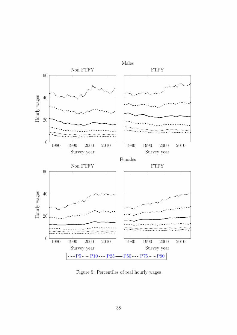
1980 1990 2000 20100

20

40

60

Survey year

Hou

rly

wag

es

Non FTFY

1980 1990 2000 2010

Survey year

FTFY

1980 1990 2000 20100

20

40

60

Survey year

Hou

rly

wag

es

Non FTFY

1980 1990 2000 2010

Survey year

FTFY

P5 P10 P25 P50 P75 P90

Males

Females

Figure 5: Percentiles of real hourly wages

38

0 1000 2000 3000 40000

0.2

0.4

0.6

0.8

1

Annual hours

Males

0 1000 2000 3000 4000

Annual hours

Females

1976 1996 2016

Figure 6: Distribution functions of positive annual hours of work

1980 1990 2000 2010

−0.4

−0.2

0

0.2

0.4

Survey year

Diff

eren

ce

Males

1980 1990 2000 2010

Survey year

Females

Selection Structural Composition Total

Figure 7: Decompositions at the 10th percentile

39

1980 1990 2000 2010

−0.4

−0.2

0

0.2

0.4

Survey year

Diff

eren

ce

Males

1980 1990 2000 2010

Survey year

Females

Selection Structural Composition Total

Figure 8: Decompositions at the 25th percentile.

1980 1990 2000 2010

−0.4

−0.2

0

0.2

0.4

Survey year

Diff

eren

ce

Males

1980 1990 2000 2010

Survey year

Females

Selection Structural Composition Total

Figure 9: Decompositions at the 50th percentile

40

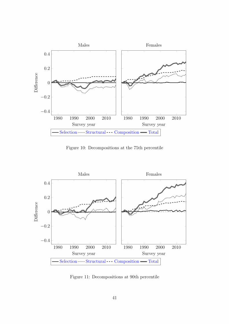
1980 1990 2000 2010

−0.4

−0.2

0

0.2

0.4

Survey year

Diff

eren

ce

Males

1980 1990 2000 2010

Survey year

Females

Selection Structural Composition Total

Figure 10: Decompositions at the 75th percentile

1980 1990 2000 2010

−0.4

−0.2

0

0.2

0.4

Survey year

Diff

eren

ce

Males

1980 1990 2000 2010

Survey year

Females

Selection Structural Composition Total

Figure 11: Decompositions at 90th percentile

41

−0.2

−0.1

0

0.1

0.2

Sel

ecti

onco

mp

onen

t

10th percentile 25th percentile

1980 1990 2000 2010−0.2

−0.1

0

0.1

0.2

Survey year

Sel

ecti

onco

mp

onen

t

50th percentile

1980 1990 2000 2010

Survey year

75th percentile

Figure 12: Selection components and associated 95% confidence intervals for femalesat various percentiles

42

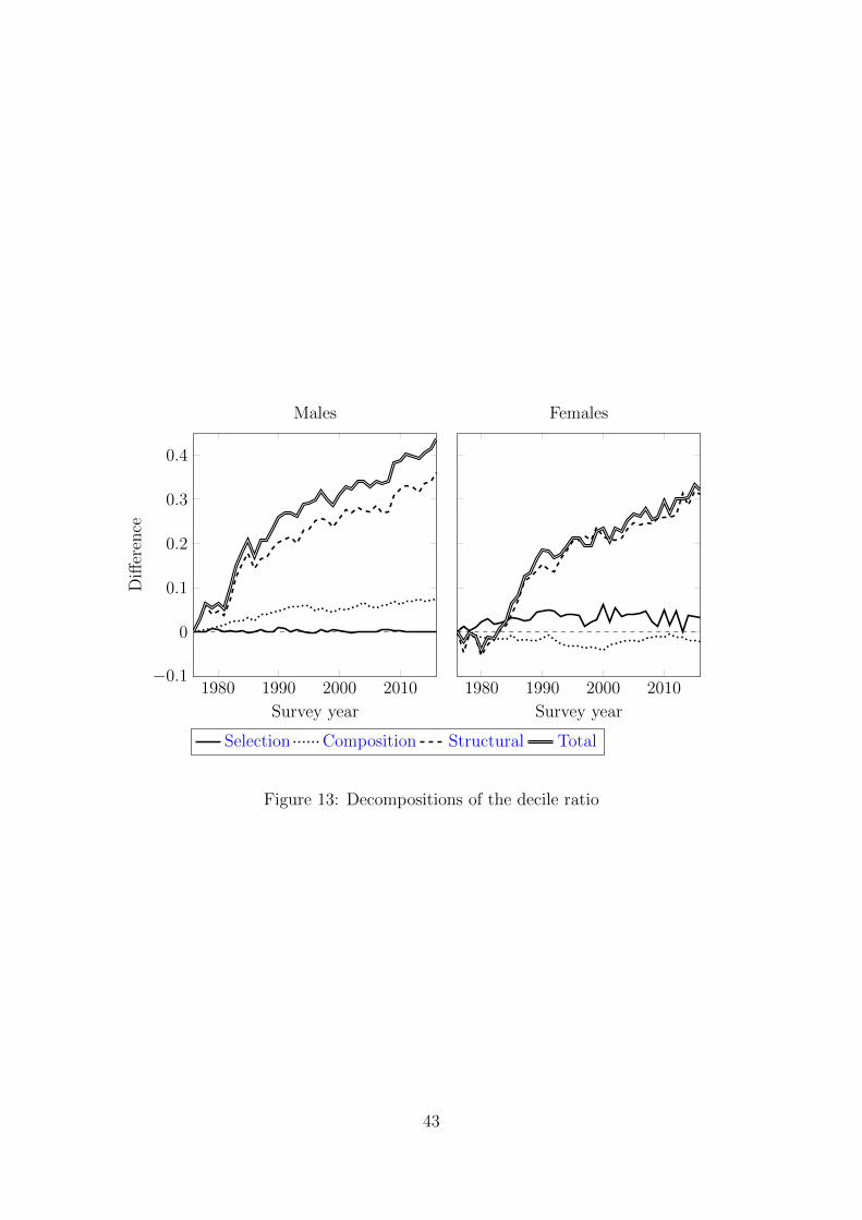
1980 1990 2000 2010−0.1

0

0.1

0.2

0.3

0.4

Survey year

Diff

eren

ce

Males

1980 1990 2000 2010

Survey year

Females

Selection Composition Structural Total

Figure 13: Decompositions of the decile ratio

43

1980 1990 2000 2010−0.4

−0.3

−0.2

−0.1

0

Diff

eren

ce10th percentile

1980 1990 2000 2010

25th percentile

1980 1990 2000 2010−0.4

−0.3

−0.2

−0.1

0

Diff

eren

ce

50th percentile

1980 1990 2000 2010

75th percentile

1980 1990 2000 2010−0.4

−0.3

−0.2

−0.1

0

Survey year

Diff

eren

ce

90th percentile

Selection Composition Structural Total

Figure 14: Decomposition of the changes in the ratio of male to female wages44

Appendix: Estimation and inference

We follow FVV and employ a multistep semiparametric method based on distribu-

tion regression to estimate the global objects of interest, namely the counterfactual

DF GsY〈t,k,r〉

(y), the counterfactual QF qsY〈t,k,r〉(τ), and the ATE of education. The

reduced-form specifications used in each step can be motivated by parametric re-

strictions on model (1)–(2). We refer to Chernozhukov et al. (2019) for examples of

such restrictions. For each group, we assume a sample of size n, {(Hi, Yi ∗ 1{Hi >

0}, Zi)}ni=1, from the distribution of the random vector (H, Y ∗1{H > 0}, Z), where

Y ∗ 1{H > 0} indicates that Y is observable only when H > 0.

In the first step we estimate the control function for each group using logistic

distribution regression (Foresi and Peracchi 1995, and Chernozhukov et al. 2013).

More precisely, for every observation in the selected sample with Hi > 0, we set:

Vi = Λ(R′iπ(Hi)), Ri = r(Zi), i = 1, . . . , n,

where Λ(u) = (1+e−u)−1 is the standard logistic DF, r(z) is a dr-dimensional vector

of transformations of z with good approximating properties (such as polynomials,

B-splines, or interactions), and:

π(h) = arg maxπ∈Rdr

n∑i=1

[1{0 < Hi ≤ h} log Λ(R′iπ)) + 1{Hi > h} log Λ(−R′iπ)] ,

for h in the empirical support Hn of H.

In the second step we estimate the LASF µ(x, v) and the LDSF G(y, x, v) for

each group using flexibly parametrized ordinary least squares (OLS) and distribu-

tion regressions, where the unknown control function is replaced by its estimator

Vi from the previous step. For reasons explained in FVV, we estimate over a sam-

ple trimmed with respect to the censoring variable H. We employ the following

trimming indicator among the selected sample:

T = 1{0 < H ≤ h}

for some h ∈ (0,∞) such that P(T = 1) > 0. The estimator of the LASF is

µ(x, v) = w(x, v)′β, where w(x, v) is a dw-dimensional vector of transformations of

45

(x, v) with good approximating properties, and β is the OLS estimator:

β =

[n∑i=1

Ti WiW′i

]−1 n∑i=1

Ti WiYi,

where Wi = w(Xi, Vi). The estimator of the LDSF is G(y, x, v) = Λ(w(x, v)′β(y)),

where y ∈ R and β(y) is the logistic distribution regression estimator:

β(y) = arg maxb∈Rdw

n∑i=1

Ti

[1{Yi ≤ y} log Λ(W ′

i b)) + 1{Yi > y} log Λ(−W ′i b))].

Finally, in the third step we use (5) to estimate the counterfactual DF (4) by:

GsY〈t,k,r〉

(y) =1

nskr

n∑i=1

Λ(W ′i βt(y))1{Vi > Λ(R′iπr(0))},

where the average is taken over the sample values of Vi and Zi in group k, nskr =∑ni=1 1{Vi > Λ(R′iπr(0))}, βt(y) is the logistic distribution regression estimator for

group t from the second step, and πr(0) is the distribution regression estimator for

group r from the first step. Given GsY〈t,k,r〉

(y), we estimate the counterfactual QF

(6) by:

qsY〈t,k,r〉(τ) = inf{y ∈ R : GsY〈t,k,r〉

(y) ≥ τ}, 0 < τ < 1.

Following FVV, inference is based on the weighted bootstrap (Praestgaard and

Wellner 1993). This method obtains the bootstrap version of the estimator of inter-

est by repeating all the estimation steps including sampling weights drawn from a

nonnegative distribution.

46