deconvolution of well test data as a nonlinear total least squares problem

8/9/2019 Deconvolution of Well Test Data as a Nonlinear Total Least Squares Problem

http://slidepdf.com/reader/full/deconvolution-of-well-test-data-as-a-nonlinear-total-least-squares-problem 1/12

SPE 71574

Deconvolution of Well Test Data as a Nonlinear Total Least Squares Problem

Thomas von Schroeter, SPE, Florian Hollaender, SPE, and Alain C. Gringarten, SPE, Imperial College, London

Copyright 2001, Society of Petroleum Engineers, Inc.

This paper was prepared for presentation at the 2001 SPE Annual Technical Con-ference and Exhibition held in New Orleans, Louisiana, 30 September – 3 October2001.

This paper was selected for presentation by an SPE Program Committee followingreview of information contained in an abstract submitted by the author(s). Contentsof the paper, as presented, have not been reviewed by the Society of PetroleumEngineers and are subject to correction by the author(s). The material, as pre-sented, does not necessarily reflect any position of the Society of Petroleum En-gineers, its officers, or members. Papers presented at SPE meetings are subjectto publication review by Editorial Committees of the Society of Petroleum Engi-neers. Electronic reproduction, distribution, or storage of any part of this paperfor commercial purposes without the written consent of the Society of PetroleumEngineers is prohibited. Permission to reproduce in print is restricted to an ab-stract of not more than 300 words; illustrations may not be copied. The abstractshould contain conspicuous acknowledgement of where and by whom the paperwas presented. Write Librarian, SPE, P.O. Box 833836, Richardson, TX 75083-3836, USA, fax 01-972-952-9435.

Abstract

Finding a good algorithm for the deconvolution of pressure

and flow rate data is one of the long-standing problems in welltest analysis. In this paper we give a survey of methods which

have been suggested in the past 40 years, and develop a new

formulation in terms of the logarithm of the response function.

The main advantage of this nonlinear encoding over prior meth-

ods is that it does not require explicit sign constraints. More-

over we introduce a new error model which accounts for errors

in both pressure and rate data; here the rates can be cumulative

or continously measured.

In this formulation, deconvolution is equivalent to a separa-

ble nonlinear Total Least Squares problem for which standard

algorithms exist. Preliminary numerical results with both sim-

ulated and field data suggest that the method is capable of pro-

ducing smooth, interpretable reservoir response estimates from

data contaminated with errors of up to 10% in rates, provided a

careful choice of weight and regularization parameters is made.

Introduction

The purpose of well test analysis is to determine geological

properties of hydrocarbon or water reservoirs from measure-

ments of wellbore pressure and production rate over time. This

involves three steps:

1. Estimating the reservoir response from the data,

2. matching the shape of the response function against a li-

brary of type curves to identify a suitable reservoir model,and

3. fitting the parameters of this model to the data.

Here the second step is mainly qualitative, while the first and

third steps are entirely quantitative.

It is solely the first step with which we shall be concerned inthis paper. As a function of time, the pressure drop is the con-

volution product of rate and reservoir response; this is the con-

tent of Duhamel’s principle. Thus, estimating the reservoir re-

sponse essentially amounts to inverting a convolution integral,

and is therefore an instance of a widely encountered mathemat-

ical problem called deconvolution.

In the simple case of a single flow period with constant rate,

the response function can be obtained (up to scale) as the deriva-

tive of the pressure drop with respect to the logarithm of time.

The standard method of obtaining response estimates is there-

fore to perform numerical differentiation on the pressure data. 4

This method has a number of serious limitations:

Numerical differentiation has the effect of amplifying

measurement errors with which the data are always con-

taminated due to limited gauge accuracy as well as exter-

nal sources of noise. The effect of gauge resolution and

the radius of investigation of a well test have been studied

in a number of publications; see Daungkaew, Hollaender

and Gringarten7 and references there.

The method extends to multirate tests, where the derivative

is formed with respect to the superposition time. 4 How-

ever, this extension is justified not so much by rigorous er-

ror analysis as by experimental evidence that it faithfully

preserves the “visual shape” of model features for a set of

standard type curves.

Moreover, even this extension cannot give response esti-

mates beyond the longest flow period with constant rate,

which reduces the radius of investigation even further.

In the narrower sense, the term deconvolution refers to the

variable rate problem only; this includes the case with multi-

ple constant flow periods. The variable rate problem has re-

ceived scant, but recurring attention over the last 40 years by

researchers both in Petroleum and Water Resources Engineer-

ing; see2,6,12 and references there. In the next section we shall

briefly sketch the main developments and summarize their mer-its and shortcomings. As for the latter ones, the two methods



2 T. VON SCHROETER, F. HOLLAENDER, A. C. GRINGARTEN SPE 71574

which were tested with simulated data seem to share a strong

sensitivity to data uncertainty once the error level reaches the

order of 5% in the pressure or 1% in the rates, which in practice

appears to be a fairly common level of uncertainty, at least as faras flow rates are concerned. Results obtained from such noisy

signals are often affected by oscillations which can render them

uninterpretable in the worst case.

In the following two sections we develop a new method which

contains two novel ideas.

The first of these is an error measure for deconvolution that

accounts for uncertainties not only in the pressure, but also

in the rate data, which are usually much less accurately mea-

sured. The resulting formulation is what is known as a Total

Least Squares (TLS) problem in the Numerical Analysis litera-

ture and as an Errors-In-Variables (EIV) problem in Statistics.

TLS has become a standard approach in many disciplines, butits application to well test analysis seems to be new.

The second idea concerns the way in which the solution

space is chosen to reflect prior knowledge about the solution.

This can be done implicitly by the way the solution space is

parametrized, or explicitly in the form of constraints on the pa-

rameters. In the Petroleum Engineering literature, the explicit

approach has a long history going back to the paper by Coats,

Rapoport, McCord, and Drews 6 who used sign constraints on

the response and its first two derivatives. Later, Kuchuk, Carter

and Ayestaran12 took up this approach in a least squares fash-

ion. Another case of was considered by Baygun, Kuchuk and

Arikan2 who used constraints on the autocorrelation sequenceand the energy of the solution vector in order to keep the solu-

tion smooth and reduce oscillations.

Our approach uses the implicit alternative instead. Its main

idea is to encode the response function in a more natural way

such that sign constraints are not necessary. This has the unwel-

come consequence of rendering the problem nonlinear; how-

ever some of this complication is offset by the reduction in the

number of constraints. In fact, our algorithm uses no constraints

at all, but just a single regularizing function which is chosen as

the “energy” of the solution, i.e. the sum of squares of its deriva-

tives on the interpolation intervals.

We explain our method in considerable detail and report pre-

liminary numerical experiments with both simulated and field

data. These experiments suggest that the method is capable

of producing smooth, interpretable reservoir response estimates

from data contaminated with fairly large errors. However, so

far practical experience is still limited, and more comprehen-

sive tests are needed. Further work is in progress.

Deconvolution and well test analysis

The foundation of well test analysis is Duhamel’s principle,

which states that the pressure drop at the wellbore is the

convolution of the flow rate and the reservoir impulse re-

sponse

as functions of time:

. . . . . . . . . . . . . . . . . . . . . . . . . . . . ( 1 )

which is shorthand for

. . . . . . . . . ( 2 )

Here and throughout the paper,

denotes the average initial

reservoir pressure and

the test duration. Flow rate and re-

sponse are assumed zero for times

. Since the introduction

of pressure derivative analysis,4 reservoir model identification

is usually based on plots of

over

. . . . . . . . . . . . . . . . . . . . . . . . (3)

Estimating this quantity from measurements of pressure andflow rate is a task which, at least in principle, amounts to in-

verting the convolution integral (2); hence the name “deconvo-

lution”.

In the case of a single flow period with constant rate, the

relation between the pressure drop and the reservoir response

simplifies to

. . . . . . . . . . . . . . . . . . . . . . . . . . . . . . . . (4)

Thus the standard method of obtaining response estimates is

to perform numerical differentiation on the pressure data with

respect to the logarithm of time.4 The limitations of this method

were discussed in the introduction.

Methods for the general case can be broadly classified into

two groups, time domain methods and spectral methods.

Time domain methods discretize the convolution integral (1)

using interpolation schemes for rate and response, and proceed

to solve the resulting linear system, which usually involves the

choice of an error measure and often also a set of constraints on

the search space of solutions. They can thus be characterized in

terms of the following ingredients:

Two sets of interpolating functions

and

suchthat rate and response can be written as

. . . . (5)

where

are the measured rates and

the response co-

efficients to be found by deconvolution. Substituting (5)

transforms (1) to a system of linear equations which can

be written in matrix form as

. . . . . . . . . . . . . . . . . . . . . . . . . . . . . . . . . . ( 6 )

where the vector has components

, the

matrix has coefficients

. . . . . . . . . . . . . . . . . . (7)



SPE 71574 DECONVOLUTION OF WELL TEST DATA AS A NONLINEAR TOTAL LEAST SQUARES PROBLEM 3

and

denotes the vector of response coefficients

. The

system (6) can be solved directly if the matrix

is square

and invertible; this is what early attempts suggested. In

practice, the second condition can hardly ever be met; thematrix

is often near rank deficient, and data are usually

affected by measurement errors. Both facts tend to con-

spire in such a way as to render results obtained by direct

inversion uninterpretable. There are two possible strate-

gies in this situation which are often combined: The first

is to impose constraints on the search space of response

coefficients

; the second is to choose the number of co-

efficients much smaller than the number of equations, and

to seek a solution of the resulting overdetermined system

in a least squares sense. We shall explain both alternatives

in turn.

Constraints on the search space of vectors express priorknowledge about the solution, for instance from physical

principles. The most obvious constraint in the case of well

test analysis is that the reservoir response cannot attain

negative values. Thus, assuming

for all

and

, we have to insist on

. . . . . . . . . . . . . . . . . . . . . . . . . . . . . . . . . . . . (8)

In fact the first and second derivative of the reservoir re-

sponse satisfy similar sign constraints, as was shown by

Coats et al.,6 who to our knowledge were also the first

to use constraints to determine response functions in the

Petroleum Engineering literature. More recently, Kuchuk

and collaborators2,12 have taken up this approach and ex-

perimented with various sets of constraints.

An error measure (or objective function)

, is primar-

ily a measure of the failure of a vector

to solve the un-

derlying linear system; it can also be used to enforce other

“desirable” features of a solution, like smoothness. The

solution is found by minimizing

over all vectors

in

the search space.

In our case, the most obvious quantity to minimize is of

course the difference between the two sides of (6), i.e. the

pressure match vector

. . . . . . . . . . . . . . . . . . . . . . . . . . . . . . ( 9 )

Mathematically the most convenient measure of this dif-

ference is its 2-norm

. . . . . . . . . . . . . . . . . . ( 1 0 )

The deconvolution problem can thus be restated as

. . . . . . . . . . . . . . . . . . . . . . . . . (11)

This is a linear least squares problem for which standard

solution procedures are available. A modern implementa-

tion would be based on the singular value decomposition

of the matrix ; see, for instance, Golub and van Loan, 10

5.5.

A choice which can be used to enforce a degree of smooth-

ness in the solution is the weighted sum

. . . . . . . . . . . . . . . ( 1 2 )

where is a discretized derivative operator such that

approximates the vector of derivatives of the solution be-

tween nodes, and is an adjustable weight. In this

formulation, deconvolution becomes a regularized least

squares problem. The solution of this problem will of

course depend on . Two main criteria for the selection

of this parameter have been suggested in the mathemat-

ical literature: the L curve criterion11 which can also be

used in the more general Total Least Squares setting to be

discussed in the following section, and cross validation, 9

which in practice is limited to the regularized least squares

problem. We shall come back to this issue later.

Table 1 summarizes what we see as the three main publi-

cations to date on time domain methods. We have not imple-

mented any of these methods ourselves, and our comments on

their performance are therefore based on the results shown in

these papers. Only the last two methods seem to have been

tested with simulated signals contaminated with varying levels

of noise. From these tests it appears that the two constrained

least squares methods give reasonable results for noise levels

of up to 2% in the pressure, but that the deconvolved response

can contain large oscillations if the error level increases to 5%.

Moreover, results with as little as 1% error in continuously mea-

sured rates seem to render results obtained with the linear set of constraints completely uninterpretable. 12

In practice, even higher error levels of up to 10% are known

to occur in measured rates. None of the methods seems to have

been tested with errors at this level.

Spectral methods have received comparatively less attention

so far. They are based on the convolution theorem of spectral

analysis which states that the convolution product commutes

with spectral transforms like the Laplace and Fourier trans-

forms. Applied to our deconvolution problem (1) this means

. . . . . . . . . . . . . . . . . . . (13)

where quantities with bar denote the transforms of the quantities

without bar. Thus an estimate for the transform of can be

obtained as

. . . . . . . . . . . . . . . . . . . . . . . . . . . . . . . . . . . . . . . ( 1 4 )

provided that and can be estimated from the data. Finally

could be estimated by applying the inverse transform to .

Alternatively, Bourgeois and Horne 5 who investigated the case

of the Laplace transform suggested that the model identification

step could be done in Laplace space.

Duhamel’s principle in the form of eq. (2) highlights a prob-

lem with this method in general: The convolution theorem (13)holds strictly only if , i.e. if we know that both pressure




Authors Year Error measure Constraints Solution method

Coats & al.6 1964 None (linear system) Signs of

and its first two derivatives Linear programming

Kuchuk & al.12 1990

Signs of

and its first two derivatives Least squares with linear inequality

constraints (active set algorithm)Baygun & al.2 1997

(

a discretized derivative), auto-

correlation coefficients of

Low-dimensional nonlinear least

squares with nonlinear constraints

Table 1. Selection of time domain methods published in the Petroleum Engineering literature.

drop and flow rate are zero after the end of the test. However,

in practice we can only know this for the rate; to wait until the

pressure has reached equilibrium level would not be economi-

cally sensible for most tests.

Numerical experiments we carried out ourselves show that

the estimates obtained with the incomplete pressure signal up

to the finite test duration tend to follow the Laplace trans-form of the correct response function truncated at time . This

observation could be practically relevant if there were reliable

numerical methods available to invert Laplace transforms taken

over finite intervals. However, this appears to be a notoriously

difficult problem itself, and the only algorithm we found in the

literature8 did not seem accurate enough for our purpose.

For the rest of the paper we shall be concerned with time

domain methods only.

Deconvolution as a bilinear TLS problem

It was already mentioned that rate uncertainties are an impor-

tant source of errors in the deconvolved response, and that noneof the deconvolution methods suggested to date accounts for

this type of uncertainty. However, only a minor modification of

the error model is required in order to allow for rate errors, as

we will presently show.

Notationsare as follows:

and

continue to denote measured

pressure and rate signals. The true, but unobserved signals are

and Æ

, where

andÆ

are signals representing the mea-

surement errors. These unobserved signals satisfy Duhamel’s

principle (cf. (1)):

Æ

. . . . . . . . . . . . . . . . ( 1 5 )

Interpolating the functions on the right hand side according to

. . . . . . . (16)

and evaluating the resulting relation at times

,

at

which the pressure measurements are taken, one obtains

Æ

. . . . . . . . . . . . . . . ( 1 7 )

where

denotes the rank 3 convolution tensor

. . . . . . . . . . . . . . . . . . . . . . . . . . . ( 1 8 )

We combine this set of equations with an error measure which

is a weighted sum of the squared norms of the two error se-

quences:

Æ

Æ

. . . . . . . . . . . . . . . . . . ( 1 9 )

where

is an adjustable weight. For instance, the choice

(20)

minimizes the sum of relative squared errors,

Æ

Æ

. . . . . . . . . . . . . (21)

In this setting, the deconvolution problem can be stated as

Æ

Æ

subject to (17). . . . . . . . . . . . . (22)

This formulation is an example of what is known as a Total Least Squares (TLS) problem in Numerical Analysis and as an

Errors-In-Variables (EIV) problem in Statistics. A different,

but equivalent formulation involving the true rates

is

. . . . . . . . . . . . . . . . . . . . . . . . . ( 2 3 )

where the vector

Æ

. . . . ( 2 4 )

whose 2-norm is minimized is called the TLS residue. Here

denotes the vector with components

. . . . . . . . . . . . . . . . . . . ( 2 5 )

Note that the residue is linear in each of the three unknowns

,

and

alone, but quadratic in the vector

of all

unknowns together!

This is an instance of a separable nonlinear least squares

problem. One of the standard algorithms for this class of prob-

lems is the Variable Projection algorithm (see, for instance,

Bjorck,3 9.4.1). The algorithm solves the more general prob-

Other norms may be more appropriate if the number and time spacing of

pressure and rate data is very different. We shall come back to this issue in thesection on “Practical details”.




lem

. . . . . . . ( 2 6 )

where the matrix and the vector are arbitrary differ-

entiable functions of . Unlike most standard algorithms for the

linear least squares problem, this algorithm is iterative and thus

requires an initial guess

.

We have implemented a version of this method and also a

regularized version with error measure

Æ

. . . . . . . . . . . . . . (27)

and regularization parameter , for which the residue is

given by

Æ

. . . . . . . . . . . . . . . . . . . . . . ( 2 8 )

Preliminary experiments suggest that deconvolved results still

show large oscillations when rates are contaminated by errors

of the order of 10%. Responses computed from field data con-

tained a number of coefficients with negative sign and were not

interpretable. Therefore we shall not include any numerical re-

sults from this method.

Our experience suggests that sign constraints are still neces-

sary if the Total Least Squares approach is used to deconvolve

linear response estimates, i.e. estimates of the function

it-self. An alternative strategy to treat the oscillation problem is to

encode the solution in a more natural way that makes sign con-

straints unnecessary. The obvious candidate for such an encod-

ing is the logarithm of the function

, which is the quantity

usually plotted over

in the diagnostic plot. This is the

approach we shall develop in the following section.

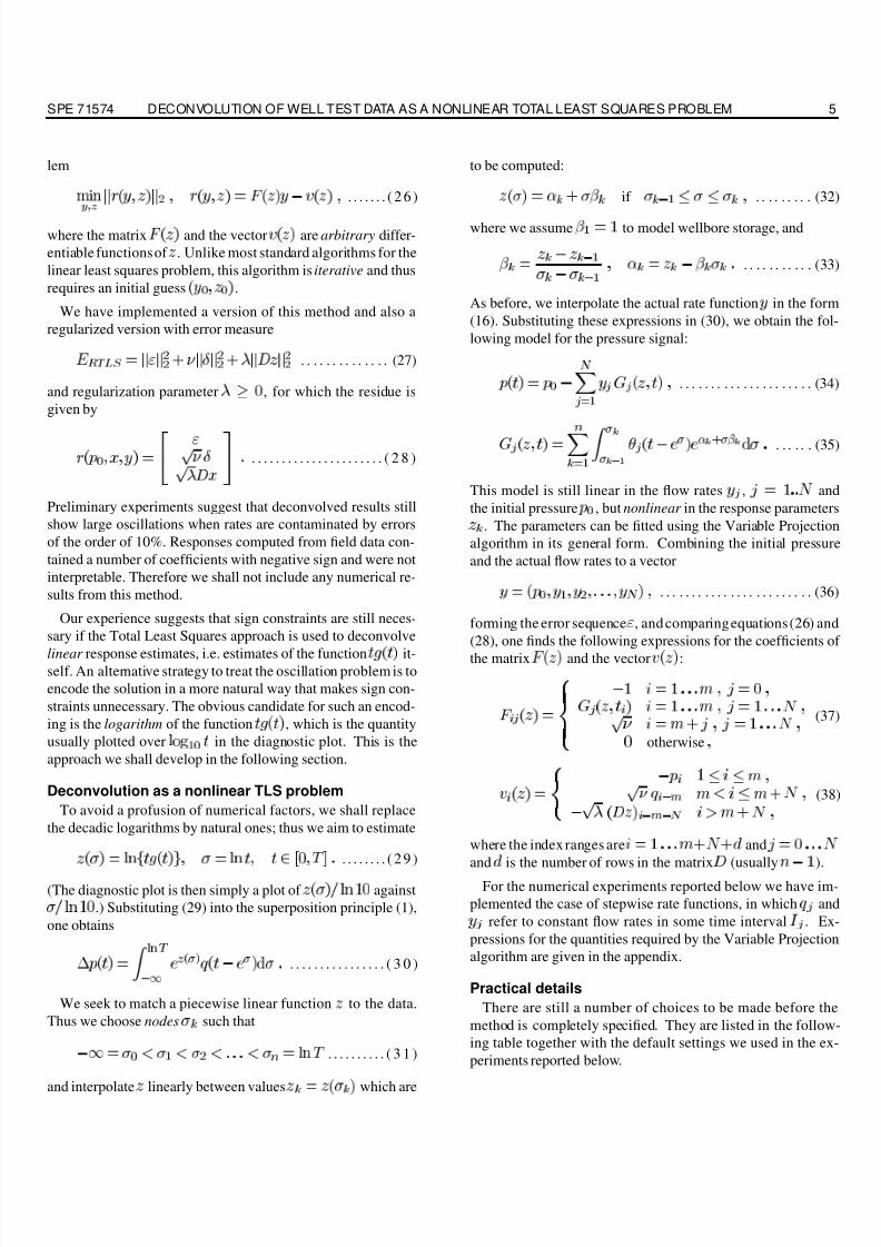
Deconvolution as a nonlinear TLS problem

To avoid a profusion of numerical factors, we shall replace

the decadic logarithms by natural ones; thus we aim to estimate

. . . . . . . . ( 2 9 )

(The diagnostic plot is then simply a plot of

against

.) Substituting (29) into the superposition principle (1),

one obtains

. . . . . . . . . . . . . . . . ( 3 0 )

We seek to match a piecewise linear function

to the data.

Thus we choose nodes

such that

. . . . . . . . . . ( 3 1 )

and interpolate

linearly between values

which are

to be computed:

if

. . . . . . . . . (32)

where we assume

to model wellbore storage, and

. . . . . . . . . . . (33)

As before, we interpolate the actual rate function in the form

(16). Substituting these expressions in (30), we obtain the fol-

lowing model for the pressure signal:

. . . . . . . . . . . . . . . . . . . . . (34)

. . . . . . (35)

This model is still linear in the flow rates

, and

the initial pressure

, but nonlinear in the response parameters

. The parameters can be fitted using the Variable Projection

algorithm in its general form. Combining the initial pressure

and the actual flow rates to a vector

. . . . . . . . . . . . . . . . . . . . . . . . (36)

forming the error sequence , and comparing equations (26) and

(28), one finds the following expressions for the coefficients of

the matrix and the vector :

otherwise

(37)

(38)

where the index ranges are

and

and

is the number of rows in the matrix

(usually

).

For the numerical experiments reported below we have im-

plemented the case of stepwise rate functions, in which

and

refer to constant flow rates in some time interval

. Ex-

pressions for the quantities required by the Variable Projection

algorithm are given in the appendix.

Practical details

There are still a number of choices to be made before the

method is completely specified. They are listed in the follow-

ing table together with the default settings we used in the ex-

periments reported below.




Parameter Default / unit Eqn.

Rate interpolation Unit rectangle (A-1)

Nodes uniform in

(41)

Regularizationmatrix

Normalizedderivative

(42)

Weight

(20)

Regularization

parameter

(47)

Starting values for

initial pressure and

rates

Starting values for

response

Wellbore storage,

then constant

(51)

Some of these choices and the way they interact require a

little more explanation:

The first node

should be chosen early enough to ensure

that the region

corresponds to wellbore storage,

which is what our model assumes. If

is chosen too late,

some of the early time features may not be visible.

If is chosen as the vector of derivatives of , then for

an arbitrary spacing of nodes we want

. . . . . . . . . . . . . . . . . . . . . . . ( 3 9 )

(not including the unit derivative for

), and thus we

need to choose

if ,

if ,

otherwise.

. . . (40)

(cf. (33)). If the nodes are uniformly spaced with step size

,

. . . . . . . . . ( 4 1 )

then

. . . . . .

. . . . . . . ( 4 2 )

Penalizing derivatives in this fashion is not the only way

to impose smoothness on the deconvolved results; another

conceivable choice is to penalize curvature instead. How-

ever so far we have not investigated this alternative.

Just as

(20) is a natural unit for the relative weight in

the error measure, there is such a unit for the regularizationparameter once a regularization matrix is chosen, as

we will now show. To ensure that the energy measure is in-

variant under subdivision of node intervals, we normalize

to unit Frobenius norm:

. . . . . . . . . . . . . . . . . . . . (43)

Then a natural, scale-invariant measure of the “relative

smoothness” of is

. . . . . . . . . . . . . . . . . . . . . . . . . . . . . . . . . . . ( 4 4 )

A dimensionless formulation of the deconvolution prob-

lem is to minimize a weighted sum of the two relative er-

rors and this smoothness measure,

Æ

. . . . . . . . . . . . . . (45)

where

and

are the dimensionless forms of their

counterparts

and

. Comparing this expression with

(see (27)), one obtains

and

. . . . . . . . . . . . (46)

with

as in (20) and

. . . . . . . . . . . . . . . . . . . . . . . . . . . . (47)

Here in practice we would suggest replacing

by the ini-

tial solution

in order to avoid updating

.

As the number of nodes is usually much smaller than the

number of pressure data points, (47) is likely to overesti-

mate the optimal regularization parameter by a factor of

roughly . It may therefore be more appropriate to

replace the discrete 2-norms by their continuous counter-

parts defined by

. . . . . . . . . . . . . . . . . . . . . . (48)

or at least to divide the 2-norms by the number of vector

components. Similar remarks apply to

if the number

and time sampling of pressure and rate data is very differ-

ent, as is likely when only an average rate is given for each

flow period.

Once the units

and

have been determined, we

choose a range of scalings around them, for instance,

. . . . . . (49)

and compute one iteration with each resulting pair .

For each value of we then plot the curves

. . . . . . . . . . . . . . . . . . . . . ( 5 0 )




parametrized by

. These are the “L curves” mentioned to

above; they are simply a visualization of the compromise

between the smoothness of

and the degree of its com-

patibility with Duhamel’s principle, given the data. Thename “L curve” refers to the shape these curve have in

regularized linear least squares problems, 11 where the the-

ory predicts a distinct point of maximal inflection which

is chosen as the optimal value of

. The observation re-

mains essentially true in our nonlinear case, even though

the curves look a little different (see Fig. 6 for an exam-

ple); thus we adopt the selection principle and pick the

pair

corresponding to the point of maximal inflec-

tion which is closest to the origin.

It remains to choose the starting point for the iteration, i.e.

the pair

.

For

there is an obvious choice, namely an estimate for

the initial pressure

obtained from the data followed by

the measured rates. As an estimate for

we simply used

the maximum of the pressure data sequence; alternatively

the first measurement could be used.

As starting point

for the response we use wellbore stor-

age (unit slope) before the first node and a constant value

afterwards,

if

if

. . . . . . . . (51)

Here continuity at the first node implies

. . . . . . . . . . . . . . . . . . . . . . . . . (52)

the value of

is determined such that the best pressure

match is obtained. In detail, evaluating (30) with the model

(51) leads to

. . . . . . . . (53)

where

. . . . . . . . . . . . . . . . . ( 5 4 )

and

. . (55)

By choosing the first node early enough, the contribution

from the early part can be made arbitrarily small.

Thus we only evaluate the remaining part at the times

of the pressure measurement, obtaining an error sequence

which in vector notation is given by

. . . . . . . . . . . . . . . . . . . . . . . . . . (56)

where the components

are computed with

the starting value of

and

denotes the matrix

......

...

(57)

The desired minimum of

is attained for

. . . . . . . . . . . . . . . . . . . . . . . . . . . . (58)

Our practical experience so far suggests that the method is

stable in the sense that results do not depend on the starting

point of the iteration. The choice we just described has

the merit of being relatively easy to compute and not too

distant from interpretable response curves, which ought to

reduce the number of iterations required for convergence.

Finally, a stopping criterion needs to be given. We stopped

the iteration when the drop in the two-norm

of the

residue fell below

of its initial value in the simulated

examples, and below

in the field examples. For both

sets of examples, this took at most 5 iterations.

Numerical results

Tests with simulated data. Figures 1–4 show results for a

simulated example; all quantities are dimensionless. The sim-

ulated reservoir behaviour is radial flow with wellbore storagecoefficient

, skin coefficient

and a sealing fault

at a distance of

wellbore radii according to the model

given by Agarwal, Al-Hussainy and Ramey. 1 Fig. 1 shows a

plot of the dimensionless pressure drop

and the derivative

as a function of

for this model (blue)

together with the corresponding curves for infinite radial flow

(black) and a linear interpolation of the simulated derivative at

nodes

. . . . . . . . . (59)

Fig. 3 shows simulated rates and pressure signals as functions

of time. The duration of the longest flow period is

,

which corresponds to the dashed line at

in Fig. 1. The

duration of the entire test is

, which corresponds to the

dashed line at

. Thus by construction the difference be-

tween the two reservoir models emerges only after the longest

rate period, and is therefore invisible for a conventional test .

Clean data are shown in black. Three levels of measurement

errors are simulated and colour-coded as follows:

Colour Pressure error Rate error

Black — —

Green 0.5 % —

Yellow 0.5 % 1 %Red 0.5 % 10 %




Here the error levels are defined as the relative variances of the

two error signals,

and Æ

. The error level

in the pressure signal would correspond to the following set of

assumptions: Permeability 100 mD, reservoir thickness 50 ft,flow rate 1000 barrels per day, viscosity 0.6 cP, pressure uncer-

tainty 2.5 psi.

The remaining process parameters were as follows:

,

, and

. Fig. 4 shows deconvolved

responses obtained with and without rate optimization. The

starting values are shown as black dots. Responses converge

rapidly towards the true derivative type curve; the maximum

number of iterations taken to reach the stopping criterion was

5. However, for 10% rate error the result with rate adaptation

is visibly smoother towards the end than the one without, even

though regularization parameters are the same. The difference

is also visible in the pressure matches for this error level (Fig.2): the match obtained with rate optimization is muchbetter. In-

creasing the regularization parameter beyond the level chosen

does not improve the deconvolved results, but tends to flatten

features and to slow down convergence. This shows that unless

rate data are very accurate, regularization alone is not always

capable of producing interpretable results and should therefore

be complemented by a more suitable error model that accounts

for rate errors.

The apparent stabilization for late times in the case with flow

rate optimization is of course a fluke and happens at the wrong

level. The remaining discrepancy at early times is probably due

to their lesser statistical weight on the linear time scale usedin the pressure match, and could be reduced by lowering the

stopping threshold.

Tests with field data. Figures 5–8 show results obtained

from the same set of field data with Bourdet’s method and with

the method suggested in this paper. The data are from the now

abandoned Maureen field and comprise 7 constant rate peri-

ods and 858 pressure data points. The entire test duration is

65 hours with no flow for the first 34 hours, which makes the

usable test duration about 31 hours. These consist of two short

and one long flow period interspersed by short buildups and fol-

lowed by a final buildup of 17 hours, which is the longest con-

stant rate period and was therefore chosen for the conventionalanalysis shown in Fig. 5. The fitted model (shown in colours)

is characterized by wellbore storage, skin, partial penetration,

radial flow and a sealing fault.

Figure 6 shows the L curves for our method obtained with the

entire data set. The optimal parameter combination (marked by

a grey dot) was found to be

(60)

Figures 7 and 8 show the first 4 iterations of deconvolved re-

sponse and pressure match for these values using 20 and 41

nodes, respectively. The nodes are spaced uniformly on the

logarithmic scale between

and 31 hours, whereas the con-

ventional method can only interpret 17 hours. Thus our method

extends the interpretable time by a factor of almost 2, corre-

sponding to one third of a log cycle.

We added a number of flow periods during the longest draw-

down to match obvious discontinuities in the pressure signal;

this is visible in the detailed pressure match in Figure 7. The

initial values for the response and the pressure data are shown

as black dots. Responses in Figures 7 and 8 are rate-normalized

whereas the conventional response shown in Figure 5 is not; this

explains the scale factor between them which is of the order of

the last rate (4100 bopd).

In both deconvolved responses, the early time features are

much less pronounced than in the conventional plot; this prob-

lem was already noted in the context of the simulated example.

Here it is probably compounded by the lack of data at earlytimes. Besides the hump due to skin seems to appear later in

the deconvolved plot.

Both deconvolved and conventional type curves show the -

1/2 slope characteristic of partial penetration, which is known

to be true. Their middle and late time behaviour is quite differ-

ent though: The deconvolved plots show a late time stabiliza-

tion at a much lower level compared with the rest of the plot.

Moreover, the plot with 41 nodes shows an intermediate level

of stabilization which does not appear in the two other plots and

could be interpreted as composite or multi-layered behaviour.

The end of the conventional response curve is badly affectedby measurement noise which is evidently amplified by numer-

ical differentiation. By construction, this source of error is not

present in our method, and thus the deconvolved responses ob-

tained with our method generally look smooth and interpretable

provided the regularization parameter is carefully chosen.

The method is currently implemented in Mathematica, a list-

based programming environment. Computation times for 41

nodes, 3 flow periods and 858 data points were about 250 sec-

onds per iteration, and thus about 1000 seconds for the four

iterations shown and for a single weight and regularization pa-

rameter. Additionally a much larger share of the total comput-

ing time is spent on finding the optimal parameter pair, even

though this part of the computation was done with only two it-

erations. Future implementations in a compiled language are

expected to run considerably faster.

Conclusions

1. The standard way in which the well test deconvolution

problem has been treated in the Petroleum Engineering lit-

erature is as a linear Least Squares problem with explicit

sign and energy constraints.

2. This strategy fails to produce interpretable results at error

levels of the order of up to 5% in the pressure signal and1% in the rate signal, as reported by the authors.




1 2 3 4 5 6log10 t0.01

0.05

0.1

0.5

1

5

10

t g(t)

Fig. 1 – Pressure and derivative type curve for radial flow

(black) and a sealing fault at 300 wellbore radii (blue) with

wellbore storage and skin coefficients CD=100 and S=5, and

interpolated derivative type curve with nodes given by eq.

(59). The two vertical lines mark the end of the longest flow

period and the end of the test.

50000 100000 150000 200000t

10

20

30

40

50

60

p(t)

Fig. 2 – Pressure matches for simulated data with 0.5% error

in the pressure and 10% in the rates. Data in black, pressure

curves with the deconvolved response in red. Dashed curve

without rate optimization, solid curve with rate optimization.

50000 100000 150000 200000t

1

2

3

4

5

q(t)

50000 100000 150000 200000t

10

20

30

40

50

60

p(t)

Fig. 3 – Rates (left) and pressure signals (right) obtained from the model response shown in Fig. 1. Clean data in black.

Simulated errors: 0.5 % in the pressure only (green); dto. with 1 % error in rates (yellow); dto. with 10 % error in the rates (red).

1 2 3 4 5 6log10 t0.01

0.05

0.1

0.5

1

5

10

t g(t)

1 2 3 4 5 6log10 t0.01

0.05

0.1

0.5

1

5

10

t g(t)

Fig. 4 – True type curve and deconvolved responses for the simulated tests shown in Fig. 3. Left: results obtained by optimizing

initial pressure and responses only. Right: results obtained by optimizing initial pressure, responses, and rates. Black dotsmark the initial response

. The two vertical lines indicate the end of the longest flow period and the end of the test.




Fig. 5 – Field example: Response estimate obtained from

final buildup only with Bourdet’s algorithm (black) togetherwith fitted reservoir model (pressure drop in red, derivative

in purple). (Output from Interpret 2000 .)

115 120 125 130 135 140ρ

0.015

0.02

0.03

0.05

0.07

ζ

Fig. 6 – L curves for the field example with 41 nodes. Weight

ranging from

(orange, hidden) to

(dark blue)and regularization parameter

ranging from

(top) to

(bottom of plot). The grey dot marks the optimal pair.

-2 -1 0 1log10t0.001

0.0015

0.002

0.003

0.005

0.007

0.01

log10tg(t)

40 42 44 46 48t (hrs)

3212.5

3215

3217.5

3220

3222.5

3225

3227.5

3230

p (psi)

Fig. 7 – Deconvolved response (in psi/bopd) and detail of the pressure match (in psi) over time (in hours) for the field example

with 20 nodes and additional flow periods. Initial response and pressure data in black. Iterations: 1st (light green), 2nd (green),

3rd (blue), 4th (purple).

-2 -1 0 1log10t0.001

0.0015

0.002

0.003

0.005

0.007

0.01

log10tg(t)

40 45 50 55 60 65t (hrs)

3220

3240

3260

3280

3300

33203340

3360p (psi)

Fig. 8 – Deconvolved response (in psi/bopd) and pressure match (in psi) over time (in hours) for the field example with 41 nodes

and additional flow periods. Initial response and pressure data in black. Iterations: 1st (light green), 2nd (green), 3rd (darkblue), 4th (red).




3. In this paper we have introduced a new method which

reformulates deconvolution as a nonlinear Total Least

Squares problem. The two main improvements are

a nonlinear encoding of the reservoir response which

makes explicit sign constraints obsolete, and

a modified error model which accounts for errors in

both pressure and rate data.

4. Preliminary experiments with simulated and field data

suggest that the new method is capable of deconvolving

smooth, interpretable response functions from data con-

taminated with errors of up to 10% in rates provided that

error weight and regularization parameter are suitably cho-

sen.

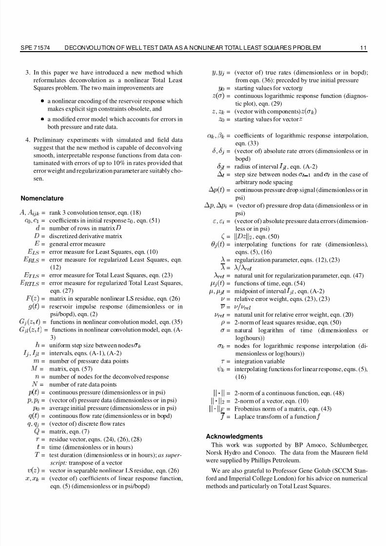
Nomenclature

,

= rank 3 convolution tensor, eqn. (18)

,

= coefficients in initial response

, eqn. (51)

= number of rows in matrix

= discretized derivative matrix

= general error measure

= error measure for Least Squares, eqn. (10)

= error measure for regularized Least Squares, eqn.

(12)

= error measure for Total Least Squares, eqn. (23)

= error measure for regularized Total Least Squares,

eqn. (27)

= matrix in separable nonlinear LS residue, eqn. (26)

= reservoir impulse response (dimensionless or in

psi/bopd), eqn. (2)

= functions in nonlinear convolution model, eqn. (35)

= functions in nonlinear convolution model, eqn. (A-

3)

= uniform step size between nodes

,

= intervals, eqns. (A-1), (A-2)

= number of pressure data points

= matrix, eqn. (57)

= number of nodes for the deconvolved response

= number of rate data points

= continuous pressure (dimensionless or in psi)

,

= (vector of) pressure data (dimensionless or in psi)

= average initial pressure (dimensionsless or in psi)

= continuous flow rate (dimensionless or in bopd)

,

= (vector of) discrete flow rates

= matrix, eqn. (7)

= residue vector, eqns. (24), (26), (28)

= time (dimensionless or in hours)

= test duration (dimensionless or in hours); as super-

script: transpose of a vector

= vector in separable nonlinear LS residue, eqn. (26)

,

= (vector of) coefficients of linear response function,eqn. (5) (dimensionless or in psi/bopd)

,

= (vector of) true rates (dimensionless or in bopd);

from eqn. (36): preceded by true initial pressure

= starting values for vector

= continuous logarithmic response function (diagnos-tic plot), eqn. (29)

,

= (vector with components)

= starting values for vector

,

= coefficients of logarithmic response interpolation,

eqn. (33)

Æ

,Æ

= (vector of) absolute rate errors (dimensionless or in

bopd)

Æ

= radius of interval

, eqn. (A-2)

= step size between nodes

and

in the case of

arbitrary node spacing

= continuous pressure drop signal (dimensionless or inpsi)

,

= (vector of) pressure drop data (dimensionless or in

psi)

,

= (vector of) absolute pressure data errors (dimension-

less or in psi)

=

, eqn. (50)

= interpolating functions for rate (dimensionless),

eqns. (5), (16)

= regularization parameter, eqns. (12), (23)

=

= natural unit for regularization parameter, eqn. (47)

= functions of time, eqn. (54)

,

= midpoint of interval

, eqn. (A-2)

= relative error weight, eqns. (23), (23)

=

= natural unit for relative error weight, eqn. (20)

= 2-norm of least squares residue, eqn. (50)

= natural logarithm of time (dimensionless or

log(hours))

= nodes for logarithmic response interpolation (di-

mensionless or log(hours))

= integration variable

= interpolating functions for linear response, eqns. (5),

(16)

= 2-norm of a continuous function, eqn. (48)

= 2-norm of a vector, eqn. (10)

= Frobenius norm of a matrix, eqn. (43)

= Laplace transform of a function

Acknowledgments

This work was supported by BP Amoco, Schlumberger,

Norsk Hydro and Conoco. The data from the Maureen field

were supplied by Phillips Petroleum.

We are also grateful to Professor Gene Golub (SCCM Stan-

ford and Imperial College London) for his advice on numericalmethods and particularly on Total Least Squares.




References

1. R. G. Agarwal, R. Al-Hussainy, and H. J. J. Ramey. An investi-

gation of Wellbore Storage and Skin Effect in Unsteady LiquidFlow. I: Analytical Treatment. SPE Journal, Sept. 1970:279–

290, 1970. Paper SPE 2466.

2. B. Baygun, F. J. Kuchuk, and O. Arikan. Deconvolution Under

Normalized Autocorrelation Constraints. SPE Journal, 2:246–

253, 1997. Paper SPE 28405.

3. Bjorck, A. Numerical methods for Least Squares problems. So-

ciety for Industrial and Applied Mathematics (SIAM), Philadel-

phia, 1996.

4. D. Bourdet, J. A. Ayoub, and Y. M. Pirard. Use of pressure

derivative in well-test interpretation. SPE Formation Evaluation,

June 1989:293–302, 1989. Paper SPE 12777.

5. M. J. Bourgeois and R. N. Horne. Well-Test-Model Recogni-

tion with Laplace Space. SPE Formation Evaluation, March

1993:17–25, 1993. Paper SPE 22682.

6. K. H. Coats, L. A. Rapoport, J. R. McCord, and W. P. Drews.

Determination of Aquifer Influence Functions From Field Data.

Trans. SPE (AIME), 231:1417–24, 1964.

7. S. Daungkaew, F. Hollaender, and A. C. Gringarten. Frequently

Asked Questions in Well Test Analysis. SPE Annual Technical

Conference and Exhibition, Dallas, Texas, Oct. 1–4, 2000. Paper

SPE 63077.

8. C. W. Dong. A regularization method for the numerical inver-

sion of the Laplace transform. SIAM J. Numer. Anal., 30:759–73,

1993.

9. G. H. Golub, M. Heath, and G. Wahba. Generalized Cross-

Validation as a Method for Choosing a Good Ridge Parameter.

Technometrics, 21:215–223, 1979.10. G. H. Golub and C. F. van Loan. Matrix Computations. The

Johns Hopkins University Press, Baltimore, third edition, 1996.

11. P. C. Hansen and D. P. O’Leary. The use of the L-curve in the

regularization of discrete ill-posed problems. SIAM J. Scientific

Computing, 15:1487–1503, 1993.

12. F. J. Kuchuk, R. G. Carter, and L. Ayestaran. Deconvolution of

Wellbore Pressure and Flow Rate. SPE Formation Evaluation,

March 1990:53–59, 1990. Paper SPE 13960.

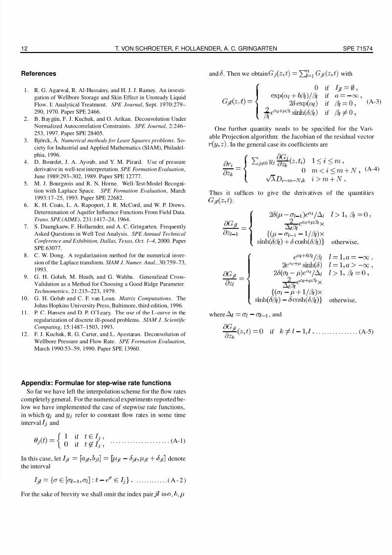
Appendix: Formulae for step-wise rate functions

So far we have left the interpolation scheme for the flow ratescompletely general. For the numerical experiments reported be-

low we have implemented the case of stepwise rate functions,

in which

and

refer to constant flow rates in some time

interval

and

if

if

. . . . . . . . . . . . . . . . . . . . . (A-1)

In this case, let

Æ

Æ

denote

the interval

. . . . . . . . . . . . ( A - 2 )

For the sake of brevity we shall omit the index pair in , ,

andÆ

. Then we obtain

with

if

if

Æ

if

Æ

if

(A-3)

One further quantity needs to be specified for the Vari-

able Projection algorithm: the Jacobian of the residual vector

. In the general case its coefficients are

(A-4)

Thus it suffices to give the derivatives of the quantities

:

Æ

Æ

Æ Æ

otherwise,

Æ

Æ

Æ

Æ Æ

otherwise,

where

, and

if

. . . . . . . . . . . . . . . (A-5)

deconvolution of well test data as a nonlinear total least squares problem

Documents