Deep Learning Statistical Arbitrage∗

Jorge Guijarro-Ordonez† Markus Pelger‡ Greg Zanotti§

July 27, 2021

Abstract

Statistical arbitrage identifies and exploits temporal price differences between similar as-

sets. We propose a unifying conceptual framework for statistical arbitrage and develop a novel

deep learning solution, which finds commonality and time-series patterns from large panels in a

data-driven and flexible way. First, we construct arbitrage portfolios of similar assets as resid-

ual portfolios from conditional latent asset pricing factors. Second, we extract the time series

signals of these residual portfolios with one of the most powerful machine learning time-series

solutions, a convolutional transformer. Last, we use these signals to form an optimal trading

policy, that maximizes risk-adjusted returns under constraints. We conduct a comprehensive

empirical comparison study with daily large cap U.S. stocks. Our optimal trading strategy

obtains a consistently high out-of-sample Sharpe ratio and substantially outperforms all bench-

mark approaches. It is orthogonal to common risk factors, and exploits asymmetric local trend

and reversion patterns. Our strategies remain profitable after taking into account trading fric-

tions and costs. Our findings suggest a high compensation for arbitrageurs to enforce the law

of one price.

Keywords: statistical arbitrage, pairs trading, machine learning, deep learning, big data, stock

returns, convolutional neural network, transformer, attention, factor model, market efficiency,

investment.

JEL classification: C14, C38, C55, G12

∗We thank Jose Blanchet, Marcelo Fernandes, Kay Giesecke, Marcelo Medeiros and George Papanicolaou and seminarand conference participants at the Meeting of the Brazilian Finance Society, World Online Seminars on Machine Learning inFinance, NVIDIA AI Webinar, Vanguard Academic Seminar and the Western Conference on Mathematical Finance for helpfulcomments. We thank MSCI for generous research support.†Stanford University, Department of Mathematics, Email: jguiord@stanford.edu.‡Stanford University, Department of Management Science & Engineering, Email: mpelger@stanford.edu.§Stanford University, Department of Management Science & Engineering, Email: gzanotti@stanford.edu.

I. Introduction

Statistical arbitrage is one of the pillars of quantitative trading, and has long been used by

hedge funds and investment banks. The term statistical arbitrage encompasses a wide variety of

investment strategies, which identify and exploit temporal price differences between similar assets

using statistical methods. Its simplest form is known as “pairs trading”. Two stocks are selected

that are “similar”, usually based on historical co-movement in their price time-series. When the

spread between their prices widens, the arbitrageur sells the winner and buys the loser. If their

prices move back together, the arbitrageur will profit. While Wall Street has developed a plethora

of proprietary tools for sophisticated arbitrage trading, there is still a lack of understanding of

how much arbitrage opportunity is actually left in financial markets. In this paper we answer the

two key questions around statistical arbitrage: What are the important elements of a successful

arbitrage strategy and how much realistic arbitrage is in financial markets?

Every statistical arbitrage strategy needs to solve the following three fundamental problems:

Given a large universe of assets, what are long-short portfolios of similar assets? Given these

portfolios, what are time series signals that indicate the presence of temporary price deviations?

Last, but not least, given these signals, how should an arbitrageur trade them to optimize a trading

objective while taking into account possible constraints and market frictions? Each of these three

questions poses substantial challenges, that prior work has only partly addressed. First, it is a

hard problem to find long-short portfolios for all stocks as it is a priori unknown what constitutes

“similarity”. This problem requires considering all the big data available for a large number of

assets and times, including not just conventional return data but also exogenous information like

asset characteristics. Second, extracting the right signals requires detecting flexibly all the relevant

patterns in the noisy, complex, low-sample-size time series of the portfolio prices. Last but not

least, optimal trading rules on a multitude of signals and assets are complicated and depend on

the trading objective. All of these challenges fundamentally require flexible estimation tools that

can deal with many variables. It is a natural idea to use machine learning techniques like deep

neural networks to deal with the high dimensionality and complex functional dependencies of the

problem. However, our problem is different from the usual prediction task, where machine learning

tools excel. We show how to optimally design a machine learning solution to our problem that

leverages the economic structure and objective.

In this paper, we propose a unifying conceptual framework that generalizes common approaches

to statistical arbitrage. Statistical arbitrage can be decomposed into three fundamental elements:

(1) arbitrage portfolio generation, (2) arbitrage signal extraction and (3) the arbitrage allocation

decision given the signal. By decomposing different methods into their arbitrage portfolio, signal

and allocation element, we can compare different methods and study which components are the most

relevant for successful trading. For each step we develop a novel machine learning implementation,

which we compare with conventional methods. As a result, we construct a new deep learning

statistical arbitrage approach. Our new approach constructs arbitrage portfolios with a conditional

latent factor model, extracts the signals with the currently most successful machine learning time-

1

series method and maps them into a trading allocation with a flexible neural network. These

components are integrated and optimized over a global economic objective, which maximizes the

risk-adjusted return under constraints. Empirically, our general model outperforms out-of-sample

the leading benchmark approaches and provides a clear insight into the structure of statistical

arbitrage.

To construct arbitrage portfolios, we introduce the economically motivated asset pricing per-

spective to create them as residuals relative to asset pricing models. This perspective allows us to

take advantage of the recent developments in asset pricing and to also include a large set of firm

characteristics in the construction of the arbitrage portfolios. We use fundamental risk factors and

conditional and unconditional statistical factors for our asset pricing models. Similarity between

assets is captured by similar exposure to those factors. Arbitrage Pricing Theory implies that, with

an appropriate model, the corresponding factor portfolios represent the “fair price” of each of the

assets. Therefore, the residual portfolios relative to the asset pricing factors capture the tempo-

rary deviations from the fair price of each of the assets and should only temporally deviate from

their long-term mean. Importantly, the residuals are tradeable portfolios, which are only weakly

cross-sectionally correlated, and close to orthogonal to firm characteristics and systematic factors.

These properties allow us to extract a stationary time-series model for the signal.

To detect time series patterns and signals in the residual portfolios, we introduce a filter perspec-

tive and estimate them with a flexible data-driven filter based on convolutional networks combined

with transformers. In this way, we do not prescribe a potentially misspecified function to extract the

time series structure, for example, by estimating the parameters of a given parametric time-series

model, or the coefficients of a decomposition into given basis functions, as in conventional methods.

Instead, we directly learn in a data-driven way what the optimal pattern extraction function is for

our trading objective. The convolutional transformer is the ideal method for this purpose. Convo-

lutional neural networks are the state-of-the-art AI method for pattern recognition, in particular

in computer vision. In our case they identify the local patterns in the data and may be thought

as a nonlinear and learnable generalization of conventional kernel-based data filters. Transformer

networks are the most successful AI model for time series in natural language processing. In our

model, they combine the local patterns to global time-series patterns. Their combination results in

a data-driven flexible time-series filter that can essentially extract any complex time-series signal,

while providing an interpretable model.

To find the optimal trading allocation, we propose neural networks to map the arbitrage signals

into a complex trading allocation. This generalizes conventional parametric rules, for example fixed

rules based on thresholds, which are only valid under strong model assumptions and a small signal

dimension. Importantly, these components are integrated and optimized over a global economic

objective, which maximizes the risk-adjusted return under constraints. This allows our model

to learn the optimal signals and allocation for the actual trading objective, which is different

from a prediction objective. The trading objective can maximize the Sharpe ratio or expected

return subject to a risk penalty, while taking into account constraints important to real investment

2

managers, such as restricting turnover, leverage, or proportion of short trades.

Our comprehensive empirical out-of-sample analysis is based on the daily returns of roughly the

550 largest and most liquid stocks in the U.S. from 1998 to 2016. We estimate the out-of-sample

residuals on a rolling window relative to the empirically most important factor models. These

are observed fundamental factors, for example the Fama-French 5 factors and price trend factors,

locally estimated latent factors based on principal component analysis (PCA) or locally estimated

conditional latent factors that include the information in 46 firm-specific characteristics and are

based on the Instrumented PCA (IPCA) of Kelly et al. (2019). We extract the trading signal with

one of the most successful parametric models, based on the mean-reverting Ornstein-Uhlenbeck

process, a frequency decomposition of the time-series with a Fourier transformation and our novel

convolutional network with transformer. Finally, we compare the trading allocations based on

parametric or nonparametric rules estimated with different risk-adjusted trading objectives.

Our empirical main findings are five-fold. First, our deep learning statistical arbitrage model

substantially outperforms all benchmark approaches out-of-sample. In fact, our model can achieve

an impressive annual Sharpe ratio larger than four. While respecting short-selling constraints we

can obtain annual out-of-sample mean returns of 20%. This performance is four times better than

one of the best parametric arbitrage models, and twice as good as an alternative deep learning

model without the convolutional transformer filter. These results are particularly impressive as we

only trade the largest and most liquid stocks. Hence, our model establishes a new standard for

arbitrage trading.

Second, the performance of our deep learning model suggests that there is a substantial amount

of short-term arbitrage in financial markets. The profitability of our strategies is orthogonal to

market movements and conventional risk factors including momentum and reversal factors and

does not constitute a risk-premium. Our strategy performs consistently well over the full time

horizon. The model is extremely robust to the choice of tuning parameters, and the period when

it is estimated. Importantly, our arbitrage strategy remains profitable in the presence of realistic

transaction and holdings costs. Assessing the amount of arbitrage in financial markets with un-

conditional pricing errors relative to factor models or with parametric statistical arbitrage models,

severely underestimates this quantity.

Third, the trading signal extraction is the most challenging and separating element among dif-

ferent arbitrage models. Surprisingly, the choice of asset pricing factors has only a minor effect

on the overall performance. Residuals relative to the five Fama-French factors and five locally

estimated principal component factors perform very well with out-of-sample Sharpe ratios above

3.2 for our deep learning model. Five conditional IPCA factors increase the out-of-sample Sharpe

ratio to 4.2, which suggests that asset characteristics provide additional useful information. In-

creasing the number of risk factors beyond five has only a marginal effect. Similarly, the other

benchmark models are robust to the choice of factor model as long as it contains sufficiently many

factors. The distinguishing element is the time-series model to extract the arbitrage signal. The

convolutional transformer doubles the performance relative to an identical deep learning model

3

with a pre-specified frequency filter. Importantly, we highlight that time-series modeling requires a

time-series machine learning approach, which takes temporal dependency into account. An off-the-

shelf nonparametric machine learning method like conventional neural networks, that estimates an

arbitrage allocation directly from residuals, performs substantially worse.

Fourth, successful arbitrage trading is based on local asymmetric trend and reversion patterns.

Our convolutional transformer framework provides an interpretable representation of the underlying

patterns, based on local basic patterns and global “dependency factors”. The building blocks of

arbitrage trading are smooth trend and reversion patterns. The arbitrage trading is short-term

and the last 30 trading days seem to capture the relevant information. Interestingly, the direction

of policies is asymmetric. The model reacts quickly on downturn movements, but more cautiously

on uptrends. More specifically, the “dependency factors” which are the most active in downturn

movements focus only on the most recent 10 days, while those for upward movements focus on the

first 20 days in a 30-day window.

Fifth, time-series-based trading patterns should be extracted from residuals and not directly

from returns. For an appropriate factor model, the residuals are only weakly correlated and close

to stationary in both, the time and cross-sectional dimension. Hence, it is meaningful to extract

a uniform trading pattern, that is based only on the past time-series information, from the resid-

uals. In contrast stock returns are dominated by a few factors, which severely limits the actual

independent time-series information, and are strongly heterogenous due to their variation in firm

characteristics. While the level of stock returns is extremely hard to predict, even with flexible

machine learning methods, residuals capture relative movements and remove the level component.

These properties make residuals analyzable from a purely time-series based perspective and, unlike

the existing literature, they allow us to incorporate alternative data into the portfolio construction

process. This also highlights a fundamental difference with most of the existing financial machine

learning literature: We do not use characteristics to get features for prediction, but rather to

generate new data orthogonal to these features.

Related Literature

Our paper builds on the classical statistical arbitrage literature, in which the three main prob-

lems of portfolio generation, pattern extraction, and allocation decision have traditionally been

considered independently. Classical statistical methods of generating arbitrage portfolios have

mostly focused on obtaining multiple pairs or small portfolios of assets, using techniques like the

distance method of Gatev et al. (2006), the cointegration approach of Vidyamurthy (2004), or cop-

ulas as in Rad et al. (2016). In contrast, more general methods that exploit large panels of stock

returns include the use of PCA factor models, as in Avellaneda and Lee (2010) and its extension

in Yeo and Papanicolaou (2017), and the maximization of mean-reversion and sparsity statistics as

in d’Aspremont (2011). We include the model of Yeo and Papanicolaou (2017) as the parametric

benchmark model in our study as it has one of the best empirical performances among the class of

parametric models. Our paper paper contributes to this literature by introducing a general asset

4

pricing perspective to obtain the arbitrage portfolios as residuals. This allows us to take advantage

of conditional asset pricing models, that include time-varying firm characteristics in addition to the

return time-series, and provides a more disciplined, economically motivated approach. The signal

extraction step for these models assumes parametric time series models for the arbitrage portfolios,

whereas the allocations are often decided from the estimated parameters by using stochastic con-

trol methods or given threshold rules and one-period optimizations. Some representative papers

of the first approach include Jurek and Yang (2007), Mudchanatongsuk et al. (2008), Cartea and

Jaimungal (2016), Lintilhac and Tourin (2016) and Leung and Li (2015), whereas the second one is

illustrated by Elliott et al. (2005) and Yeo and Papanicolaou (2017). Both approaches are special

cases of our more general framework. Mulvey et al. (2020) and Kim and Kim (2019) are exam-

ples of including machine learning elements within the parametric statistical arbitrage framework,

by either solving a stochastic control problem with neural networks or estimating a time-varying

threshold rule with reinforcement learning.

Our paper is complementary to the emerging literature that uses machine learning methods for

asset pricing. While the asset pricing literature aims to explain the risk premia of assets, our focus is

on the residual component which is not explained by the asset pricing models. Chen et al. (2019),

Bryzgalova et al. (2019) and Kozak et al. (2020) estimate the stochastic discount factor (SDF),

which explains the risk premia of assets, with deep neural networks, decision trees or elastic net

regularization. These papers employ advanced statistical methods to solve a conditional method of

moment problem in the presence of many variables. The workhorse models in equity asset pricing

are based on linear factor models exemplified by Fama and French (1993, 2015). Recently, new

methods have been developed to extract statistical asset pricing factors from large panels with

various versions of principal component analysis (PCA). The Risk-Premium PCA in Lettau and

Pelger (2020a,b) includes a pricing error penalty to detect weak factors that explain the cross-

section of returns. The high-frequency PCA in Pelger (2020) uses high-frequency data to estimate

local time-varying latent risk factors and the Instrumented PCA (IPCA) of Kelly et al. (2019)

estimates conditional latent factors by allowing the loadings to be functions of time-varying asset

characteristics. Gu et al. (2021) generalize IPCA to allow the loadings to be nonlinear functions of

characteristics.

Our paper is related to the growing literature on return prediction with machine learning meth-

ods, which has shown the benefits of regularized flexible methods. In their pioneering work Gu

et al. (2020) conduct a comparison of machine learning methods for predicting the panel of in-

dividual U.S. stock returns based on the asset-specific characteristics and economic conditions in

the previous period. In a similar spirit, Bianchi et al. (2019) predict bond returns and Freyberger

et al. (2020) use different methods for predicting stock returns. This literature is fundamentally

estimating the risk premia of assets, while our focus is on understanding and exploiting the tem-

poral deviations thereof. This different goal is reflected in the different methods that are needed.

These return predictions estimate a nonparametric model between current returns and large set of

covariates from the last period, but do not estimate a time-series model. In contrast, the important

5

challenge that we solve is to extract a complex time-series pattern. A related stream of this litera-

ture forecasts returns using past returns, generally followed by some long-short investment policy

based on the prediction. For example, Krauss et al. (2017) use various machine learning methods

for this type of prediction.1 However, they use general nonparametric function estimates, which

are not specifically designed for time-series data. Lim and Zohren (2020) show that it is important

for machine learning solutions to explicitly account for temporal dependence when they are applied

to time-series data. Forecasting returns and building a long-short portfolio based on the prediction

is different from statistical arbitrage trading as it combines a risk premium and potential arbitrage

component. It is not based on temporary price differences and also in general not orthogonal to

common risk factors and market movements. In this paper we highlight the challenge of inferring

complex time-series information and argue that using returns directly as an input to a time-series

machine learning method, is suboptimal as returns are dominated by a few factor time-series and

heterogeneous due to cross-sectionally and time-varying characteristics. In contrast, appropriate

residuals are locally stationary and hence allow the extraction of a complex time-series pattern.

Naturally, our work overlaps with the literature on using machine learning tools for investment.

The SDF estimated by asset pricing models, like in Chen et al. (2019) and Bryzgalova et al. (2019),

directly maps into a conditionally mean-variance efficient portfolio and hence an attractive invest-

ment opportunity. However, by construction this investment portfolio is not orthogonal but fully

exposed to systematic risk, which is exactly the opposite for an arbitrage portfolio. Prediction

approaches also imply investment strategies, typically long-short portfolios based on the predic-

tion signal. However, estimating a signal with a prediction objective, is not necessarily providing

an optimal signal for investment. Bryzgalova et al. (2019) and Chen et al. (2019) illustrate that

machine learning models that use a trading objective can result in a substantially more profitable

investment than models that estimate a signal with a prediction objective, while using the same

information as input and having the same flexibility. This is also confirmed in Cong et al. (2020),

who use an investment objective and reinforcement learning to construct machine learning invest-

ment portfolios. Our paper contributes to this literature by estimating investment strategies, that

are orthogonal to systematic risk and are based on a trading objective with constraints.

Finally, our approach is also informed by the recent deep learning for time series literature. The

transformer method was first introduced in the groundbreaking paper by Vaswani et al. (2017). We

are the first to bring this idea into the context of statistical arbitrage and adopt it to the economic

problem.

II. Model

The fundamental problem of statistical arbitrage consists of three elements: (1) The identifica-

tion of similar assets to generate arbitrage portfolios, (2) the extraction of time-series signals for

the temporary deviations of the similarity between assets and (3) a trading policy in the arbitrage

1Similar studies include Fischer et al. (2019), Chen et al. (2018), Huck (2009), and Dunis et al. (2006).

6

portfolios based on the time-series signals. We discuss each element separately.

A. Arbitrage portfolios

We consider a panel of excess returns Rn,t, that is the return minus risk free rate of stock

n = 1, ..., Nt at time t = 1, ..., T . The number of available assets at time t can be time-varying.

The excess return vector of all assets at time t is denoted as Rt =(R1,t · · · RNt,t

)>.

We use a general asset pricing model to identify similar assets. In this context, similarity is

defined as the same exposure to systematic risk, which implies that assets with the same risk

exposure should have the same fundamental value. We assume that asset returns can be modeled

by a conditional factor model:

Rn,t = β>n,t−1Ft + εn,t.

The K factors F ∈ RT×K capture the systematic risk, while the risk loadings βt−1 ∈ RNt×K can be

general functions of the information set at time t− 1 and hence can be time-varying. This general

formulation includes the empirically most successful factor models. In our empirical analysis we

will include observed traded factors, e.g. the Fama-French 5 factor model, latent factors based on

the principal components analysis (PCA) of stock returns and conditional latent factors estimated

with Instrumented Principal Component Analysis (IPCA).

Without loss of generality, we can treat the factors as excess returns of traded assets. Either

the factors are traded, for example a market factor, in which case we include them in the returns

Rt. Otherwise, we can generate factor mimicking portfolios by projecting them on the asset space,

as for example with latent factors:

Ft = wFt−1>Rt.

We define arbitrage portfolio as residual portfolios εn,t = Rn,t − β>n,t−1Ft. As factors are traded

assets, the arbitrage portfolio is itself a traded portfolio: Hence, the residual portfolio equals

εt = Rt − βt−1wFt−1>Rt =

(INt − βt−1w

Ft−1>)︸ ︷︷ ︸

Φt−1

Rt = Φt−1Rt. (1)

Arbitrage portfolios are projections on the return space that annihilate systematic asset risk. For

an appropriate asset pricing model, the residual portfolios should not earn a risk premium. This

is the fundamental assumption behind any arbitrage argument. As deviations from a mean of zero

have to be temporary, arbitrage trading bets on the mean revision of the residuals. In particular,

for an appropriate factor model the residuals will have the following properties:

1. The unconditional mean of the arbitrage portfolios is zero: E[εn,t] = 0.

2. The arbitrage portfolios are only weakly cross-sectionally dependent.

7

We denote by Ft the filtration generated by the returns Rt, which include the factors, and the

information set that captures the risk exposure βt, which is typically based on asset specific char-

acteristics or past returns.

B. Arbitrage signal

The arbitrage signal is extracted from the time-series of the arbitrage portfolios. These time-

series signals are the input for a trading policy. An example for an arbitrage signal would be a

parametric model for mean reversion that is estimated for each arbitrage portfolio. The trading

strategy for each arbitrage portfolio would depend on its speed of mean reversion and its deviation

from the long run mean. More generally, the arbitrage signal is the estimation of a time-series model,

which can be parametric or nonparametric. An important class of models are filtering approaches.

Conceptually, time-series models are multivariate functional mappings between sequences which

take into account the temporal order of the elements and potentially complex dependencies between

the elements of the input sequence.

We apply the signal extraction to the time-series of the last L lagged residuals, which we denote

in vector notation as

εLn,t−1 :=(εn,t−L · · · εn,t−1

).

The arbitrage signal function is a mapping θ ∈ Θ from RL to Rp, where Θ defines an appropriate

function space:

θ(·) : εLn,t−1 → θn,t−1.

The signals θn,t−1 ∈ Rp for the arbitrage portfolio n at time t only depend on the time-series

of lagged returns εLn,t−1. Note that the dimensionality of the signal can be the same as for the

input sequence. Formally, the function θ is a mapping from the filtration F ε,Ln,t−1 generated by

εLn,t−1 into the filtration Fθn,t−1 generated by θn,t−1 and Fθn,t−1 ⊆ Fε,Ln,t−1. We use the notation

of evaluating functions elementwise, that is θ(εLt−1) =(θ1,t−1 · · · θNt,t−1

)= θt−1 ∈ RNt with

εLt−1 =(ε1,t−1 · · · εNt,t−1

).

The arbitrage signal θn,t−1 is a sufficient statistic for the trading policy; that is, all relevant

information for trading decisions is summarized in it. This also implies that two arbitrage portfolios

with the same signal get the same weight in the trading strategy. More formally, this means that the

arbitrage signal defines equivalence classes for the arbitrage portfolios. The most relevant signals

summarize reversal patterns and their direction with a small number of parameters. A potential

trading policy could be to hold long positions in residuals with a predicted upward movement and

go short in residuals that are in a downward cycle.

This problem formulation makes two implicit assumptions. First, the residual time-series follow

a stationary distribution conditioned on its lagged returns. This is a very general framework that

8

includes the most important models for financial time-series. Second, the first L lagged returns are

a sufficient statistic to obtain the arbitrage signal θn,t−1. This reflects the motivation that arbitrage

is a temporary deviation of the fair price. The lookback window can be chosen to be arbitrarily

large, but in practice it is limited by the availability of lagged returns.

C. Arbitrage trading

The trading policy assigns an investment weight to each arbitrage portfolio based on its signal.

The allocation weight is the solution to an optimization problem, which models a general risk-return

tradeoff and can also include trading frictions and constraints. An important case are mean-variance

efficient portfolios with transaction costs and short sale constraints.

An arbitrage allocation is a mapping from Rp to R in a function class W , that assigns a weight

wεn,t−1 for the arbitrage portfolio εn,t−1 in the investment strategy using only the arbitrage signal

θn,t:

wε : θn,t−1 → wεn,t−1.

Given a concave utility function U(·), the allocation function is the solution to

maxwε∈W ,θ∈Θ

Et−1

[U(wRt−1Rt

)](2)

s.t. wRt−1 =wεt−1

>Φt−1

‖wεt−1>Φt−1‖1

and wεt−1 = wε(θ(εLt−1)). (3)

In the presence of trading costs, we calculate the expected utility of the portfolio net return by

subtracting from the portfolio return wRt−1Rt the trading costs that are associated with the stock

allocation wRt−1. The trading costs can capture the transaction costs from frequent rebalancing and

the higher costs of short selling compared to long positions. The stock weights wRt−1 are normalized

to add up to one in absolute value, which implicitly imposes a leverage constraint. The conditional

expectation uses the general filtration Ft−1.

This is a combined optimization problem, which simultaneously solves for the optimal allocation

function and arbitrage signal function. As the weight is a composition of the two functions, i.e.

wεt−1 = wε(θ(εLt−1)), the decomposition into a signal and allocation function is in general not

uniquely identified. This means there can be multiple representations of θ and wε, that will result

in the same trading policy. We use a decomposition that allows us to compare the problem to

classical arbitrage approaches, for which this separation is uniquely identified. The key feature of

the signal function θ is that it models a time-series, that means it is a mapping that explicitly models

the temporal order and the dependency between the elements of εLt−1. The allocation function wε

can be a complex nonlinear function, but does not explicitly model time-series behavior. This

means that wε is implicitly limited in the dependency patterns of its input elements that it can

capture.

9

We will consider arbitrage trading that maximizes the Sharpe ratio or achieves the highest

average return for a given level of variance risk. More specifically we will solve for

maxwε∈W ,θ∈Θ

E

[wRt−1

>Rt

]√

Var(wRt−1>Rt)

or maxwε∈W ,θ∈Θ

E[wRt−1>Rt]− γVar(wRt−1

>Rt) (4)

s.t. wRt−1 =wεt−1

>Φt−1

‖wεt−1>Φt−1‖1

and wεt−1 = wε(θ(εLt−1)). (5)

for some risk aversion parameter γ. We will consider this formulation with and without trading

costs.2

Many relevant models estimate the signal and allocation function separately. The arbitrage

signals can be estimated as the parameters of a parametric time-series model, the serial moments

for a given stationary distribution or a time-series filter. In these cases, the signal estimation solves

a separate optimization problem as part of the estimation. Given the signals, the allocation function

is the solution of

maxwε∈W

Et−1

[U(wRt−1Rt

)]s.t. wRt−1 =

wε(θt−1)>Φt−1

‖wε(θt−1)>Φt−1‖1. (6)

We provide an extensive study of the importance of the different elements in statistical arbitrage

trading. We find that the most important driver for profitable portfolios is the arbitrage signal

function; that is, a good model to extract time-series behavior and to time the predictable mean

reversion patterns is essential. The arbitrage portfolios of asset pricing models that are sufficiently

rich result in roughly the same performance. Once an informative signal is extracted, parametric

and nonparametric allocation functions can take advantage of it. We find that the key element is

to consider a sufficiently general class of functions Θ for the arbitrage signal and to estimate the

signal that is the most relevant for trading. In other words, the largest gains in statistical arbitrage

come from flexible time-series signals θ and a joint optimization problem.

D. Models for Arbitrage Signal and Allocation Functions

In this section we introduce different functional models for the signal and allocation functions.

They range from the most restrictive assumptions for simple parametric models to the most flexible

model, which is our sophisticated deep neural network architecture. The general problem is the

estimation of a signal and allocation function given the residual time-series. Here, we take the

residual returns as given, i.e. we have selected an asset pricing model. In order to illustrate the

key elements of the allocation functions, we consider trading the residuals directly. Projecting the

residuals back into the original return space is identical for the different methods and discussed in

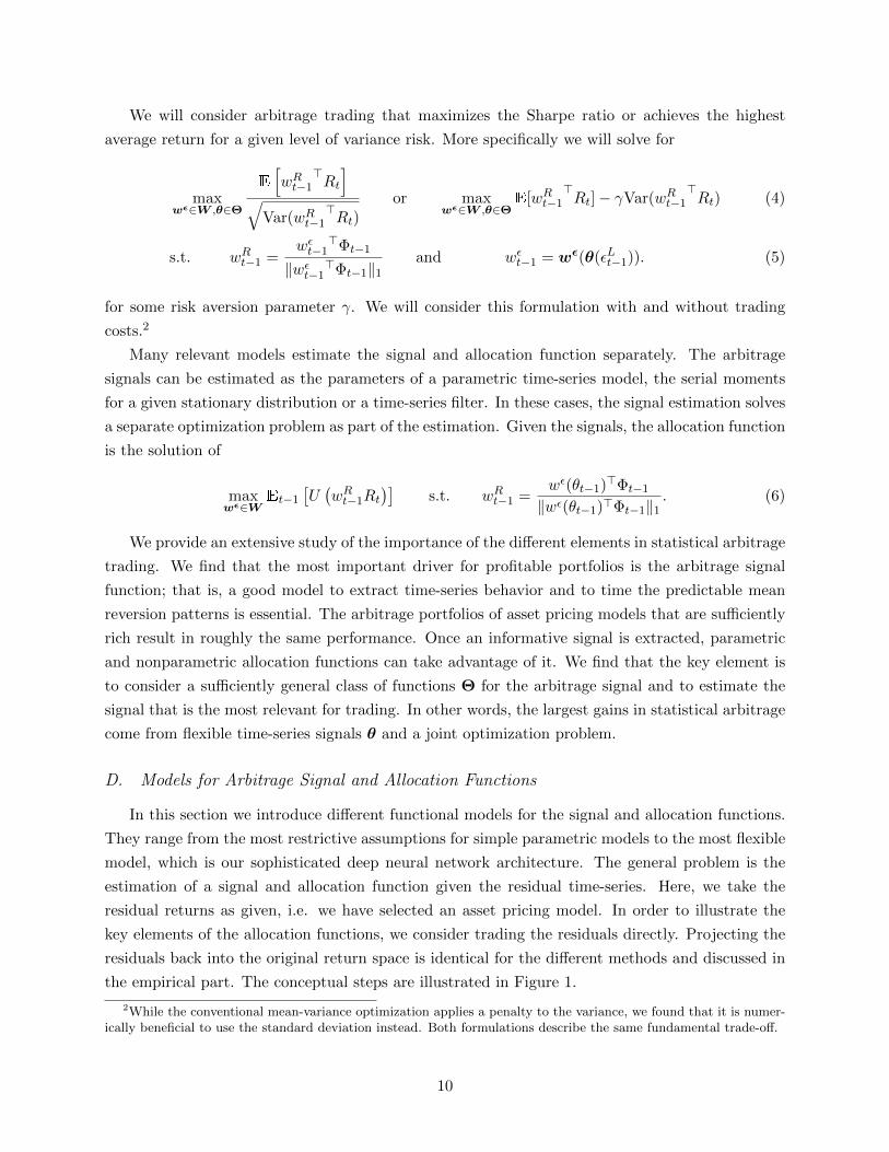
the empirical part. The conceptual steps are illustrated in Figure 1.

2While the conventional mean-variance optimization applies a penalty to the variance, we found that it is numer-ically beneficial to use the standard deviation instead. Both formulations describe the same fundamental trade-off.

10

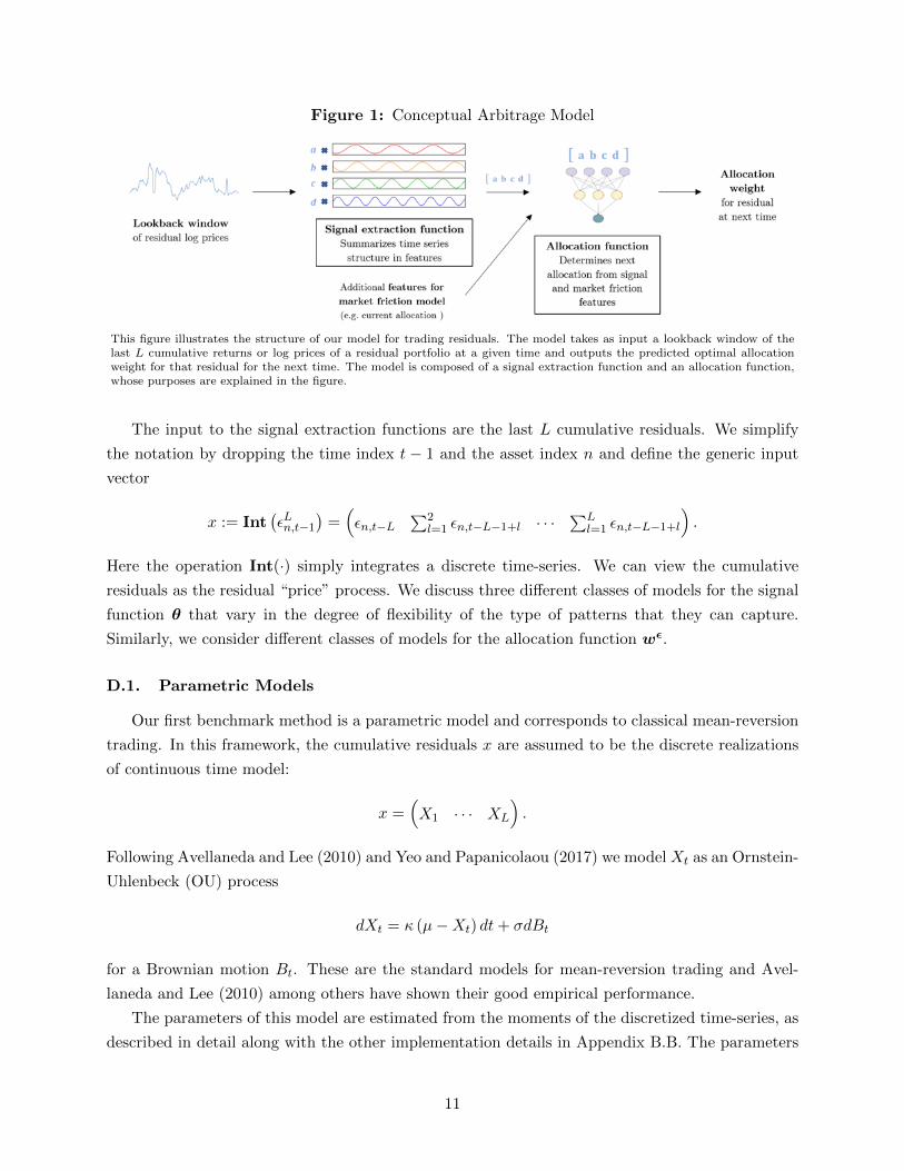
Figure 1: Conceptual Arbitrage Model

This figure illustrates the structure of our model for trading residuals. The model takes as input a lookback window of thelast L cumulative returns or log prices of a residual portfolio at a given time and outputs the predicted optimal allocationweight for that residual for the next time. The model is composed of a signal extraction function and an allocation function,whose purposes are explained in the figure.

The input to the signal extraction functions are the last L cumulative residuals. We simplify

the notation by dropping the time index t − 1 and the asset index n and define the generic input

vector

x := Int(εLn,t−1

)=(εn,t−L

∑2l=1 εn,t−L−1+l · · ·

∑Ll=1 εn,t−L−1+l

).

Here the operation Int(·) simply integrates a discrete time-series. We can view the cumulative

residuals as the residual “price” process. We discuss three different classes of models for the signal

function θ that vary in the degree of flexibility of the type of patterns that they can capture.

Similarly, we consider different classes of models for the allocation function wε.

D.1. Parametric Models

Our first benchmark method is a parametric model and corresponds to classical mean-reversion

trading. In this framework, the cumulative residuals x are assumed to be the discrete realizations

of continuous time model:

x =(X1 · · · XL

).

Following Avellaneda and Lee (2010) and Yeo and Papanicolaou (2017) we model Xt as an Ornstein-

Uhlenbeck (OU) process

dXt = κ (µ−Xt) dt+ σdBt

for a Brownian motion Bt. These are the standard models for mean-reversion trading and Avel-

laneda and Lee (2010) among others have shown their good empirical performance.

The parameters of this model are estimated from the moments of the discretized time-series, as

described in detail along with the other implementation details in Appendix B.B. The parameters

11

for each residual process, the last cumulative sum and a goodness of fit measure form the signals

for the Ornstein-Uhlenbeck model:

θOU =(κ µ σ XL R2

).

Following Yeo and Papanicolaou (2017) we also include the goodness of fit parameter R2 as part of

the signal. R2 has the conventional definition of the ratio of squared values explained by the model

normalized by total squared values. If the R2 value is too low, the predictions of the model seem

to be unreliable, which can be taken into account in a trading policy. Hence, for each cumulative

residual vector εLn,t−1 we obtain the signal

θOUn,t−1 =

(κn,t−1 µn,t−1 σn,t−1

∑Ll=1 εn,t−1+l R2

n,t−1

).

Avellaneda and Lee (2010) and Yeo and Papanicolaou (2017) advocate a classical mean-reversion

thresholding rule, which implies the following allocation function3:

wε|OU(θOU

)=

−1 if XL−µ

σ/√

2κ> cthresh and R2 > ccrit

1 if XL−µσ/√

2κ< −cthresh and R2 > ccrit

0 otherwise

The threshold parameters cthresh and ccrit are tuning parameters. The strategy suggests to buy

or sell residuals based on the ratio XL−µσ/√

2κ. If this ratio exceeds a threshold, it is likely that the

process reverts back to its long term mean, which starts the trading. If the R2 value is too low, the

predictions of the model seem to be unreliable, which stops the trading. This will be our parametric

benchmark model. It has a parametric model for both the signal and allocation function.

Figure 2 illustrates this model with an empirical example. In this figure we show the allocation

weights and signals of the Ornstein-Uhlenbeck with threshold model as well as the more flexible

models that we are going to discuss next. The models are estimated on the empirical data, and the

residual is a representative empirical example. In more detail, we consider the residuals from five

IPCA factors and estimate the benchmark models as explained in the empirical Section III.J. The

left subplots display the cumulative residual process along with the out-of-sample allocation weights

wεl that each model assigns to this specific residual. The evaluation of this illustrative example is

a simplification of the general model that we use in our empirical main analysis. In this example,

we consider trading only this specific residual and hence normalize the weights to {−1, 0, 1}. In

our empirical analysis we trade all residuals and map them back into the original stock returns.

The middle column shows the time-series of estimated out-of-sample signals for each model, by

applying the θl arbitrage signal function to the previous L = 30 cumulative returns of the residual.

The right column displays the out-of-sample cumulative returns of trading this particular residual

3The allocation function is derived by maximizing an expected trading profit. This deviates slightly from ourobjective of either maximizing the Sharpe ratio or the expected return subject to a variance penalty. As this is themost common arbitrage trading rule, we include it as a natural benchmark.

12

based on the corresponding allocation weights.

Figure 2: Illustrative Example of Allocation Weights and Signals for Different Methods

(a) Cumulative residuals xl and

allocation weight wε|CNN+Transl

(b) Signal θCNN+Transl

(c) Cumulative returns ofCNN+Trans strategy

(d) Cumulative residual xl and

allocation weight wε|FFTl

(e) Signal θFFTl(f) Cumulative returns of

Fourier+FFN strategy

(g) Cumulative residual xl and

allocation weight wε|OUl

(h) Signal θOUl

(i) Cumulative returns ofOU+Thresh strategy

These plots are an illustrative example of the allocation weights and signals of the Ornstein-Uhlenbeck with Threshold(OU+Thres), Fast Fourier Transform (FFT) with Feedforward Neural Network (FFN), and Convolutional Neural Network(CNN) with Transformer models for a specific cumulative residual. The models are estimated on the empirical data, and theresidual is a representative empirical example. In more detail, we consider the residuals from five IPCA factors and estimatethe benchmark models as explained in Section III.J. The left subplots display the cumulative residual process along with the

out-of-sample allocation weights wε|·l that each model assigns to this specific residual. In this example, we consider trading

only this specific residual and hence normalize the weights to {−1, 0, 1}. The middle column plots show the time-series ofestimated out-of-sample signals for each model, by applying the θ·l arbitrage signal function to the previous L cumulativereturns of the residual. The right column plots display the out-of-sample cumulative returns of trading this particular residualbased on the corresponding allocation weights. We use a rolling lookback window of L = 30 days to estimate the signal andallocation, which we evaluate for the out-of-sample on the next 30 days. The plots only show the out-of-sample period. Theevaluation of this illustrative example is a simplification of the general model that we use in our empirical main analysis,where we trade all residuals and map them back into the original stock returns.

The last row in Figure 2 shows the results for the OU+Threshold model. The cumulative

return of trading this residual is negative, suggesting that the parametric model fails. The residual

time-series with the corresponding allocation weights in subplot (g) explain why. The trading

allocation does not assign a positive weight during the uptrend and wrongly assigns a constant

negative weight, when the residual price process follows a mean-reversion pattern with positive and

13

negative returns. A parametric model can break down if it is misspecified. This is not only the case

for trend patterns, but also if there are multiple mean reversion patterns of different frequencies.

Subplot (h) shows the signal.4 We see that changes in the allocation function are related to sharp

changes in at least one of the signals, but overall, the signal does not seem to represent the complex

price patterns of the residual.

A natural generalization is to allow for a more flexible allocation function given the same time-

series signals. We will consider for all our models also a general feedforward neural network (FFN)

to map the signal into an allocation weight. FFNs are nonparametric estimators that can capture

very general functional relationships.5 Hence, we also consider the additional model that restricts

the signal function, but allows for a flexible allocation function:

wε|OU-FFN(θOU

)= gFFN

(θOU

).

We will show empirically that the gains of a flexible allocation function are minor relative to the

very simple parametric model.

D.2. Pre-Specified Filters

As a generalization of the restrictive parametric model of the last subsection, we consider

more general time-series models. Many relevant time-series models can be formulated as filtering

problems. Filters are transformations of time-series that provide an alternative representation of

the original time-series which emphasizes certain dynamic patterns.

A time-invariant linear filter can be formulated as

θl =L∑j=1

W filterj xj ,

which is a linear mapping from RL into RL with the matrix W filter ∈ RL×L. The estimation

of causal ARMA processes is an example for such filters. A spectral decomposition based on a

frequency filter is the most relevant filter for our problem of finding mean reversion patterns.

A Fast Fourier Transform (FFT) provides a frequency decomposition of the original time-series

and separates the movements into mean reverting processes of different frequencies. FFT applies

the filter WFFTj = e

2πiLj in the complex plane, but for real-valued time-series it is equivalent to

4For better readability we have scaled the parameters of the OU process by a factor of five, but this still representsthe same model as the scaling cancels out in the allocation function. As a minor modification, we use the ratioσ/√

2κ as a signal instead of two individual parameters, as the conventional regression estimator of the OU processdirectly provides the ratio, but requires additional moments for the individual parameters. However, this results inan equivalent presentation of the model as only the ratio enters the allocation function.

5Appendix B.A provides the details for estimating a FFN as a functional mapping gFFN : Rp → R.

14

fitting the following model:

xl = a0 +

L/2−1∑j=1

(aj · cos

(2πj

Ll

)+ bj · sin

(2πj

Ll

))+ aL/2cos (πl) .

The FFT representation is given by coefficients of the trigonometric representation

θFFT =(a0 · · · aL/2 b1 · · · bL/2−1

)∈ RL.

The coefficients al and bl can be interpreted as “loadings” or exposure to long or short-term reversal

patterns. Note that the FFT is an invertible transformation. Hence, it simply represents the original

time-series in a different form without losing any information. It is based on the insight that not

the magnitude of the original data but the relative relationship in a time-series matters.

We use a flexible feedforward neural network for the allocation function

wε|FFT(θFFT

)= gFFN

(θFFT

).

The usual intuition behind filtering is to use the frequency representation to cut off frequencies

that have low coefficients and therefore remove noise in the representation. The FFN is essentially

implementing this filtering step of removing less important frequencies.

We illustrate the model within our running example in Figure 2. The middle row shows the

results for the FFT+FFN model. The cumulative residual in subplot (d) seems to be a combination

of low and high-frequency movements with an initial trend component. The signal in subplot (e)

suggests that the FFT filter seems to capture the low frequency reversal pattern. However, it

misses the high-frequency components as indicated by the simplistic allocation function. The

trading strategy takes a long position for the first half and a short position for the second part.

While this simple allocation results in a positive cumulative return, in this example it neglects the

more complex local reversal patterns.

While the FFT framework is an improvement over the simple OU model as it can deal with

multiple combined mean-reversion patterns of different frequencies, it fails if the data follows a

pattern that cannot be well approximated by a small number of the prespecified basis functions.

For completeness, our empirical analysis will also report the case of a trivial filter, which simply

takes the residuals as signals, and combines them with a general allocation function:

θident(x) = x = θident

wε|FFN(θident

)= gFFN (x) .

This is a good example to emphasize the importance of a time-series model. While FFNs are

flexible in learning low dimensional functional relationships, they are limited in learning a complex

dependency model. For example, the FFN architecture we consider is not sufficiently flexible

15

to learn the FFT transformation and hence has a worse performance on the original time-series

compared to frequency-transformed time-series. While Xiaohong Chen and White (1999) have

shown that FFNs are “universal approximators” of low-dimensional functional relationships, they

also show that FFN can suffer from a curse of dimensionality when capturing complex dependencies

between the input. Although the time domain and frequency domain representations of the input

are equivalent under the Fourier transform, clearly the time-series model implied by the frequency

domain representation allows for a more effective learning of an arbitrage policy. However, the

choice of the pre-specified filter limits the time-series patterns that can be exploited. The solution

is our data driven filter presented in the next section.

D.3. Convolutional Neural Network with Transformer

Our benchmark machine learning model is a Convolutional Neural Network (CNN) combined

with a Transformer. It uses the most advanced state-of-the art machine learning tools tailored to

our problem. Convolutional networks are in fact the most successful networks for computer vision,

i.e. for pattern detection. Transformers have rapidly become the model of choice for sequence

modeling such as Natural Language Processing (NLP) problems, replacing older recurrent neural

network models such as the Long Short-Term Memory (LSTM) network.

The CNN and transformer framework has two key elements: (1) Local filters and (2) the

temporal combination of these local filters. The CNN can be interpreted as a set of data driven

flexible local filters. A transformer can be viewed as a data driven flexible time-series model to

capture complex dependencies between local patterns. We use the CNN+Transformer to generate

the time-series signal. The allocation function is then modeled as a flexible data driven allocation

with an FFN.

The CNN estimates D local filters of size Dsize:

y(0)l =

Dsize∑m=1

W (0)m xl−m+1

for a matrix W (0) ∈ RDsize×D. The local filters are a mapping from x ∈ RL to y(0) ∈ RL×D given

by the convolution y(0) = W (0) ∗ x. Figure 3 shows examples of these local filters for Dsize = 3.

The values of y(0) can be interpreted as the “loadings” or exposure to local basis patterns. For

example, if x represents a global upward trend, its filtered representation should have mainly large

values for the local upward trend filter.

The convolutional mapping can be repeated in multiple layers to obtain a multi-layer CNN.

First, the output of the first layer of the CNN is transformed nonlinearly by applying the ReLU(·)function:

x(1)l,d = ReLU

(y

(0)l,d

):= max(y

(0)l,d , 0).

16

Figure 3: Examples of Local Filters

(a) Upward trend (b) Downward trend (c) Up reversal (d) Down reversal

These figures show the most important local filters estimated for the benchmark model in our empirical analysis. These areprojections of our higher dimensional nonlinear filter from a 2-layer CNN into two-dimensional linear filters.

The second layer is given by a higher dimensional filtering projection:

y(2)l,d =

Dsize∑m=1

D∑j=1

W(1)d,j,mx

(1)l−m+1,j ,

x(2)l,d = ReLU

(y

(1)l,d

).

The final output of the CNN is x ∈ RL×D. Our benchmark model is a 2-layered convolutional

neural network. The number of layers is a hyperparameter selected on the validation data. Figure

4 illustrates the structure of the 2-layer CNN. While this description captures all the conceptual

elements, the actual implementation includes additional details, such as bias terms, instance nor-

malization and residual connection to improve the implementation as explained in Appendix B.C.

Figure 4: Convolutional Network Architecture

This figure shows the structure of our convolutional network. The network takes as input a window of L consecutive dailycumulative returns a residual, and outputs D features for each block of Dsize days. Each of the features is a nonlinear functionof the observations in the block, and captures a common pattern.

For a 1-layer CNN without the final nonlinear transformation, i.e. for a simple local linear filter,

the patterns can be visualized by the vectors W(0)m . In our case of a 2-layer CNN the local filter

can capture more complex patterns as it applies a 3-dimensional weighting scheme in the array

W (1) and nonlinear transformations. In order to visualize the type of patterns, we project the local

17

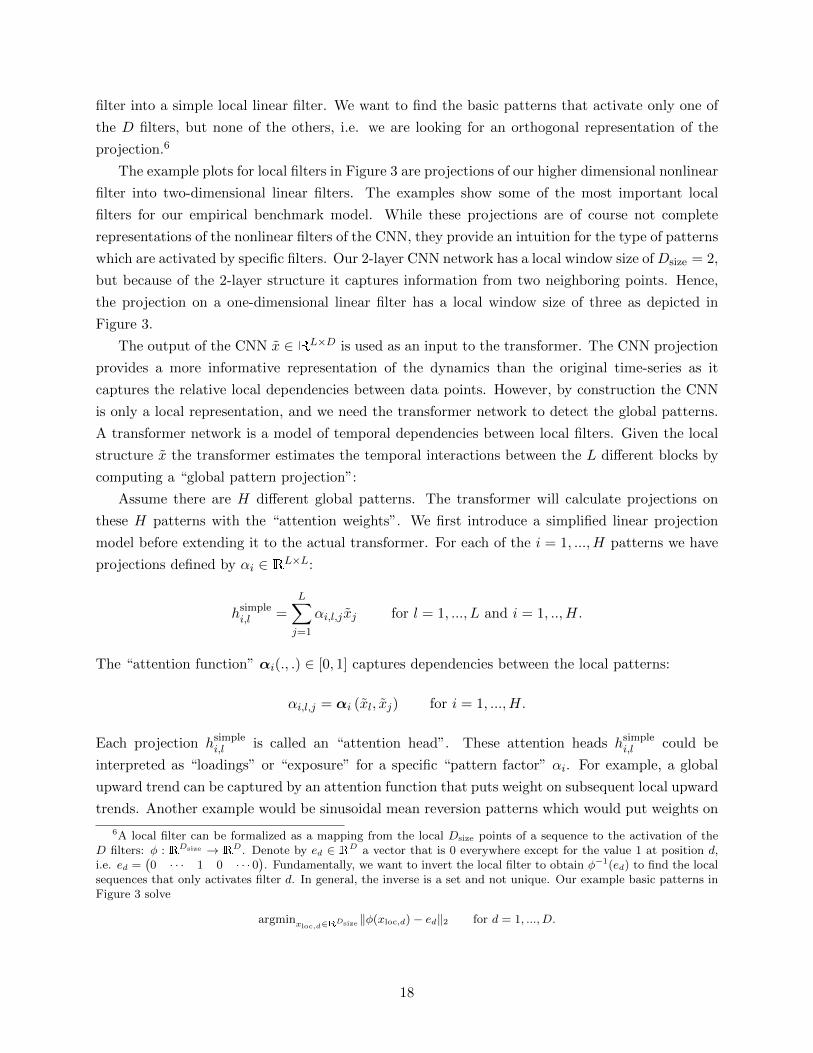
filter into a simple local linear filter. We want to find the basic patterns that activate only one of

the D filters, but none of the others, i.e. we are looking for an orthogonal representation of the

projection.6

The example plots for local filters in Figure 3 are projections of our higher dimensional nonlinear

filter into two-dimensional linear filters. The examples show some of the most important local

filters for our empirical benchmark model. While these projections are of course not complete

representations of the nonlinear filters of the CNN, they provide an intuition for the type of patterns

which are activated by specific filters. Our 2-layer CNN network has a local window size of Dsize = 2,

but because of the 2-layer structure it captures information from two neighboring points. Hence,

the projection on a one-dimensional linear filter has a local window size of three as depicted in

Figure 3.

The output of the CNN x ∈ RL×D is used as an input to the transformer. The CNN projection

provides a more informative representation of the dynamics than the original time-series as it

captures the relative local dependencies between data points. However, by construction the CNN

is only a local representation, and we need the transformer network to detect the global patterns.

A transformer network is a model of temporal dependencies between local filters. Given the local

structure x the transformer estimates the temporal interactions between the L different blocks by

computing a “global pattern projection”:

Assume there are H different global patterns. The transformer will calculate projections on

these H patterns with the “attention weights”. We first introduce a simplified linear projection

model before extending it to the actual transformer. For each of the i = 1, ...,H patterns we have

projections defined by αi ∈ RL×L:

hsimplei,l =

L∑j=1

αi,l,j xj for l = 1, ..., L and i = 1, ..,H.

The “attention function” αi(., .) ∈ [0, 1] captures dependencies between the local patterns:

αi,l,j = αi (xl, xj) for i = 1, ...,H.

Each projection hsimplei,l is called an “attention head”. These attention heads hsimple

i,l could be

interpreted as “loadings” or “exposure” for a specific “pattern factor” αi. For example, a global

upward trend can be captured by an attention function that puts weight on subsequent local upward

trends. Another example would be sinusoidal mean reversion patterns which would put weights on

6A local filter can be formalized as a mapping from the local Dsize points of a sequence to the activation of theD filters: φ : RDsize → R

D. Denote by ed ∈ RD a vector that is 0 everywhere except for the value 1 at position d,i.e. ed =

(0 · · · 1 0 · · · 0

). Fundamentally, we want to invert the local filter to obtain φ−1(ed) to find the local

sequences that only activates filter d. In general, the inverse is a set and not unique. Our example basic patterns inFigure 3 solve

argminxloc,d∈RDsize ‖φ(xloc,d)− ed‖2 for d = 1, ..., D.

18

alternating “curved” local basis patterns. The projection on these weights captures how much a

specific time-series x is exposed to this global pattern. Hence, hsimplei,l measures the exposure to the

global pattern i at time l of the time-series x. Each attention head can focus on a specific global

pattern, which we then combine to obtain our signal.

The fundamental challenge is to learn attention functions that can model complex dependencies.

The crucial innovation in transformers is their modeling of the attention functions αi and attention

heads hi. In order to deal with the high dimensionality of the problem, transformers consider

lower dimensional projections of x into RD/H and use the lower-dimensional scaled dot product

attention mechanism for αi as explained in Appendix B.C. More specifically, each attention head

hi ∈ RL×D/H is based on7 the projected input xW Vi with W V

i ∈ RD×D/H and αi ∈ RL×L:

hi = αixWVi for i = 1, ..,H.

The projection on all global basis patterns h ∈ RL×D/H is given by a weighted linear combination

of the different attention heads

hproj =(h1 · · · hH

)WO

with WO ∈ RD×D. This final projection can, for example, model a combination of a global trend

and mean reversion patterns. In conclusion, hproj represents the time-series in terms of the H

global patterns. This is analogous to a Fourier filter, but without pre-specifying the global patterns

a priori. All parts of the CNN+Transformer network, i.e. the local patterns, the attention functions

and the projections on global patterns, are estimated from the data.

The trading signal θCNN+Trans equals the global pattern projection for the final cumulative

return projection8 hprojL :

θCNN+Trans = hprojL ∈ RH ,

which is then used as input to a time-wise feedforward network allocation function

wε|CNN+Trans(θCNN+Trans

)= gFFN

(θCNN+Trans

).

The separation between signal and allocation is not uniquely identified as we use a joint optimization

problem. We have chosen a separation that maps naturally into the classical examples considered

in the previous subsections. Figure 5 illustrates the transformer network architecture. We have

presented a 1-layer transformer network, which is our benchmark model. The transformed data

7The actual implementation also includes bias terms which we neglect here for simplicity. The Appendix providesthe implementation details.

8In principle, we can use the complete matrix h ∈ RL×D as the signal. However, conceptually the global patternat the end of the time period should be the most relevant for the next realization of the process. We have alsoimplemented a transformer that uses the full matrix, with similar results and the variable importance rankingssuggest that only hL is selected in the allocation function.

19

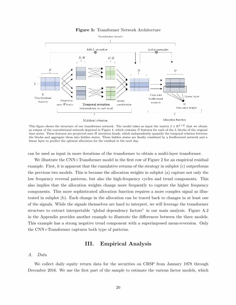
Figure 5: Transformer Network Architecture

This figure shows the structure of our transformer network. The model takes as input the matrix x ∈ RL×D that we obtainas output of the convolutional network depicted in Figure 4, which contains D features for each of the L blocks of the originaltime series. These features are projected onto H attention heads, which independently quantify the temporal relation betweenthe blocks and aggregate them into hidden states. These hidden states are finally combined by a feedforward network and alinear layer to predict the optimal allocation for the residual in the next day.

can be used as input in more iterations of the transformer to obtain a multi-layer transformer.

We illustrate the CNN+Transformer model in the first row of Figure 2 for an empirical residual

example. First, it is apparent that the cumulative returns of the strategy in subplot (c) outperforms

the previous two models. This is because the allocation weights in subplot (a) capture not only the

low frequency reversal patterns, but also the high-frequency cycles and trend components. This

also implies that the allocation weights change more frequently to capture the higher frequency

components. This more sophisticated allocation function requires a more complex signal as illus-

trated in subplot (b). Each change in the allocation can be traced back to changes in at least one

of the signals. While the signals themselves are hard to interpret, we will leverage the transformer

structure to extract interpretable “global dependency factors” in our main analysis. Figure A.2

in the Appendix provides another example to illustrate the differences between the three models.

This example has a strong negative trend component with a superimposed mean-reversion. Only

the CNN+Transformer captures both type of patterns.

III. Empirical Analysis

A. Data

We collect daily equity return data for the securities on CRSP from January 1978 through

December 2016. We use the first part of the sample to estimate the various factor models, which

20

gives us the residuals for the time period from January 1998 to December 2016 for the arbitrage

trading. The arbitrage strategies trade on a daily frequency at the close of each day. We use the

daily adjusted returns to account for dividends and splits and the one-month Treasury bill rates

from the Kenneth French Data Library as the risk-free rate. In addition, we complement the stock

returns with the 46 firm-specific characteristics from Chen et al. (2019), which are listed in Table

A.I. All these variables are constructed either from accounting variables from the CRSP/Compustat

database or from past returns from CRSP. The full details on the construction of these variables

are in the Internet Appendix of Chen et al. (2019).

Our analysis uses only the most liquid stocks in order to avoid trading and market friction

issues. More specifically, we consider only the stocks whose market capitalization at the previous

month was larger than 0.01% of the total market capitalization at that previous month, which is

the same selection criterion as in Kozak et al. (2020). On average this leaves us with approximately

the largest 550 stocks, which correspond roughly to the S&P 500 index. This is an unbalanced

dataset, as the stocks that we consider each month need not be the same as in the next month,

but it is essentially balanced on a daily frequency in rolling windows of up to one year in our

trading period from 1998 through 2016. For each stock we have its cross-sectionally centered and

rank-transformed characteristics of the previous month. This is a standard transformation to deal

with the different scales which is robust to outliers and time-variation, and has also been used in

Chen et al. (2019), Kozak et al. (2020), Kelly et al. (2019), and Freyberger et al. (2020).

Our daily residual time-series start in 1998 as we have a large number of missing values in daily

individual stock returns prior to this date, but almost no missing daily values in our sample.9 We

want to point out that the time period after 1998 also seems to be more challenging for arbitrage

trading or factor trading, and hence our results can be viewed as conservative lower bounds.

B. Factor model estimation

As discussed in Section II.A, we construct the statistical arbitrage portfolios by using the resid-

uals of a general factor model for the daily excess returns of a collection of stocks. In particular,

we consider the three empirically most successful families of factor models in our implementation.

For each family, we conduct a rolling window estimation to obtain daily residuals out of sample

from 1998 through 2016. This means that the residual composition matrix Φt−1 of equation (1)

depends only on the information up to time t− 1, and hence there is no look-ahead bias in trading

the residuals. The rolling window estimation is necessary because of the time-variation in risk

exposure of individual stocks and the unbalanced nature of a panel of individuals stock returns.

The three classes of factor models consists of pre-specified factors, latent unconditional factors

and latent conditional factors:

9Of all the stocks that have daily returns observed in a the local lockback window of L = 30 days, only 0.1% havea missing return the next day for the out-of-sample trading, in which case we do not trade this stock. Hence, ourdata set of stocks with market capitalization higher than 0.01% of the total market capitalization, has essentially nomissing daily values on a local window for the time period after 1998.

21

1. Fama-French factors: We consider 1, 3, 5 and 8 factors based on various versions and

extensions of the Fama-French factor models and downloaded from the Kenneth French Data

Library. We consider them as tradeable assets in our universe. Each model includes the

previous one and adds additional characteristic-based risk factors:

(a) K = 1: CAPM model with the excess return of a market factor

(b) K = 3: Fama-French 3 factor model includes a market, size and value factor

(c) K = 5: Fama-French 3 factor model + investment and profitability factors

(d) K = 8: Fama-French 5 factor model + momentum, short-term reversal and long-term

reversal factors.

We estimate the loadings of the individual stock returns daily with a linear regression on

the factors with a rolling window on the previous 60 days and compute the residual for the

current day out-of-sample. This is the same procedure as in Carhart (1997). At each day

we only consider the stocks with no missing observations in the daily returns within the

rolling window, which in any window removes at most 2% of the stocks given our market

capitalization filter.

2. PCA factors: We consider 1, 3, 5, 8, 10, and 15 latent factors, which are estimated daily

on a rolling window. At each time t − 1, we use the last 252 days, or roughly one trading

year, to estimate the correlation matrix from which we extract the PCA factors.10 Then, we

use the last 60 days to estimate the loadings on the latent factors using linear regressions,

and compute residuals for the current day out-of-sample. At each day we only consider the

stocks with no missing observations in the daily returns during the rolling window, which in

any window removes at most 2% of the stocks given our market capitalization filter.

3. IPCA factors: We consider 1, 3, 5, 8, 10, and 15 factors in the Instrumented PCA (IPCA)

model of Kelly et al. (2019). This is a conditional latent factor model, in which the loadings

βt−1 are a linear function of the asset characteristics at time t − 1. As the characteristics

change at most each month, we reestimate the IPCA model on rolling window every year

using the monthly returns and characteristics of the last 240 months. The IPCA provides the

factor weights and loadings for each stock as a function of the stock characteristics. Hence,

we do not need to estimate the loadings for individual stocks with an additional time-series

regression, but use the loading function and the characteristics at time t − 1 to obtain the

out-of-sample residuals at time t. The other details of the estimation process are carried out

in the way outlined in Kelly et al. (2019).

In addition to the factor models above, we also include the excess returns of the individual stocks

without projecting out the factors. This “zero-factor model” simply consists of the original excess

returns of stocks in our universe and is denoted as K = 0. For each factor model, in our empirical

analysis we observe that the cumulative residuals exhibit consistent and relatively regular mean-

reverting behavior, with some occasional jumps. After taking out sufficiently many factors, the

10This is the same procedure as in Avellaneda and Lee (2010).

22

residuals of different stocks are only weakly correlated.

C. Implementation

Given the daily out-of-sample residuals from 1998 through 2016 we estimate the trading signal

and policy on a rolling window to obtain the out-of-sample returns of the strategy. For each strategy

we calculate the annualized sample mean µ, annualized volatility σ and annualized Sharpe ratio11

SR = µσ . The Sharpe ratio represents a risk-adjusted average return. Our main models estimate

arbitrage strategies to maximize the Sharpe ratio without transaction costs. In Section III.E we

also consider a mean-variance objective and in Section III.K we include transaction costs in the

estimation and evaluation.

Our strategies trade the residuals of all stocks, which are mapped back into positions of the

original stocks. We use the standard normalization that the absolute values of the individual stock

portfolio weights sums up to one, i.e. we use the normalization ‖ωRt−1‖1 = 1. This normalization

implies a leverage constraint as short positions are bounded by one. The trading signal is based on

a local lookback window of L = 30 days. We show in Section III.I, that the results are robust to

this choice and are very comparable for a lookback window of L = 60 days. Our main results use a

rolling window of 1,000 days to estimate the deep learning models. For computational reasons we

re-estimate the network only every 125 days using the previous 1,000 days. Section III.I shows that

our results are robust to this choice. Our main results show the out-of-sample trading performance

from January 2002 to December 2016 as we use the first four years to estimate the signal and

allocation function.

The hyperparameters for the deep learning models are based on the validation results summa-

rized in Appendix C.A. Our benchmark model is a 2-layer CNN with D = 8 local convolutional

filters and local window size of Dsize = 2 days. The transformer has H = 4 attention heads, which

can be interpreted as capturing four different global patterns. The results are extremely robust to

the choice of hyperparameters. Appendix B.D includes all the technical details for implementing

the deep learning models.

D. Main Results

Table I displays the main results for various arbitrage models. It reports the annualized Sharpe

ratio, mean return and volatility for our principal deep trading strategy CNN+Transformer and

the two benchmark models, Fourier+FFN and OU+Threshold, for every factor model described in

Section III.B. The CNN+Transformer model and Fourier+FFN model are estimated with a Sharpe

ratio objective. We obtain the daily out-of-sample residuals for different number of factors K for

the time period January 1998 to December 2016. The daily returns of the out-of-sample arbitrage

trading is then evaluated from January 2002 to December 2016, as we use a rolling window of four

11We obtain the annualized metrics from the daily returns using the standard calculations µ = 252T

∑Tt=1Rt and

σ =√

252T

∑Tt=1(Rt − µ)2.

23

years to estimate the deep learning models.

Table I: OOS Annualized Performance Based on Sharpe Ratio Objective

Factors Fama-French PCA IPCA

Model K SR µ σ SR µ σ SR µ σ

0 1.64 13.7% 8.4% 1.64 13.7% 8.4% 1.64 13.7% 8.4%1 3.68 7.2% 2.0% 2.74 15.2% 5.5% 3.22 8.7% 2.7%

CNN 3 3.13 5.5% 1.8% 3.56 16.0% 4.5% 3.93 8.6% 2.2%+ 5 3.21 4.6% 1.4% 3.36 14.3% 4.2% 4.16 8.7% 2.1%

Trans 8 2.49 3.4% 1.4% 3.02 12.2% 4.0% 3.95 8.2% 2.1%10 - - - 2.81 10.7% 3.8% 3.97 8.0% 2.0%15 - - - 2.30 7.6% 3.3% 4.17 8.4% 2.0%

0 0.36 4.9% 13.6% 0.36 4.9% 13.6% 0.36 4.9% 13.6%1 0.89 3.2% 3.5% 0.80 8.4% 10.6% 1.24 6.3% 5.0%

Fourier 3 1.32 3.5% 2.7% 1.66 11.2% 6.7% 1.77 7.8% 4.4%+ 5 1.66 3.1% 1.8% 1.98 12.4% 6.3% 1.90 7.7% 4.1%

FFN 8 1.90 3.1% 1.6% 1.95 10.1% 5.2% 1.94 7.8% 4.0%10 - - - 1.71 8.2% 4.8% 1.93 7.6% 3.9%15 - - - 1.14 4.8% 4.2% 2.06 7.9% 3.8%

0 -0.18 -2.4% 13.3% -0.18 -2.4% 13.3% -0.18 -2.4% 13.3%1 0.16 0.6% 3.8% 0.21 2.1% 10.4% 0.60 3.0% 5.1%

OU 3 0.54 1.6% 3.0% 0.77 5.2% 6.8% 0.88 3.8% 4.3%+ 5 0.38 0.9% 2.3% 0.73 4.4% 6.1% 0.97 3.8% 4.0%

Thresh 8 1.16 2.8% 2.4% 0.87 4.4% 5.1% 0.91 3.5% 3.8%10 - - - 0.63 2.9% 4.6% 0.86 3.1% 3.6%15 - - - 0.62 2.4% 3.8% 0.93 3.2% 3.5%

This table shows the out-of-sample annualized Sharpe ratio (SR), mean return (µ), and volatility (σ) of our three statisticalarbitrage models for different numbers of risk factors K, that we use to obtain the residuals. We use the daily out-of-sample residuals from January 1998 to December 2016 and evaluate the out-of-sample arbitrage trading from January 2002 toDecember 2016. CNN+Trans denotes the convolutional network with transformer model, Fourier+FFN estimates the signalwith a FFT and the policy with a feedforward neural network and lastly, OU+Thres is the parametric Ornstein-Uhlenbeckmodel with thresholding trading policy. The two deep learning models are calibrated on a rolling window of four years anduse the Sharpe ratio objective function. The signals are extracted from a rolling window of L = 30 days. The K = 0 factormodel corresponds to directly using stock returns instead of residuals for the signal and trading policy.

First, we confirm that it is crucial to apply arbitrage trading to residuals and not individual

stock returns. The stock returns, denoted as the K = 0 model, perform substantially worse than

any type of residual within the same model and factor family. This is not surprising as residuals

for an appropriate factor model are expected to be better described by a model that captures mean

reversion. Importantly, individual stock returns are highly correlated and a substantial part of the

returns is driven by the low dimensional factor component.12 Hence, the complex nonparametric

models are actually not estimated on many weakly dependent residual time-series, but most time-

series have redundant information. In other words, the models are essentially calibrated on only

a few factor time-series, which severely limits the structure that can be estimated. However, once

12Pelger (2020) shows that around one third of the individual stock returns is explained by a latent four-factormodel.

24

Table II: Significance of Arbitrage Alphas based on Sharpe Ratio Objective

CNN+Trans model

Fama-French PCA IPCA

K α tα R2 µ tµ α tα R2 µ tµ α tα R2 µ tµ

0 11.6% 6.4∗∗∗ 30.3% 13.7% 6.3∗∗∗ 11.6% 6.4∗∗∗ 30.3% 13.7% 6.3∗∗∗ 11.6% 6.4∗∗∗ 30.3% 13.7% 6.3∗∗∗

1 7.0% 14∗∗∗ 2.4% 7.2% 14∗∗∗ 14.9% 10∗∗∗ 0.6% 15.2% 11∗∗∗ 8.1% 12∗∗∗ 9.5% 8.7% 12∗∗∗

3 5.5% 12∗∗∗ 1.2% 5.5% 12∗∗∗ 15.8% 14∗∗∗ 1.7% 16.0% 14∗∗∗ 8.2% 15∗∗∗ 6.0% 8.6% 15∗∗∗

5 4.5% 12∗∗∗ 2.3% 4.6% 12∗∗∗ 14.1% 13∗∗∗ 1.3% 14.3% 13∗∗∗ 8.3% 16∗∗∗ 3.9% 8.7% 16∗∗∗

8 3.3% 9.4∗∗∗ 2.1% 3.4% 9.6∗∗∗ 12.0% 12∗∗∗ 0.9% 12.2% 12∗∗∗ 7.8% 15∗∗∗ 5.0% 8.2% 15∗∗∗

10 - - - - - 10.5% 11∗∗∗ 0.7% 10.7% 11∗∗∗ 7.7% 15∗∗∗ 4.0% 8.0% 15∗∗∗

15 - - - - - 7.5% 8.8∗∗∗ 0.5% 7.6% 8.9∗∗∗ 8.1% 16∗∗∗ 4.2% 8.4% 16∗∗∗

Fourier+FFN model

Fama-French PCA IPCA

K α tα R2 µ tµ α tα R2 µ tµ α tα R2 µ tµ

0 2.7% 0.8 8.6% 4.9% 1.4 2.7% 0.8 8.6% 4.9% 1.4 2.7% 0.8 8.6% 4.9% 1.41 3.0% 3.3∗∗ 3.3% 3.2% 3.5∗∗∗ 7.4% 2.7∗∗ 3.3% 8.4% 3.1∗∗ 4.8% 4.0∗∗∗ 16.4% 6.3% 4.8∗∗∗

3 3.2% 4.7∗∗∗ 4.2% 3.5% 5.1∗∗∗ 10.9% 6.3∗∗∗ 2.2% 11.2% 6.4∗∗∗ 6.8% 6.4∗∗∗ 13.0% 7.8% 6.9∗∗∗

5 2.9% 6.1∗∗∗ 3.5% 3.1% 6.4∗∗∗ 12.1% 7.5∗∗∗ 1.5% 12.4% 7.6∗∗∗ 6.7% 6.9∗∗∗ 13.3% 7.7% 7.4∗∗∗

8 3.0% 7.2∗∗∗ 3.2% 3.1% 7.4∗∗∗ 10.0% 7.5∗∗∗ 0.9% 10.1% 7.6∗∗∗ 6.8% 7.0∗∗∗ 13.3% 7.8% 7.5∗∗∗

10 - - - - - 8.0% 6.5∗∗∗ 1.0% 8.2% 6.6∗∗∗ 6.8% 7.1∗∗∗ 12.7% 7.6% 7.5∗∗∗

15 - - - - - 4.7% 4.3∗∗∗ 0.4% 4.8% 4.4∗∗∗ 7.1% 7.6∗∗∗ 12.2% 7.9% 8.0∗∗∗

OU+Thresh model

Fama-French PCA IPCA

K α tα R2 µ tµ α tα R2 µ tµ α tα R2 µ tµ

0 -4.5% -1.4 13.4% -2.4% -0.7 -4.5% -1.4 13.4% -2.4% -0.7 -4.5% -1.4 13.4% -2.4% -0.71 -0.2% -0.2 13.5% 0.6% 0.6 0.7% 0.3 6.3% 2.1% 0.8 1.7% 1.4 18.9% 3.0% 2.3∗

3 0.9% 1.2 10.4% 1.6% 2.1∗ 4.3% 2.5∗ 4.3% 5.2% 3.0∗∗ 2.6% 2.6∗∗ 18.8% 3.8% 3.4∗∗∗

5 0.5% 0.9 6.8% 0.9% 1.5 3.7% 2.4∗ 3.2% 4.4% 2.8∗∗ 2.8% 3.0∗∗ 17.7% 3.8% 3.8∗∗∗

8 0.6% 1.2 5.5% 1.0% 1.9 3.9% 3.0∗∗ 1.9% 4.4% 3.4∗∗∗ 2.3% 2.6∗∗ 17.6% 3.5% 3.6∗∗∗

10 - - - - - 2.6% 2.2∗ 1.4% 2.9% 2.4∗ 2.1% 2.5∗ 17.6% 3.1% 3.3∗∗∗

15 - - - - - 2.1% 2.1∗ 0.7% 2.4% 2.4∗ 2.3% 2.8∗∗ 18.1% 3.2% 3.6∗∗∗

This table shows the out-of-sample pricing errors α of the arbitrage strategies relative of the Fama-French 8 factor model andtheir mean returns µ for the different arbitrage models and different number of factors K that we use to obtain the residuals.We run a time-series regression of the out-of-sample returns of the arbitrage strategies on the 8-factor model (Fama-French5 factors + momentum + short-term reversal + long-term reversal) and report the annualized α, accompanying t-statisticvalue tα, and the R2 of the regression. In addition, we report the annualized mean return µ along with its accompanyingt-statistic tµ. The hypothesis test are two-sided and stars indicate p-values of 5% (∗), 1% (∗∗), and 0.1% (∗∗∗). All resultsuse the out-of-sample daily returns from January 2002 to December 2016 and the deep learning models are based on a Sharperatio objective.

we extract around K = 5 factors with any of the different factor models, the performance does not

substantially increase by adding more factors. This suggests that most of commonality is explained

by a small number of factors.

Second, the CNN+Transformer model strongly dominates the other benchmark models in terms

of Sharpe ratio and average return. The Sharpe ratio is approximately twice as large as for a compa-

rable Fourier+FFN model and four times higher for the corresponding parametric OU+Threshold

model. Using IPCA residuals, the CNN+Transformer achieves the impressive out-of-sample Sharpe

ratio of around 4, in spite of trading only the most liquid large cap stocks and the time period after

2002. The mean returns of the CNN+Transformer are similar to the Fourier+FFN model, but

have substantially smaller volatilities, which results in the higher Sharpe ratios. The parametric

25

Figure 6. Cumulative OOS Returns of Different Arbitrage Strategies

(a) CNN+Trans, Fama-French 5 (b) CNN+Trans, PCA 5 (c) CNN+Trans, IPCA 5

(d) Fourier+FFN, Fama-French 5 (e) Fourier+FFN, PCA 5 (f) Fourier+FFN, IPCA 5

(g) OU+Thresh Fama-French 5 (h) OU+Thresh PCA 5 (i) OU+Thresh IPCA 5

These figures show the cumulative daily returns of the arbitrage strategies for our representative models on the out-of-sampletrading period between January 2002 and December 2016. We estimate the optimal arbitrage trading strategies for our threebenchmark models based on the out-of-sample residuals of the Fama-French, PCA and IPCA 5-factor models. The deeplearning models use the Sharpe ratio objective.

mean-reversion model achieves positive mean returns with Sharpe ratios close to one for the IPCA

residuals, but as expected is too restrictive relative to the flexible models. The Fourier+FFN has

the same flexibility as the CNN+Transformer in its allocation function, but is restricted to a pre-

specified signal structure. The difference in performance quantifies the importance of extracting

the complex time-series signals.

Third, the average return of the arbitrage strategies is large in spite of the leverage constraints.

Normalizing the individual stock weights wRt−1 so sum up in absolute value to one limits the short-

selling. The CNN+Transformer with a five-factor PCA residual achieves an attractive annual

mean return of around 14%. This means that the strategies do not require an infeasible amount of

leverage to yield an average return that might be required by investors. In other words, the high

26

Sharpe ratios are not the results of vanishing volatility but a combination of high average returns

with moderate volatility.

Fourth, the arbitrage strategies are qualitatively robust to the choice of factor models to obtain

residuals. The Fama-French and PCA factor lead to very similar Sharpe ratio results, suggesting

that they explain a similar amount of co-movement in the data. However, as the mean returns

of PCA factors are usually higher than the mean returns of the Fama-French factors, the risk

factors are different. This confirms the findings of Pelger (2020) and Lettau and Pelger (2020b),

who show that PCA factors do not coincide with Fama-French type factors and explain different

mean returns. The IPCA factors use the additional firm-specific characteristic information. The

resulting residuals achieve the highest Sharpe ratios, which illustrates that conditional factor models

can capture more information than unconditional models. Including the momentum and reversal

factors in the Fama-French 8 factor models to obtain residuals still results in profitable arbitrage

strategies. Hence, the arbitrage strategies are not simply capturing a price trend risk premium.

The returns of the CNN+Transformer arbitrage strategies are statistically significant and not

subsumed by conventional risk factors. Table II reports the out-of-sample pricing errors α of the

arbitrage strategies relative of the Fama-French 8 factor model and their mean returns µ. We run a

time-series regression of the out-of-sample returns of the arbitrage strategies on the 8-factor model

(Fama-French 5 factors + momentum + short-term reversal + long-term reversal) and report the

annualized α, accompanying t-statistic value tα, and the R2 of the regression. In addition, we report

the annualized mean return µ along with its accompanying t-statistic tµ. The arbitrage strategies

for the CNN+Transformer model for K ≥ 1 are all statistically significant and not explained by the

Fama-French 5 factors or price trend factors. Importantly, the pricing errors are essentially as large

as the mean returns, which implies that the returns of the CNN+Transformer arbitrage strategies

do not carry any risk premium of these eight factors. This is supported by the R2 values, which

are close to zero for the Fama-French or PCA residuals, and hence confirm that these arbitrage

portfolios are essentially orthogonal to the Fama-French 8 factors. In contrast, one third of the

individual return variation for K = 0 is explained by those risk factors. However, even in that case

the pricing errors are significant. The residuals of IPCA factors have a higher correlation with the

Fama-French 8 factors, suggesting that the conditional IPCA factor model extracts factors that are

inherently different from the conventional risk factors. Note that the residuals of a Fama-French 8

factor model are not mechanically orthogonal in the time-series regression on the Fama-French 8

factors, as we construct out-of-sample residuals based on rolling window estimates. The parametric

arbitrage strategies are largely explained by conventional risk factors. The third subtable in Table

II shows that the residuals of the OU+Threshold model for Fama-French of PCA residuals do not

have statistically significant pricing errors on a 1% level.

The CNN+Transformer has a consistent out-of-sample performance and is not affected by vari-

ous negative events. Figure 6 shows the cumulative out-of-sample returns of the arbitrage strategies

for our representative models. We select the residuals of the various five-factor models as including

additional factors has only minor effects on the performance. Note that the CNN+Transformer

27

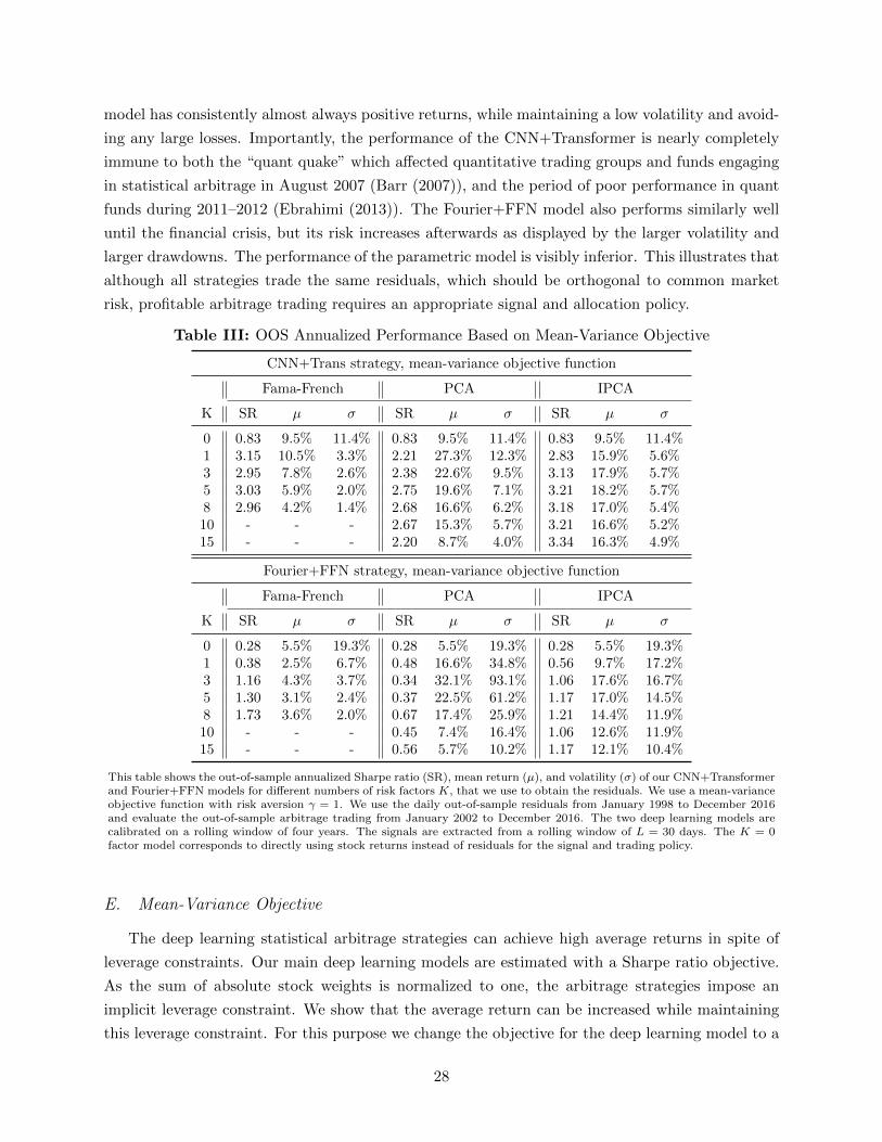
model has consistently almost always positive returns, while maintaining a low volatility and avoid-

ing any large losses. Importantly, the performance of the CNN+Transformer is nearly completely

immune to both the “quant quake” which affected quantitative trading groups and funds engaging

in statistical arbitrage in August 2007 (Barr (2007)), and the period of poor performance in quant

funds during 2011–2012 (Ebrahimi (2013)). The Fourier+FFN model also performs similarly well

until the financial crisis, but its risk increases afterwards as displayed by the larger volatility and

larger drawdowns. The performance of the parametric model is visibly inferior. This illustrates that

although all strategies trade the same residuals, which should be orthogonal to common market

risk, profitable arbitrage trading requires an appropriate signal and allocation policy.

Table III: OOS Annualized Performance Based on Mean-Variance Objective

CNN+Trans strategy, mean-variance objective function

Fama-French PCA IPCA

K SR µ σ SR µ σ SR µ σ

0 0.83 9.5% 11.4% 0.83 9.5% 11.4% 0.83 9.5% 11.4%1 3.15 10.5% 3.3% 2.21 27.3% 12.3% 2.83 15.9% 5.6%3 2.95 7.8% 2.6% 2.38 22.6% 9.5% 3.13 17.9% 5.7%5 3.03 5.9% 2.0% 2.75 19.6% 7.1% 3.21 18.2% 5.7%8 2.96 4.2% 1.4% 2.68 16.6% 6.2% 3.18 17.0% 5.4%10 - - - 2.67 15.3% 5.7% 3.21 16.6% 5.2%15 - - - 2.20 8.7% 4.0% 3.34 16.3% 4.9%

Fourier+FFN strategy, mean-variance objective function

Fama-French PCA IPCA

K SR µ σ SR µ σ SR µ σ

0 0.28 5.5% 19.3% 0.28 5.5% 19.3% 0.28 5.5% 19.3%1 0.38 2.5% 6.7% 0.48 16.6% 34.8% 0.56 9.7% 17.2%3 1.16 4.3% 3.7% 0.34 32.1% 93.1% 1.06 17.6% 16.7%5 1.30 3.1% 2.4% 0.37 22.5% 61.2% 1.17 17.0% 14.5%8 1.73 3.6% 2.0% 0.67 17.4% 25.9% 1.21 14.4% 11.9%10 - - - 0.45 7.4% 16.4% 1.06 12.6% 11.9%15 - - - 0.56 5.7% 10.2% 1.17 12.1% 10.4%

This table shows the out-of-sample annualized Sharpe ratio (SR), mean return (µ), and volatility (σ) of our CNN+Transformerand Fourier+FFN models for different numbers of risk factors K, that we use to obtain the residuals. We use a mean-varianceobjective function with risk aversion γ = 1. We use the daily out-of-sample residuals from January 1998 to December 2016and evaluate the out-of-sample arbitrage trading from January 2002 to December 2016. The two deep learning models arecalibrated on a rolling window of four years. The signals are extracted from a rolling window of L = 30 days. The K = 0factor model corresponds to directly using stock returns instead of residuals for the signal and trading policy.

E. Mean-Variance Objective

The deep learning statistical arbitrage strategies can achieve high average returns in spite of

leverage constraints. Our main deep learning models are estimated with a Sharpe ratio objective.

As the sum of absolute stock weights is normalized to one, the arbitrage strategies impose an

implicit leverage constraint. We show that the average return can be increased while maintaining

this leverage constraint. For this purpose we change the objective for the deep learning model to a

28

mean-variance objective. In order to illustrate the effect of the different objective function, we set

the risk aversion parameter to γ = 1.

Table IV: Significance of Arbitrage Alphas based on Mean-Variance Objective

CNN+Trans model

Fama-French PCA IPCA

K α tα R2 µ tµ α tα R2 µ tµ α tα R2 µ tµ

0 5.8% 2.2∗ 19.6% 9.5% 3.2∗∗ 5.8% 2.2∗ 19.6% 9.5% 3.2∗∗ 5.8% 2.2∗ 19.6% 9.5% 3.2∗∗

1 9.9% 12∗∗∗ 7.1% 10.5% 12∗∗∗ 26.3% 8.3∗∗∗ 1.6% 27.3% 8.6∗∗∗ 14.0% 11∗∗∗ 23.5% 15.9% 11∗∗∗

3 7.5% 11∗∗∗ 5.3% 7.8% 11∗∗∗ 22.1% 9.1∗∗∗ 2.2% 22.6% 9.2∗∗∗ 16.6% 12∗∗∗ 17.6% 17.9% 12∗∗∗

5 5.7% 11∗∗∗ 5.3% 5.9% 12∗∗∗ 19.0% 10∗∗∗ 3.2% 19.6% 11∗∗∗ 16.7% 12∗∗∗ 16.0% 18.2% 12∗∗∗

8 4.4% 9.8∗∗∗ 3.6% 4.6% 10∗∗∗ 16.3% 10∗∗∗ 1.6% 16.6% 10∗∗∗ 15.5% 12∗∗∗ 18.3% 17.0% 12∗∗∗

10 - - - - - 14.8% 10∗∗∗ 1.7% 15.3% 10∗∗∗ 15.2% 13∗∗∗ 20.6% 16.6% 12∗∗∗

15 - - - - - 8.5% 8.4∗∗∗ 0.9% 8.7% 8.5∗∗∗ 14.8% 13∗∗∗ 21.6% 16.3% 13∗∗∗

Fourier+FFN model

Fama-French PCA IPCA

K α tα R2 µ tµ α tα R2 µ tµ α tα R2 µ tµ

0 3.2% 0.7 8.4% 5.5% 1.1 3.2% 0.7 8.4% 5.5% 1.1 3.2% 0.7 8.4% 5.5% 1.11 2.8% 1.6 1.8% 2.5% 1.5 15.4% 1.7 1.3% 16.6% 1.9 7.9% 1.8 2.6% 9.7% 2.2∗

3 4.1% 4.4∗∗∗ 3.4% 4.3% 4.5∗∗∗ 30.3% 1.3 0.1% 32.1% 1.3 17.4% 4.1∗∗∗ 1.9% 17.6% 4.1∗∗∗

5 2.9% 4.8∗∗∗ 3.1% 3.1% 5.0∗∗∗ 21.0% 1.3 0.1% 22.5% 1.4 15.9% 4.3∗∗∗ 2.6% 17.0% 4.5∗∗∗

8 3.5% 6.8∗∗∗ 2.3% 3.6% 7.0∗∗∗ 17.4% 2.6∗∗ 0.3% 17.2% 2.6∗∗ 12.9% 4.3∗∗∗ 4.4% 14.4% 4.7∗∗∗

10 - - - - - 7.1% 1.7 0.3% 7.4% 1.8 11.7% 3.9∗∗∗ 3.5% 12.6% 4.1∗∗∗

15 - - - - - 5.5% 2.1∗ 0.1% 5.7% 2.2∗ 11.3% 4.3∗∗∗ 4.0% 12.1% 4.5∗∗∗

This table shows the out-of-sample pricing errors α of the arbitrage strategies relative of the Fama-French 8 factor model andtheir mean returns µ for the different arbitrage models and different number of factors K that we use to obtain the residuals.We use a mean-variance objective function with risk aversion γ = 1. We run a time-series regression of the out-of-samplereturns of the arbitrage strategies on the 8-factor model (Fama-French 5 factors + momentum + short-term reversal + long-term reversal) and report the annualized α, accompanying t-statistic value tα, and the R2 of the regression. In addition, wereport the annualized mean return µ along with its accompanying t-statistic tµ. The hypothesis test are two-sided and starsindicate p-values of 5% (∗), 1% (∗∗), and 0.1% (∗∗∗). All results use the out-of-sample daily returns from January 2002 toDecember 2016.

Tables III and IV collect the results for the Sharpe ratio, mean, volatility and significance tests.

As expected the Sharpe ratios are slightly lower compared to the corresponding model with Sharpe

ratio objective, but the mean returns are substantially increased. The CNN+Transformer model

achieves average annual returns around 20% with PCA and IPCA residuals while the volatility

is only around half as large as the one of a market portfolio. The mean returns are statistically

highly significant and not spanned by conventional risk factors or a price trend risk premium.

The Fourier+FFN model can also obtain high average returns, but those come at the cost of a

substantial volatility. Overall, we confirm that the more flexible signal extraction function of the

CNN+Transformer is crucial for the superior performance.

F. Unconditional Residual Means

The unconditional average of residuals is not a profitable strategy and does not provide infor-

mation about the potential arbitrage profitability contained in the residuals. A natural question

to ask is if the residuals themselves have a risk premium component and if trading an equally

weighted portfolio of residuals could be profitable. Table V shows the performance of this simple

29

strategy. If we do not project out any factors (K = 0), this strategy essentially trades an equally

weighted market portfolio. Table VI reports the test statistics relative to the Fama-French 8 factor

model, which completely subsumes the market risk premium. Once we regress out at least 3 fac-

tors, the equally weighted residuals have a mean return of around 1% or lower. The low volatility

confirms that the residuals are only weakly cross-sectionally dependent and are largely diversified

away. The moderately large Sharpe ratios for PCA residuals is a consequence of the near zero

volatility. Scaling up the mean returns to a meaningful magnitude would potentially require an

unreasonable amount of leverage. Overall, we confirm that residuals need to be combined with

a signal and trading policy that takes advantage of the time series patterns in order to achieve a

profitable strategy.

Table V: OOS Annualized Performance of Unconditional Average Residuals

Equally Weighted Residuals

Fama-French PCA IPCA

K SR µ σ SR µ σ SR µ σ

0 0.52 11.2% 21.4% 0.52 11.2% 21.4% 0.52 11.2% 21.4%

1 0.39 1.9% 4.8% -0.23 -0.4% 1.5% 0.76 3.2% 4.2%

3 0.18 0.7% 3.7% 0.34 0.3% 0.9% 0.76 2.0% 2.7%

5 0.22 0.8% 3.5% 0.93 0.7% 0.7% 0.63 1.4% 2.3%

8 -0.17 -0.5% 2.9% 1.04 0.6% 0.5% 0.66 1.4% 2.2%

10 - - - 0.90 0.4% 0.5% 0.65 1.3% 2.1%

15 - - - 1.08 0.4% 0.4% 0.62 1.3% 2.0%

This table shows the out-of-sample annualized Sharpe ratio (SR), mean return (µ), and volatility (σ) of equally weightedresiduals. We evaluate the out-of-sample arbitrage trading from January 2002 to December 2016. The K = 0 factor modelcorresponds to directly using stock returns instead of residuals for the signal and trading policy.

IPCA factors are close to uncorrelated with conventional risk factors. The R2 values in Table

VI are as expected for the Fama-French factors and, not surprisingly, after regressing out all of

those factors, the cross-sectional average of the residuals is essentially orthogonal to those factors.

The PCA residuals show a very similar behavior. However, the conditional IPCA model leaves a

component in the residuals that it is highly correlated with conventional risk factors. In this sense,

the IPCA factors extract a factor model that is quite different from the Fama-French factors.

Importantly, unconditional means and alphas of asset pricing residuals are a poor measure of

arbitrage opportunities. The mean and alphas of residuals that are optimally traded based on their

time series patterns have mean returns that can be larger by a factor of 50. This implies more

generally, that the unconditional perspective of evaluating asset pricing models could potentially

overstate the efficiency of markets and the pricing ability of asset pricing models.

30

Table VI: Significance of Arbitrage Alphas Based on Unconditional Average Residuals

Equally Weighted Residuals

Fama-French PCA IPCA

K α tα R2 µ tµ α tα R2 µ tµ α tα R2 µ tµ

0 1.4% 1.4 97.0% 11.2% 2.0∗ 1.4% 1.4 97.0% 11.2% 2.0∗ 1.4% 1.4 97.0% 11.2% 2.0∗

1 0.4% 0.4 36.6% 1.9% 1.5 0.0% 0.0 25.8% -0.4% -0.9 0.4% 1.1 85.0% 3.2% 2.9∗∗

3 0.4% 0.4 9.6% 0.7% 0.7 0.4% 1.9 13.1% 0.3% 1.3 0.9% 3.3∗∗ 84.1% 2.0% 2.9∗∗

5 0.2% 0.2 7.0% 0.8% 0.9 0.7% 4.2∗∗∗ 5.9% 0.7% 3.6∗∗∗ 0.4% 2.0∗ 89.4% 1.4% 2.4∗

8 -0.6% -0.8 0.7% -0.5% -0.7 0.6% 4.5∗∗∗ 4.1% 0.6% 4.0∗∗∗ 0.4% 2.1∗ 89.3% 1.4% 2.5∗

10 - - - - - 0.5% 3.8∗∗∗ 3.0% 0.4% 3.5∗∗∗ 0.3% 1.9 89.4% 1.3% 2.5∗

15 - - - - - 0.4% 4.3∗∗∗ 2.0% 0.4% 4.2∗∗∗ 0.3% 1.6 89.0% 1.3% 2.4∗

This table shows the out-of-sample pricing errors α of cross-sectionally equally weighted residuals relative of the Fama-French8 factor model and their mean returns µ for the different arbitrage models and different number of factors K that we useto obtain the residuals. We run a time-series regression of the out-of-sample returns of the arbitrage strategies on the 8-factor model (Fama-French 5 factors + momentum + short-term reversal + long-term reversal) and report the annualized α,accompanying t-statistic value tα, and the R2 of the regression. In addition, we report the annualized mean return µ alongwith its accompanying t-statistic tµ. The hypothesis test are two-sided and stars indicate p-values of 5% (∗), 1% (∗∗), and0.1% (∗∗∗). All results use the out-of-sample daily returns from January 2002 to December 2016.

G. Importance of Time-Series Signal

How important is the flexibility in the signal extraction function relative to the allocation

function? So far, we have considered a rigid parametric model for the signal and allocation function

and a flexible allocation function but either a pre-specified time-series filter or a data-driven flexible

filter. In A.VII in Appendix we also report the results for two additional model variations, which

serve as ablation tests emphasizing the central importance of applying a time-series model to extract

a signal extraction function from the data.

The first model, OU+FFN, uses the same 4-dimensional OU signal as the OU+Threshold

policy, but replaces the threshold allocation function with an FFN allocation function. This FFN

allocation function has the same architecture as that of the Fourier+FFN policy, except the input

is 4-dimensional instead of 30-dimensional. The results show that even despite using a very flexible

allocation function, the results are similar or even worse than the simple parametric thresholding

rule. This points to the weakness of the OU signal representation: although the allocation function

is a powerful universal approximator, it cannot accomplish much with an information-poor input. If

the optimal allocation function given the simple OU signal is well approximated by the parametric

thresholding rule, then the nonparametric FFN offers too much flexibility without comparable

efficiency, which leads to a noisier estimate of a simple function and hence worse out-of-sample

performance.

The second model does not extract a time-series signal from the residuals, but uses the residuals

themselves as signal to a flexible FFN allocation function. As the allocation function uses the same

type of network as for the CNN+Transformer, Fourier+FFN or OU+FFN, this setup directly

assesses the relevance of using a time-series model for the signal. The FFN model also performs

worse than the deep learning models that apply a time-series filter to the residuals. This is a good

example to emphasize the importance of a time-series model. While FFNs are flexible in learning

31

low dimensional functional relationships, they are limited in learning a complex dependency model

if the training data is limited. For example, the FFN is not sufficiently efficient to learn an FFT-

like transformation and hence has a substantially worse performance on the original time-series

compared to frequency-transformed time-series.

In summary, the flexible data-driven signal extraction function of the CNN+Transformer model

seems to be the critical element for statistical arbitrage. A flexible allocation function is not

sufficient to compensate for an uninformative signal.

H. Dependency between Arbitrage Strategies

The trading strategies for different factor models are only weakly correlated. In Table A.VI,

we report the correlations of the returns of our CNN+Transformer strategies across factor models

with 3, 5, and 10 factors, based on the Sharpe ratio objective function strategy.13 Notably, the

correlations between strategies from different factor model families range from roughly 0.2 to 0.45,

indicating that strategies for different factor model families can be used as part of a diversification

strategy. While the performance of the arbitrage trading for the residuals obtained with different

families of factor models is comparable, the factors themselves are different. Hence, even if the

arbitrage signal and allocation functions are similar, the resulting strategies can be weakly corre-

lated. The within-family correlations range from 0.4 to 0.85, indicating that the residuals from the

same class of factor model capture similar patterns.

I. Stability over Time

Our results are robust to length of the local window to extract the trading signal. We re-

estimate the CNN+Transformer model on an extended rolling lookback window of L = 60 days,

while keeping the rest of the model structure the same. Tables VII and VIII show that the results

are robust to the choice of lookback window. Extending the local window to 60 trading days, which

is close to three months, leads to essentially the same performance as using only the most recent

L = 30 trading days to infer the signal. This is further evidence that the arbitrage signal is different

from conventional momentum or reversal strategies that incorporate information from longer time

periods. As the signal can be inferred from the most recent past, it implies that either the arbitrage

signal depends only on the most recent days or that those days are sufficient to infer the relevant

time-series structure. In the next section, we provide evidence that the arbitrage trading signals

put strong emphasis on most recent two weeks before the trading.

A constant-in-time signal and allocation function captures a large fraction of the arbitrage infor-

mation. We re-estimate the CNN+Transformer model with a constant model instead of the rolling

window calibration. Our main models are estimated on a rolling window of four years, which allows

the models to adopt to changing economic conditions. Here we use either the first Ttrain = 4 years

(1,000 trading days) or Ttrain = 8 years (2,000 trading days) to estimate the signal and allocation

13The correlations for the mean-variance objective function are similar.

32

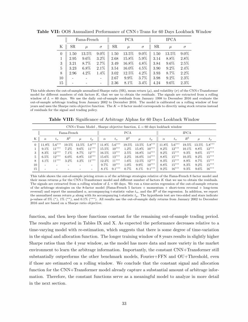
Table VII: OOS Annualized Performance of CNN+Trans for 60 Days Lookback Window

Fama-French PCA IPCA

K SR µ σ SR µ σ SR µ σ

0 1.50 13.5% 9.0% 1.50 13.5% 9.0% 1.50 13.5% 9.0%1 2.95 9.6% 3.2% 2.68 15.8% 5.9% 3.14 8.8% 2.8%3 3.21 8.7% 2.7% 3.49 16.8% 4.8% 3.84 9.6% 2.5%5 3.23 6.8% 2.1% 3.54 16.0% 4.5% 3.90 9.2% 2.4%8 2.96 4.2% 1.4% 3.02 12.5% 4.2% 3.93 8.7% 2.2%10 - - - 2.67 9.9% 3.7% 3.98 9.2% 2.3%15 - - - 2.36 8.1% 3.4% 4.24 9.6% 2.3%

This table shows the out-of-sample annualized Sharpe ratio (SR), mean return (µ), and volatility (σ) of the CNN+Transformermodel for different numbers of risk factors K, that we use to obtain the residuals. The signals are extracted from a rollingwindow of L = 60 days. We use the daily out-of-sample residuals from January 1998 to December 2016 and evaluate theout-of-sample arbitrage trading from January 2002 to December 2016. The model is calibrated on a rolling window of fouryears and uses the Sharpe ratio objective function. The K = 0 factor model corresponds to directly using stock returns insteadof residuals for the signal and trading policy.

Table VIII: Significance of Arbitrage Alphas for 60 Days Lookback Window

CNN+Trans Model , Sharpe objective function, L = 60 days lookback window

Fama-French PCA IPCA

K α tα R2 µ tµ α tα R2 µ tµ α tα R2 µ tµ

0 11.8% 5.6∗∗∗ 19.5% 13.5% 5.8∗∗∗ 11.8% 5.6∗∗∗ 19.5% 13.5% 5.8∗∗∗ 11.8% 5.6∗∗∗ 19.5% 13.5% 5.8∗∗∗

1 9.1% 11∗∗∗ 7.2% 9.6% 11∗∗∗ 15.5% 10∗∗∗ 1.2% 15.8% 10∗∗∗ 8.2% 12∗∗∗ 10.1% 8.8% 12∗∗∗

3 8.3% 12∗∗∗ 7.1% 8.7% 12∗∗∗ 16.5% 13∗∗∗ 2.5% 16.8% 14∗∗∗ 9.2% 15∗∗∗ 9.3% 9.6% 15∗∗∗

5 6.5% 12∗∗∗ 6.0% 6.8% 13∗∗∗ 15.6% 13∗∗∗ 2.2% 16.0% 14∗∗∗ 8.8% 15∗∗∗ 10.3% 9.2% 15∗∗∗

8 4.1% 11∗∗∗ 3.2% 4.2% 11∗∗∗ 12.2% 11∗∗∗ 1.6% 12.5% 12∗∗∗ 8.3% 15∗∗∗ 8.9% 8.7% 15∗∗∗

10 - - - - - 9.7% 10∗∗∗ 1.0% 9.9% 10∗∗∗ 8.8% 15∗∗∗ 8.3% 9.2% 15∗∗∗

15 - - - - - 8.1% 9.1∗∗∗ 0.7% 8.1% 9.1∗∗∗ 9.2% 16∗∗∗ 9.3% 9.6% 16∗∗∗

This table shows the out-of-sample pricing errors α of the arbitrage strategies relative of the Fama-French 8 factor model andtheir mean returns µ for the CNN+Transformer model and different number of factors K that we use to obtain the residuals.The signals are extracted from a rolling window of L = 60 days. We run a time-series regression of the out-of-sample returnsof the arbitrage strategies on the 8-factor model (Fama-French 5 factors + momentum + short-term reversal + long-termreversal) and report the annualized α, accompanying t-statistic value tα, and the R2 of the regression. In addition, we reportthe annualized mean return µ along with its accompanying t-statistic tµ. The hypothesis test are two-sided and stars indicatep-values of 5% (∗), 1% (∗∗), and 0.1% (∗∗∗). All results use the out-of-sample daily returns from January 2002 to December2016 and are based on a Sharpe ratio objective.

function, and then keep those functions constant for the remaining out-of-sample trading period.

The results are reported in Tables IX and X. As expected the performance decreases relative to a

time-varying model with re-estimation, which suggests that there is some degree of time-variation

in the signal and allocation function. The longer training window of 8 years results in slightly higher

Sharpe ratios than the 4 year window, as the model has more data and more variety in the market

environment to learn the arbitrage information. Importantly, the constant CNN+Transformer still

substantially outperforms the other benchmark models, Fourier+FFN and OU+Threshold, even

if those are estimated on a rolling window. We conclude that the constant signal and allocation

function for the CNN+Transformer model already capture a substantial amount of arbitrage infor-

mation. Therefore, the constant functions serve as a meaningful model to analyze in more detail

in the next section.

33

Table IX: OOS Annualized Performance of CNN+Trans for Constant Model

Ttrain = 4 years

Fama-French PCA IPCA

K SR µ σ SR µ σ SR µ σ

0 1.10 8.5% 7.8% 1.10 8.5% 7.8% 1.10 8.5% 7.8%1 1.90 4.5% 2.3% 0.66 5.2% 7.9% 0.94 3.1% 3.3%3 1.60 3.6% 2.2% 1.65 8.7% 5.3% 1.82 5.3% 2.9%5 1.81 3.0% 1.7% 1.93 9.8% 5.1% 2.09 5.4% 2.6%8 1.70 2.5% 1.5% 2.04 9.6% 4.7% 1.89 5.0% 2.6%10 - - - 2.06 9.1% 4.4% 1.77 4.7% 2.7%15 - - - 1.82 7.0% 3.9% 2.09 5.5% 2.7%

Ttrain = 8 years

Fama-French PCA IPCA

K SR µ σ SR µ σ SR µ σ

0 1.33 12.0% 9.0% 1.33 12.0% 9.0% 1.33 12.0% 9.0%1 2.06 5.0% 2.4% 1.81 15.2% 8.4% 2.02 8.5% 4.2%3 2.46 5.3% 2.2% 2.04 13.1% 6.4% 2.47 7.5% 3.0%5 1.82 3.2% 1.8% 1.91 11.9% 6.2% 2.64 7.6% 2.9%8 1.48 2.5% 1.7% 1.89 10.8% 5.7% 2.71 8.3% 3.1%10 - - - 1.82 10.0% 5.5% 2.68 8.2% 3.1%15 - - - 1.38 6.2% 4.5% 2.70 7.8% 2.9%

This table shows the out-of-sample annualized Sharpe ratio (SR), mean return (µ), and volatility (σ) of the CNN+Transformermodel for different numbers of risk factors K. We estimate the model on only once on the first Ttrain days and keep it constanton the remaining test set. We use the daily out-of-sample residuals from January 1998 to December 2016 and evaluate theout-of-sample arbitrage trading from January 1998 +Ttrain to December 2016. The signals are extracted from a rolling windowof L = 30 days and we use the Sharpe ratio objective function.

J. Estimated Structure

What are the patterns that our CNN+Transformer model can learn and exploit? In order

to answer this question, we analyze the different building blocks of our benchmark model and

show their structure on representative and informative residuals inputs. Our goal is to ascertain,

characterize, and explain the role that the convolutional features and attention heads play in the

determination of the final allocation weight and recognition of salient time series patterns. The

benchmark model for this section is the CNN+Transformer based on IPCA 5-factor residuals and

a Sharpe ratio objective. The model is calibrated on the first 8 years of data and kept constant,

which allows us to study the signal and allocation function.

As an illustrative example, Figure 7 shows the allocation and return on representative residuals.

The left subplot displays an out-of-sample time-series of cumulative returns of a randomly selected

residual and its value in the allocation function. We normalize the allocation weight to have an

absolute value of one, that is, for this illustrative example we only trade this particular residual.

The right subplots depicts the payoff of trading the specific residual with the displayed allocation

function. The first residual shows mean-reversion patterns, which are successfully detected and

exploited by the function wε|CNN+Trans. The second residual has a downward trend, which is

34

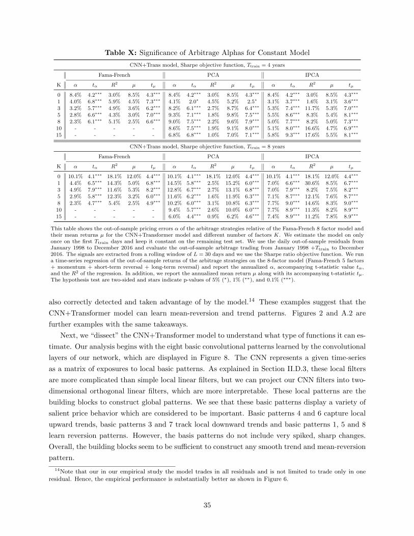
Table X: Significance of Arbitrage Alphas for Constant Model

CNN+Trans model, Sharpe objective function, Ttrain = 4 years

Fama-French PCA IPCA

K α tα R2 µ tµ α tα R2 µ tµ α tα R2 µ tµ

0 8.4% 4.2∗∗∗ 3.0% 8.5% 4.3∗∗∗ 8.4% 4.2∗∗∗ 3.0% 8.5% 4.3∗∗∗ 8.4% 4.2∗∗∗ 3.0% 8.5% 4.3∗∗∗

1 4.0% 6.8∗∗∗ 5.9% 4.5% 7.3∗∗∗ 4.1% 2.0∗ 4.5% 5.2% 2.5∗ 3.1% 3.7∗∗∗ 1.6% 3.1% 3.6∗∗∗

3 3.2% 5.7∗∗∗ 4.9% 3.6% 6.2∗∗∗ 8.2% 6.1∗∗∗ 2.7% 8.7% 6.4∗∗∗ 5.3% 7.4∗∗∗ 11.7% 5.3% 7.0∗∗∗

5 2.8% 6.6∗∗∗ 4.3% 3.0% 7.0∗∗∗ 9.3% 7.1∗∗∗ 1.8% 9.8% 7.5∗∗∗ 5.5% 8.6∗∗∗ 8.3% 5.4% 8.1∗∗∗

8 2.3% 6.1∗∗∗ 5.1% 2.5% 6.6∗∗∗ 9.0% 7.5∗∗∗ 2.2% 9.6% 7.9∗∗∗ 5.0% 7.7∗∗∗ 8.2% 5.0% 7.3∗∗∗

10 - - - - - 8.6% 7.5∗∗∗ 1.9% 9.1% 8.0∗∗∗ 5.1% 8.0∗∗∗ 16.6% 4.7% 6.9∗∗∗

15 - - - - - 6.8% 6.8∗∗∗ 1.0% 7.0% 7.1∗∗∗ 5.8% 9.3∗∗∗ 17.6% 5.5% 8.1∗∗∗

CNN+Trans model, Sharpe objective function, Ttrain = 8 years

Fama-French PCA IPCA

K α tα R2 µ tµ α tα R2 µ tµ α tα R2 µ tµ

0 10.1% 4.1∗∗∗ 18.1% 12.0% 4.4∗∗∗ 10.1% 4.1∗∗∗ 18.1% 12.0% 4.4∗∗∗ 10.1% 4.1∗∗∗ 18.1% 12.0% 4.4∗∗∗

1 4.4% 6.5∗∗∗ 14.3% 5.0% 6.8∗∗∗ 14.5% 5.8∗∗∗ 2.5% 15.2% 6.0∗∗∗ 7.0% 6.6∗∗∗ 30.6% 8.5% 6.7∗∗∗

3 4.9% 7.9∗∗∗ 11.6% 5.3% 8.2∗∗∗ 12.8% 6.7∗∗∗ 2.7% 13.1% 6.8∗∗∗ 7.0% 7.9∗∗∗ 8.2% 7.5% 8.2∗∗∗

5 2.9% 5.8∗∗∗ 12.3% 3.2% 6.0∗∗∗ 11.6% 6.2∗∗∗ 1.6% 11.9% 6.3∗∗∗ 7.1% 8.7∗∗∗ 12.1% 7.6% 8.7∗∗∗

8 2.3% 4.7∗∗∗ 5.4% 2.5% 4.9∗∗∗ 10.2% 6.0∗∗∗ 3.1% 10.8% 6.3∗∗∗ 7.7% 9.0∗∗∗ 14.6% 8.3% 9.0∗∗∗

10 - - - - - 9.4% 5.7∗∗∗ 2.6% 10.0% 6.0∗∗∗ 7.7% 8.9∗∗∗ 11.3% 8.2% 8.9∗∗∗

15 - - - - - 6.0% 4.4∗∗∗ 0.9% 6.2% 4.6∗∗∗ 7.4% 8.9∗∗∗ 11.2% 7.8% 8.9∗∗∗

This table shows the out-of-sample pricing errors α of the arbitrage strategies relative of the Fama-French 8 factor model andtheir mean returns µ for the CNN+Transformer model and different number of factors K. We estimate the model on onlyonce on the first Ttrain days and keep it constant on the remaining test set. We use the daily out-of-sample residuals fromJanuary 1998 to December 2016 and evaluate the out-of-sample arbitrage trading from January 1998 +Ttrain to December2016. The signals are extracted from a rolling window of L = 30 days and we use the Sharpe ratio objective function. We runa time-series regression of the out-of-sample returns of the arbitrage strategies on the 8-factor model (Fama-French 5 factors+ momentum + short-term reversal + long-term reversal) and report the annualized α, accompanying t-statistic value tα,and the R2 of the regression. In addition, we report the annualized mean return µ along with its accompanying t-statistic tµ.The hypothesis test are two-sided and stars indicate p-values of 5% (∗), 1% (∗∗), and 0.1% (∗∗∗).

also correctly detected and taken advantage of by the model.14 These examples suggest that the

CNN+Transformer model can learn mean-reversion and trend patterns. Figures 2 and A.2 are

further examples with the same takeaways.

Next, we “dissect” the CNN+Transformer model to understand what type of functions it can es-

timate. Our analysis begins with the eight basic convolutional patterns learned by the convolutional

layers of our network, which are displayed in Figure 8. The CNN represents a given time-series

as a matrix of exposures to local basic patterns. As explained in Section II.D.3, these local filters

are more complicated than simple local linear filters, but we can project our CNN filters into two-

dimensional orthogonal linear filters, which are more interpretable. These local patterns are the

building blocks to construct global patterns. We see that these basic patterns display a variety of

salient price behavior which are considered to be important. Basic patterns 4 and 6 capture local

upward trends, basic patterns 3 and 7 track local downward trends and basic patterns 1, 5 and 8

learn reversion patterns. However, the basis patterns do not include very spiked, sharp changes.

Overall, the building blocks seem to be sufficient to construct any smooth trend and mean-reversion

pattern.

14Note that our in our empirical study the model trades in all residuals and is not limited to trade only in oneresidual. Hence, the empirical performance is substantially better as shown in Figure 6.

35

Figure 7: Examples of Allocation and Returns of CNN+Transformer Strategy

These plots display representative examples of the CNN+Transformer out-of-sample arbitrage trading on a sample of residualsfrom the IPCA 5-factor model. The left subplots show the normalized cumulative returns of the residuals and the normalizedallocation weight, which the specific residual has in the trading strategy. The right subplots illustrates the payoff of tradingthe specific residual with the displayed allocation function. The model is calibrated on the first 8 years of data and keptconstant.

We can understand the global patterns learned by the transformer by studying the attention

function. The attention functions αi(., .) of each attention head i = 1, ...,H = 4 capture the

dependencies between the local patterns. Our arbitrage signal can be interpreted as “loadings” to

these “attention factors”. We use the same H attention functions for all residuals, but in order to

visualize them, we evaluate them for a given residual time-series, which yield the attention weights

per head:

αi,l,j = αi (xl, xj) for i = 1, ...,H.

As our signal only depends on the final cumulative return projection hprojL , the attention weights

αi,L,j for i = 1, ..,H and j = 1, ..., L contain all the “global factor” information. Hence, we will

plot the H × L dimensional attention weights of the attention heads to understand which global

patterns are activated by specific time-series.

Figure 9 plots the attention head weights for simulated sinusoidal residual input time-series.

Note that the attention head weights discover the sinusoidal pattern although the model was es-

timated on the empirical data and not specifically trained for this simulated input. The different

attention heads capture different patterns. The fourth attention head displayed in red has the

36

Figure 8: Local Basic Patterns of Benchmark Model

(a) Basic pattern 1 (b) Basic pattern 2 (c) Basic pattern 3 (d) Basic pattern 4

(e) Basic pattern 5 (f) Basic pattern 6 (g) Basic pattern 7 (h) Basic pattern 8

These figures show the D = 8 local filters of the CNN estimated for the benchmark model in our empirical analysis. These areprojections of our higher dimensional nonlinear filter from a 2-layer CNN into two-dimensional linear filters. These buildingblocks are labeled “basic patterns”. The benchmark model is the CNN+Transformer model based on IPCA 5-factor residuals.We estimate the model on only once on the first Ttrain=8 years based on the Sharpe ratio objective.

strongest activation and capture high-frequency mean reversion patterns. These attention head

weights are positive for negative realizations. We will label these fourth attention head weights a

“negative reversal” pattern. The third attention head weights depicted by the green curve co-move

with the mean-reversion patterns of the original time-series, that is they are positive for high values,

but seem to be only activated if this positive “hilltop” appears at the beginning of the time-series.

If the mean-reversion cycle achieves its positive values at the end, the third attention head is not

activated. We will label these third attention head weights the “early reversal” pattern. The first

attention head in blue seems to be a “dampened” version of the fourth red attention head. Figure

A.3 in the Appendix shows additional simulated input time-series that confirm this interpretation.

In summary, the different attention head weights can be assigned to specific global patterns.

In Figure 10, we plot the different components of the CNN+Transformer model evaluated on a

randomly selected, representative 30-day empirical residual. The cumulative residual in subfigure

(a) is the input to the CNN. This L = 30 dimensional vector is represented by the CNN in terms

of its “exposure” to local basic pattern. The subfigures (d)–(k) show this D × L dimensional

representation, which is the output of the CNN. As we have D = 8 local filters, we obtain eight

time-series that display the activation to each filter. For example, basic pattern 1 is associated

with a “reversal kink” in subfigure 8(a) and hence has the strongest activation to this basic pattern

on day 28, when the residual has a downward spike. This D × L matrix of exposures to local

patterns is the input to the transformer. The attention head weights in subfigure (b) connect

the local patterns to a global pattern. The fourth attention head weight in red has its highest

values during the “bottom” of the residual movements, confirming our previous intuition that this

37

Figure 9: Example Attention Weights for Sinusoidal Residual Inputs

(a) Input residual and attention head weights for xl = sin(2π l

30

)

(b) Input residual and attention head weights for for xl = sin(2π l+15

30

)These plots show the attention head weights of the CNN+Transformer benchmark model for simulated sinusoidal residualinput time series. Both sine functions have a cycle of 30 days and the second is shifted by 15 days. The right subplotshows the attention weights for the H = 4 attention heads for the specific residuals. The empirical benchmark model is theCNN+Transformer model based on IPCA 5-factor residuals. We estimate the model on only once on the first Ttrain=8 yearsbased on the Sharpe ratio objective.

attention head activates during bad times. The third attention head weight in green spikes during

the “top” at the beginning of the residual time-series, which is in line with our interpretation as an

early reversal pattern. The first attention head in blue is a dampened version of the red attention

head. The average over the four attention head weights depicted in subfigure (c) suggests that the

heads attend on average more closely to the latter half of the time series.

In Figure 11 we generalize the analysis of Figure 10 to study the model structure of the bench-

mark model over time. While Figure 10 represents a “snapshot” for one point in time, we now

display the allocation weights and attention head weights of a single representative residual for

different times. Subfigure 11(a) shows the cumulative residual time-series. For a specific point in

time we use the lagged L = 30 days as an input to obtain the allocation weights and attention head

weights for that time. The out-of-sample allocation weights correctly change the directions to ex-

ploit the patterns in the residual time-series. The attention head weights over time offer additional

insights into the structure of the global patterns. Each vertical slice from window index 1 to window

index 30 displays the normalized attention weights for the time point under the slice. The third

attention head, which was displayed in green in Figures 9 and 10 has the largest values during “up-

patterns” of the residual, for example for 2007, 2010 and 2012. Importantly, the attention weights

focus on the early days within the 30-day window. This confirms our previous interpretation as an

“early reversal” pattern. Attention head four, which was previously represented as a red line, has

38

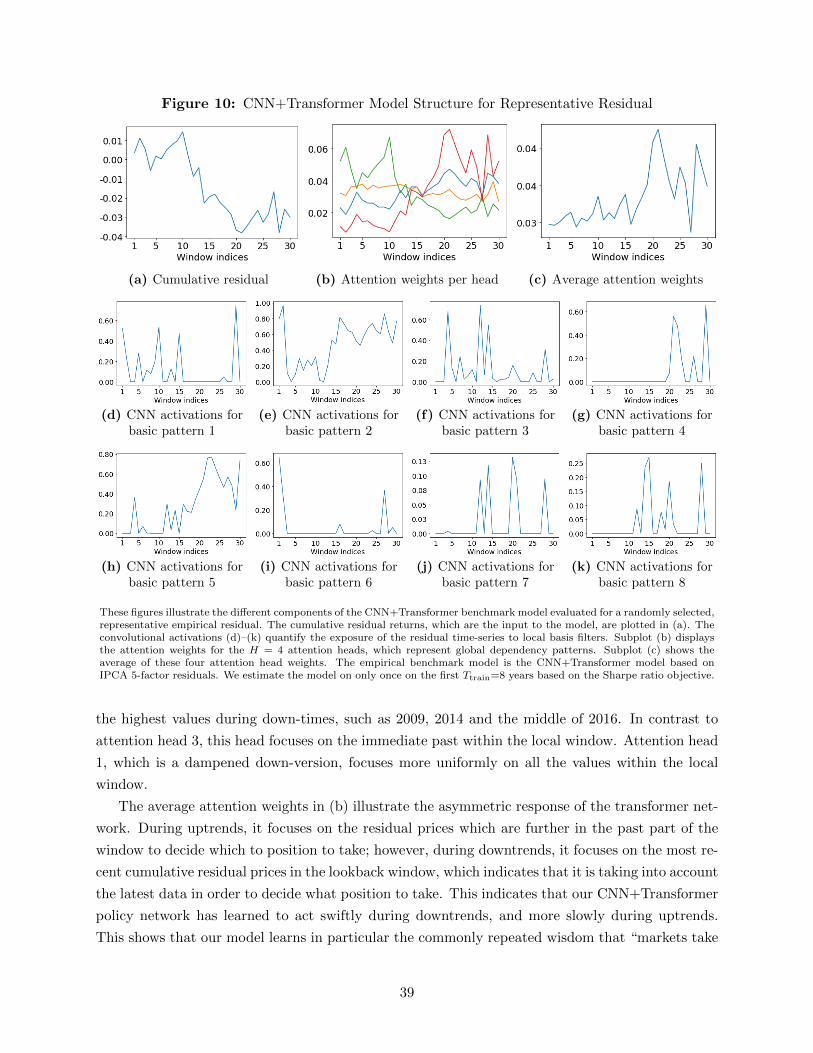
Figure 10: CNN+Transformer Model Structure for Representative Residual

(a) Cumulative residual (b) Attention weights per head (c) Average attention weights

(d) CNN activations forbasic pattern 1

(e) CNN activations forbasic pattern 2

(f) CNN activations forbasic pattern 3

(g) CNN activations forbasic pattern 4

(h) CNN activations forbasic pattern 5

(i) CNN activations forbasic pattern 6

(j) CNN activations forbasic pattern 7

(k) CNN activations forbasic pattern 8

These figures illustrate the different components of the CNN+Transformer benchmark model evaluated for a randomly selected,representative empirical residual. The cumulative residual returns, which are the input to the model, are plotted in (a). Theconvolutional activations (d)–(k) quantify the exposure of the residual time-series to local basis filters. Subplot (b) displaysthe attention weights for the H = 4 attention heads, which represent global dependency patterns. Subplot (c) shows theaverage of these four attention head weights. The empirical benchmark model is the CNN+Transformer model based onIPCA 5-factor residuals. We estimate the model on only once on the first Ttrain=8 years based on the Sharpe ratio objective.

the highest values during down-times, such as 2009, 2014 and the middle of 2016. In contrast to

attention head 3, this head focuses on the immediate past within the local window. Attention head

1, which is a dampened down-version, focuses more uniformly on all the values within the local

window.

The average attention weights in (b) illustrate the asymmetric response of the transformer net-

work. During uptrends, it focuses on the residual prices which are further in the past part of the

window to decide which to position to take; however, during downtrends, it focuses on the most re-

cent cumulative residual prices in the lookback window, which indicates that it is taking into account

the latest data in order to decide what position to take. This indicates that our CNN+Transformer

policy network has learned to act swiftly during downtrends, and more slowly during uptrends.

This shows that our model learns in particular the commonly repeated wisdom that “markets take

39

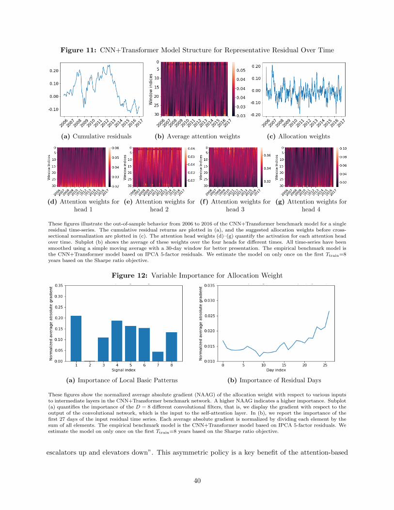
Figure 11: CNN+Transformer Model Structure for Representative Residual Over Time

(a) Cumulative residuals (b) Average attention weights (c) Allocation weights

(d) Attention weights forhead 1

(e) Attention weights forhead 2

(f) Attention weights forhead 3

(g) Attention weights forhead 4

These figures illustrate the out-of-sample behavior from 2006 to 2016 of the CNN+Transformer benchmark model for a singleresidual time-series. The cumulative residual returns are plotted in (a), and the suggested allocation weights before cross-sectional normalization are plotted in (c). The attention head weights (d)–(g) quantify the activation for each attention headover time. Subplot (b) shows the average of these weights over the four heads for different times. All time-series have beensmoothed using a simple moving average with a 30-day window for better presentation. The empirical benchmark model isthe CNN+Transformer model based on IPCA 5-factor residuals. We estimate the model on only once on the first Ttrain=8years based on the Sharpe ratio objective.

Figure 12: Variable Importance for Allocation Weight

(a) Importance of Local Basic Patterns (b) Importance of Residual Days

These figures show the normalized average absolute gradient (NAAG) of the allocation weight with respect to various inputsto intermediate layers in the CNN+Transformer benchmark network. A higher NAAG indicates a higher importance. Subplot(a) quantifies the importance of the D = 8 different convolutional filters, that is, we display the gradient with respect to theoutput of the convolutional network, which is the input to the self-attention layer. In (b), we report the importance of thefirst 27 days of the input residual time series. Each average absolute gradient is normalized by dividing each element by thesum of all elements. The empirical benchmark model is the CNN+Transformer model based on IPCA 5-factor residuals. Weestimate the model on only once on the first Ttrain=8 years based on the Sharpe ratio objective.

escalators up and elevators down”. This asymmetric policy is a key benefit of the attention-based

40

model, which cannot easily be replicated by the parametric Ornstein-Uhlenbeck or fixed basis pat-

tern benchmark models we compare against. The convolutional subnetwork’s patterns provide

translation invariant information about what kind of trend is present within each 3-day subwindow

of the 30-day cumulative residual price lookback window, which allows the transformer subnetwork

to form a stable attention function that results in this unique policy.

Figure 12 sheds further light on which days and patterns are important. The figure shows

the normalized average absolute gradient (NAAG) of the allocation weight with respect to various

inputs to intermediate layers in the CNN+Transformer benchmark network. A higher NAAG

indicates a higher importance. Subplot (a) quantifies the importance of the D = 8 different basic

patterns. We observe that the flat basic pattern 2 has a negligible weight, while basis patterns that

are needed for trend or reversal patterns have high importance. In (b), we report the importance

of the first 27 days of the input residual time series.15 Crucially, all previous days matter, which

emphasizes that the trading allocation depends on the past dynamics. The most recent 14 days

seem to get on average more attention for the trading decisions. However, as indicated in Figure

11, the importance of the days seems to be asymmetric for different global patterns.

K. Market Frictions and Transaction Costs

Our deep learning arbitrage strategies remain profitable in the presence of realistic trading

frictions. In practice, trading costs associated with high turnover or large short-selling positions

can diminish the profitability of arbitrage trading. In order to ensure that our model produces

economically meaningful results, we extend it to the setting in which both transaction costs and

holding costs are accounted for. We do not model market frictions associated with market impact,

as in our empirical analysis we restrict the asset universe to stocks with large market capitalization,

which are especially liquid.

Table XI: OOS Performance of CNN+Trans with Trading Frictions

IPCA factor model

Sharpe ratio Mean-variance

K SR µ σ SR µ σ

0 0.52 8.5% 16.3% 0.22 2.6% 11.9%1 0.85 5.9% 6.9% 0.86 5.5% 6.4%3 1.24 6.6% 5.4% 1.16 6.9% 5.9%5 1.11 5.5% 5.0% 1.02 5.3% 5.3%10 0.98 5.1% 5.2% 1.04 5.4% 5.2%15 0.94 4.8% 5.1% 1.02 5.1% 5.0%

This table shows the out-of-sample annualized Sharpe ratio (SR), mean return (µ), and volatility (σ) for the CNN+Transformermodel with trading frictions on IPCA residuals. We use the daily out-of-sample residuals from January 1998 to December2016 and evaluate the out-of-sample arbitrage trading from January 2002 to December 2016. The models are calibratedon a rolling window of four years and use either the Sharpe ratio or mean-variance objective function with trading costs(cost(wRt−1, w

Rt−2) = 0.0005‖wRt−1 −wRt−2‖L1 + 0.0001‖min(wRt−1, 0)‖L1 ). The signals are extracted from a rolling window of

L = 30 days.

15As the attention head weights are determined relative to the last local 3-day window, that subwindow hasmechanically a larger weight and is not comparable to the other 27 days.

41

Figure 13: Turnover of CNN+Transformer Model with and without Trading Friction Objective

(a) No Trading Friction Penalty (b) With Trading Friction Penalty

These figures show the daily turnover of CNN+Transformer model with and without trading friction objective on the repre-sentative IPCA 5-factor residuals for the out-of-sample trading period between January 2002 and December 2016. The modelsare calibrated on a rolling window of four years and use the Sharpe ratio objective function with or without trading costs(cost(wRt−1, w

Rt−2) = 0.0005‖wRt−1−wRt−2‖L1 + 0.0001‖min(wRt−1, 0)‖L1 ). We define turnover as the `1 norm of the difference

between allocation weight vectors at consecutive times, i.e. ||wRt−1 − wRt−2||L1 .

Figure 14: Proportion of Short Allocation Weights of CNN+Transformer Model with andwithout Trading Friction Objective

(a) No Trading Friction Penalty (b) With Trading Friction Penalty

These figures show the daily fraction of short trades of the CNN+Transformer strategies with and without trading frictionobjective on the representative IPCA 5-factor residuals for the out-of-sample trading period between January 2002 andDecember 2016. Each plot shows the absolute value of the sum of negative weights ‖min(wRt−1, 0)‖L1 relative to the sum of

absolute values of all weights, which is normalized to ‖wRt−1‖1 = 1. The models are calibrated on a rolling window of four

years and use the Sharpe ratio objective function with or without trading costs (cost(wRt−1, wRt−2) = 0.0005‖wRt−1−wRt−2‖L1 +

0.0001‖min(wRt−1, 0)‖L1 ).

In our market-friction extension, the daily returns Rt of the strategy now have constant linear

penalties associated with the daily turnover and the proportion of short trades. These penalties

quantify proportional transaction costs, which are used to model trading fees, size of the bid-ask

spread, etc., and holding costs, which are used to model short borrow rate fees charged by a

brokerage. In particular, we incorporate a subset of the market friction models proposed by Boyd

et al. (2017), which are commonly used in the statistical arbitrage literature.16 Mathematically, we

16See for example Avellaneda and Lee (2010), Yeo and Papanicolaou (2017) and Krauss et al. (2017).

42

subtract the market-friction costs

cost(wRt−1, wRt−2) = 0.0005‖wRt−1 − wRt−2‖L1 + 0.0001‖min(wRt−1, 0)‖L1

from the portfolio returns and use these net portfolio returns in the optimization problem of section

II.C, where wRt−1 ∈ RNt−1 is the strategy’s allocation weight vector at time t− 1. The first penalty

term represents a slippage/transaction cost of 5 basis points per transaction, whereas the second

one is a holding cost of 1 basis point per short position. Both costs are universal for all times and all

stocks. This corresponds to a modification of the objective function in the training and evaluation

parts of our algorithm. We use this model for the sake of illustration and simplicity given that in

our empirical study we trade a universe of highly liquid US stocks, but more complicated models17

may be included in the computations without any significant structural changes.

Table XI displays the Sharpe ratios, average returns, and volatility of our CNN+Transformer

model under market frictions for IPCA residuals. The results for PCA residuals are collected in the

Appendix in Table XI with very similar findings. We exclude the Fama-French factor model from

the analysis with market frictions, as we take the traded factors from Kenneth French Data Library

as given, which are based on a larger stock universe with different trading costs and, hence, would

not be directly comparable to the IPCA and PCA results.18 As expected the Sharpe ratios are lower

and range from 0.94 to 1.24 for a reasonable number of IPCA factors. The Sharpe ratio and mean-

variance objective have the desired effects, but lead to overall very similar results. Importantly, the

arbitrage strategies retain their economic significance even in the presence of trading costs.

These results present a lower bound on the profitability under trading frictions, as we have

made four simplifying assumptions. First, in the current implementation the factor composition

cannot be changed due to trading costs. A possible extension could construct the latent risk

factors by including the trading friction objective. For example, the sparse representation of latent

factors as in Pelger and Xiong (2021) would reduce trading costs. Second, because the policy with

frictions is recursive, we are conducting an approximate training process to maintain parallelization

given our computational resources and the large volume of data, but this may lead to suboptimal

optimization results. However, it would be possible to conduct an exact sequential training process

at the cost of more computation. Third, our modified architecture with the market-friction objective

is given by the simplest modification to our architecture without frictions, but it is possible that

the optimal transaction and holding cost-minimizing strategy has a more complicated functional

form or is not Markovian and requires additional previous allocations. Last but not least, we keep

the hyperparameters of our main analysis, but we could potentially improve the performance by

17For example, those considering time and stock-dependent transaction costs or market impact of the trades onthe stock prices.

18Regardless, each factor corresponds to a portfolio of traded assets, and thus the residuals of this model couldbe traded in a number of a number of ways under suitable extensions. For example, we could include ETFs whichtry to track a value or size premium, project these latent factors onto our asset universe, or approximate each factorwith a number of sparse subset of assets in our asset universe as in Pelger and Xiong (2021). However, these changesconstitute differences that would make the results incomparable to the PCA and IPCA results.

43

employing hyperparameter tuning.

The effect of trading frictions is time-varying and our model can exploit particularly profitable

arbitrage time periods by increasing trading and short positions. In Figure 13 we analyze the

daily turnover of a representative CNN+Transformer strategy based on IPCA 5-factor residuals

and a Sharpe ratio objective. Broadly, we see that our model with trading friction penalty is able

to adapt by decreasing daily turnover. However, our model seems to reduce turnover based on

trading opportunities. During the times of high market volatility such as 2007–2009, arbitrage

trading could be potentially be more profitable, which our model takes advantage of. On the

other hand, during the later years of the calm bull market from 2011–2015, strategies with less

turnover could maintain profitability. This pattern is confirmed in Figure 14 which shows the daily

proportion of allocation weights, which are short stocks in our universe. As expected the holding

cost friction model reduces the overall proportion of short trades. Interestingly, our model is able

to intelligently choose time periods during which it can maximize performance by taking positions

with higher short proportion, such as the market turmoil at the end of 2015 and the financial crisis

of 2008. Effectively, this indicates that the CNN+Transformer trading policy has learned to avoid

holding and transaction costs by generally modifying the original strategy’s allocations to be less

short-biased on average, and to more appropriately enter short-dominant positions during relevant

subperiods.

IV. Conclusion

In this paper, we introduce a unifying conceptual framework to compare different statistical

arbitrage approaches based on the decomposition into (1) arbitrage portfolio generation, (2) sig-

nal extraction and (3) allocation decision. We develop a novel deep learning statistical arbitrage

approach. It uses conditional latent factors to generate arbitrage portfolios. The signal is esti-

mated with a CNN+Transformer, which combines global dependency patterns with local filters.

The allocation is estimated with a nonparametric FFN based on a global trading objective.

We conduct a comprehensive empirical out-of-sample study on U.S. equities and demonstrate

the potential of machine learning methods in arbitrage trading. Our CNN+Transformer substan-

tially outperforms all benchmark approaches. The implied trading strategies are not spanned by

conventional risk factors, including price trend factors, and survive realistic transaction and holding

costs. Our model provides insights into optimal trading policies which are based on asymmetric

trend and reversion patterns. In particular, our study shows that the trading signal extraction is

the most challenging and separating element among different statistical arbitrage approaches.

Our findings contribute to the debate on efficiency of markets. We quantify the scope of profits

that arbitrageurs can achieve in equity markets. Importantly, the substantial profitability of our

arbitrage strategies is not inconsistent with equilibrium asset pricing, following similar arguments

as in Gatev et al. (2006). It could rather be viewed as empirical evidence about how efficiency is

maintained in practice. We document non-declining profitability of arbitrage trading over time,

44

which suggests that the profits are compensation for arbitrageurs to enforce the law of one price.

Our findings also suggest that unconditional means of asset pricing residuals as a measure of alpha

might not correctly reflect the amount of arbitrage left in financial markets.

REFERENCES

Avellaneda, M. and J.-H. Lee (2010): “Statistical arbitrage in the US equities market,” QuantitativeFinance, 10, 761–782.

Barr, A. (2007): “Quant quake shakes hedge-fund giants,” Marketwatch.

Bianchi, D., M. Buchner, and A. Tamoni (2019): “Bond risk premia with machine learning,” Workingpaper.

Boyd, S., E. Busseti, S. Diamond, R. N. Kahn, K. Koh, P. Nystrup, J. Speth, et al. (2017):“Multi-period trading via convex optimization,” Foundations and Trends in Optimization, 3, 1–76.

Bryzgalova, S., M. Pelger, and J. Zhu (2019): “Forest through the Trees: Building Cross-Sections ofStock Returns,” Working paper.

Carhart, M. M. (1997): “On persistence in mutual fund performance.” Journal of Finance, 52, 57–82.

Cartea, A. and S. Jaimungal (2016): “Algorithmic trading of co-integrated assets,” International Jour-nal of Theoretical and Applied Finance, 19, 165038.

Chen, L., M. Pelger, and J. Zhu (2019): “Deep learning in asset pricing,” Working paper.

Chen, Y., W. Chen, and S. Huang (2018): “Developing Arbitrage Strategy in High-frequency PairsTrading with Filterbank CNN Algorithm,” in 2018 IEEE International Conference on Agents (ICA),113–116.

Cong, L., K. Tang, J. Wang, and Y. Zhang (2020): “Single-Step Portfolio Construction throughReinforcement Learning and Economically Interpretable AI,” Working paper.

d’Aspremont, A. (2011): “Identifying small mean-reverting portfolios,” Quantitative Finance, 11, 351–364.

Dunis, C., J. Laws, and B. Evans (2006): “Modelling and trading the soybean-oil crush spread withrecurrent and higher order networks: a comparative analysis,” Neural Network World, 16, 193–213.

Ebrahimi, H. (2013): “Hedge fund quants lose money in 2012,” The Telegraph.

Elliott, R., J. Van Der Hoek, and W. Malcolm (2005): “Pairs trading,” Quantitative Finance, 5,513–545.

Fama, E. F. and K. R. French (1993): “Common risk factors in the returns on stocks and bonds,”Journal of.

——— (2015): “A five-factor asset pricing model,” Journal of financial economics, 116, 1–22.

Fischer, T. G., C. Krauss, and A. Deinert (2019): “Statistical arbitrage in cryptocurrency markets,”Journal of Risk and Financial Management, 12, 31.

Freyberger, J., A. Neuhierl, and M. Weber (2020): “Dissecting characteristics nonparametrically,”Review of Financial Studies, 33, 2326–2377.

Gatev, E., W. N. Goetzmann, and K. Rouwenhorst (2006): “Pairs trading: performance of a relative-value arbitrage rule,” Review of Financial Studies, 19, 797–827.

45

Gu, S., B. Kelly, and D. Xiu (2021): “Autoencoder Asset Pricing Models,” Journal of Econometrics,222, 429–450.

Gu, S., B. T. Kelly, and D. Xiu (2020): “Empirical Asset Pricing Via Machine Learning,” Review ofFinancial Studies, 33, 2223–2273.

Huck, N. (2009): “Pairs selection and outranking: An application to the S&P 100 index,” European Journalof Operational Research, 196, 819–825.

Jurek, J. W. and H. Yang (2007): “Dynamic portfolio selection in arbitrage,” in EFA 2006 MeetingsPaper.

Kelly, B., S. Pruitt, and Y. Su (2019): “Characteristics Are Covariances: A Unified Model of Risk andReturn,” Journal of Financial Economics, 134, 501–524.

Kim, T. and H. Y. Kim (2019): “Optimizing the Pairs-Trading Strategy Using Deep Reinforcement Learn-ing with Trading and Stop-Loss Boundaries,” Complexity, 2019.

Kozak, S., S. Nagel, and S. Santosh (2020): “Shrinking the Cross Section,” Journal of FinancialEconomics, 135, 271–292.

Krauss, C., X. A. Doa, and N. Huck (2017): “Deep neural networks, gradient-boosted trees, randomforests: Statistical arbitrage on the S&P 500,” European Journal of Operational Research, 259, 689–702.

Lettau, M. and M. Pelger (2020a): “Estimating Latent Asset Pricing Factors,” Journal of Econometrics,218, 1–31.

——— (2020b): “Factors that Fit the Time-Series and Cross-Section of Stock Returns,” Review of FinancialStudies, 33, 2274–2325.

Leung, T. and X. Li (2015): “Optimal mean reversion trading with transaction costs and stop-loss exit,”International Journal of Theoretical and Applied Finance, 18, 1550020.

Lim, B. and S. Zohren (2020): “Time Series Forecasting With Deep Learning: A Survey,” Working paper.

Lintilhac, P. S. and A. Tourin (2016): “Model-based pairs trading in the bitcoin markets,” QuantitativeFinance, 17, 703–716.

Mudchanatongsuk, S., J. A. Primbs, and W. Wong (2008): “Optimal pairs trading: A stochasticcontrol approach,” in 2008 American Control Conference, IEEE, 1035–1039.

Mulvey, J. M., Y. Sun, M. Wang, and J. Ye (2020): “Optimizing a portfolio of mean-reverting assetswith transaction costs via a feedforward neural network,” Quantitative Finance, forthcoming.

Pelger, M. (2020): “Understanding Systematic Risk: A High-Frequency Approach,” Journal of Finance,74, 2179–2220.

Pelger, M. and R. Xiong (2021): “Interpretable sparse proximate factors for large dimensions,” Journalof Business & Economic Statistics, conditionally accepted.

Rad, H., R. K. Y. Low, and R. Faff (2016): “The profitability of pairs trading strategies: distance,cointegration and copula methods,” Quantitative Finance, 16, 1541–1558.

Vaswani, A., N. Shazeer, N. Parmar, J. Uszkoreit, L. Jones, A. Gomez, L. Kaiser, and I. Polo-sukhin (2017): “Attention Is All You Need,” NIPS Conference on Neural Information Processing Systems.

Vidyamurthy, G. (2004): Pairs Trading: Quantitative Methods and Analysis, Wiley.

Xiaohong Chen and H. White (1999): “Improved rates and asymptotic normality for nonparametricneural network estimators,” IEEE Transactions on Information Theory, 45, 682–691.

Yeo, J. and G. Papanicolaou (2017): “Risk control of mean-reversion time in statistical arbitrage,” Riskand Decision Analysis, 6, 263–290.

46

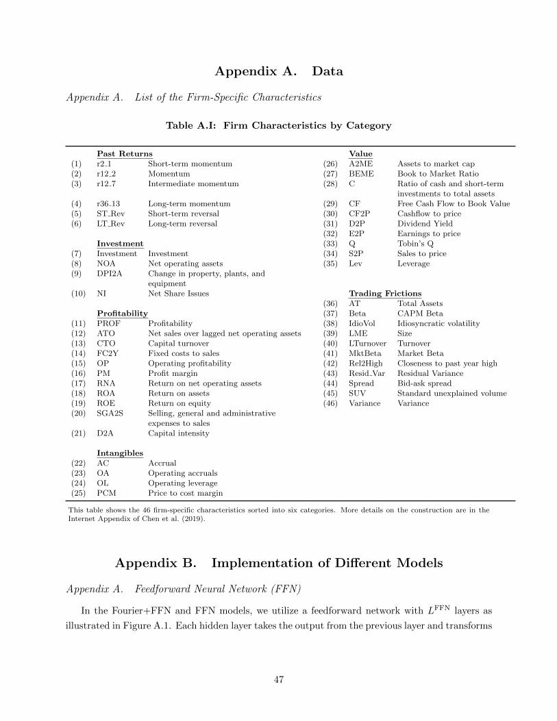
Appendix A. Data

Appendix A. List of the Firm-Specific Characteristics

Table A.I: Firm Characteristics by Category

Past Returns Value(1) r2 1 Short-term momentum (26) A2ME Assets to market cap(2) r12 2 Momentum (27) BEME Book to Market Ratio(3) r12 7 Intermediate momentum (28) C Ratio of cash and short-term

investments to total assets(4) r36 13 Long-term momentum (29) CF Free Cash Flow to Book Value(5) ST Rev Short-term reversal (30) CF2P Cashflow to price(6) LT Rev Long-term reversal (31) D2P Dividend Yield

(32) E2P Earnings to priceInvestment (33) Q Tobin’s Q

(7) Investment Investment (34) S2P Sales to price(8) NOA Net operating assets (35) Lev Leverage(9) DPI2A Change in property, plants, and

equipment(10) NI Net Share Issues Trading Frictions

(36) AT Total AssetsProfitability (37) Beta CAPM Beta

(11) PROF Profitability (38) IdioVol Idiosyncratic volatility(12) ATO Net sales over lagged net operating assets (39) LME Size(13) CTO Capital turnover (40) LTurnover Turnover(14) FC2Y Fixed costs to sales (41) MktBeta Market Beta(15) OP Operating profitability (42) Rel2High Closeness to past year high(16) PM Profit margin (43) Resid Var Residual Variance(17) RNA Return on net operating assets (44) Spread Bid-ask spread(18) ROA Return on assets (45) SUV Standard unexplained volume(19) ROE Return on equity (46) Variance Variance(20) SGA2S Selling, general and administrative

expenses to sales(21) D2A Capital intensity

Intangibles(22) AC Accrual(23) OA Operating accruals(24) OL Operating leverage(25) PCM Price to cost margin

This table shows the 46 firm-specific characteristics sorted into six categories. More details on the construction are in theInternet Appendix of Chen et al. (2019).

Appendix B. Implementation of Different Models

Appendix A. Feedforward Neural Network (FFN)

In the Fourier+FFN and FFN models, we utilize a feedforward network with LFFN layers as

illustrated in Figure A.1. Each hidden layer takes the output from the previous layer and transforms

47

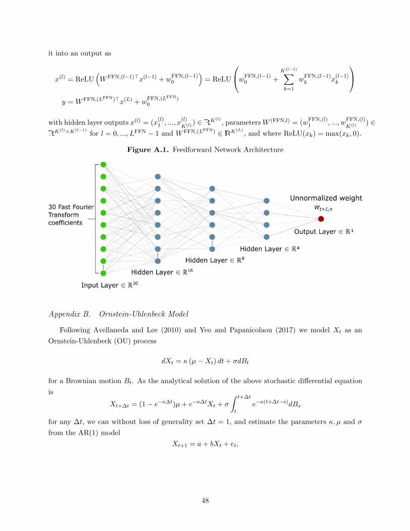
it into an output as

x(l) = ReLU(WFFN,(l−1)>x(l−1) + w

FFN,(l−1)0

)= ReLU

wFFN,(l−1)0 +

K(l−1)∑k=1

wFFN,(l−1)k x

(l−1)k

y = WFFN,(LFFN)>x(L) + w

FFN,(LFFN)0

with hidden layer outputs x(l) = (x(l)1 , ..., x

(l)

K(l)) ∈ RK(l), parametersW (FFN,l) = (w

FFN,(l)1 , ..., w

FFN,(l)

K(l) ) ∈RK(l)×K(l−1)

for l = 0, ..., LFFN − 1 and WFFN,(LFFN) ∈ RK(L), and where ReLU(xk) = max(xk, 0).

Figure A.1. Feedforward Network Architecture

Appendix B. Ornstein-Uhlenbeck Model

Following Avellaneda and Lee (2010) and Yeo and Papanicolaou (2017) we model Xt as an

Ornstein-Uhlenbeck (OU) process

dXt = κ (µ−Xt) dt+ σdBt

for a Brownian motion Bt. As the analytical solution of the above stochastic differential equation

is

Xt+∆t = (1− e−κ∆t)µ+ e−κ∆tXt + σ

∫ t+∆t

te−κ(t+∆t−s)dBs

for any ∆t, we can without loss of generality set ∆t = 1, and estimate the parameters κ, µ and σ

from the AR(1) model

Xt+1 = a+ bXt + et,

48

where each et is a normal, independent and identically distributed random variable with mean 0.

The parameters are estimated with a standard linear regression, which yields

κ = − log(b)

∆t, µ =

a

1− b,

σ√2κ

=

√σ2e

1− b2.

The strategy depends on the ratio XL−µσ√

2κ. Note that this is only defined for b < 1 which is equivalent

to parameter restrictions that the OU process is mean-reverting. The trading policy depends on the

thresholds cthresh and ccrit, which are hyperparameters. These hyperparameters are selected on the

validation data from the candidate values cthresh ∈ {1, 1.25, 1.5} and ccrit ∈ {0.25, 0.5, 0.75}. Our

benchmark model has the values cthresh = 1.25 and ccrit = 0.25, which coincides with the optimal

values in Avellaneda and Lee (2010) and Yeo and Papanicolaou (2017).

Appendix C. Convolutional Neural Network with Transformer

Appendix C.1. Convolutional Neural Network

In our empirical application, we consider a 2-layered convolutional network with some standard

technical additions. The network takes as input a window x(0) = x ∈ RL of L consecutive daily

cumulative returns or log prices of a residual, and outputs the feature matrix x ∈ RL×F given by

computing the following quantities for l = 1, . . . , L, d = 1 . . . , D

y(0)l,d = b

(0)d +

Dsize∑m=1

W(0)d,mx

(0)l−m+1, x

(1)l,d = ReLU

y(0)1,d − µ

(0)d

σ(0)d

. (A.1)

y(1)l,d = b

(1)d +

Dsize∑m=1

D∑j=1

W(1)d,j,mx

(1)l−m+1,j , x

(2)l,d = ReLU

y(1)l,d − µ

(1)d

σ(1)d

, (A.2)

xl,d = x(2)l,d + x

(0)l , (A.3)

where

µ(i)k =

1

L

L∑l=1

y(i)l,k , σ

(i)k =

√√√√ 1

L

L∑l=1

(y

(i)l,k − µ

(i)k

)2.

and b(0), b(1) ∈ RD, W (0) ∈ RD×Dsize and W (1) ∈ RD×D×Dsize are parameters to be estimated.

Compared with the simple convolutional network introduced in the main text, the previous equa-

tions incorporate three standard technical improvements commonly used in deep learning practice.

First, they include “bias terms” b(i) in the first part of equations A.1 and A.2 to allow for more

flexible modeling. Second, they include so-called “instance normalization” before each activation

function to speed up the optimization and avoid vanishing gradients caused by the saturation of

the ReLU activations. Third, they include a “residual connection” in equation A.3 to facilitate

gradient propagation during training.

49

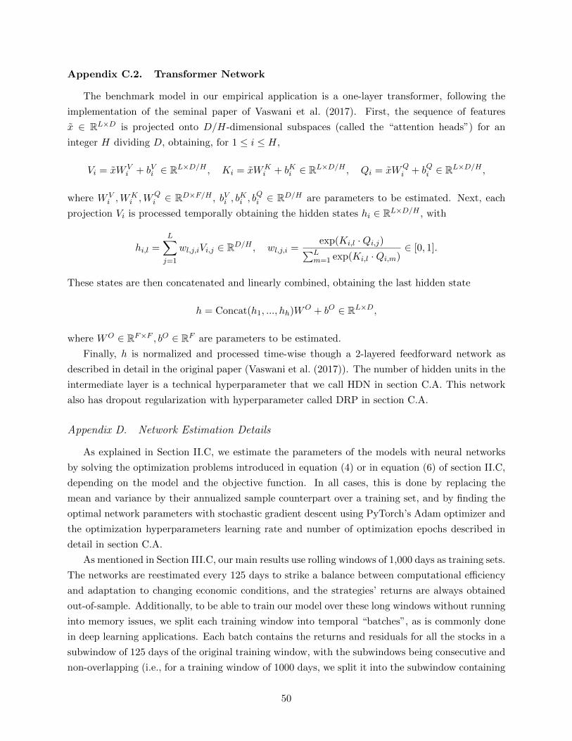
Appendix C.2. Transformer Network

The benchmark model in our empirical application is a one-layer transformer, following the

implementation of the seminal paper of Vaswani et al. (2017). First, the sequence of features

x ∈ RL×D is projected onto D/H-dimensional subspaces (called the “attention heads”) for an

integer H dividing D, obtaining, for 1 ≤ i ≤ H,

Vi = xW Vi + bVi ∈ RL×D/H , Ki = xWK

i + bKi ∈ RL×D/H , Qi = xWQi + bQi ∈ RL×D/H ,

where W Vi ,W

Ki ,W

Qi ∈ RD×F/H , bVi , b

Ki , b

Qi ∈ RD/H are parameters to be estimated. Next, each

projection Vi is processed temporally obtaining the hidden states hi ∈ RL×D/H , with

hi,l =

L∑j=1

wl,j,iVi,j ∈ RD/H , wl,j,i =exp(Ki,l ·Qi,j)∑L

m=1 exp(Ki,l ·Qi,m)∈ [0, 1].

These states are then concatenated and linearly combined, obtaining the last hidden state

h = Concat(h1, ..., hh)WO + bO ∈ RL×D,

where WO ∈ RF×F , bO ∈ RF are parameters to be estimated.

Finally, h is normalized and processed time-wise though a 2-layered feedforward network as

described in detail in the original paper (Vaswani et al. (2017)). The number of hidden units in the

intermediate layer is a technical hyperparameter that we call HDN in section C.A. This network

also has dropout regularization with hyperparameter called DRP in section C.A.

Appendix D. Network Estimation Details

As explained in Section II.C, we estimate the parameters of the models with neural networks

by solving the optimization problems introduced in equation (4) or in equation (6) of section II.C,

depending on the model and the objective function. In all cases, this is done by replacing the

mean and variance by their annualized sample counterpart over a training set, and by finding the

optimal network parameters with stochastic gradient descent using PyTorch’s Adam optimizer and

the optimization hyperparameters learning rate and number of optimization epochs described in

detail in section C.A.

As mentioned in Section III.C, our main results use rolling windows of 1,000 days as training sets.

The networks are reestimated every 125 days to strike a balance between computational efficiency

and adaptation to changing economic conditions, and the strategies’ returns are always obtained

out-of-sample. Additionally, to be able to train our model over these long windows without running

into memory issues, we split each training window into temporal “batches”, as is commonly done

in deep learning applications. Each batch contains the returns and residuals for all the stocks in a

subwindow of 125 days of the original training window, with the subwindows being consecutive and

non-overlapping (i.e., for a training window of 1000 days, we split it into the subwindow containing

50

the first 125 days, the subwindow containing the days between the 126th day and the 250th day,

etc.). The optimization process is applied successively to each batch, completing the full sequence

of batches before starting a new optimization iteration or epoch.

In the implementation of our optimization procedure under market frictions, we found it useful

to include the last allocation as an additional input to the allocation function wε, as the inclusion

of the cost term makes the objective function depend on it. However, the inclusion of the previous

allocations in either the objective function or the architecture of the model complicates the paral-

lelization of the training and evaluation computations, because after this change the model requires

the output of previous lookback window in order to compute the output of the current window. To

allow training to remain parallelized, which is desirable for reasonable computational speed given

the volume of data of our empirical application, in our implementation of the training function in

each epoch, we take the previous allocations from the output of the previous epoch and use them

as a pre-computed approximation of the allocations for the current epoch. This approximation

converges in our empirical experiments and allows us to maintain parallelization, but may produce

suboptimal results. For evaluation purposes, however, everything is computed exactly and with no

approximations using a sequential approach.

Throughout section III, all presented results have been computed with PyTorch 1.5 and have

been parallelized across 8 NVIDIA GeForce GTX Titan V GPUs, on a server with two Intel Xeon

E5-2698v3 32-core CPUs and 1 TB of RAM. The full rationale for the hyperparameter choices are

described in detail in section C.A, but for a CNN+Transformer model with a lookback window of

30 days, 8 convolutional filters with a filter size of 2, 4 attention heads, 125-day reestimation using

a rolling lookback window of 1000, it takes our deep model approximately 7 hours to be periodically

estimated and run in our 19 years of daily out-of-sample data with our universe of on average ∼550

stocks per month.

Appendix C. Additional Empirical Results

Appendix A. Robustness to Hyperparameter Selection

In this subsection, we describe our hyperparameter selection procedure and explore additional

hyperparameter choices to show that the performance of our strategies is extremely robust to our

choices. These results complement the time stability checks we exhibited in Section III.I. To decide

which hyperparameters we would select for use in our network, we fixed a validation dataset as

follows: we took the first 1000 trading days of our data set of residuals (all trading days from January

1, 1998 through December 31, 2001) of the 5-factor IPCA-based model, which is estimated with a

20-year rolling window. Because it is solely used for training in our rolling train/test procedures

used to compute strategy returns, this data is completely in-sample, and thus completely avoids

look-ahead bias which would influence any of our out-of-sample trading results in the main text. We

started with a reasonable set for our hyperparameters, and tested also additional points adjacent

51

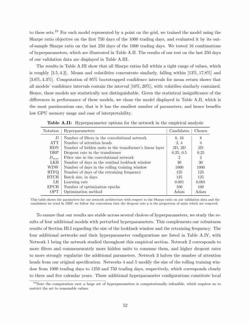
to these sets.19 For each model represented by a point on the grid, we trained the model using the

Sharpe ratio objective on the first 750 days of the 1000 trading days, and evaluated it by its out-

of-sample Sharpe ratio on the last 250 days of the 1000 trading days. We tested 16 combinations

of hyperparameters, which are illustrated in Table A.II. The results of our test on the last 250 days

of our validation data are displayed in Table A.III.

The results in Table A.III show that all Sharpe ratios fall within a tight range of values, which

is roughly [3.5, 4.2]. Means and volatilities concentrate similarly, falling within [13%, 17.8%] and

[3.6%, 4.3%]. Computation of 95% bootstrapped confidence intervals for mean return shows that

all models’ confidence intervals contain the interval [10%, 20%], with volatilies similarly contained.

Hence, these models are statistically not distinguishable. Given the statistical insignificance of the

differences in performance of these models, we chose the model displayed in Table A.II, which is

the most parsimonious one, that is it has the smallest number of parameters, and hence benefits

low GPU memory usage and ease of interpretability.

Table A.II: Hyperparameter options for the network in the empirical analysis

Notation Hyperparameters Candidates Chosen

D Number of filters in the convolutional network 8, 16 8ATT Number of attention heads 2, 4 4HDN Number of hidden units in the transformer’s linear layer 2D, 3D 2DDRP Dropout rate in the transformer 0.25, 0.5 0.25Dsize Filter size in the convolutional network 2 2LKB Number of days in the residual lookback window 30 30

WDW Number of days in the rolling training window 1000 1000RTFQ Number of days of the retraining frequency 125 125BTCH Batch size, in days 125 125

LR Learning rate 0.001 0.001EPCH Number of optimization epochs 100 100

OPT Optimization method Adam Adam

This table shows the parameters for our network architecture with respect to the Sharpe ratio on our validation data and thecandidates we tried In DRP, we follow the convention that the dropout rate p is the proportion of units which are removed.

To ensure that our results are stable across several choices of hyperparameters, we study the re-

sults of four additional models with perturbed hyperparameters. This complements our robustness

results of Section III.I regarding the size of the lookback window and the retraining frequency. The

four additional networks and their hyperparameter configurations are listed in Table A.IV, with

Network 1 being the network studied throughout this empirical section. Network 2 corresponds to

more filters and commensurately more hidden units to consume them, and higher dropout rates

to more strongly regularize the additional parameters. Network 3 halves the number of attention

heads from our original specification. Networks 4 and 5 modify the size of the rolling training win-

dow from 1000 trading days to 1250 and 750 trading days, respectively, which corresponds closely

to three and five calendar years. These additional hyperparameter configurations constitute local

19Note the computation over a large set of hyperparameters is computationally infeasible, which requires us torestrict the set to reasonable values.

52

Table A.III: Performance of candidate models on the last year of the validation data set

D ATT HDN DRP SR µ σ

8 2 2 0.25 3.81 16.3% 4.3%8 2 2 0.50 3.92 16.0% 4.1%8 2 3 0.25 3.79 16.2% 4.3%8 2 3 0.50 4.00 16.4% 4.1%8 4 2 0.25 3.81 15.6% 4.1%8 4 2 0.50 4.13 17.8% 4.3%8 4 3 0.25 3.82 15.6% 4.1%8 4 3 0.50 4.16 17.4% 4.2%16 2 2 0.25 4.00 14.8% 3.7%16 2 2 0.50 4.06 16.2% 4.0%16 2 3 0.25 4.11 14.9% 3.6%16 2 3 0.50 4.06 16.6% 4.1%16 4 2 0.25 3.93 15.6% 4.0%16 4 2 0.50 3.66 13.9% 3.8%16 4 3 0.25 4.18 16.8% 4.0%16 4 3 0.50 3.51 13.0% 3.7%

This table shows the model performance with respect to the Sharpe ratio, mean, and volatility on our validation data setfor the candidate models implied by Table A.II. The models are trained on the first three years of the validation data set(1998–2000) and tested on the last year (2001). In DRP, we follow the convention that the dropout rate p is the proportionof units which are removed.

perturbations in hyperparameter space, to which our strategies’ performance should be relatively

robust.

Table A.IV: Alternative best performing models on the data from 2002–2016

Model FLNB FLSZ ATT HDN DRP LKB WDW

Network 1 [1,8] 2 4 16 0.25 30 1000Network 2 [1,16] 2 4 32 0.5 30 1000Network 3 [1,8] 2 2 16 0.25 30 1000Network 4 [1,8] 2 4 16 0.25 30 1250Network 5 [1,8] 2 4 16 0.25 30 750

This table reports four of the best performing models for our network architecture with respect to the Sharpe ratio on our datafrom 2002–2016 and the candidates described in Table A.II. Our original network, which is studied throughout this section,is labeled as Network 1.

In Table A.V, we report the results of these models on a representative subset of 5-factor mod-

els, which are now evaluated on the full out-of-sample data. We see that the Sharpe ratios are

broadly similar across all three different perturbations of network architecture hyperparameters

(i.e., number of filters, number of attention heads, and dropout rate). The small range of values

induced by these choices shows that our network performs similarly over a variety of sensible net-

work parameters, and highlights the efficacy of our reasonable choice of convolutional, attentional,

and feedforward subnetworks which specialize in finding small temporal patterns, arranging these

patterns throughout time, and deciding on allocations based on these arranged patterns. The only

53

Table A.V: Performance of the alternative models on our benchmark residual datasets,2002–2016

Fama-French 5 PCA 5 IPCA 5

Model SR µ σ SR µ σ SR µ σ

Network 1 3.21 4.6% 1.4% 3.36 14.3% 4.2% 4.16 8.7% 2.1%Network 2 3.16 4.6% 1.4% 3.26 13.9% 4.3% 4.35 8.4% 1.9%Network 3 3.30 4.8% 1.4% 3.17 13.4% 4.2% 4.00 8.4% 2.1%Network 4 2.93 4.1% 1.4% 2.74 11.7% 4.3% 3.96 7.9% 2.0%Network 5 3.13 4.9% 1.6% 3.52 15.0% 4.3% 3.77 8.6% 2.3%

This table shows the average annualized returns, volatilities and Sharpe ratios of our alternative models from Table A.IV onour three benchmark residual datasets, trained with the Sharpe ratio objective function.

hyperparameter choice which can be considered to be slightly lower than the rest is the choice of

using a rolling training window of 1250 trading days. This suggests that statistical arbitrage poli-

cies are time-varying to adopt to changing economic conditions. Our results show that using the

latest 3 or 4 years of data for the estimation of the parameters of this model achieves an adequate

balance between capturing changing conditions and using sufficient data.

For the allocation function feedforward network (FFN) utilized for the Fourier+FFN model,

we choose a reasonable architecture based on deep learning conventions and have verified that the

results are robust to this choice. Because the input of the network are the L = 30 coefficients of the

Fourier decomposition of each residual window (X(n,t)l )1≤l≤L and the output is the corresponding

allocation weight wn,t ∈ R, we follow standard deep learning practices and consider 3 hidden

layers with dimensions 16,8,4 regularized with a dropout rate of 0.25. We use the ReLU activation

function, and train using the same procedure outlined in B.D, with the same batch size, learning

rate, number of optimization epochs, and optimization method as in Table A.II.

54

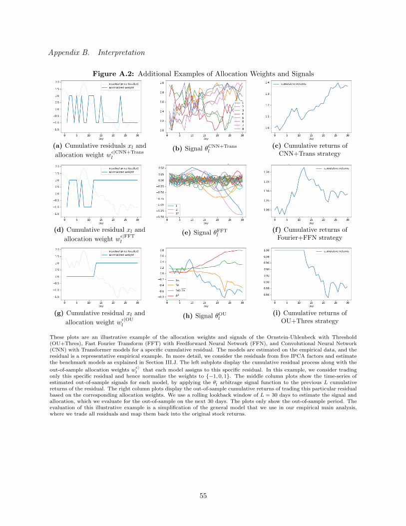
Appendix B. Interpretation

Figure A.2: Additional Examples of Allocation Weights and Signals

(a) Cumulative residuals xl and

allocation weight wε|CNN+Transl

(b) Signal θCNN+Transl

(c) Cumulative returns ofCNN+Trans strategy

(d) Cumulative residual xl and

allocation weight wε|FFTl

(e) Signal θFFTl(f) Cumulative returns of

Fourier+FFN strategy

(g) Cumulative residual xl and

allocation weight wε|OUl

(h) Signal θOUl

(i) Cumulative returns ofOU+Thres strategy

These plots are an illustrative example of the allocation weights and signals of the Ornstein-Uhlenbeck with Threshold(OU+Thres), Fast Fourier Transform (FFT) with Feedforward Neural Network (FFN), and Convolutional Neural Network(CNN) with Transformer models for a specific cumulative residual. The models are estimated on the empirical data, and theresidual is a representative empirical example. In more detail, we consider the residuals from five IPCA factors and estimatethe benchmark models as explained in Section III.J. The left subplots display the cumulative residual process along with the

out-of-sample allocation weights wε|·l that each model assigns to this specific residual. In this example, we consider trading

only this specific residual and hence normalize the weights to {−1, 0, 1}. The middle column plots show the time-series ofestimated out-of-sample signals for each model, by applying the θ·l arbitrage signal function to the previous L cumulativereturns of the residual. The right column plots display the out-of-sample cumulative returns of trading this particular residualbased on the corresponding allocation weights. We use a rolling lookback window of L = 30 days to estimate the signal andallocation, which we evaluate for the out-of-sample on the next 30 days. The plots only show the out-of-sample period. Theevaluation of this illustrative example is a simplification of the general model that we use in our empirical main analysis,where we trade all residuals and map them back into the original stock returns.

55

Figure A.3: Example Attention Weights for Sinusoidal Residual Inputs

(a) Input residual and attention head weights for ωsin = 2/30

(b) Input residual and attention head weights for ωsin = 28/30

(c) Input residual and attention head weights for ωsin = 8/30

(d) Input residual and attention head weights for ωsin = 14/30

These plots show the attention head weights of the CNN+Transformer benchmark model for simulated sinusoidal residualinput time series. The inputs are xl = sin(2πωsinl), for various ωsin and l ∈ {0, ..., 29}. The right subplot shows the attentionweights for the H = 4 attention heads for the specific residuals. The empirical benchmark model is the CNN+Transformermodel based on IPCA 5-factor residuals. We estimate the model on only once on the first Ttrain=8 years based on the Sharperatio objective.

56

Appendix C. Dependency between Arbitrage Strategies

Table A.VI: Correlations between the Returns of the CNN+Transformer Arbitrage Strategies

Fama-French 3 PCA 3 IPCA 3 Fama-French 5 PCA 5 IPCA 5 PCA 10 IPCA 10

Fama-French 3 1.00 0.32 0.44 0.62 0.25 0.43 0.21 0.44

PCA 3 0.32 1.00 0.32 0.34 0.62 0.35 0.41 0.36

IPCA 3 0.44 0.32 1.00 0.37 0.28 0.81 0.21 0.75

Fama-French 5 0.62 0.34 0.37 1.00 0.28 0.39 0.23 0.40

PCA 5 0.25 0.62 0.28 0.28 1.00 0.29 0.47 0.31

IPCA 5 0.43 0.35 0.81 0.39 0.29 1.00 0.23 0.84

PCA 10 0.21 0.41 0.21 0.23 0.47 0.23 1.00 0.25

IPCA 10 0.44 0.36 0.75 0.40 0.31 0.84 0.25 1.00

This table reports the correlations of our CNN+Transformer strategies for some representative choices of the factor models.The correlations are calculated with returns of the out-of-sample arbitrage trading from January 2002 to December 2016. Themodels are calibrated on a rolling window of four years and use the Sharpe ratio objective function. The signals are extractedfrom a rolling window of L = 30 days.

Appendix D. Time-Series Signal

In this appendix, we report the OOS returns of strategies using alternative models for the

ablation tests in Section III. For the FFN feedforward network, we use the same architecture,

hyperparameters, optimization settings, etc. as in the Fourier+FFN model utilized throughout the

empirical results section and described in Appendix C.A. For the OU+FFN model, because the

input is the low-dimensional OU signal in R4, we consider a 3 hidden layer with dimensions 4,4,4

regularized with a dropout rate of 0.25. We use the sigmoid activation function, and estimate it

using the same procedure outlined in section B.D, with the same batch size, learning rate, number

of optimization epochs, and optimization method as in Table A.II.

57

Table A.VII: OOS Annualized Performance Based on Sharpe Ratio Objective

Factors Fama-French PCA IPCA

Model K SR µ σ SR µ σ SR µ σ

0 0.50 10.6% 21.3% 0.50 10.6% 21.3% 0.50 10.6% 21.3%1 0.34 0.8% 2.3% 0.05 0.7% 11.9% 0.60 4.8% 8.0%

OU 3 0.16 0.2% 1.4% 0.44 3.4% 7.8% 0.70 4.6% 6.6%+ 5 0.17 0.2% 1.2% 0.68 4.7% 7.0% 0.66 4.2% 6.3%

FFN 8 -0.34 -0.3% 1.0% 0.51 3.1% 6.0% 0.60 3.9% 6.2%10 - - - 0.26 1.3% 5.0% 0.56 3.5% 6.2%15 - - - 0.31 1.4% 4.3% 0.54 3.3% 6.1%

0 0.57 8.8% 15.3% 0.57 8.8% 15.3% 0.57 8.8% 15.3%1 0.60 2.0% 3.3% 0.53 6.2% 11.7% 1.07 6.5% 6.1%3 1.02 2.6% 2.6% 1.15 8.2% 7.2% 1.50 7.6% 5.0%

FFN 5 1.32 2.3% 1.7% 1.42 9.8% 6.9% 1.55 7.3% 4.7%8 1.31 2.1% 1.6% 1.05 6.4% 6.2% 1.52 7.2% 4.7%10 - - - 0.70 3.5% 5.0% 1.48 7.0% 4.7%15 - - - 0.51 2.4% 4.8% 1.68 7.5% 4.5%

This table shows the out-of-sample annualized Sharpe ratio (SR), mean return (µ), and volatility (σ) of our three statisticalarbitrage models for different numbers of risk factors K, that we use to obtain the residuals. We use the daily out-of-sample residuals from January 1998 to December 2016 and evaluate the out-of-sample arbitrage trading from January 2002 toDecember 2016. OU+FFN denotes a parametric Ornstein-Uhlenbeck model to extract the signal, but a flexible feedforwardneural network to estimate the allocation function. RawFFN takes the residuals directly as signals and estimates an allocationfunction with a feedforward neural network. The deep learning models are calibrated on a rolling window of four years anduse the Sharpe ratio objective function. The signals are extracted from a rolling window of L = 30 days. The K = 0 factormodel corresponds to directly using stock returns instead of residuals for the signal and trading policy.

Appendix E. Trading Friction Results for PCA Residuals

Table A.VIII: OOS Performance of CNN+Trans with Trading Frictions

PCA factor model

Sharpe ratio Mean-variance

K SR µ σ SR µ σ

0 0.52 8.5% 16.3% 0.22 2.6% 11.9%1 0.88 7.3% 8.4% 0.79 9.0% 11.4%3 0.90 5.7% 6.3% 0.62 4.7% 7.6%5 0.81 4.5% 5.6% 0.68 4.4% 6.4%10 -0.08 -0.4% 4.8% -0.08 -0.4% 4.6%15 -0.87 -3.7% 4.3% -0.96 -3.5% 3.7%

This table shows the out-of-sample annualized Sharpe ratio (SR), mean return (µ), and volatility (σ) for the CNN+Transformermodel with trading frictions on PCA residuals. We use the daily out-of-sample residuals from January 1998 to December2016 and evaluate the out-of-sample arbitrage trading from January 2002 to December 2016. The models are calibratedon a rolling window of four years and use either the Sharpe ratio or mean-variance objective function with trading costscost(wRt−1, w

Rt−2) = 0.0005‖wRt−1 − wRt−2‖L1 + 0.0001‖min(wRt−1, 0)‖L1 . The signals are extracted from a rolling window of

L = 30 days.

58