Deep-Seated Landslides Drive Variability in Valley Width and Increase

Connectivity of Salmon Habitat in the Oregon Coast Range

Helen W. Beeson, Rebecca L. Flitcroft, Mark A. Fonstad, and Joshua J. Roering

Research Impact Statement: Deep-seated landslides promote connectivity among seasonal habitat types —spawning, summer-rearing, and winter-refuge habitat — for Coho Salmon in the Oregon Coast Range.

ABSTRACT: Declines in populations of Pacific salmon have prompted extensive and costly restoration efforts,yet many populations are still in peril. An improved understanding of landscape-scale controls on salmon habi-tat should help focus restoration resources on areas with the greatest potential to host productive habitat. Weinvestigate the contribution of deep-seated landslides (DSLs) to Coho Salmon habitat by comparing the quantityand connectivity of potential seasonal habitat observed in five streams with extensive DSLs to five lacking sig-nificant landsliding. Further, we measure valley width in these streams and relate it to connectivity. We showthat median fractions of stream length identified as spawning, summer-rearing, winter-refuge habitat, and ashaving high connectivity among seasonal habitat types are greater in streams with DSLs and that distancesbetween units of each seasonal habitat type are significantly lower in DSL terrain. The median R2 value for therelationship between drainage area and valley width is lower in landslide terrain and we observed that highconnectivity among seasonal habitat types tends to occur where valley width is variable. Our results suggestthat DSLs promote connectivity among seasonal habitat types for Coho Salmon and that prioritizing restorationprojects in streams in DSL terrain could improve the effectiveness of salmonid recovery programs.

(KEYWORDS: fish; geomorphology; fluvial processes; landslides; valley width; habitat connectivity; habitatproximity.)

INTRODUCTION

A well-accepted concept in biogeography is thatlandforms control the types and distribution of habi-tat (Swanson et al. 1988). Pacific salmon Oncor-hynchus spp. are adapted to dynamic landscapesshaped by natural disturbance processes (Mont-gomery 2000). Habitat degradation and loss as wellas overfishing and hatchery fish management haveled to precipitous declines in wild-spawning salmo-nids in the Pacific Northwest (Nehlsen et al. 1991;Montgomery 2003). Declining populations prompted

federal listing of multiple species in the 1990s, lead-ing to extensive restoration efforts (OCSRI 1997) thatrely on the identification of high-quality fish habitatand the processes that create it. Despite ongoingrestoration efforts, populations remain unstable.Although salmon are intrinsically tied to place,watershed-scale landforms are rarely included along-side the many other factors that go into planning andimplementing restoration projects. Here, we explorewhether kilometer-scale hillslope processes caninform salmonid restoration priorities.

Applying the observation that the three primarycontrols on salmon habitat are streamflow, valley

Paper No. JAWRA-17-0089-P of the Journal of the American Water Resources Association (JAWRA). Received June 29, 2017; acceptedSeptember 10, 2018. © 2018 American Water Resources Association. Discussions are open until six months from issue publication.

Department of Geological Sciences and Engineering (Beeson), University of Nevada at Reno, Reno, Nevada, USA; Pacific NorthwestResearch Station (Flitcroft), USDA Forest Service, Corvallis, Oregon, USA; and Department of Geography (Fonstad) and Department ofEarth Sciences (Roering), University of Oregon, Eugene, Oregon, USA (Correspondence to Beeson: hbeeson@nevada.unr.edus).

Citation: Beeson, H.W., R.L. Flitcroft, M.A. Fonstad, and J.J. Roering. 2018. “Deep-Seated Landslides Drive Variability in Valley Widthand Increase Connectivity of Salmon Habitat in the Oregon Coast Range.” Journal of the American Water Resources Association 54 (6):1325–1340. https://doi.org/10.1111/1752-1688.12693.

JOURNAL OF THE AMERICAN WATER RESOURCES ASSOCIATION JAWRA1325

JOURNAL OF THE AMERICAN WATER RESOURCES ASSOCIATION

Vol. 54, No. 6 AMERICAN WATER RESOURCES ASSOCIATION December 2018

constraint, and channel gradient, Burnett et al.(2007) developed species-specific intrinsic potential(IP) models of high-quality habitat for salmonids inOregon Coast Range streams, United States. A multi-year study of Coho Salmon (Oncorhynchus kisutch)populations in multiple basins in the Oregon CoastRange over time showed that Coho Salmon IP scorespredicted patterns of juvenile Coho Salmon occupancyover time (Flitcroft et al. 2014). This raises the ques-tion of what controls the distribution of areas withhigh IP, or more directly, what processes controlvalley constraint and channel gradient. Reach-scalevariations in valley width relating to tributary conflu-ences (Benda et al. 2004), and landslide deposits(May et al. 2013) are well documented, but regionaland local controls on valley width remain poorlyunderstood.

In soil-mantled landscapes, debris flows arethought to be the dominant hillslope-fluvial couplingprocess in channels with slopes >10%; these steep set-tings comprise approximately 80% of the networkrelief structure of the Oregon Coast Range (Stock andDietrich 2003). Debris flows, initiated by shallowlandsliding in colluvial hollows, are rapid, episodicevents that scour and erode low-order valleys andcan deposit large amounts of debris at tributary junc-tions (Benda 1990; Benda and Dunne 1997). Recur-rence intervals for debris flows in second-order basinshave been estimated to be a few hundred years,resulting in frequent deposition in higher orderbasins where numerous sources exist upstream(Benda and Dunne 1997; May and Gresswell 2004).The resulting deposits, known as debris flow fans, arepersistent and prevalent features in the OregonCoast Range and an important source of habitat-forming sediment and wood in streams (May andGresswell 2004; Lancaster and Casebeer 2007; Millerand Burnett 2008; Kirkby 2013).

Evidence of deep-seated landslides (DSLs) is preva-lent in 5%–25% of the Oregon Coast Range andoccurs where Eocene Tyee turbidites with abundantsiltstone layers have been exhumed and where thehillslope aspect coincides with the bedrock dip slope(Roering et al. 2005). DSLs are larger features withlonger lasting, more stable geomorphic legacies thathave the potential to create a much more substantialand persistent signature on valley and stream mor-phology than a single debris flow. DSLs have beenobserved to produce less-concave longitudinal profiles(Booth et al. 2013), knickpoints in longitudinal pro-files (Korup 2006), wider valleys (Korup et al. 2006;May et al. 2013), and in the most extreme cases, fullchannel occlusion and landslide-dammed lakes (Bald-win 1958; Korup 2005). Still, little is known aboutthe long-term effects of DSLs on fluvial processes(Korup et al. 2010). Possible initiation mechanisms

for DSLs include seismic activity, stream erosionthrough weak bedrock, and high groundwater levelsand/or precipitation caused by a wetter climate (Bald-win 1958; Hammond et al. 2009). Although there issome evidence of DSL activity within the last150 years (Burns et al. 2012), most of the DSLs inthe Oregon Coast Range are of Pleistocene age (Ham-mond et al. 2009) and Hammond et al. (2009) postu-lated that the depth of erosion suggests that somelandslides may be as old as the Pliocene. Despite theage of the DSLs, the large volume of these featuresimplies that rivers in terrain with DSLs in the Ore-gon Coast Range are still reworking sediment deliv-ered from these ancient slides.

In a recent study on Coho Salmon in the OregonCoast Range, proximity of different seasonal habitattypes (spawning, summer-rearing, and winter-refugehabitat) was found to be a better predictor of juvenilefish density than instream variables alone, highlight-ing the need to understand the processes that drivepatterns of instream connectivity or proximity amonghabitats (Flitcroft et al. 2012). May et al. (2013)showed that anomalously wide valleys exist upstreamfrom and adjacent to two discrete DSLs (isolatedslope failures) and that these areas had high IP forCoho Salmon owing to the lack of valley constraint.We expand on the work by May et al. (2013) by inves-tigating the geomorphic effects of extensive deep-seated landsliding, which we define as slope failure ofthe majority of hillslopes in a given watershed — aphenomenon that is prevalent in the Oregon CoastRange (Roering et al. 2005). We explore how the pres-ence of extensive deep-seated landsliding affects val-ley floor width and the quantity and connectivity ofseasonal habitat for Coho Salmon by comparing thesemetrics in five subbasins in the Umpqua River Basinwith extensive DSLs to five subbasins in the UmpquaRiver Basin without deep-seated landsides. Wehypothesize that DSLs promote variable valley widthand hence a higher frequency of anomalously widevalleys and that this results in greater connectivitybetween seasonal habitat types.

STUDY AREA

The central Oregon Coast Range is an ideal placeto study the effects of DSLs on Coho Salmon habitatbecause (1) landslides are abundant in an area withotherwise relatively uniform topography and lithology(Heller and Dickinson 1985) and (2) stream habitatsurvey data taken explicitly in light of Coho Salmonlife cycle needs (Moore et al. 1997, 2007) are avail-able from the Oregon Department of Fish and

JAWRA JOURNAL OF THE AMERICAN WATER RESOURCES ASSOCIATION1326

BEESON, FLITCROFT, FONSTAD, AND ROERING

Wildlife (ODFW) Aquatic Inventories Project (AIP)for numerous basins across the region.

We chose to conduct our study in the UmpquaRiver Basin because it is the basin most compre-hensively surveyed for Coho Salmon habitat by theAIP in the Oregon Coast Range and limiting thestudy to one basin mitigates for interbasin variabil-ity at a broad scale. The Umpqua River Basincrosses through the Oregon Coast Range with aportion of the system draining from the CascadeMountains. Therefore, we focused on the portion ofthe Umpqua River Basin contained in the OregonCoast Range. Within this area, we selected all ofthe subbasins that met the following criteria: (1)available fish habitat survey data from a subset ofyears that have been subject to quality control test-ing (see Methods); (2) either extensive DSLs or uni-formly steep and dissected (USD) valley-ridgetopography (see Methods); and (3) available LightDetection and Ranging (lidar) data. This resulted in

five streams in DSL terrain (Halfway, Sand, Rock,Scare, and Yellow Creeks) and five streams withoutDSLs (Charlotte, Dean, Herb, Scholfield, and Swe-den Creeks) (Figure 1 and Table 1). We excluded asmall basin (Little Sand Creek) that is a subbasinof a larger one that we included (Big Sand Creek)because none of the other streams had surveyedtributaries.

The selected subbasins have comparable surfacegeology, occurring in the extensive region underlainby the Tyee Formation, an Eocene-age, relativelyundeformed sandstone and siltstone layer with mini-mal facies variation (Heller and Dickinson 1985). Cli-mate is temperate maritime throughout the OregonCoast Range, and hence can be assumed to vary min-imally among subbasins. Douglas-fir forest blanketsthe mountains, but throughout the central OregonCoast Range stand composition has been altered bylogging and land use to a landscape dominated byyounger stands (Kennedy and Spies 2004). Land use

25 km

Oregon

Umpqua basinHerb Creek

Sweden Creek

Dean Creek

Charlotte Creek

Scholfield Creek

Scare Creek

Halfway Creek

Yellow Creek

Big Sand Creek RockCreek

Fig

. 2A&

C

Fig. 2B&D

Umpqua River Basin

Deep-seated landslides

Streams in deep-seated landslide terrain

Streams in uniformly steep and dissected terrain

Umpqua River basin boundary

Tyee formation

Mainstem Umpqua River

FIGURE 1. Location of the 10 streams in the Umpqua River Basin, used for an assessment of CohoSalmon habitat connectivity and the presence (or absence) of deep-seated landslides (DSLs).

JOURNAL OF THE AMERICAN WATER RESOURCES ASSOCIATION JAWRA1327

DEEP-SEATED LANDSLIDES DRIVE VARIABILITY IN VALLEY WIDTH AND INCREASE CONNECTIVITY OF SALMON HABITAT IN THE OREGON COAST RANGE

in the study subbasins is predominantly evergreenforest, mixed forest, and shrub/scrub (Table 1, Homeret al. 2015).

METHODS

Identifying Extensive DSLs

To locate DSLs, we used the automated algorithmdeveloped by Roering et al. (2005) that exploits therelationship between curvature and slope that ischaracteristic of DSLs. We used the algorithmthreshold that was shown to be consistently accu-rate at delineating DSL masses that were also iden-tified using aerial photos, field observations, andtopographic maps (Roering et al. 2005). Subbasinscharacterized as occurring in “DSL terrain” areaffected by extensive deep-seated landsliding (slopefailure of the majority of at least one side of thevalley). These basins are less uniformly dissected bystream networks and have more irregular hillslopegradients (and broad, gentle hillslopes) than basinsin the Oregon Coast Range with no DSLs (Fig-ure 2). Subbasins chosen as controls have no slopesmapped as DSL masses and have USD valley-ridgetopography. Hereafter we refer to the deep-seated

landslide terrain as DSL terrain and the controlgroup in uniformly steep and dissected terrain asUSD terrain.

Identifying Potential Seasonal Habitat andCalculating Habitat Connectivity

Seasonal habitat data were acquired from theODFW AIP. The AIP provides quantitative data onstream habitat conditions for Oregon streams. Thesurvey methods employed by the AIP involve system-atically identifying and measuring stream geomor-phic features in the field as the surveyors walkupstream. Different habitat units are identified (i.e.,pool, riffle, glide) and characteristics of substrate areestimated while modal depth is measured. Channelwidth and unit length were measured every 10thhabitat unit providing a means to calibrate all esti-mated lengths. Geomorphic features and measure-ments are georeferenced, allowing for distancedownstream and habitat unit lengths to be calculatedin a geographic information system (GIS) (Mooreet al. 1997, 2007). A robust literature using AIP fieldsurvey data has demonstrated the relevance and util-ity of this methodology to explain patterns of CohoSalmon occupancy (Steel et al. 2012; Flitcroft et al.2014), to describe relationships between instreamhabitat and landscape conditions (Anlauf et al. 2011),

TABLE 1. Study subbasins in the Umpqua River Basin.

Stream

name

Drainage

areassurveyed

(km2)

Total

drainage

area inbasin

(km2)

Mainstem

stream

lengthsurveyed

(km)

Mainstem

total

streamlength

(km)

Elevation

range (m)

Vegetation

type

Distance tocoast from

outlet (km)

Mean

annualprecipitation

(mm)

Yearsurveyed

by AIP

Streams in USD terrain

Charlotte Creek 0.5–9.9 9.9 5.5 5.5 1–563 Evergreen forest 28.4 2,455 1993

Dean Creek 2.5–34.4 34.4 10.9 12.1 6–1,600 Evergreen forest,Mixed forest

21.2 2,272 1994

Herb Creek 1.0–6.3 6.8 4.4 4.8 319–1,333 Evergreen forest,

Mixed forest

45.0 1,814 1994

Scholfield Creek 4.9–57.8 57.8 25.3 28.4 0–537 Evergreen forest,

Mixed forest,

Shrub/scrub

12.2 2,008 1994

Sweden Creek 0.7–5.2 5.2 3.5 3.7 367–1,512 Evergreen forest,

Mixed forest

45.5 1,779 1994

Streams in DSL terrain

Halfway Creek 0.5–20.0 20.0 13.1 13.1 490–1,792 Evergreen forest 52.2 1,467 1994

Rock Creek 1.8–15.4 13.5 10.1 10.4 98–363 Shrub/scrub,

Evergreen forest

78.5 1,255 1995

Big Sand Creek 1.1–35.3 35.3 10.8 11.3 315–1,495 Shrub/scrub,

Evergreen forest

78.0 1,283 1993

Scare Creek 2.6–14.7 14.8 7.6 9.7 204–1,761 Evergreen forest,

Mixed forest,

Shrub/scrub

38.6 1,841 1994

Yellow Creek 0.5–50.2 52.5 15.2 15.2 245–2,458 Evergreen forest 67.3 1,220 1994

Note: AIP, Aquatic Inventories Project; USD, uniformly steep and dissected.

JAWRA JOURNAL OF THE AMERICAN WATER RESOURCES ASSOCIATION1328

BEESON, FLITCROFT, FONSTAD, AND ROERING

and to understand patterns of juvenile Coho Salmonhabitat use (Steel et al. 2016).

In this study, we utilize AIP instream habitat dataon habitat units, residual pool depth (maximum pooldepth minus pool tail crest, e.g., Hilton and Lisle1993), and percent cover of silt/organics. Comprehen-sive, census-style stream habitat survey data thatcaptures stream conditions during a similar windowof time across a basin are rare. We were able toacquire survey data for this study that were collectedduring mid-summer (July–August) 1993–1995. Ideally,we would have used field data collected synchronouslywith available lidar imagery used in the geomorphicassessment of valley width. While there is a gapbetween the time of the field survey and lidar dataacquisition, the geomorphic features captured by lidarare likely to be semipermanent geomorphic featureswith respect to instream habitat. Therefore, the“snapshot” of stream conditions collected by the fieldsurvey is still relevant to explore relationshipsbetween geomorphic conditions and fish habitat.Although stream survey methods are systematic and

survey training occurs annually, there is always somelevel of uncertainty among survey professionals. Per-formance of the AIP survey methodology comparessimilarly with respect to other habitat survey pro-grams for repeatability and accuracy of measurements(Roper et al. 2010). Concern regarding inconsistencyof field measurements in field habitat surveys hasbeen presented in the literature generally, andregarding sediment (Olsen et al. 2005; Faustini andKaufmann 2007) and habitat typing in particular(Poole et al. 1997). For the purposes of our research,the evidence that the AIP surveys are generallystrong at identification of habitat types (Roper et al.2010), and that pool depth was a measured attribute,made this dataset adequate to the main purpose ofour effort (Table 2). Development of stream habitatsurvey methods with high repeatability and consis-tency are being developed with remotely sensed tools(i.e., green lidar), but are not currently available.

Coho Salmon use different habitats seasonally inresponse to life-stage needs (Groot and Margolis1991; Nickelson et al. 1992). In the autumn, spawn-ing Coho Salmon lay their eggs in riffles in the inter-stitial spaces in gravel. After they hatch, CohoSalmon fry migrate to slow water to feed, grow, andseek thermal refuge during the summer. In the win-ter, off-channel habitat provides refuge from high-flow events. Based on these life cycle needs (Grootand Margolis 1991), adequate potential habitat forCoho Salmon for spawning, summer-rearing, andwinter-refuge can be identified by querying thestream survey data for specific criteria. We identifiedhabitat variables known to be biologically relevantfor different life stages (sensu Flitcroft et al. 2014;Flitcroft et al. 2016). Coho Salmon are known to needgravel for spawning (Groot and Margolis 1991; Bilbyand Bisson 1998). Fine-grained sediment is known todecrease juvenile survival to emergence (Bryce et al.2008, 2010) and off-channel habitat has been identi-fied as important refuge for juveniles to survive

Deep-seated landslides1 kmGradient

High : 9.0

Low : 0.001

Yellow Creeka b

c d

Dean Creek

FIGURE 2. Examples of USD terrain (a, c) and terrain shaped byDSLs (b, d). (a) Hillshade of Dean Creek. (b) Hillshade of YellowCreek with DSLs shown in light red. (c) Gradient of Dean Creek withUSD hillslopes. (d) Gradient of Yellow Creek with irregular andoverall low hillslope gradients. See extent indicators in Figure 1 forlocations.

TABLE 2. Criteria used for characterizing habitat units aspotential Coho Salmon seasonal habitat types from the Oregon

Department of Fish and Wildlife AIP stream survey data.

Potential habitattype Criteria

Spawning habitat Riffles with ≥50% gravel and ≤8% silt/organicsSummer-rearinghabitat

Pools with residual pool depth (depth minuspool tail crest depth):≥0.5 m deep in streams <7 m wetted width≥0.6 for streams 7–15 m wetted width≥1 m deep in streams >15 m wetted width

Winter-refugehabitat

Habitats identified peripheral to, or off themainstem that become slower water-refugehabitats during high-flow events:backwaters, alcoves, and isolated pools

JOURNAL OF THE AMERICAN WATER RESOURCES ASSOCIATION JAWRA1329

DEEP-SEATED LANDSLIDES DRIVE VARIABILITY IN VALLEY WIDTH AND INCREASE CONNECTIVITY OF SALMON HABITAT IN THE OREGON COAST RANGE

winter storm events (Nickelson et al. 1992). Evalua-tion of the AIP field survey dataset allowed us toidentify habitat characteristics that would generallyrepresent these life-stage habitat needs (Table 2).The percent cover of silt/organics is assessed visuallyand, given the low threshold needed for a unit toqualify as potential spawning habitat (Table 2), istherefore a source of uncertainty in our analysis. Toaddress this uncertainty, we include a secondaryanalysis using a threshold of 16% silt/organics toidentify potential spawning habitat.

Connectivity between seasonal habitats is as impor-tant as habitat quality for individual life stages ofCoho Salmon (Flitcroft et al. 2012). Therefore, we cal-culated the distance from each surveyed habitat unitto each of the nearest types of seasonal habitat.Because each habitat unit is a unique length, weincluded the length of the unit in question (Figure 3)such that the resulting distance represents the maxi-mum distance a fish would have to travel betweenhabitat units. Although the actual distance a fishmight travel could be shorter, especially in the case oflong habitat units, this approach reduces the potentialto overestimate connectivity. This approach does notcapture interannual variation of water depth or chem-istry that have the potential to alter connectivityamong sites (i.e., shallow water limiting passage).

We based our assessment of habitat proximity onthe maximum recorded distance of 234 m traveled byjuvenile Coho Salmon in the summer (Kahler et al.2001). Therefore, we identified potential spawninghabitat and potential summer-rearing habitat thatwere less than 250 m apart and classified habitatunits between them as part of a high-connectivityreach (Figure 3). Juvenile Coho Salmon are observedto exhibit high fidelity to winter-refuge habitat (Bellet al. 2001; Ebersole et al. 2006). However, in otherportions of their range, juvenile Coho Salmon are

known to move extensive distances for feeding coinci-dent with available food sources and thermal condi-tions (Armstrong and Schindler 2013). In the OregonCoast Range, Flitcroft et al. (2012) observed thatjuvenile fish abundances in summer were substan-tially higher at sample sites that were within 500 mfrom spawning, summer, or winter habitat. Thus, weclassified units of a high-connectivity reach that alsohad potential winter-refuge habitat within 250 m, aswell as the units connecting the high-connectivityreach with the winter habitat, as part of a “compre-hensive patch” (Figure 3). The choice of 250 m inthese calculations results in comprehensive patch dis-tances between potential summer-rearing and poten-tial winter-refuge habitat below 500 m, thus withinthe threshold observed by Flitcroft et al. (2012). Todetermine whether our results were dependent onthe distances chosen for the analysis, we performedthe same calculations with half the original distances(125 and 250 m) and twice the original distances(500 m and 1 km) (see Supporting Information). Thealgorithm used to calculate minimum distances toeach type of potential seasonal habitat and resultingconnectivity among habitat types is available as Sup-porting Information.

For each stream, we summed stream length foreach potential seasonal habitat resulting in threedatasets. Additionally, we summed stream lengthcharacterized as a high-connectivity reach (linkingpotential spawning and summer-rearing habitat), oras a comprehensive patch (connectivity among allthree seasonal habitats). We then calculated thefraction of total stream length for each of these,resulting in two more datasets. We grouped streamsas occurring in DSL terrain or USD terrain andobserved that the grouped fractions of stream lengthwere not normally distributed. We tested for equalvariances using a Brown–Forsythe test and used aMann–Whitney–Wilcoxon test on datasets with equalvariance to determine whether differences betweengroups were statistically significant (a = 0.05). TheMann–Whitney–Wilcoxon test is a nonparametricstatistical test that does not assume normal distribu-tion but does assume equal variance. The Mann–Whitney–Wilcoxon also assumes independence, anassumption that may be violated by spatial autocor-relation given the proximity between some samplestreams. Given that we selected all subbasins thatmet the criteria presented above, eliminatingstreams based on proximity to other study subbasinswould have severely limited the number of samplesin each group. We report and compare the medianand the median absolute deviation (MAD) for eachgroup of streams for each category assessed.

To explore how the distribution of potential sea-sonal habitat types differs between groups, we

Comprehensive Patch

Highly Connected

Not connected

Potential spawning habitatPotential summer refuge habitatPotential winter refuge habitat

250 m

250 m

250 m

FIGURE 3. Characterization of potential seasonal habitat connec-tivity. Habitat units connecting potential spawning habitat withpotential summer habitat were characterized as having high con-nectivity if the spawning and summer habitats were within 250 mof each other. If potential winter-refuge habitats were within250 m of any of the high-connectivity units, all the connected habi-tat units were characterized as a “comprehensive patch.”

JAWRA JOURNAL OF THE AMERICAN WATER RESOURCES ASSOCIATION1330

BEESON, FLITCROFT, FONSTAD, AND ROERING

compared the distances to the nearest type of eachpotential seasonal habitat. For all habitat units ineach stream, we calculated the distance to the near-est potential spawning, summer-rearing, and winter-refuge habitats. We combined all the minimumdistances for each group for each seasonal habitattype such that each group (USD and DSL) had threedatasets of minimum distances. Although these sixdatasets were not normally distributed, the samplesets were large enough (n = 1,083 and 2,902 for USDand DSL streams, respectively) such that a two-sam-ple unpaired t-test was appropriate to determine ifthe minimum distances differed significantly(a = 0.05) between groups for each seasonal habitattype. We used a Welch’s t-test, an alternative to theStudent’s t-test that does not assume equal variances.We report the mean with the results of the t-test aswell as the median and MAD.

Measuring Valley Floor Width

We used 1-m resolution airborne data (lidar),acquired from the Oregon Department of Geology andMineral Industries, to measure valley floor width in aGIS. We first used a 15 9 15 m moving window algo-rithm to smooth the lidar and calculate gradient froma fitted second-order polynomial (Wood 1996) (Fig-ure 2c, 2d). Smoothing resulted in less variability inslope such that the valley–hillslope transition waseasily defined by a break in slope (Figure 2c, 2d).Using a combination of the gradient layers and hill-shades derived from the lidar in a GIS, we manuallymeasured the valley widths along the mainstemevery 100 m in all subbasins at cross sections perpen-dicular to the valley walls. We used an eight-directionmodel to route flow on unsmoothed lidar in order tocalculate drainage area at each point. In all studysubbasins except Scholfield Creek, we measured val-ley widths from a drainage area of 1 km2 to the samedownstream drainage area as AIP survey data, whichin all basins starts at the stream’s confluence with alarger river (generally either the mainstem Umpquaor the North Fork Smith). In Scholfield Creek, wemeasured valley widths only above the head of tide toavoid conflating hillslope processes with coastalprocesses.

Valley widening may occur at tributary junctionsfrom the accumulation of flood or debris flow deposits(Benda et al. 2004). Because extensive DSLs caninfluence the number and location of confluences, toavoid conflating landslide effects on confluences withlandslide effects on valley width, we excluded allpoints where valleys were wider at confluences aswell as points upstream or downstream that fellwhere valleys remained anomalously wide. Thus, our

valley width measurements only reflect the directeffect of DSLs on the width of the primary valley.Large confluences resulted in more skipped pointsand small confluences resulted in a negligible numberof excluded points. To understand how the exclusionof these data may have influenced our results, wedocumented the fraction of stream length where val-ley width measurements were bypassed because ofconfluences and tested whether the fractions differedsignificantly between groups with a Mann–Whitney–Wilcoxon test (a = 0.05). Further, we characterizedhigh-connectivity reaches and comprehensive patchesas being associated with a confluence if the reach/patch began at a measurement that was excludedbecause of confluence effects and did not extendmore than 200 m upstream or downstream of theconfluence.

Using the same groupings of streams as were usedfor the analysis of potential seasonal habitat (streamsin USD terrain vs. those with DSLs), we assessedwhether the relationships between valley floor widthand drainage area differed between the two groups.First, we fit power functions to the relationshipsbetween valley floor width and drainage area foreach stream. Because measurements were madealong mainstems, the R2 value of the best-fit powerfunction reflects longitudinal variability in valleywidth and the exponent of the best-fit power functionreflects how rapidly valley width changes as drainagearea increases or decreases. The distributions of val-ley width-drainage area R2 values and valley width-drainage area exponents are both non-normal. Wetested for equal variance using the Brown–Forsythetest and, because variances were not significantlydifferent (see Results), we used a Mann–Whitney–Wilcoxon test to determine if values were signifi-cantly different between groups (a = 0.05).

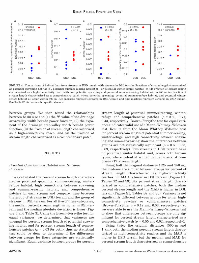
At each valley width measurement, we recordedwhether a high-connectivity reach or a comprehen-sive patch crosses the point in question and whethervalleys are wider than the best-fit power function fordrainage area-valley width predicts. To investigatethe parameters that influence connectivity, we plot-ted the relationships between the fractions of streamlength characterized as high-connectivity reaches andcomprehensive patches and the R2 values of the best-fit power functions, the exponents of the best-fitpower functions, and the median minimum distancesto potential spawning, summer-rearing, and winter-refuge habitat.

Lastly, to explore whether basin size influencedour results, we used a Brown–Forsythe test forequal variance and, because variances did not dif-fer significantly between groups (see Results), aMann–Whitney–Wilcoxon test to determine if theselected basins differed significantly (a = 0.05) in size

JOURNAL OF THE AMERICAN WATER RESOURCES ASSOCIATION JAWRA1331

DEEP-SEATED LANDSLIDES DRIVE VARIABILITY IN VALLEY WIDTH AND INCREASE CONNECTIVITY OF SALMON HABITAT IN THE OREGON COAST RANGE

between groups. We then tested the relationshipsbetween basin size and (1) the R2 value of the drainagearea-valley width best-fit power function, (2) the expo-nent of the drainage area-valley width best-fit powerfunction, (3) the fraction of stream length characterizedas a high-connectivity reach, and (4) the fraction ofstream length characterized as a comprehensive patch.

RESULTS

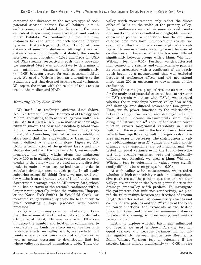
Potential Coho Salmon Habitat and HillslopeProcesses

We calculated the percent stream length character-ized as potential spawning, summer-rearing, winter-refuge habitat, high connectivity between spawningand summer-rearing habitat, and comprehensivepatches for each stream and compare these betweenthe group of streams in USD terrain and the group ofstreams in DSL terrain. For all five of these categories,the median percent stream length is higher in DSL ter-rain and the median absolute deviation is lower (Fig-ure 4 and Table 3). Using the Brown–Forsythe test forequal variances, we determined that variances areunequal for percent stream length of potential spawn-ing habitat and for percent stream length of compre-hensive patches (p = 0.03 for both), thus no statisticaltest could be done to determine if the differencesbetween groups for these categories are statisticallysignificant. Equal variance between groups for percent

stream length of potential summer-rearing, winter-refuge and comprehensive patches (p = 0.69, 0.71,0.43, respectively, Brown–Forsythe test for equal vari-ance) indicates valid use of a Mann–Whitney–Wilcoxontest. Results from the Mann–Whitney–Wilcoxon testfor percent stream length of potential summer-rearing,winter-refuge, and high connectivity between spawn-ing and summer-rearing show the differences betweengroups are not statistically significant (p = 0.69, 0.53,0.69, respectively). Two streams in USD terrain haveno potential winter habitat and, across both terraintypes, where potential winter habitat exists, it com-prises <1% stream length.

Using half the original distances (125 and 250 m),the medians are similar between groups for percent ofstream length characterized as high-connectivityreaches but MAD is lower in DSL terrain (Figure S1,Tables S2 and S3). For percent stream length charac-terized as comprehensive patches, both the medianpercent stream length and the MAD is higher in DSLterrain (Figure S1, Tables S2 and S3). Variance is notsignificantly different between groups for either high-connectivity reaches or comprehensive patches(Brown–Forsythe, p = 0.19 and 0.06, respectively), sowe were able to use the Mann–Whitney–Wilcoxon testto show that differences between groups are only sig-nificant for percent stream length characterized as acomprehensive patch (p = 0.55 and 0.02, respectively).

Using twice the original distances (500 m and1 km), both the median percent stream length charac-terized as high-connectivity reaches and the MAD ishigher in USD terrain but the median and MAD forpercent stream length characterized as comprehensive

Spa

wni

ng h

abita

t

0

0.02

0.04

0.06

0.08

0.1

0.12

0.14

0.16

0.18

Sum

mer

hab

itat

0

0.1

0.2

0.3

0.4

0.5

0.6

0.7

Win

ter

habi

tat

0

0.001

0.002

0.003

0.004

0.005

0.006

0.007

0.008

0.009

0.01

Spa

wni

ng-s

umm

er r

efug

e co

nnec

tivity

0.1

0.15

0.2

0.25

0.3

0.35

0.4

0.45

0.5

Com

preh

ensi

ve p

atch

0

0.05

0.1

0.15

0.2

0.25

0.3

0.35

0.4

0.45unequalvariance

p = 0.69U = 15

a b c

p = 0.69U = 15

d e

p = 0.53U = 16

unequalvariance

USD DSL

Fra

ctio

n o

f st

ream

len

gth

ch

arac

teri

zed

as

USD DSL USD DSL USD DSL USD DSL

FIGURE 4. Comparisons of habitat data from streams in USD terrain with streams in DSL terrain. Fractions of stream length characterizedas potential spawning habitat (a), potential summer-rearing habitat (b), or potential winter-refuge habitat (c). (d) Fraction of stream lengthcharacterized as a high-connectivity reach with both potential spawning and potential summer-rearing habitat within 250 m. (e) Fraction ofstream length characterized as a comprehensive patch where potential spawning, potential summer-refuge habitat, and potential winter-refuge habitat all occur within 500 m. Red markers represent streams in DSL terrain and blue markers represent streams in USD terrain.See Table S1 for values for specific streams.

JAWRA JOURNAL OF THE AMERICAN WATER RESOURCES ASSOCIATION1332

BEESON, FLITCROFT, FONSTAD, AND ROERING

patches is higher in DSL terrain (Figure S2,Tables S2 and S3). Variance is not significantly differ-ent between groups for percent stream length of high-connectivity reaches but it is significantly different forpercent stream length of comprehensive patches(Brown–Forsythe, p = 0.08 and 0.01, respectively).Thus, no statistical test was performed on percentstream length characterized as comprehensive patchesand the difference between groups for high-connectiv-ity reaches is not significantly different betweengroups (p = 0.10; Mann–Whitney–Wilcoxon test).

To explore how the distribution of seasonal habitattypes differed between terrain types, we compared theminimum distances to potential spawning, summer-rearing, and winter-refuge habitat between groupssuch that each category contains values from all habi-tat units in all five basins within that group (Figure 5).The differences between groups are significant for allthree categories — potential spawning, summer-rear-ing, and winter-refuge habitat (p < 0.001; Welch’s two-sample unpaired t-test) (Figure 5). Mean minimumdistance to spawning habitat is 444 m in DSL terraincompared with 615 m in USD terrain, mean minimumdistance to summer-rearing habitat is 60 m in DSLterrain compared with 77 m in USD terrain, and themean minimum distance to winter-refuge habitat is1,366 m in DSL terrain compared with 3,471 m inUSD terrain. The median minimum distances and theMAD are also lower in DSL terrain for all three typesof potential habitat (Table 3).

In all the above analyses, potential spawning habi-tat was defined as riffles with ≥50% gravel and ≤8%silt/organics. Because the percent cover of silt/organ-ics is visually assessed according to the AIP protocoland thus potentially subject to high levels of uncer-tainty, we conducted the same analyses with spawn-ing habitat defined as riffles with ≥50% gravel but≤16% silt/organics. The difference in the thresholdused for silt/organics did not change the results (Fig-ure S3, Tables S4 and S5).

Valley Floor Width, Hillslope Processes, and HabitatConnectivity

The strength of the relationship between valleyfloor width and drainage area reflects longitudinalvariability in valley width because measurementswere made along mainstems and drainage areachanges monotonically with stream length. Three outof five basins in DSL terrain exhibit weaker relation-ships (lower R2 values) between valley floor widthand drainage area when compared to basins in USDterrain without DSLs (Figure 6), but R2 values arenot significantly different between the group ofstreams in DSL terrain and the group of streams in

TABLE

3.Summary

ofresu

ltsforseasonalhabitat/connectivityanalysisandvalley

width/con

nectivityanalysis.

Percent

stream

length

spawnin

g

Percent

stream

length

summer

Percent

stream

length

win

ter

Percent

stream

length

HC

Percent

stream

length

CP

Min

imum

dista

nce

to

spawnin

g

(m)

Min

imum

dista

nce

to

summer

(m)

Min

imum

dista

nce

to

win

ter(m

)

DA-V

W

R2

DA-V

W

exp

Percent

HC

with

wid

eVW

Percent

CP

with

wid

e

VW

Percent

stream

length

exclu

ded

by

confluences

PercentHC

influenced

by

confluences

PercentCP

influenced

by

confluences

Med

ian

(MAD)

USD

2.32(1.05)

16.53(8.87)

0.12(0.12)

28.16(8.11)

0.00(0.00)

338(247)

52(29)

3,161(2,291)

0.51(0.12)

0.62(0.25)

47(10)

50(0)

18(2)

0(0)

0(0)

Med

ian

(MAD)

DSL

9.16(0.63)

25.89(4.97)

0.36(0.07)

31.80(4.14)

21.76(5.10)

118(101)

40(23)

475(351)

0.41(0.29)

0.60(0.25)

58(17)

61(9)

11(1)

13(1)

0(0)

Notes:MAD,med

ianabsolute

dev

iation

;DA,drainagearea;HC,highconnectivity;CP,comprehen

sivepatches;VW,valley

width.

Values

forea

chsu

bbasin

are

reportedin

Table

S1.PercentHC

withwideVW

refers

tothepercentof

valley

width

mea

suremen

tswithhighconnectivitybetweensp

awningand

summer-rea

ringhabitatthathadvalley

width

mea

suremen

tsthatex

ceed

edthewidth

predictedbythebest-fitpow

erfunction.PercentCP

withwideVW

istheanalogou

smea

-su

remen

tbutwithcomprehen

sivepatches.

JOURNAL OF THE AMERICAN WATER RESOURCES ASSOCIATION JAWRA1333

DEEP-SEATED LANDSLIDES DRIVE VARIABILITY IN VALLEY WIDTH AND INCREASE CONNECTIVITY OF SALMON HABITAT IN THE OREGON COAST RANGE

USD terrain (p = 0.29, Brown–Forsythe test for equalvariance; p = 0.8, Mann–Whitney–Wilcoxon test). Themedian R2 value for the relationships between valleyfloor width and drainage area is lower in DSL terraincompared with USD terrain (0.41 vs. 0.51, respec-tively) and the MAD in R2 values is higher in DSLterrain compared with USD terrain (0.29 vs. 0.12,respectively) (Table 3).

The exponent in the drainage area-valley widthpower function reflects the rate at which valley widthchanges with drainage area. The larger basins in DSLterrain have smaller exponents of the best-fit powerfunctions than basins of comparable size in USD terrain(Figure 6), but again the difference between groups isnot statistically significant (p = 0.16, Brown–Forsythetest for equal variance; p = 0.3, Mann–Whitney–Wil-coxon test). The median exponents are similar betweengroups (0.62 vs. 0.60) as are the MADs (0.25 for both).The two basins with the smallest exponents (Scare andYellow Creeks) have valley widths similar to other sam-ple creeks at low drainage area but more narrow valleysat large drainage areas (Figure 6).

The percent of stream length excluded from ourvalley width measurements because of widening atconfluences did not differ significantly between DSLand USD terrain (p = 0.12, Brown–Forsythe test forequal variances; p = 0.2, Mann–Whitney–Wilcoxontest). However, the percent of stream length excludedis higher in USD terrain, with a median of 18%

excluded in USD terrain compared with 11%excluded in DSL terrain (Table 3). The MAD in thepercent of stream length excluded is only slightlyhigher in USD terrain — 2% compared with 1% inDSL terrain. Few streams have high-connectivityreaches associated with confluences and/or compre-hensive patches associated with confluences(Table S1) such that no valid statistical test for differ-ences between groups could be performed. Althoughthe majority of high-connectivity reaches and compre-hensive patches were not deemed as associated withconfluences in either terrain type, many high-connec-tivity reaches and comprehensive patches cross smallconfluences and continue upstream and/or down-stream much more than 200 m.

Across both terrain types, 56% of reaches charac-terized as having high connectivity between potentialspawning and summer-rearing habitat and 57% ofreaches characterized as comprehensive patchesoccur in areas with valleys wider than predicted bythe best-fit power function (Figure 6 and Table S1).Both types of high-connectivity categories, but com-prehensive patches in particular, appear to occur inlocations where valley width changes rapidly eitherupstream or downstream (Figure 6). The two basinswith the highest fraction of stream length character-ized with high connectivity were Halfway Creek andYellow Creek, both in terrain dominated by extensivedeep-seated landsliding (Figure 6 and Table 3).

Min

imum

dis

tanc

e to

spa

wni

ng h

abita

t (m

)

0

1000

2000

3000

4000

5000

6000

Min

imum

dis

tanc

e to

sum

mer

-ref

uge

habi

tat (

m)

0

100

200

300

400

500

600

Min

imum

dis

tanc

e to

win

ter-

refu

ge h

abita

t (m

)

0

2000

4000

6000

8000

10000

12000

USD DSL

p < 0.001t(1639) = 5.84

p < 0.001t(1094) = 19.23

USD DSL USD DSL

a b c

p < 0.001t(1526) = 6.53

FIGURE 5. Comparisons of minimum distances to potential spawning (a), summer-rearing (b), and winter-refuge habitat (c) betweenstreams in USD terrain and streams in DSL terrain. The central red line indicates the median; the bottom and top of the box indicates the25th and 75th quartiles, respectively; the whiskers indicate the most extreme values; and the red plus markers indicate outliers, which areany values more than 1.5 times the interquartile range away from the top or bottom of the box. See Table 3 for summary values by groupand Table S1 for summary values by stream.

JAWRA JOURNAL OF THE AMERICAN WATER RESOURCES ASSOCIATION1334

BEESON, FLITCROFT, FONSTAD, AND ROERING

However, many locations with highly variable valleywidth exist without comprehensive patches or high-connectivity reaches. Consequently, there are no dis-cernible relationships between drainage area-valley

width R2 values and either fraction of stream lengthcharacterized with high connectivity (R2 = 0.03) orfraction of stream length characterized as a compre-hensive patch (R2 = 0.05) (Figure 7). There are alsono relationships between drainage area-valley widthexponents and either fraction of stream length char-acterized as high-connectivity reaches (R2 = 0.07) orfraction of stream length characterized as a compre-hensive patch (R2 = 0.14) (Figure 7).

The relationships between fraction of stream lengthcharacterized as comprehensive patches and medianminimum distances were of somewhat similar strength,with the strongest being the relationship to median min-imum distance to potential winter habitat (R2 = 0.51),the next strongest being the relationship to medianminimum distance to potential spawning habitat(R2 = 0.49), and the weakest being the relationship tomedian minimum distance to potential summer-rearinghabitat (R2 = 0.32) (Figure 7). In contrast, the relation-ship between fraction of stream length characterizedas high-connectivity reaches and median minimum dis-tance to potential spawning habitat was much stronger(R2 = 0.44) than the relationship with median mini-mum distance to potential summer-rearing habitat(R2 = 0.12). As expected, there is no relationshipbetween percent stream length of high-connectivityreaches and potential winter-refuge habitat (R2 = 0.02).

The sizes of basins selected did not differ signifi-cantly between groups (p = 0.69, Brown–Forsythe testfor equal variances; p = 0.4, Mann–Whitney–Wilcoxontest) and basin size did not seem to influence ourresults. There are no relationships between basin sizeand fractions of stream length characterized as high-connectivity reaches or comprehensive patches(R2 = 0.09 and 0.01, respectively) or between basin sizeand drainage area-valley width R2 values (R2 < 0.001)and there is a weak relationship between basin sizeand drainage area-valley width exponents (R2 = 0.24).

DISCUSSION

The clustering of populations of salmonids overtime into similar locations within the stream networkhas been observed by Flitcroft et al. (2014), Isaak andThurow (2006), and Gresswell et al. (2006), support-ing the importance of understanding habitat patchdynamics. The Network Dynamics Hypothesisoffered by Benda et al. (2004) identifies tributaryjunctions as “hot spots” for habitat and species diver-sity because they are the depositional zones fordebris-flow material entering larger channels fromtributaries. However, unlike many disturbance pro-cesses, such as floods and debris flows, the influence

Drainage area (km2)

USD terrain

Drainage area (km2)

DSL terrain

Comprehensive patchesHigh connectivity between spawning and summer-refuge habitat

Valle

y flo

or w

idth

(m)

Sweden Creek Rock Creek

Herb Creek Scare Creek

Halfway Creek

Big Sand Creek

Yellow Creek

Charlotte Creek

Dean Creek

Scholfield Creek

R2 = 0.36

R2 = 0.51

R2 = 0.74

R2 = 0.56

y = 1.25x0.37

y = 0.97x0.62

y = 0.74x1.05

y = 0.42x1.18

R2 = 0.79

R2 = 0.13

R2 = 0.41

R2 = 0.69

R2 = 0.07

y = 1.31x0.77

y = 1.11x0.3

y = 0.94x0.6

y = 0.97x0.93

y = 0.93x0.36

50101 2 3 4 5

1

10

100

300

50101 2 3 4 5

1

10

100

300

1

10

100

300

1

10

100

300

1

10

100

300

R2 = 0.39 y = 1.04x0.62

FIGURE 6. Valley width measurements and best-fit powerfunction relationships for the 10 study subbasins in the UmpquaRiver Basin (see Table 1 for detailed description of each subbasin).

Basins are ranked by size in each column/group.

JOURNAL OF THE AMERICAN WATER RESOURCES ASSOCIATION JAWRA1335

DEEP-SEATED LANDSLIDES DRIVE VARIABILITY IN VALLEY WIDTH AND INCREASE CONNECTIVITY OF SALMON HABITAT IN THE OREGON COAST RANGE

of DSLs is not confined to channels and thus not con-centrated at tributary junctions. DSLs are thereforelikely to influence habitat formation throughout thenetwork, potentially resulting in a more substantialinfluence and a more mixed distribution of habitattypes than results from disturbance processes thatare confined to tributaries.

In line with our hypothesis that DSLs influencethe quantity and connectivity of seasonal Coho Sal-mon habitat, we found that the median fractions ofstream length identified as each type of potential sea-sonal habitat and both high-connectivity reaches(spawning-summer-rearing connectivity) and compre-hensive patches are higher and the MAD is lower inDSL terrain than in USD terrain (Table 3). However,the differences between groups are either not statisti-cally testable owing to unequal variances or are notstatistically significant for any of the three types ofseasonal habitat or two types of connectivity (Fig-ure 4). The distribution of minimum distances topotential spawning, summer-rearing, and winter-refuge habitat are significantly different in streamsin DSL terrain compared with USD terrain and themedians of minimum distances are lower for all threetypes of potential habitat types as are the MADs inminimum distances (Figure 5 and Table 3). Shorterdistances to potential spawning, summer, and winterhabitat is partly a result of the higher fraction of allthree types in DSL terrain and also likely reflects adifference in their distribution such that habitat isless clustered in DSL terrain.

By testing both smaller and larger distances to cal-culate connectivity, we demonstrate that increasingthe chosen distance results in increased fractions ofstreams with high connectivity between potentialhabitat types. In USD terrain, the increase is primar-ily seen in high-connectivity reaches as potential win-ter habitat is more limited in streams in USDterrain. In DSL terrain, where potential winter habi-tat is more prevalent, the increase in distances cho-sen to define connectivity is reflected in an increasedfraction of stream length characterized as comprehen-sive patches. These results highlight the importanceof even small amounts of winter habitat. Corroborat-ing this finding, the fraction of stream length identi-fied as a comprehensive patch is correlated withmedian minimum distances to all seasonal habitattypes, and we observe a slightly stronger relationshipwith median minimum distance to potential winterhabitat, indicating potential winter habitat is the lim-iting factor for comprehensive patches.

Winter-refuge habitat has been identified as a poten-tial limiting factor for juvenile Coho Salmon survival incoastal Oregon (Nickelson et al. 1992). Because streamsin DSL terrain are more likely to have higher connectiv-ity between spawning and summer-rearing habitat andnaturally support more winter-refuge habitat and lowerminimum distances to winter-refuge habitat, restora-tion of winter-refuge habitat in these areas might havea larger effect on connectivity among seasonal habitattypes than restoration of winter-refuge habitat instreams in USD terrain.

R2= 0.03

Fra

ctio

n of

str

eam

leng

th

char

acte

rized

as

Spaw

nin

g-s

um

mer

rearing c

onnect

ivity

Com

pre

hensi

ve p

atc

h

DA-VW R2 DA-VW exp median min. distance to spawning

median min. distance to summer

median min. distanceto winter

R2= 0.05

R2= 0.07

R2= 0.14

R2= 0.44

R2= 0.49

R2= 0.12

R2= 0.32

R2= 0.02

R2= 0.51

a b c d e

0 0.5 10

0.2

0.4

0.6

0.8

0 1 20

0.2

0.4

0.6

0.8

0 500 10000

0.2

0.4

0.6

0.8

20 40 60 800

0.2

0.4

0.6

0.8

0 2000 40000

0.2

0.4

0.6

0.8

0 0.5 10

0.1

0.2

0.3

0.4

0 1 20

0.1

0.2

0.3

0.4

0 500 10000

0.1

0.2

0.3

0.4

20 40 60 800

0.1

0.2

0.3

0.4

0 2000 40000

0.1

0.2

0.3

0.4

0.5 0.5 0.5 0.5 0.5

FIGURE 7. Fraction of stream length characterized as spawning-summer-rearing connectivity (top row) and comprehensive patch (bottomrow) plotted against the R2 value for the drainage area-valley width relationships (a), the exponent in the best-fit power function for eachdrainage area-valley width relationship (b), median minimum distance to potential spawning habitat (c), median minimum distance to poten-tial summer-rearing habitat (d), and median minimum distance to potential winter-refuge habitat (e). Red markers represent streams inDSL terrain and blue markers represent streams in USD terrain.

JAWRA JOURNAL OF THE AMERICAN WATER RESOURCES ASSOCIATION1336

BEESON, FLITCROFT, FONSTAD, AND ROERING

Fraction of stream length identified as high-con-nectivity reaches is correlated with median minimumdistance to potential spawning habitat, whereas it isnot correlated with median minimum distance tosummer-rearing (Figure 7), indicating spawning habi-tat is the limiting factor for high connectivitybetween potential summer-rearing and spawninghabitat. Although the identification of potentialspawning habitat is subject to uncertainty resultingfrom visual estimation of percent cover of silt/organ-ics, we found that doubling this threshold did notimpact our results. Thus, we can assume that ouridentification of potential spawning habitat is robustand that our finding that spawning habitat is a limit-ing factor for connectivity is valid.

The interpretation that spawning habitat is morelimited than summer-rearing habitat may be flawedif sediment flux and thus bed cover differ signifi-cantly between streams in DSL terrain and those inUSD terrain. Deep pools formed in thick layers ofalluvial gravel are observed to go dry in summer,resulting in substantial mortality of Coho Salmon(May and Lee 2004). Streams in DSL terrain mayhave higher sediment flux and thus pools may bemore likely to be formed in alluvium when comparedwith streams in USD terrain. The AIP data used inthis study were taken in late summer, leaving 2–3 months before the rainy season in which poolsformed in alluvium could potentially dry out. If morepools in DSL terrain dry out than in USD terrain,summer habitat may actually be the limiting factorin connectivity rather than spawning habitat. Futureresearch could investigate how sediment flux andbed cover differ in streams in DSL terrain andwhether pools in these streams are more likely tobecome dry.

Another potential problem stemming from differ-ences in sediment flux is the degree of bed armoring.In armored beds, the surface grain size is not an indi-cator of subsurface grain size, which is the criticalzone for spawning (Dietrich et al. 1989). If armoringdiffers systematically between terrain types, the iden-tification of potential spawning habitat made usingAIP data on surface grain size might differ systemati-cally and could have biased the characterization ofconnectivity among potential seasonal habitat types.

The median R2 value for the relationship betweendrainage area and valley width is higher in USD ter-rain than DSL terrain and the MAD in R2 values islower, suggesting that valleys in USD terrain areless likely to have variable valley width than streamsin DSL terrain. Although no statistically significantdifference exists in R2 values between the group ofstreams in DSL terrain compared with the group ofstreams in USD terrain, the result is potentially con-founded by a lack of statistical independence in each

of the two groups of streams owing to spatial auto-correlation. The three streams that had weaker rela-tionships than basins of comparable size in USDterrain — Scare, Halfway, and Yellow Creeks — arenot in close proximity, whereas the two streams thathad stronger relationships between drainage areaand valley width, Rock Creek and Big Sand Creek,are in close proximity. Because Scare, Halfway, andYellow Creeks are not in close proximity, they arelikely not spatially autocorrelated. Thus, statisticalindependence is a reasonable assumption for thesecreeks and the variability in valley width observed inthese streams is most likely attributable to extensivedeep-seated landsliding rather than a local effect.However, because Rock and Big Sand Creeks are inclose proximity, they may be spatially autocorrelated.Thus, statistical independence is a poor assumptionfor these creeks and the lack of variability may beattributable to a process local to these basins that isunrelated to the effects of DSLs. Spatial autocorrela-tion and thus lack of statistical independence is alsoan issue in the group of streams in USD terrain.However, our result that basins in USD terrain tendto have stronger relationships between drainage areaand valley width is largely a confirmation of previ-ously published results (May et al. 2013).

Reaches with high connectivity between spawningand summer-rearing habitat and comprehensivepatches in particular appear to occur where valleywidth changes rapidly upstream or downstream, butthe lack of relationships between fractions of streamlength characterized with either type of connectivityand either drainage area-valley width R2 values orexponents suggests that variability in valley widthalone does not promote connectivity between seasonalhabitat types. The same percentage of both high-con-nectivity reaches and comprehensive patches occur invalleys wider than predicted by the best-fit powerfunction as occur in valleys narrower than predicted.Therefore, the existence of anomalously wide valleysalso seems to not be a primary driver of connectivitybetween seasonal habitat types.

The exclusion of valley width measurements atconfluences did not seem to influence our results asthere is no significant difference between groups inthe fraction of stream length excluded. Too fewstreams have high-connectivity reaches or compre-hensive patches that were deemed to be associatedwith confluences to determine if the differences aresignificant between groups. The large majority ofhigh-connectivity reaches and comprehensive patchesoccur independent of confluences, thus we can inferthat the indirect influence DSLs have on stream net-work structure and the number/location of conflu-ences is not driving the observed differences inhabitat connectivity.

JOURNAL OF THE AMERICAN WATER RESOURCES ASSOCIATION JAWRA1337

DEEP-SEATED LANDSLIDES DRIVE VARIABILITY IN VALLEY WIDTH AND INCREASE CONNECTIVITY OF SALMON HABITAT IN THE OREGON COAST RANGE

Regardless of the driving mechanism, the quantityand connectivity of seasonal habitat types are greaterin streams in DSL terrain than in streams in USD ter-rain. Connectivity among seasonal habitats has beenshown to affect juvenile Coho Salmon occupancy pat-terns over time (Flitcroft et al. 2012), thus our resultsdemonstrate that the presence of DSLs may be animportant geomorphic characteristic in the productionof quality Coho Salmon habitat in the Oregon CoastRange. Further, our results suggest that terrainshaped by extensive DSLs may be more likely to havegreater variability in valley width and hence morelikely to have wide valleys. Wide valleys correspond toa lack of valley constraint, which is currently used bymodels for intrinsic habitat potential (Burnett et al.2007). As with IP (Burnett et al. 2007), the identifica-tion of DSL terrain as potentially conducive to proxim-ity among habitats provides a possible template forprioritization of habitat restoration at a landscapescale. Extensive DSLs can be visually identified with10-m terrain data, thus, incorporating DSL presenceas an additional variable in the process of restorationprioritization is accessible at regional scales.

Pacific salmon evolved in a dynamic landscapewhere floods and debris flows temporarily wiped outpopulations but left habitat complexity that laterserved as refugia from smaller floods (Montgomery2003; Waples et al. 2008). However, severe popula-tion declines have left numerous species of Pacific sal-mon at risk, including the Oregon Coastal CohoSalmon and steelhead trout (Oncorhynchus mykiss)(Nehlsen et al. 1991). Wide valleys in DSL terrainare often upstream of narrow valleys making themless accessible to humans than in USD terrain wherewide valleys are typically less isolated. The isolationof wide valleys suggests the potential for streams inlandslide terrain to host productive habitat that maybe naturally protected from development and agricul-ture due to their location in otherwise steep terrain.Wide valleys have the potential to host side channels,floodplains, and persistent wood jams that could cre-ate habitat complexity (Wohl 2011; Wohl et al. 2012).Further research on the potential biogeographicimplications of DSLs on stream habitat, includingeffects on sediment flux, floodplain productivity, foodwebs, and wood storage, could expand our currentunderstanding of salmon metapopulation dynamics.

CONCLUSION

Geomorphic processes are reflected by instreamhabitat patterns at different scales of organization. Wedescribe a kilometer-scale process that affects the

availability and distribution of habitat for Coho Sal-mon in the portion of the Umpqua River that drainsthe Oregon Coast Range. We compared the quantityand connectivity of potential seasonal habitat for CohoSalmon between five subbasins with extensive DSLsand five subbasins with no evidence of DSLs in theUmpqua River Basin. Further, we analyzed valleywidth in these subbasins to explore how DSLs affectgeomorphic variables that are key to aquatic habitat.We found that streams in terrain with DSLs havehigher median fractions of stream length identified aspotential spawning, summer-rearing, and winter-refuge habitat, as well as higher median fractions ofstream length characterized as having (1) high connec-tivity between spawning and summer-rearing habitat,and (2) high connectivity between all three types ofseasonal habitat. Distances between units of each sea-sonal habitat type are significantly lower in DSL ter-rain for all three types of seasonal habitat, suggestingthat not only is the quantity of habitat greater in DSLterrain but that habitat is also less clustered in DSLterrain. High connectivity among seasonal habitattypes tends to occur in areas with variable valleywidth, although variability in valley width alone didnot predict high connectivity. The median R2 value forthe relationship between drainage area and valleywidth is lower in DSL terrain, suggesting that DSLterrain tends to have more variable valley width,though the difference between terrain types is not sta-tistically significant. Our results show that DSLs leavepersistent signatures on potential Coho Salmon habi-tat and valley floor width that are distinct from pro-cesses occurring in comparable watersheds withoutDSLs. These insights complement existing broad-scalegeomorphic predictors of salmon habitat assessmentssuch as IP (Burnett et al. 2007) by expanding the scopeto include a disturbance process that operates over lar-ger spatial scales and has a longer legacy than distur-bance processes such as wildfire, floods, or debris flows.Restoration practitioners should consider prioritizingprojects in watersheds with DSLs as streams in thatterrain are more likely to have relatively high connec-tivity among seasonal habitat types or have conditionsconducive to naturally support close seasonal habitatproximity. Because DSLs are easily identifiable usingfreely available remotely sensed terrain data, this couldpotentially increase the efficacy of restoration efforts.

SUPPORTING INFORMATION

Additional supporting information may be foundonline under the Supporting Information tab forthis article: Figures and tables for the habitat

JAWRA JOURNAL OF THE AMERICAN WATER RESOURCES ASSOCIATION1338

BEESON, FLITCROFT, FONSTAD, AND ROERING

connectivity analysis completed for additional dis-tances; figures and tables for the habitat connectivityanalysis completed using a different threshold of per-cent cover of silt/organics for defining spawning habi-tat; and code for calculating minimum distances andconnectivity.

ACKNOWLEDGMENTS

This work was supported by a graduate student research grantfrom The Geological Society of America and the American Associa-tion of Geographers Geomorphology Specialty Group Reds WolmanGraduate Student Research Award.

LITERATURE CITED

Anlauf, K.J., D.W. Jensen, K.M. Burnett, E.A. Steel, K. Chris-tiansen, J.C. Firman, B.E. Feist, and D.P. Larsen. 2011.“Explaining Spatial Variability in Stream Habitats Using BothNatural and Management-Influenced Landscape Predictors.”Aquatic Conservation: Marine and Freshwater Ecosystems 21(7): 704–14. https://doi.org/10.1002/aqc.1221.

Armstrong, J.B., and D.E. Schindler. 2013. “Going with the Flow:Spatial Distributions of Juvenile Coho Salmon Track an Annu-ally Shifting Mosaic of Water Temperature.” Ecosystems 16:1429–1441. https://doi.org/10.1007/s10021-013-9693-9.

Baldwin, E.M. 1958. “Landslide Lakes in the Coast Range of Ore-gon.” Geological Society of the Oregon Country 24 (4): 23–24.

Bell, E., W.G. Duffy, and T.D. Roelofs. 2001. “Fidelity and Survivalof Juvenile Coho Salmon in Response to a Flood.” Transactionsof the American Fisheries Society 130: 450–58. https://doi.org/10.1577/1548-8659(2001) 130<0450:FASOJC>2.0.CO;2.

Benda, L. 1990. “The Influence of Debris Flows on Channels andValley Floors in the Oregon Coast Range, U.S.A.” Earth SurfaceProcesses and Landforms 15: 457–66. https://doi.org/10.1002/esp.3290150508.

Benda, L., N.L. Poff, D. Miller, T. Dunne, G. Reeves, G. Pess, andM. Pol-lock. 2004. “The Network Dynamics Hypothesis: How Channel Net-works Structure Riverine Habitats.” BioScience 54: 413–27. https://doi.org/10.1641/0006-3568(2004) 054[0413:TNDHHC]2.0.CO;2.

Benda, L.E., and T. Dunne. 1997. “Stochastic Forcing of SedimentRouting and Storage in Channel Networks.” Water ResourcesResearch 33: 2865–80. https://doi.org/10.1029/97WR02387.

Bilby, R.E., and P.A. Bisson. 1998. “Function and Distribution ofLarge Woody Debris.” In River Ecology and Management: Les-sons from the Pacific Coastal Ecoregion, edited by R.J. Naimanand R.E. Bilby, 324–46. New York, NY: Springer-Verlag.

Booth, A.M., J.J. Roering, and A.W. Rempel. 2013. “TopographicSignatures and a General Transport Law for Deep-Seated Land-slides in a Landscape Evolution Model.” Journal of GeophysicalResearch: Earth Surface 118: 603–24. https://doi.org/10.1002/jgrf.20051.

Bryce, S.A., G.A. Lomnicky, and P.R. Kaufmann. 2010. “PredictingSediment-Sensitive Aquatic Species in Mountain Streamsthrough the Application of Biologically Based Streambed Sedi-ment Criteria.” Journal of the North American BenthologicalSociety 29: 657–72. https://doi.org/10.1899/09-061.1.

Bryce, S.A., G.A. Lomnicky, P.R. Kaufmann, L.S. McAllister, andT.L. Ernst. 2008. “Development of Biologically Based SedimentCriteria in Mountain Streams of the Western United States.”North American Journal of Fisheries Management 28: 1714–24.https://doi.org/10.1577/M07-139.1.

Burnett, K.M., G.H. Reeves, D.J. Miller, S. Clarke, K. Vance-Bor-land, and K. Christiansen. 2007. “Distribution of Salmon-Habi-tat Potential Relative to Landscape Characteristics andImplications for Conservation.” Ecological Applications 17: 66–80. https://doi.org/10.1890/1051-0761(2007) 017[0066:DOSPRT]2.0.CO;2.

Burns, W.J., S. Duplantis, C. Jones, and J.T. English. 2012. “LidarData and Landslide Inventory Maps of the North Fork SiuslawRiver and Big Elk Creek Watersheds, Lane, Lincoln, and BentonCounties, Oregon.” Oregon Department of Geology and MineralIndustries Open File Report 0-12-7. https://www.oregongeology.org.

Dietrich, W.E., J.W. Kirchner, H. Ikeda, and F. Iseya. 1989. “Sedi-ment Supply and the Development of the Coarse Surface Layerin Gravel-Bedded Rivers.” Nature 340 (6230): 215–17. https://doi.org/10.1038/340215a0.

Ebersole, J.L., P.J. Wigington, J.P. Baker, M.A. Cairns, M.R.Church, B.P. Hansen, B.A. Miller, H.R. LaVigne, J.E. Compton,and S.G. Leibowitz. 2006. “Juvenile Coho Salmon Growth andSurvival Across Stream Network Seasonal Habitats.” Transac-tions of the American Fisheries Society 135: 1681–97. https://doi.org/10.1577/T05-144.1.

Faustini, J.M., and P.R. Kaufmann. 2007. “Adequacy of VisuallyClassified Particle Count Statistics from Regional Stream Habi-tat Surveys.” Journal of the American Water Resources Associa-tion 43: 1293–315. https://doi.org/10.1111/j.1752-1688.2007.00114.x.

Flitcroft, R., K. Burnett, J. Snyder, G. Reeves, and L. Ganio. 2014.“Riverscape Patterns among Years of Juvenile Coho Salmon inMidcoastal Oregon: Implications for Conservation.” Transactionsof the American Fisheries Society 143: 26–38. https://doi.org/10.1080/00028487.2013.824923.

Flitcroft, R.L., K.M. Burnett, G.H. Reeves, and L.M. Ganio. 2012.“Do Network Relationships Matter? Comparing Network andInstream Habitat Variables to Explain Densities of JuvenileCoho Salmon (Oncorhynchus kisutch) in Mid-Coastal Oregon,USA.” Aquatic Conservation: Marine and Freshwater Ecosys-tems 22: 288–302. https://doi.org/10.1002/aqc.2228.

Flitcroft, R.L., S.L. Lewis, I. Arismendi, R. LovellFord, M.V. Santel-mann, M. Safeeq, and G. Grant. 2016. “Linking Hydroclimate toFish Phenology and Habitat Use with Ichthyographs.” PLoSONE 11 (12): e0168831. https://doi.org/10.1371/journal.pone.0168831.

Gresswell, R.E., C.E. Torgersen, D.S. Bateman, T.J. Guy, S.R. Hen-dricks, and J.E.B. Wofford. 2006. “A Spatially Explicit Approachfor Evaluating Relationships among Coastal Cutthroat Trout,Habitat, and Disturbance in Small Oregon Streams.” AmericanFisheries Society Symposium 48: 457–71.

Groot, C., and L. Margolis, editors. 1991. Pacific Salmon LifeHistories. Vancouver, BC: University of British ColumbiaPress.

Hammond, C.M., D. Meier, and D. Beckstrand. 2009. “Paleo-Land-slides in the Tyee Formation and Highway Construction, Cen-tral Oregon Coast Range.” In Volcanoes to Vineyards: GeologicField Trips through the Dynamic Landscape of the PacificNorthwest: Geological Society of America Field Guides 15, editedby J. O’Connor, R. Dorsey, and I. Madin, 481–94. https://doi.org/10.1130/2009.fld015(23).

Heller, P.L., and W.R. Dickinson. 1985. “Submarine Ramp FaciesModel for Delta-Fed, Sand-Rich Turbidite Systems.” AAPG Bul-letin 69: 960–76.

Hilton, S., and T.E. Lisle. 1993. Measuring the Fraction of Pool Vol-ume Filled with Fine Sediment. PSW-RN-414. Albany, CA: Uni-ted States Forest Service, Pacific Southwest Research Station,U.S. Department of Agriculture.

Homer, C.G., J.A. Dewitz, L. Yang, S. Jin, P. Danielson, G. Xian, J.Coulston, N.D. Herold, J.D. Wickham, and K. Megown. 2015.

JOURNAL OF THE AMERICAN WATER RESOURCES ASSOCIATION JAWRA1339

DEEP-SEATED LANDSLIDES DRIVE VARIABILITY IN VALLEY WIDTH AND INCREASE CONNECTIVITY OF SALMON HABITAT IN THE OREGON COAST RANGE

“Completion of the 2011 National Land Cover Database for theConterminous United States-Representing a Decade of LandCover Change Information.” Photogrammetric Engineering andRemote Sensing 81 (5): 345–54.

Isaak, D.J., and R.F. Thurow. 2006. “Network-Scale Spatial andTemporal Variation in Chinook Salmon (Oncorhynchus tsha-wytscha) Redd Distributions: Patterns Inferred from SpatiallyContinuous Replicate Surveys.” Canadian Journal of Fisheriesand Aquatic Sciences 63: 285–96. https://doi.org/10.1139/f05-214.

Kahler, T.H., P. Roni, and T.P. Quinn. 2001. “Summer Movementand Growth of Juvenile Anadromous Salmonids in Small WesternWashington Streams.” Canadian Journal of Fisheries and Aqua-tic Sciences 58: 1947–56. https://doi.org/10.1139/f01-134.

Kennedy, R.S.H., and T.A. Spies. 2004. “Forest Cover Changes inthe Oregon Coast Range from 1939 to 1993.” Forest Ecology andManagement 200: 129–47. https://doi.org/10.1016/j.foreco.2003.12.022.

Kirkby, K. 2013. “Distribution of Juvenile Salmonids and StreamHabitat Relative to 15-Year-Old Debris-Flow Deposits in theOregon Coast Range.” MS thesis, Oregon State University.

Korup, O. 2005. “Geomorphic Imprint of Landslides on AlpineRiver Systems, Southwest New Zealand.” Earth Surface Pro-cesses and Landforms 30: 783–800. https://doi.org/10.1002/esp.1171.

Korup, O. 2006. “Rock-Slope Failure and the River Long Profile.”Geology 34: 45–48. https://doi.org/10.1130/G21959.1.

Korup, O., A.L. Densmore, and F. Schlunegger. 2010. “The Role ofLandslides in Mountain Range Evolution.” Geomorphology 120:77–90. https://doi.org/10.1016/j.geomorph.2009.09.017.

Korup, O., A.L. Strom, and J.T. Weidinger. 2006. “Fluvial Responseto Large Rock-Slope Failures: Examples from the Himalayas,the Tien Shan, and the Southern Alps in New Zealand.” Geo-morphology 78: 3–21. https://doi.org/10.1016/j.geomorph.2006.01.020.

Lancaster, S.T., and N.E. Casebeer. 2007. “Sediment Storage andEvacuation in Headwater Valleys at the Transition betweenDebris-Flow and Fluvial Processes.” Geology 35: 1027–30.https://doi.org/10.1130/G239365A.1.

May, C., J. Roering, L.S. Eaton, and K.M. Burnett. 2013. “Controlson Valley Width in Mountainous Landscapes: The Role of Land-sliding and Implications for Salmonid Habitat.” Geology 41:503–06. https://doi.org/10.1130/g33979.1.

May, C.L., and R.E. Gresswell. 2004. “Spatial and Temporal Pat-terns of Debris Flow Deposition in the Oregon Coast Range,U.S.A.” Geomorphology 57: 135–49. https://doi.org/10.1016/S0169-555X(03)00086-2.

May, C.L., and D.C. Lee. 2004. “The Relationships among In-Chan-nel Sediment Storage, Pool Depth, and Summer Survival ofJuvenile Salmonids in the Oregon Coast Range.” North Ameri-can Journal of Fisheries Management 24 (3): 761–74. https://doi.org/10.1577/M03-073.1.

Miller, D.J., and K.M. Burnett. 2008. “A Probabilistic Model ofDebris-Flow Delivery to Stream Channels, Demonstrated for theCoast Range of Oregon, USA.” Geomorphology 94: 184–205.https://doi.org/10.1016/j.geomorph.2007.05.009.

Montgomery, D.R. 2000. “Coevolution of the Pacific Salmon andPacific Rim Topography.” Geology 28: 1107–10. https://doi.org/10.1130/0091-7613(2000) 28<1107:COTPSA>2.0.CO;2.

Montgomery, D.R. 2003. King of Fish: The Thousand-Year Run ofSalmon. Boulder, CO: Westview Press.

Moore, K.M., K. Jones, and J. Dambacher. 2007. Methods forStream Habitat Surveys: Aquatic Inventories Project. Informa-tion Report 2007-01, Version 3. Corvallis, OR: Oregon Depart-ment of Fish & Wildlife.

Moore, K.M., K.K. Jones, and J.M. Dambacher. 1997. “Methods forStream Habitat Surveys.” Fish Division, Oregon Department ofFish and Wildlife. https://odfw.forestry.oregonstate.edu/.

Nehlsen, W., J. Williams, and J. Lichatowich. 1991. “Pacific Salmonat the Crossroads — Stocks at Risk from California, Oregon,Idaho, and Washington.” Fisheries 16: 4–21. https://doi.org/10.1577/1548-8446(1991) 016<0004:PSATCS>2.0.CO;2.

Nickelson, T.E., J.D. Rodgers, S.L. Johnson, and M.F. Solazzi.1992. “Seasonal Changes in Habitat Use by Juvenile Coho Sal-mon (Oncorhynchus kisutch) in Oregon Coastal Streams.” Cana-dian Journal of Fisheries and Aquatic Sciences 49: 783–89.https://doi.org/10.1139/f92-088.

OCSRI (Oregon Coastal Salmon Restoration Initiative). 1997. TheOregon Plan: Restoring an Oregon Legacy through CooperativeEfforts. Salem, OR: Coastal Salmon Restoration Initiative.

Olsen, D.S., B.B. Roper, J.L. Kershner, R. Henderson, and E.Archer. 2005. “Sources of Variability in Conducting PebbleCounts: Their Potential Influence on the Results of StreamMonitoring Programs.” Journal of the American WaterResources Association 41: 1225–36. https://doi.org/10.1111/j.1752-1688.2005.tb03796.x.

Poole, G.C., C.A. Frissell, and S.C. Ralph. 1997. “In-Stream HabitatUnit Classification: Inadequacies for Monitoring and Some Con-sequences for Management.” Journal of the American WaterResources Association 33: 879–96. https://doi.org/10.1111/j.1752-1688.1997.tb04112.x.

Roering, J.J., J.W. Kirchner, and W.E. Dietrich. 2005. “Character-izing Structural and Lithologic Controls on Deep-Seated Land-sliding: Implications for Topographic Relief and LandscapeEvolution in the Oregon Coast Range, USA.” Geological Societyof America Bulletin 117: 654–68. https://doi.org/10.1130/B25567.1.

Roper, B.B., J.M. Buffington, S. Bennett, S.H. Lanigan, E. Archer,S.T. Downie, J. Faustini, T.W. Hillman, S. Hubler, K. Jones, C.Jordan, P.R. Kaufmann, G. Merritt, C. Moyer, and A. Pleus. 2010.“A Comparison of the Performance and Compatibility of ProtocolsUsed by Seven Monitoring Groups to Measure Stream Habitat inthe Pacific Northwest.” North American Journal of FisheriesManagement 30: 565–87. https://doi.org/10.1577.M09-061.1.

Steel, E.A., D.W. Jensen, K.M. Burnett, K. Christiansen, J.C. Fir-man, B.E. Feist, K.J. Anlauf, and D.P. Larsen. 2012. “Land-scape Characteristics and Coho Salmon (Oncorhynchus kisutch)Distributions: Explaining Abundance Versus Occupancy.” Cana-dian Journal of Fisheries and Aquatic Sciences 69 (3): 457–68.https://doi.org/10.1139/f2011-161.

Steel, E.A., A. Muldoon, R.L. Flitcroft, J.C. Firman, K.J. Anlauf-Dunn, K.M. Burnett, and R.J. Danehy. 2016. “Current Land-scapes and Legacies of Land-Use Past: Understanding theDistribution of Juvenile Coho Salmon (Oncorhychus kisutch)and Their Habitats Along the Oregon Coast, USA.” CanadianJournal of Fisheries and Aquatic Sciences 74 (4): 546–61.https://doi.org/10.1139/cjfas-2015-0589.

Stock, J., and W.E. Dietrich. 2003. “Valley Incision by DebrisFlows: Evidence of a Topographic Signature.” Water ResourcesResearch 39 (4): 1089. https://doi.org/10.1029/2001WR001057.

Swanson, F.J., T.K. Kratz, N. Caine, and R.G. Woodmansee. 1988.“Landform Effects on Ecosystem Patterns and Processes.”BioScience 38: 92–98. https://doi.org/10.2307/1310614.

Waples, R.S., G.R. Pess, and T. Beechie. 2008. “Evolutionary His-tory of Pacific Salmon in Dynamic Environments.” EvolutionaryApplications 1: 189–206. https://doi.org/10.1111/j.1752-4571.2008.00023.x.

Wohl, E. 2011. “Threshold-Induced Complex Behavior of Wood inMountain Streams.” Geology 39: 587–90. https://doi.org/10.1130/G32105.1.

Wohl, E., K. Dwire, N. Sutfin, L. Polvi, and R. Bazan. 2012. “Mecha-nisms of Carbon Storage in Mountainous Headwater Rivers.” Nat-ure Communications 3: 1263. https://doi.org/10.1038/ncomms2274.

Wood, J. 1996. “The Geomorphological Characterisation of DigitalElevation Models.” PhD dissertation, University of Leicester.

JAWRA JOURNAL OF THE AMERICAN WATER RESOURCES ASSOCIATION1340

BEESON, FLITCROFT, FONSTAD, AND ROERING